Emission Factors of Non-exhaust Pollutants Emitted by Light Road Vehicles in Real Driving. A New Challenge for Clean Road Transport for Improving Urban Air Quality

1. Introduction

Air pollution from road traffic is a combination of exhaust emissions (a mixture of gaseous pollutants and particles from fuel combustion and the volatilization/degradation of lubricants at the tailpipe) and non-exhaust emissions (mechanical abrasion of brakes, tyres and road surfaces, resuspension). Road traffic is a major contributor to non-exhaust emissions which are dependent on weather conditions [1–3], topographical factors of the built environment in cities as well as road structures [4–6].

Deterioration of air quality in cities has become a major concern together with environmental and health impacts [7–13]: there are more than 430,000 premature deaths every year in Europe and 7 million/year around the world [14,15]. Many phenomena can occur during particle exhaust emissions, such as: atmospheric resuspension of particles, mixing – dispersion, coagulation, evaporation, dilution and turbulence, resuspension [16–23]. Kwak et al. [24] indicated that particles emitted by tyre wear, in laboratory tests, are in the range of 2–3 μm, while road surfaces create larger ones. Measuring particle emissions from the tyres-road wear is complex, in particular because it involves mechanical abrasion and the resuspension of wear particles deposited on road surfaces [25]. In fact, a non-negligible percentage of particles may be deposited. Compared to fine and ultra-fine particles, these are mainly of large size [26,27]. Jeong et al. [28] confirmed that Cr, Ni, Cu, Zn, As, Cd, Sn, Sb, Pb are the major non-exhaust pollutants emitted by road transport. Indeed, the significant components of tyres are SBR styrene rubber, butadiene rubber, natural rubber, organic peroxides, nitro compounds, selenium zinc, and other metals [29–31]. Kreider et al. [32] confirmed that the elements (Ca, Fe, K, S, Zn, Mg, Al, Si, Ti) are emitted from road materials. Zinc compounds is a tyre marker [33,34]. Hildemann et al. [35] and Gustafsson et al. [36] cited Zn among the elemental compounds. Dahl et al. [37], Pant and Harrison et al. [38], and Harrison et al. [39] found that tyres contain about 1% Zn as inorganic Zn such as ZnO and ZnS, and organic compounds. Khardi et al. [6] suggested the S and Zn as tyre tracers. Beji et al. [40], Khardi and Bernoud-Hubac [27] confirmed that C, S, Cr, Cu, Ce and Zn compounds are emitted into the air by road vehicles. They confirm that Zn is a particle tracer of tyre emissions. Particles emissions are generally thermal in nature due to friction with the road surface. Harrison et al. [41] indicated that the emitted non-exhaust particles are in both the coarse (PM_2.5-10) and fine (PM_2.5) fractions, with a larger proportion in the former.

Effects of particle emissions by road traffic on human health and environment have been regularly reported [42,43]. The major observed impacts are related to the cardiovascular system (strokes and ischemic heart diseases), lungs inflammations, asthma, chronic lungs diseases, cancers, pulmonary fibroses, … [10,22,23,44–53]. It would be very complex and useless to indicate all the found references on this topic. The literature describing health impacts and toxicological studies regarding road traffic emissions is very extensive and reflects the severity of transport particulate emissions. Many given analyses are based on particle sizes but very rare analyses resulted in studies of these impacts according to the chemical composition of the emitted particles.

Chronic diseases such as asthma, cancers, and heart diseases are well documented in the open literature; they are associated to pollutant exposure. It is confirmed that road transport contributes to the described impacts [21–23,39,41,54].

Few reliable and specified information exists on biological mechanisms and toxicology of non-exhaust particles [55–59], especially those having the potential to penetrate cell membranes, and / or penetrating the lung alveoli [16,54,57,60–62].

Liu et al. [54] suggested that highest particle counts were observed in the size range of 0.25-0.5 µm, and can be extended to the interval 0.25-10 μm. Particles can reach the alveoli, thus causing toxic effects in the lungs [63]. Particles less than 0.5 µm enter the bronchi and lungs. Between 0.1 µm and 1 µm fine particles can therefore penetrate deep into the respiratory system. This highlights the link between the mechanical properties of the particles and the risk that they are deposited in the respiratory system.

Some of them can pass through the lung epithelium and can be transported in the blood to other organs [64]. The main effect on cells would seem to be the formation of reactive oxygen species and oxidative stress.

Genotoxic damage was observed with an increase in micronucleus formation and TNF-alpha release from lung macrophages [65], which can have serious health consequences [66,67]. Kreider at al. [68] suggested a risk assessment calculation for humans considering exposure duration.

The largest particles are stopped by inertia in the nasopharyngeal segment, but the smallest particles (less 2 µm) are also stopped by Brownian diffusion. Above 10 µm particles are stopped by the nose and do not enter the respiratory system.

This paper focuses on the so-called non-exhaust emissions by the tyre-road friction. It presents an original experimental work related to the particle’s emissions by the abrasion of tyres and road in real driving conditions in urban, suburban and highway areas. Therefore, the results on emission factors are the fruit of a new method coupled with a fine and efficient analysis. The effective new method, based on Multivariate data analysis (Hierarchical Classification on Principal Components ‘HCPC’), was used to investigate clusters of size distribution and pollutants identification (chemical characterization). The method was carried out in three-stage: Initially, a specification of the most predominant granulometric intervals of tyre-road emissions; Secondly, an analysis of the chemical composition of the emitted pollutants and their importance; Finally, the provision of the emission factors of the road-tyre pollutants supported by a solid statistical analysis.

2. Materials and Methods

2.1. Experimental Set-Up

Experiments were carried out in and around the city of Lyon (Auvergne-Rhône-Alpes Region, France) in three different experimental conditions (urban, suburban and highway) during the summer period. The road traffic was very heavy in Lyon and its suburbs with about 180,000 vehicles a day. 70% of the vehicles travel less than 3 km [69]. As regards the highway, 85,760 vehicles travel every day, of which $19\mathrm{}\mathrm{\%}$

 were trucks and 81% light vehicles [70].

Table 1 presents measurement features (type of road, travelled distances, average meteorological conditions) during experiments in real-time driving conditions. The experiments were carried out on a total distance of 1,950 km: 450 km in urban areas, 650 km in suburban boulevards and 850 km on the highway (Figure 1).

Table 1. Real driving conditions (wind speed less than 4 m/s).

Type of route	Distance travelled per trip	Average temperature (°C)	Strength of the wind (km/h)	Relative humidity (%)
Urban (U)	45 km	17	7	45
Suburban (SUB)	65 km	15	11	39
Highway (H)	85 km	18	8	53

Table 1. Real driving conditions (wind speed less than 4 m/s).

Type of route	Distance travelled per trip	Average temperature (°C)	Strength of the wind (km/h)	Relative humidity (%)
Urban (U)	45 km	17	7	45
Suburban (SUB)	65 km	15	11	39
Highway (H)	85 km	18	8	53

Figure 1. Experimental areas (A, B) and altimetry (C) where data were collected in urban, suburban and highway areas in real driving conditions.

Figure 1. Experimental areas (A, B) and altimetry (C) where data were collected in urban, suburban and highway areas in real driving conditions.

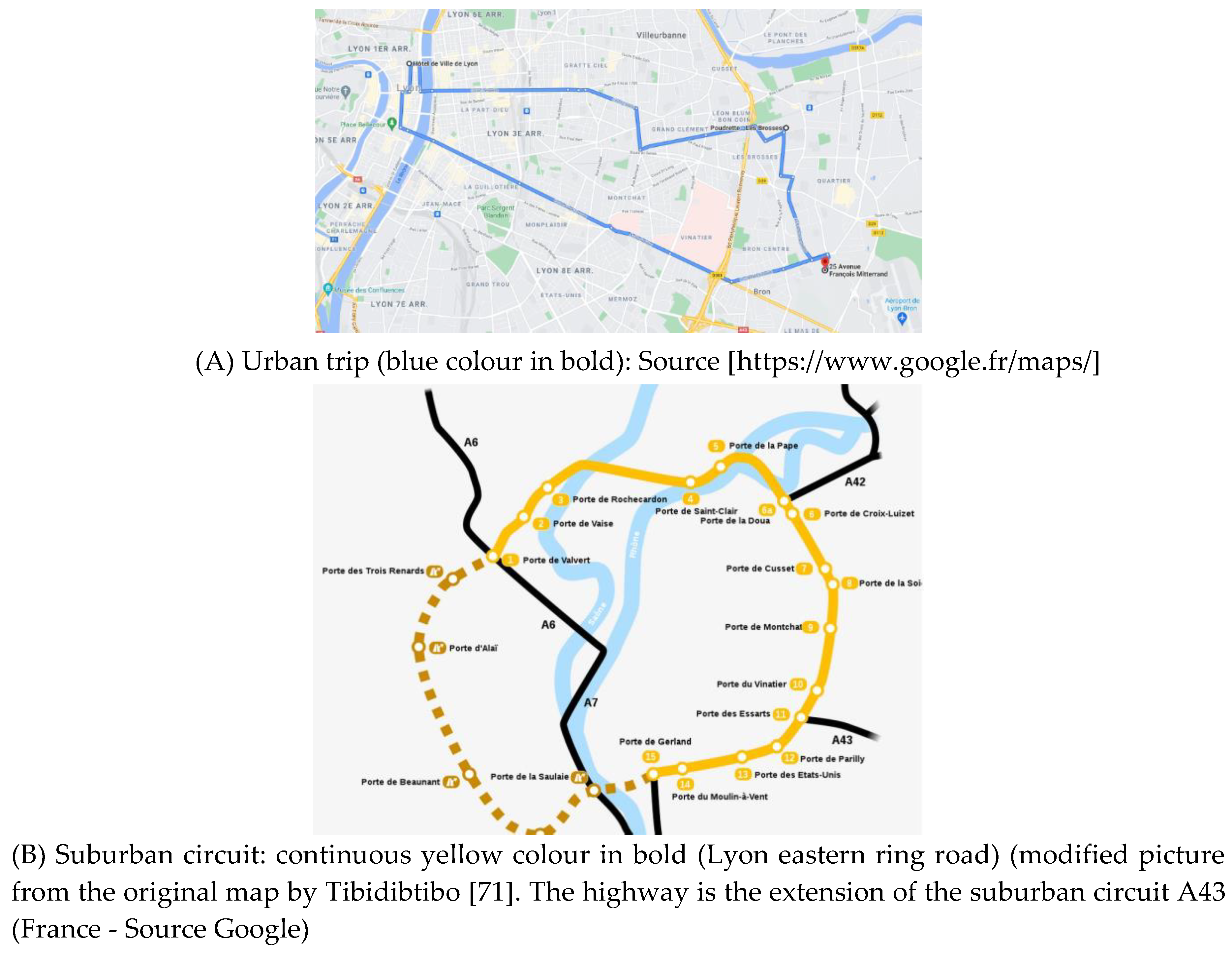
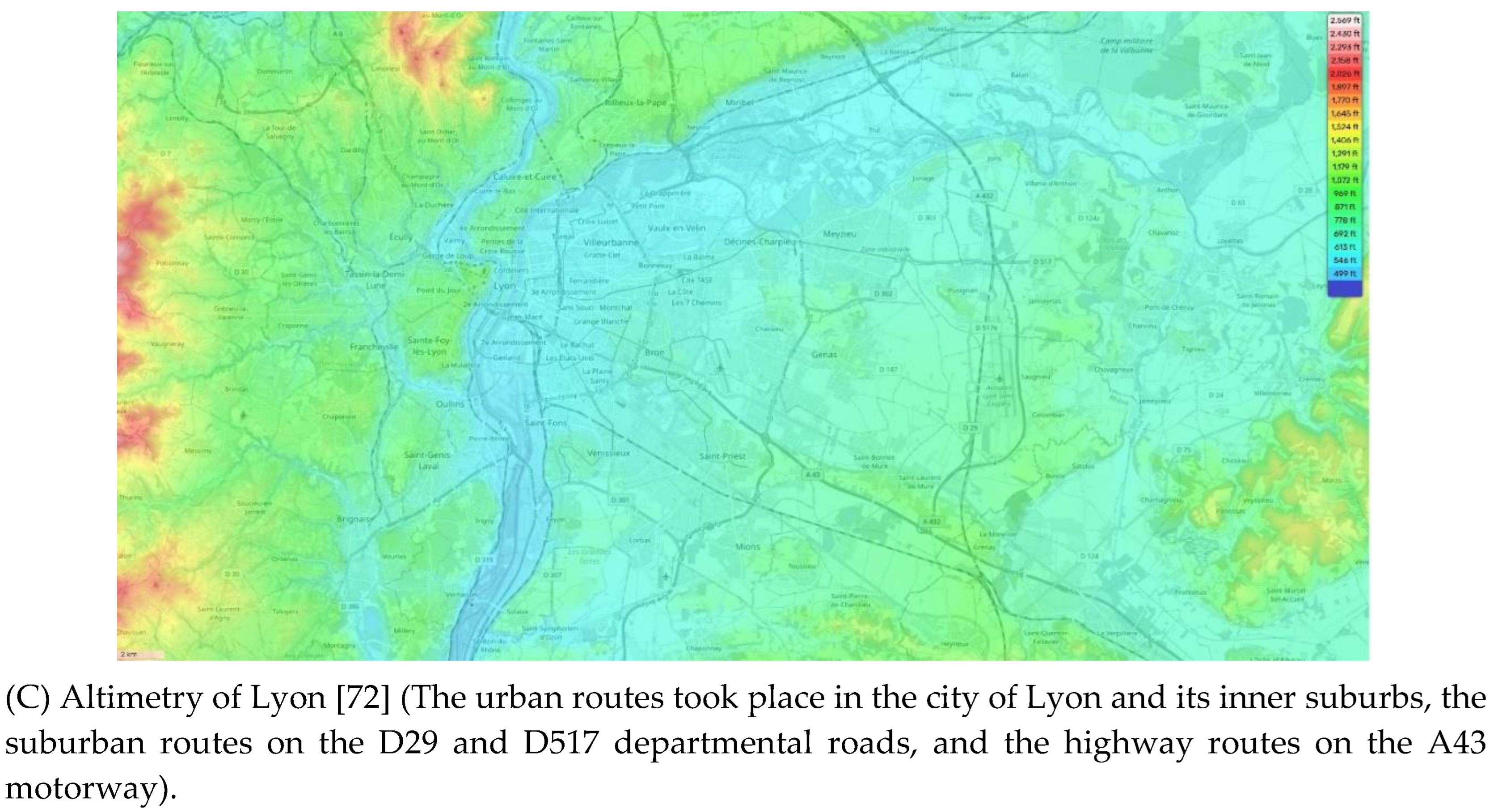
The topographical map of the city of Lyon (surface area, 47.87 km2) and its surroundings are given in the Figure 1. The average altitude of the city and surrounding area is 210m, the minimum is 161m, and the maximum is 333m (Altimetry of Lyon, 2023). The urban environment of Lyon presented an average road gradient of 12%, with the steepest gradient at 30%. In suburban and motorway environments, the average gradient was 3 % on 70% of the experimental routes, and 4.2% on the remaining 30%.

The instantaneous speed of the vehicle and position have been collected using a global positioning system under real-world monitoring with a sampling of 1 Hz. The duration of each experiment depended on the road type and the fluidity of the road traffic.

In this experimental work, the simultaneous measure of sizes of particles (granulometry) together with the collect of particles on carbon adhesive tabs (ϕ =12 and 47 mm) and on polycarbonate Whatman^® Nuclepore™ Track-Etched Membranes (ϕ = 25 mm, pore size 0.4μm) enabled the analyses of their chemical composition and identification. Membranes were considered free of traces of the chemical elements Si, Sb, S, Fe, Mg, and Na. They ensured no contamination (high chemical resistance, good thermal stability, smooth flat surface for good visibility of particles). No distinction can be made between tyres emissions and road abrasion emissions. All measuring instruments were synchronized. An electronic device, having a fixed impedance, has been used by injecting a square wave signal every 5 minutes to guarantee a synchronization between measurement systems. An optical particle counter ‘OPC’ GRIMMTM EDM 180 [73] was used to measure particles concentrations (diameter range [0.35µm,22.5µm]) with a flow rate of 1.2 l/min and 0.1μg/m³ resolution. This OPC is a real-time measurement in ambient air of PM₁₀, PM_2.5 and PM₁. It is considered as an automated monitoring system using a diagnosis software system. It has an efficient counting statistics and reproducibility of dust concentrations with low to high levels. GRIMMTM EDM 180 has been calibrated in the Grimm Group company using a dolomite dust. In comparison with other existing laboratory systems used in this research field, the preference for the GRIMM system was due to its easy operability and effectiveness (small size, light weight, high battery life, low power consumption, large data storage capacity, 12 V power supply, …). All the used data collection systems were synchronized thus allowing a good results explanation of the observed data. Before every measurement campaign, zero calibration was regulated on the GRIMM. During experimentation, a Global Positioning System (GPS) was used to collect the vehicle trajectory parameters, its speed and acceleration. Temperature of brake pads was also recorded in real-driving conditions. All measured signals were synchronized.

Each measurement was followed by blank tests lasting 15 minutes each in order to remove any impurities that may have been present in a residual way in the GRIMM pipe. Summer tyres were used to study particle emissions caused by the abrasive contact between the tyres and the road surface.

The two following sampling points were: 1. In the middle of the wheel inter-axis, 3 cm from the road surface. 2. Behind the wheel at 2 cm from the middle of the wheel and 3 cm from the road surface. The inlet sampler pipe was fixed in the vertical axis of the wheel. The particle collection tube has a diameter of ¼”. Figure 2 shows the experimental configuration of the light vehicle.

Figure 2. Two measurement points: 1. Behind the wheel (2 cm from the middle of the wheel and 3 cm from the road surface). 2. In the middle of the wheel inter-axis, 3 cm from the road surface. The particle collection tube has a diameter of ¼”.

Figure 2. Two measurement points: 1. Behind the wheel (2 cm from the middle of the wheel and 3 cm from the road surface). 2. In the middle of the wheel inter-axis, 3 cm from the road surface. The particle collection tube has a diameter of ¼”.

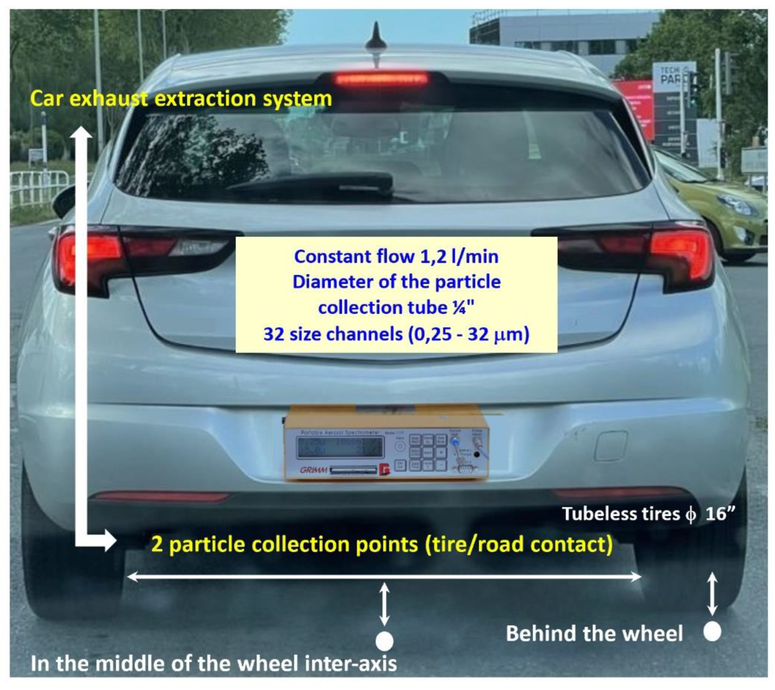
The exhaust pipe was located outside of the vehicle on the left rear side. Thus, the installed car exhaust extraction system is a 6 cm diameter tube attached to the exhaust pipe (20 cm length, followed by a 90° elbow and a 170 cm high tube). This configuration had the advantage of avoiding a mix data collection between exhaust and non-exhaust emissions. Control tests were carried out to ensure that the exhaust and non-exhaust mixture of emissions was not collected by the measurement system. Indeed, the sampling probe was placed in the centre axis between the wheels and at a 3 cm distance from the road surface. This ground distance confirmed the absence of exhaust particles in the collected data. However, measurements in this position showed that resuspension-induced particles were found. The position of the sampling, due to the screen effect of the two wheels, guaranteed that 98% of the collected particles were emitted by abrasion due to contact between the tyres and the road. The tests were carried out on days when road traffic was very low, off-peak hours, to avoid cross-contamination from other vehicles.

Brake system temperature control and exhaust emissions: the control of the brake temperature was an important element to analyse the exhaust emission rate, and subsequently the potential contamination of the collected tyre-road data. Indeed, the increase in brake friction could have had an impact in terms of contamination of measurements at the tyre-to-road contact point. This is one reason why the brakes temperature was followed during the experiments because the latter gave an information on their emission rate. A specific system to monitor these emissions was not installed but the brakes temperature was controlled in case some data seemed inconsistent. For this reason, tapered metal plates were installed on the back of the four wheels to avoid this possible contamination. The measured brake temperature is given in the following Figure 3:

Figure 3. Control of average brake temperatures during road travels.

Figure 3. Control of average brake temperatures during road travels.

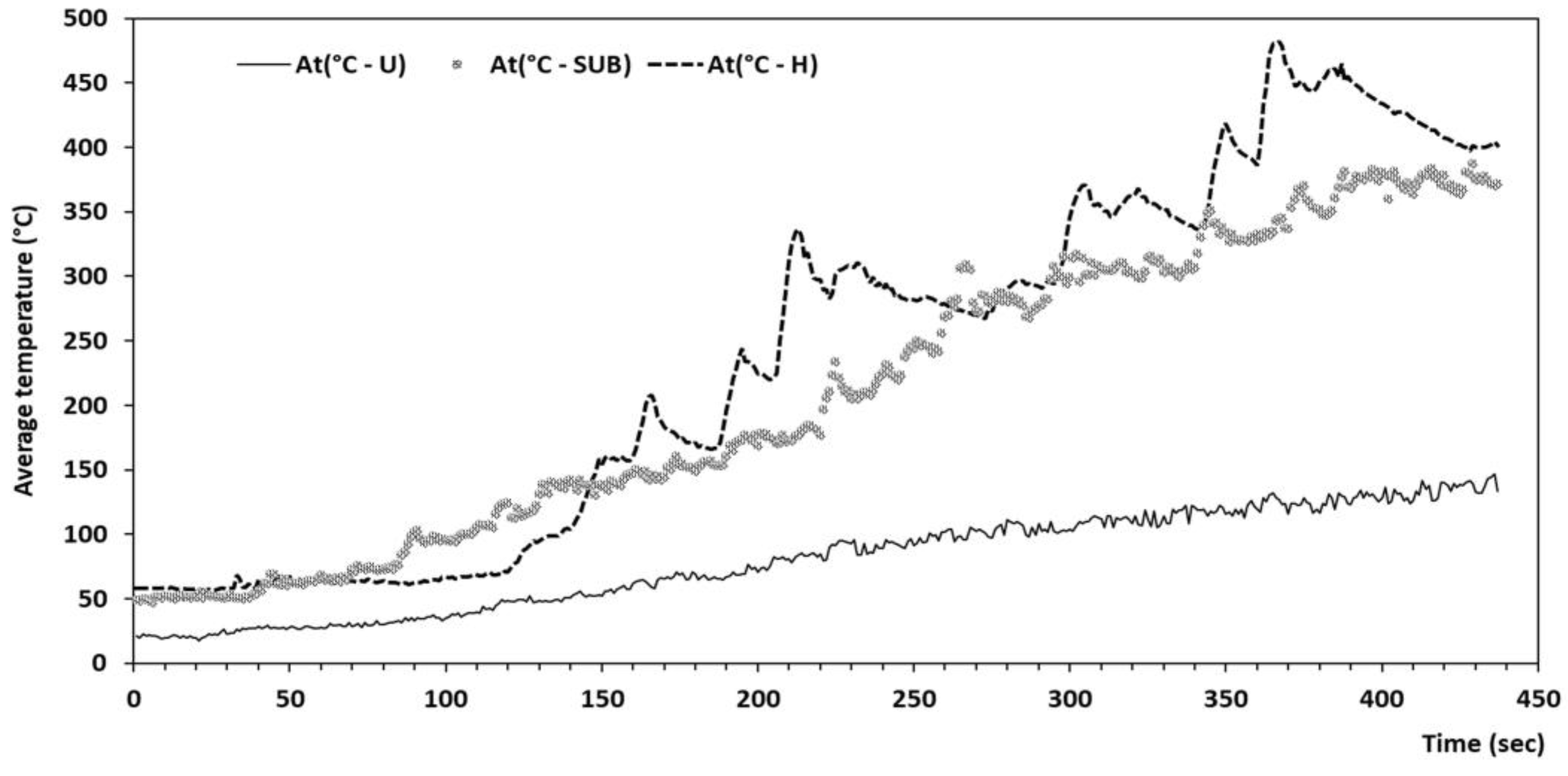
Temperature of brakes has the advance to be able to give to the research in tribology or dynamics of the contact some knowledge elements on the behaviour of the braking systems. The measured average temperatures in urban, suburban and motorway experiments are respectively 17°C, 47°C and 56°C. The maximum temperatures reached are respectively 147°c, 387°C and 482°C. The increase of the brake’s temperature occurs largely during the suburban and highway experiments (braking due to speed). With the dynamics of the vehicle in real driving conditions, no contamination of the experimental data was observed. Moreover, the results of the presented chemical analyses confirmed this. This precaution, to which was added the installation of a casing fixed on the exhaust pipeline extended up to one meter above the roof of the vehicle, enabled the avoidance of this double contamination through brake and exhaust emissions.

The aim of this paper is to calculate emission factors for pollutants emitted by tyre and road abrasion, the experiments followed the established and known procedure from the literature. Indeed, an emission factor is applied for each vehicle category in the fleet. In the case of the experiments, it was expressed as the number of pollutants per kilometer (#/km), designating the number of pollutants emitted by the vehicle over one-kilometer journey. It depended mainly on: the vehicle type, its engine and technical features (carburation: petrol, diesel, LNG, hybrid... and cubic capacity: small, medium, etc.), its date of entry into service (which determines its age and therefore its wear), average vehicle speed, track gradient, average traffic speed, and the proportion of the journey made with a cold engine.

The vehicle used was an ASTRA CDTI (year 2020) and had the following technical specifications: - Fuel type (Diesel) - Engine displacement (1496 cm³ Inline 3) - Horsepower (120 HP) - Maximum torque (221 lb-ft) - Top Speed (210 km/h).

The proportion of the experimental journey carried out with a cold engine was 2%. 84% of Lyon’s streets are limited to 30 km/h, i.e., 610 kilometres out of 727. The rest of the streets are limited to 50 km/h. Average speeds during the urban, suburban and motorway tests were 40 km/h, 80 km/h and 125 km/h respectively. Data relating to the city of Lyon (topography, slopes, and percentage of road slopes ...) are described above and have been represented in Figure 1.

2.2. Analysis of the Tyre-Road Surface Particles by SEM-EDX - Statistical Analysis

Analysis of the collected particles from dust sampling in real driving condition on the carbon membranes was carried out with the Scanning Electron Microscopy (SEM) associated with Energy Dispersive X-ray spectroscopy (EDX) [74] for identifying the elemental composition of pollutants. SEM uses an electron beam able to scan a focused stream of electrons over a given surface to produce an image with a resolution less than 1 nm. Indeed, the electrons interact with the atoms of the sample to analyse giving signals of chemical composition of the collected pollutants. The combination of these two techniques provided an identification of the pollutants elemental composition. The data generated consisted of spectra showing the chemical elements collected. Thus, energy of individual photons was measured to establish spectra representing the energy-dependent distribution of X-rays. The X-photons were captured by a solid-state detector, a lithium-doped silicon semiconductor, cooled with liquid nitrogen. X-photons cause ionization in the semiconductor. Free electron-hole pairs migrate under the effect of the polarization electric field and cause current pulses whose height is proportional to the energy of the photon. One can separate the impulses according to their height, and thus count the photons incidents according to their energy. This method has a good sensitivity in particular for photons with an energy between 0.2 and 20 keV. The number of photons is assessed and the count rate is expressed in count per second (cps). The main known limitation of this chemical analysis system is the width of each peak of the spectrum. Indeed, the enlargement of a peak could reflect the superposition of two or more chemical elements whose energy is close. The greater the enlargement of the peak, the more difficult the possibility of identifying a chemical element. For morphological analysis and the microanalysis of the collected dust, the use of the JSM-6510LV (JEOL Ltd.) was privileged as it is a high-performance SEM for a fast characterization of chemical elements. The JSM-6510LV low vacuum scanning electron microscope (SEM), with its high resolution of 3.0 nm at 30 kV, is a high-performance SEM for the reliable identification of pollutants.

The JSM was coupled to an EDX spectrometer (Oxford Aztec-DDI X MAXN 50, JEOL [75]. SEM analyses were performed at different magnifications and provided specific information on the composition of the particles. The analyses of the particles gave a comparison of their EDX spectra: retro-scattered electrons; intensity varying between 20 kV and 30kV (high resolution of 3.0 nm at 30 kV); working distance equal to 12mm (accelerating voltage from 500V to 30 kV); variation of pressure between 10 and 270 Pa; magnification x5 to 300,000 (printed as a 128mm x 96mm micrograph); objective lens apertures: three position, controllable in X⁄Y directions); maximum specimen size: 125 mm ∅ full coverage; specimen stage: eucentric goniometer (X = 80 mm, Y = 40 mm, Z = 5-48 mm, R = 360° (endless), tilt -10⁄+90°), computer controlled 2, 3 or 5 axis motor drive. The resolution is much higher compared to optical microscopes, with a greater focal depth.

The fully automated INCA software (ETAS Company) was used to analyse the collected particles. The surfaces analysed for the pollutants chemical identification were all equivalent, and were of the order of 24 mm2. INCA offered a wide variety of efficient and fast functions to analyse data (flash programming, measurement data analysis, calibration data management, and automated parameters optimization) [76]. The combined system used a motorized turntable that enabled automatic analysis of 1,000 particles for each sample. In addition to the INCA software, the application of the HCPC method for the collected data provided structure of data in terms of a partition on each granulometry interval, an identification of chemical elements, and consequently gave a hierarchy structure of the sets of different identified particles. This method was favoured over other simple classical methods that exist in literature, such as Student’s t test, …. It is based on numerical data classification methods [77,84] with a simplified application framework. Indeed, it is complete, efficient and provides excellent quality results. This method allowed the following analysis process:

-

Original data - Extraction of particle size ranges

-

Identification of intervals in order of importance

-

Assignment of intervals to identified sets of different identified particles groups

-

Homogenization of the sets according to their predominance. This step assumed, a priori, that the sets of the same identified particles were homogeneous

-

Start of the calculations and then construction of the sets of particles

-

Result with a hierarchy tree by granulometric intervals and by chemical element sets, having no consequences on relative loss of inertia of the used calculation algorithm

-

The last processing step checks error propagation and providing means, Min, gravity centres, …

Data were processed with the R software [78] which is a free and open software environment for statistical computing. It compiles and runs on a wide variety of platforms. It is a language of programming. Processing of numerical data with R [79] followed the well-numerical known steps [80–82]:

-

Import dataset in a new data matrix data

-

Build this matrix of the scaled data and apply the Ward’s minimum variance method hierarchical clustering algorithm

-

Identify and assess percentages of elements inside the same set. This step required the separation of experimental data on separate homogeneous sets of particles having equal variance that could minimize inertia in each set of data. This allowed the division of each set of data into three data sets (urban, suburban and highway), with the advantage of giving centroids of sets that measured how coherence was inside each set of identified particles

-

Choose the number of sets of identified particles that seemed relevant based on data measurements

-

Build the tree and interpret the obtained sets using the principal component analysis of FactoMineR package

-

Interpret the partition of each set versus the obtained percentages of each chemical element

-

Based on the previous steps, data analysis of results was grouped by type of route (urban – suburban – highway trips), granulometry interval and percentage of chemical elements which were identified.

Experiments in real-driving conditions were carried out by the same driver and in the same atmospheric conditions, allowing complete synthetic results without statistical bias, confirming and appreciating the quality of homogenization step previously announced. These analysis data exclude braking emissions: experiments were carried out in such a way that the particles emitted by the brakes were not recorded and did not impact whatsoever. In addition, metal wrenching and brakes abrasion were not considered. Whenever braking occurred, the corresponding data was systematically deleted. Particles were then classified in a family according to their chemical composition and the result is given in the form of a spectrum. As previously described, energy of individual photons is measured to establish spectra representing the energy-dependent distribution of X-rays.

Two concrete examples of spectra are given below (Figure 4). An elemental composition analysis was carried out using the SEM EDX to obtain an X-ray emission spectrum for the particles. They show a multitude of chemical elements identified with a net predominance of Si, Al, Ca, Mg, Fe and their components.

Figure 4. Example of two SEM-EDX spectra of particles (in Arbitrary Unit – Full scale 2054 cps).

Figure 4. Example of two SEM-EDX spectra of particles (in Arbitrary Unit – Full scale 2054 cps).

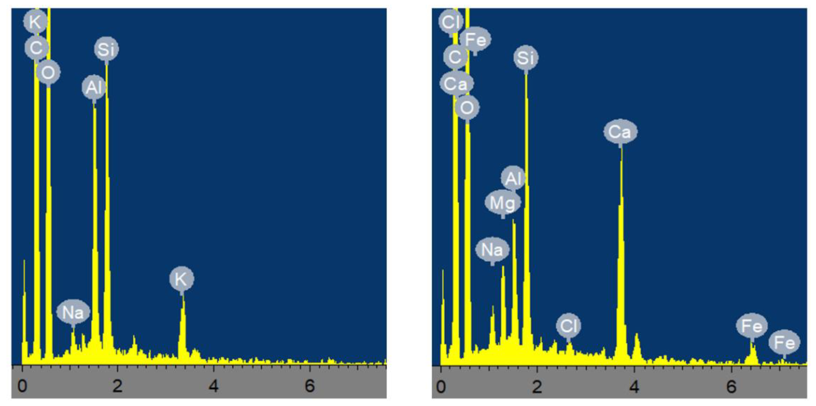
In the spectra of the particles, different peaks corresponding to C, O, Al, Si, Na, Al, Si, K, Fe, Ca, Mg, Na and Cl and traces are present. This analysis was conducted spectrum by spectrum to identify all the particles present on about a hundred sample membranes. The different set of particles obtained during this analysis were: aluminosilicate, iron and silicon compounds, iron and calcium oxides, calcium compounds, silicate without aluminum, calcium phosphate, titanium and copper compounds, chromium, sulphur and barium compounds, aluminum oxide, zirconium compound and aluminum compounds, tungsten, …, and chemical traces. Multi-elemental particles could be found in each set of compounds, with the identification of more than 33% of the total mass in the chemical element. If several elements had a mass more than 3% in the same set of particles, the heaviest element was considered and a new set of elements was created. Finally, statistical analysis of the obtained and identified particle was carried out with the statistical software R, in particular its FactoMineR package dedicated to multivariate data analysis [84].

This paper uses the identified chemical elements by the SEM-EDX. Particles emitted from the exhaust, resuspension and other contaminations, etc., were known, and systematically eliminated. In fact, this work draws on much of the open literature that has already provided information on the wide variety of pollutants considered to be contaminants in this particular case. Larger particles are deposited on a variety of substrates (buildings, infrastructures, roads, ...). Finer particles can be deposited by Brownian agitation. When there is any topography of the area in which particles are emitted, such as a street or neighbourhood, those with a mass greater than the gas molecules do not follow the air flow which is responsible for transport or dispersion phenomena. They continue moving in their original direction in which they were originally emitted. The inertia of particles allowed them to collide or stick to obstacles in the flow. The higher the flow velocity, the greater the mass of the particles. In particular, this phenomenon concerns particles with a diameter greater than 1 µm. For example, this inertia is commonly used to separate particles according to their size in cascade impactors or cyclones [2,6,8]. Inertia of chemical species has been used to analyse the homogeneity of the flow. Chemical species ‘i’ were assessed in all the measured samples. Calculating the v_test meant applying the following formula [84] for species ‘i’ (i ∈ groups) to verify the homogeneity degree of flow of particles. These sets consist of chemical elements with the same properties or the same chemical identification obtained by a count:

$$v\_test[i]=\sqrt{N_{[{\cup }_I]}}\times \frac{f_{i/\left[I\right]}-f_{[\cup I]}}{\sqrt{\frac{N_{i/\left[I\right]}-N_{\left[{\cup }_I\right]}}{N_{i/\left[I\right]}-1}\times f_{[\cup I]}\times (1-f_{[\cup I]})}}$$

where:

- i: chemical specie (pollutant)

$f_{i/\left[I\right]}$: frequency of the ‘i’ specie in the set I

$f_{[\cup I]}$: frequency of the ‘i’ specie in the all sets of data

$N_{i/\left[I\right]}$: the relative number of ‘i’ specie in the set I versus the size

$N_{\left[{\cup }_I\right]}$: the relative number of ‘i’ specie in all the sets of data I versus the total size of the sets

I is the set of identical chemical species, identified by SEM-EDX, analysed for a given surface of the sampling membrane. This surface may correspond to the total surface of the membrane if the analysis is performed on a single membrane. In this particular case, the MEB analysis surface was defined for all the particle collection membranes

v_test is well-known to be sensitive to the identification sensitivity analysis. It is used in this paper to categorial variables “i” in terms of chemical identification. This is a necessary and sufficient condition when sets of species are different.

3. Results

Individual particle analyses SEM-EDX and global analysis (granulometry - particle size) were performed, as well as the calculation of the overall values for the data obtained at the SEM-EDX, this in order to make comparisons. Thus, Figure 5 presents the variations of the mean values of the particle number according to the analysis by the SEM-EDX of the collected particles on the membranes, and by the particle size analyser (PSA) vs. the vehicle speed. This analysis was conducted for the three types of trips: 6 urban trips, 2 sub-urban trips and 3 highway trips. The respective speed values for the three routes in France (45 km/h, 90 km/h and 130 km/h) represent the maximum values to be performed per site.

Figure 5. Number of particles depending on the type of analysis (PSA and SEM-EDX) and road (urban, suburban and motorway respectively with speed limit of 45 km/h, 90 km/h, 130 km/h).

Figure 5. Number of particles depending on the type of analysis (PSA and SEM-EDX) and road (urban, suburban and motorway respectively with speed limit of 45 km/h, 90 km/h, 130 km/h).

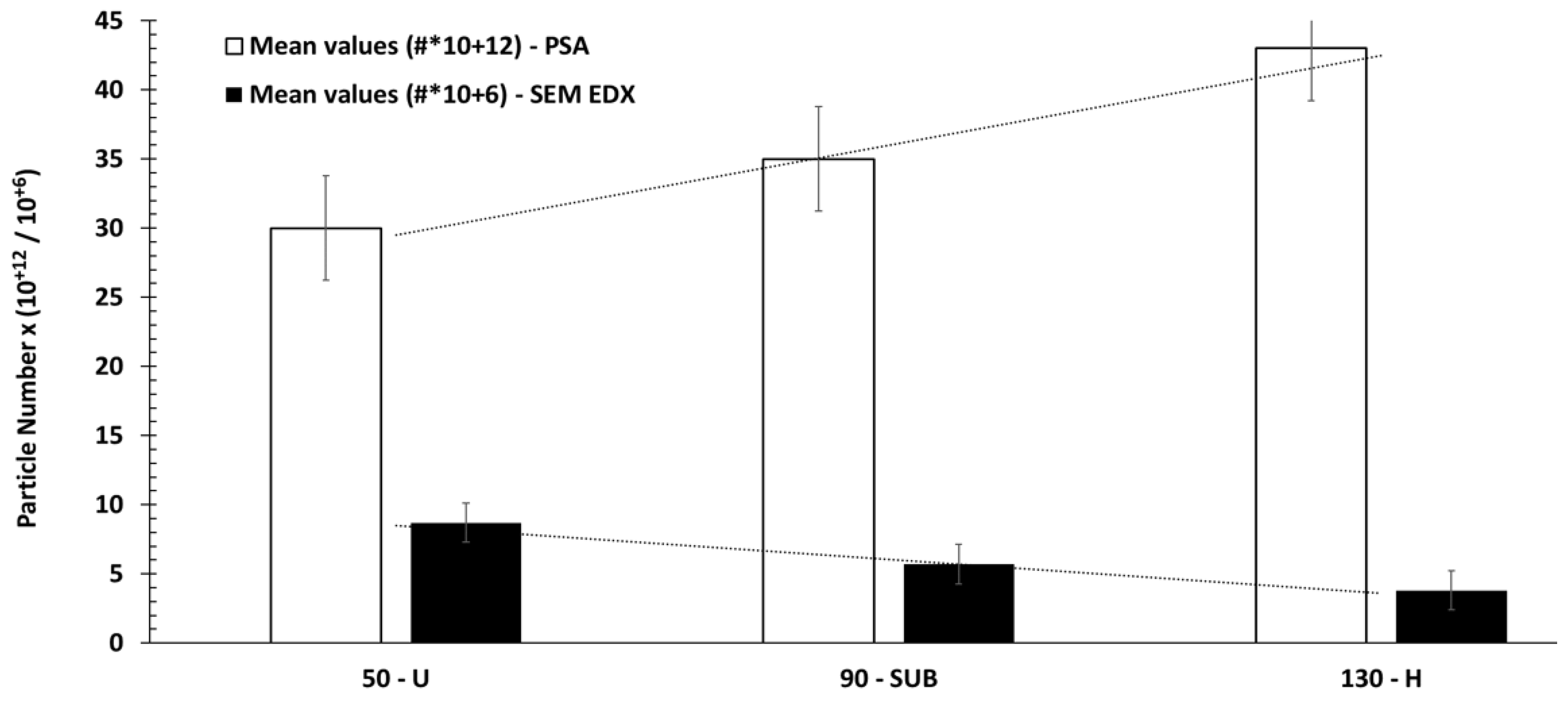
First of all, we can see that there is an effect of the vehicle speed. The number of particles emitted increases with the speed when measurements are made with a particle size analyser. A slight inverse effect occurred when analysis was performed with the SEM-EDX. This behaviour in the number evolution is normal and is due to the fact that a chosen surface was targeted for EDX SEM analysis. The measured average particle number values are:

-

Particle size analyser: (30, 35, 43) 10⁺¹² particles.

-

SEM-EDX: (8.7, 5.7, 3.8) 10⁺⁶ particles.

The ratios (particle size count/ SEM-EDX count) are respectively of 6.4 10⁺⁶, 6.2 10⁺⁶ and 11.3 10⁺⁶ for urban, suburban and highway trips.

The following analysis will make it possible to extrapolate this number of particles for the surrounding particles collected throughout the membrane.

Several observations can be noted:

• A high factor of more that 10⁺⁶ is found between the particle size values and the assessment of the total number of particles from the SEM-EDX results. This seems natural because the collection on the membranes is purely qualitative and serves more for chemical identification.
• Despite uncertainties in both particle size count, there is an inversion of the curves between particle size and chemical particle counting as a function of velocity. On the one hand, considering SEM-EDX counting, more particles were collected in the urban area than on highways because of the vehicle speed. This is certainly due to the dynamics of emissions as a function. On the other hand, the inversion of this curve, obtained by the particles collected by granulometry method, seems in favour of the speed. The faster we drive, the more we collect. This Figure confirms that the physico-chemistry is preserved with this double collection independently of the variations that can be observed. Therefore, precaution must be taken when counting particles from the collection on membranes for chemical analyses. In this case, the emission dynamics, which is a function of the speed of the vehicle, could not be confirmed.

In conclusion, counting from the SEM-EDX is a qualitative count in favour of the chemical identification of emitted particles. On the other hand, particle size counting is quantitative. Based on the collection of particle size data, the analysis of the most emissive particle size intervals is shown in the following Table 2 in order of importance in terms of emission:

Table 2. Predominance order of the collected particle sizes (U, SUB, H).

Predominance order of particle sizes	U	SUB	H
1st class	<1µm	<1µm	<1µm
2nd class	1-2µm	1-2µm	1-2µm
3rd class	-	2-3µm	2-3µm
4th class	-	-	3-4µm

Table 2. Predominance order of the collected particle sizes (U, SUB, H).

Predominance order of particle sizes	U	SUB	H
1st class	<1µm	<1µm	<1µm
2nd class	1-2µm	1-2µm	1-2µm
3rd class	-	2-3µm	2-3µm
4th class	-	-	3-4µm

We can observe in this table that the grain size range widens from the urban to the motorway emissions. The particles less than 1 µm are the most present in the three road routes; followed by interval [1 µm, 2 µm], and finally [2 µm, 3 µm] for the sub and [3 µm, 4 µm] for highway. The synthesis thus provides a general predominance of particles emitted in the particle size range respectively [<1 µm, 2 µm], [<1 µm, 3 µm] and [<1 µm, 4 µm] for urban, suburban and highway experiments.

The percentages of the predominant particle size classes are 72.7% for the first two combined classes, 21% for the third and 6.3% for the fourth. The effect of the speed of the vehicle, and therefore the potential for collecting particles online, is certainly obvious. These percentages are therefore consistent with what was observed in the literature [6,17,27,85–87]. The first two particle size classes are known to have the highest degree of toxicity [88] because they easily penetrate the lungs and cross biological barriers to be located in vital organs, may cause significant health consequences.

Number concentrations are therefore dominated by particles <1μm, while most of the mass was in particles >1μm. This result agrees with the work of Alves et al. [89]. These authors had found rather 0.5μm instead of 1μm, which is not really in contradiction with this result if it is refined further, thus it would not be necessary because it does not improve the results.

Particle larger sizes were not collected because they were deposited on the road surface. This finding completes the obtained results by Iijima et al. [90] in terms of size distribution (1–10μm and 2–3μm). The results indicated in this article confirm the analysis made by Liu et al. 54] who identified the variations in particle size range, in particular in 0,25-4μm interval. In addition, Harrison et al. [41] confirmed in their analysis of the non-exhaust emissions, i.e., from the brakes abrasion, tyres and wear of the road surface, as well as from resuspension of road dusts, that the emitted particles have to be in both the coarse (PM_2.5-10) and fine (PM_2.5) fractions, with a larger proportion in the former. The results of the experiments agree with those obtained in the open literature, in particular with Beji et al. [12], Harrison et al. [41], Liu et al. [54], Piscitello et al. [86] and Zhang et al. [87,91].

Concerning the chemical analysis, data processing shows a wide variety of chemical elements emitted in real driving situations. During chemical analysis, the systematic presence of carbon and oxygen was noticed in all analysed tabs (membranes). This is found in almost all SEM-EDX analyses reported in the open literature [6,27,40].

In order to identify the tyres-road surface particles, carbon and oxygen C and O were excluded from the statistical analysis. In this paper, neither the production modes of particles nor their shapes were analysed because this would require a very complex additional experimental work. Individual analysis is very expensive in terms of computational time. These modes and shapes that could be subject to further works are: 1. Nucleation mode (particles having a spherical shape with ϕ < 30 nm). 2. Accumulation (particles having an angular morphology with 100 nm < ϕ < 200 nm). 3. Coarse mode (particles aggregated with 1 µm < ϕ).

Analysing the particle number collected by analyser allowed to calculate the emission factor for four different situations: 1. on an urban site where the traffic speed is between 30 and 50 km/h; 2. on a suburban site where the speed limit is 90 km/h; 3. on a highway where the speed limit is 130 km/h; 4. in a traffic zone on an urban site in the city of Lyon (France). Granulometric data was collected with ATMO AURA fixed systems. Among the data collected, the following selection was made: 6 urban routes (U1 to U6), 2 suburbans (SUB1 and SUB2) and three highways (H1 to H3). For comparison, the collection then analyses focus on a series of data recorded during 4 different days corresponding to a static urban traffic site (S1 toS4). The data were collected during days when the weather conditions were identical to the whole other experiments (U, SUB, H).

Figure 6 below shows emission factors EF in number of particles per km travelled (#/km).

Figure 6. Emission factors for three different driving situations. Maximum authorized speed [Urban ‘U’ (50 km/h) – Suburban ‘SUB’ (90 km/h) – Highway ‘H’ (130 km/h)].

Figure 6. Emission factors for three different driving situations. Maximum authorized speed [Urban ‘U’ (50 km/h) – Suburban ‘SUB’ (90 km/h) – Highway ‘H’ (130 km/h)].

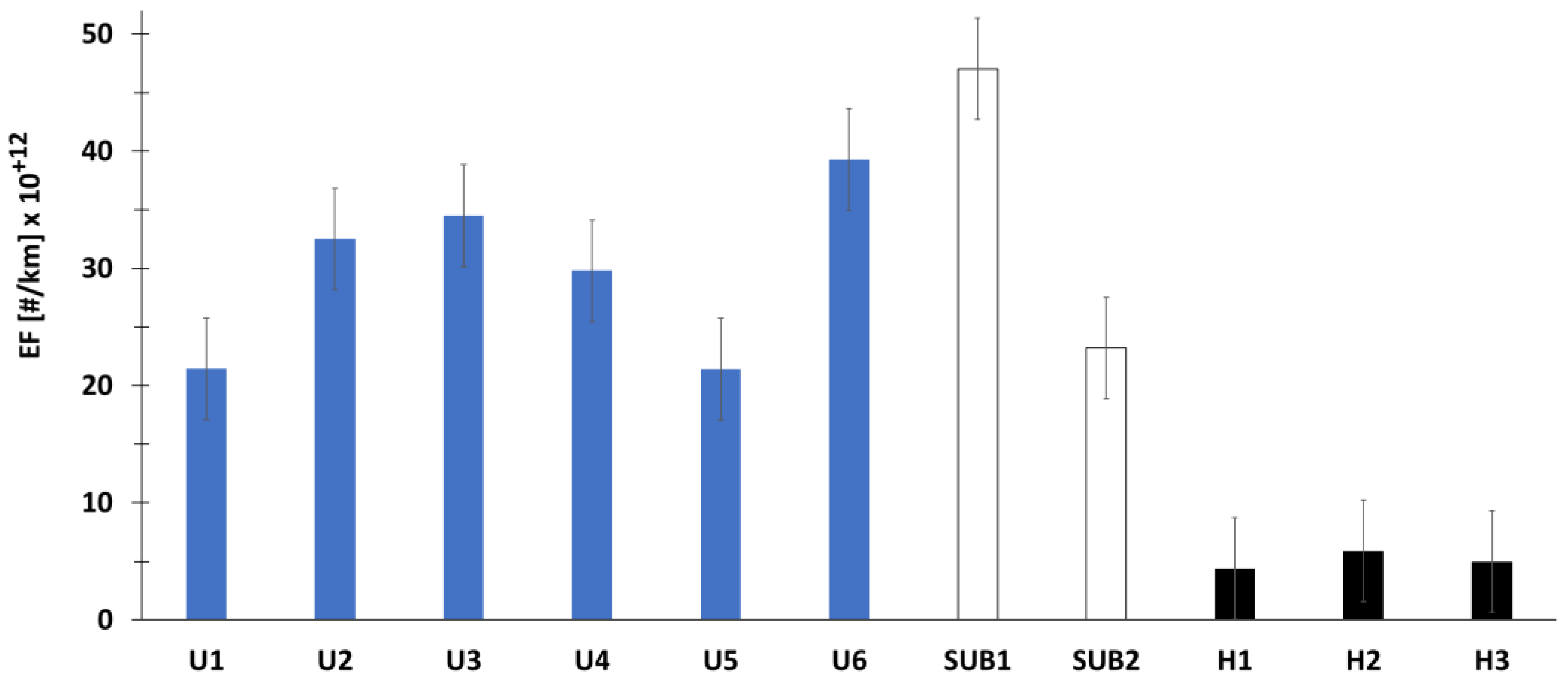
The emission factors are of the order of 30 10⁺¹² #/km and 35 10⁺¹² #/km for urban and sub-urban respectively. We observe that there is a difference between urban and peri-urban of 5 10⁺¹² #/km. However, on highway, the emission factor, on average in the order of 5 10⁺¹² #/km, is much lower than the two previous situations. Emission factor obtained on the highway trip is of the same order of the magnitude as the difference between urban routes and suburban driving situations. The number of particles was calculated for a duration equal to the duration of urban experiments U1 to U6. Finally, for the urban traffic situation site, we have on average a number equal to 43 10⁺¹² #/cm³ (S). This value (number of particles per unit volume) cannot be related to an emission factor obtained in real driving conditions. However, this higher value, in static urban site, can be considered quite high. This is due to the accumulation of pollutants in a fixed urban site, corresponding to the ambient air pollution in this urban point location.

The obtained EF for the three types of experiments are above the value of the euro 6 standard (fixed at 6 10⁺¹¹ #/km) for both diesel and petrol vehicles. It can also be noted that these EFs are below of the values corresponding to diesel vehicles not equipped with particle filter (6 10⁺¹³ #/km) where ratios are of 2 (U), 1.7 (SUB), 12 (H) and 1.4 (S). As a reminder, the New European Driving Cycle gave a limit value of 6 10⁺¹¹ #/km (Euro 6b) for PN (number of particles per km) for spark-ignition engines (gasoline, LPG, etc.), including hybrids, and a limit value of 6 10⁺¹² #/km for diesel engines only, including hybrids. In the future, we shall be seeing stricter regulations on the limit values that must not be exceeded.

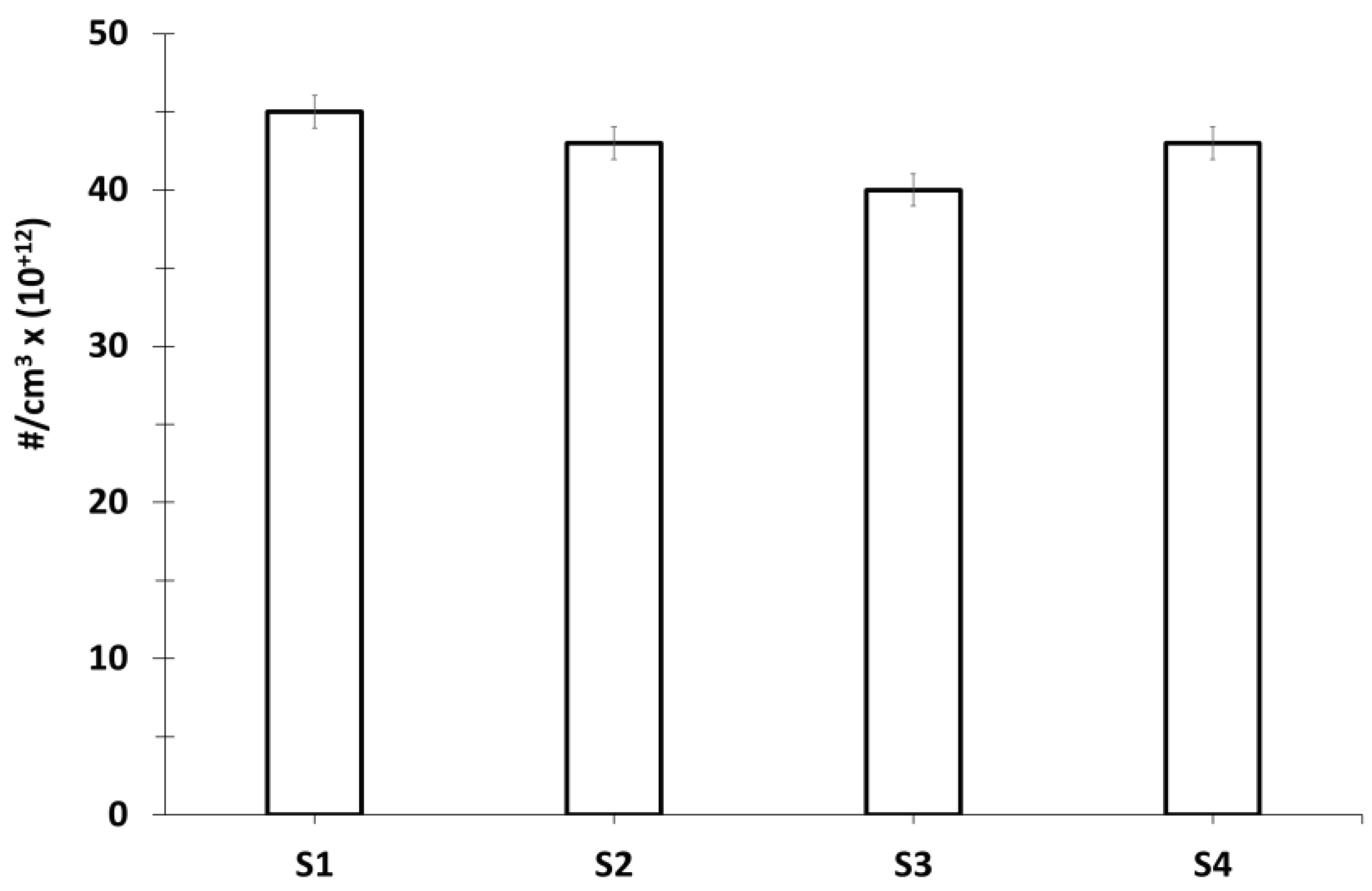
It can be noted that the number of particles is quite similar in the city static situation compared to experiments performed in real driving conditions. This is due both to the dispersion of pollutants but also to the effect of accumulation in a localized static point. Figure 7 shows the number of particles per cm³ at this static point in the urban area of Lyon. For all the performed experimental measurements, with uncertainties, the number of particles per cm³ is greater in static situation in city (≈ 42.8 10⁺¹² #/cm³) than in real driving situation (approximately 30 10⁺¹² #/cm³ in urban and 35,1 10⁺¹² #/cm³ in suburban). This is due both to the dispersion of pollutants but also to the effect of accumulation in a localized unpoint.

Figure 7. Evaluation of the average number of particles per cm³ in the traffic site, at a fixed location in an urban environment (S1 – S2 – S3 – S4).

Figure 7. Evaluation of the average number of particles per cm³ in the traffic site, at a fixed location in an urban environment (S1 – S2 – S3 – S4).

These results allowed to evaluate the average corrective factor ACF between analysis of emission factors obtained by particle size analysis and those obtained by identification using the MED EDX. These average factors are respectively 3,4 10⁺⁶ (urban), 6,1 10⁺⁶ (suburban) and 11,3 10⁺⁶ (highway).

Thus, the number of particles used in the chemical identification of pollutants, obtained by the SEM-EDX analysis, is multiplied by this corrective factor to obtain the number of particles that would be analysed online in real driving situation. This analysis enabled to establish the emission factors by chemical element, as presented in the Figure 8 which shows the average emission factors EF for the 19 identified pollutants.

Figure 8. Emission Factors for the identified individual pollutants in real driving.

Figure 8. Emission Factors for the identified individual pollutants in real driving.

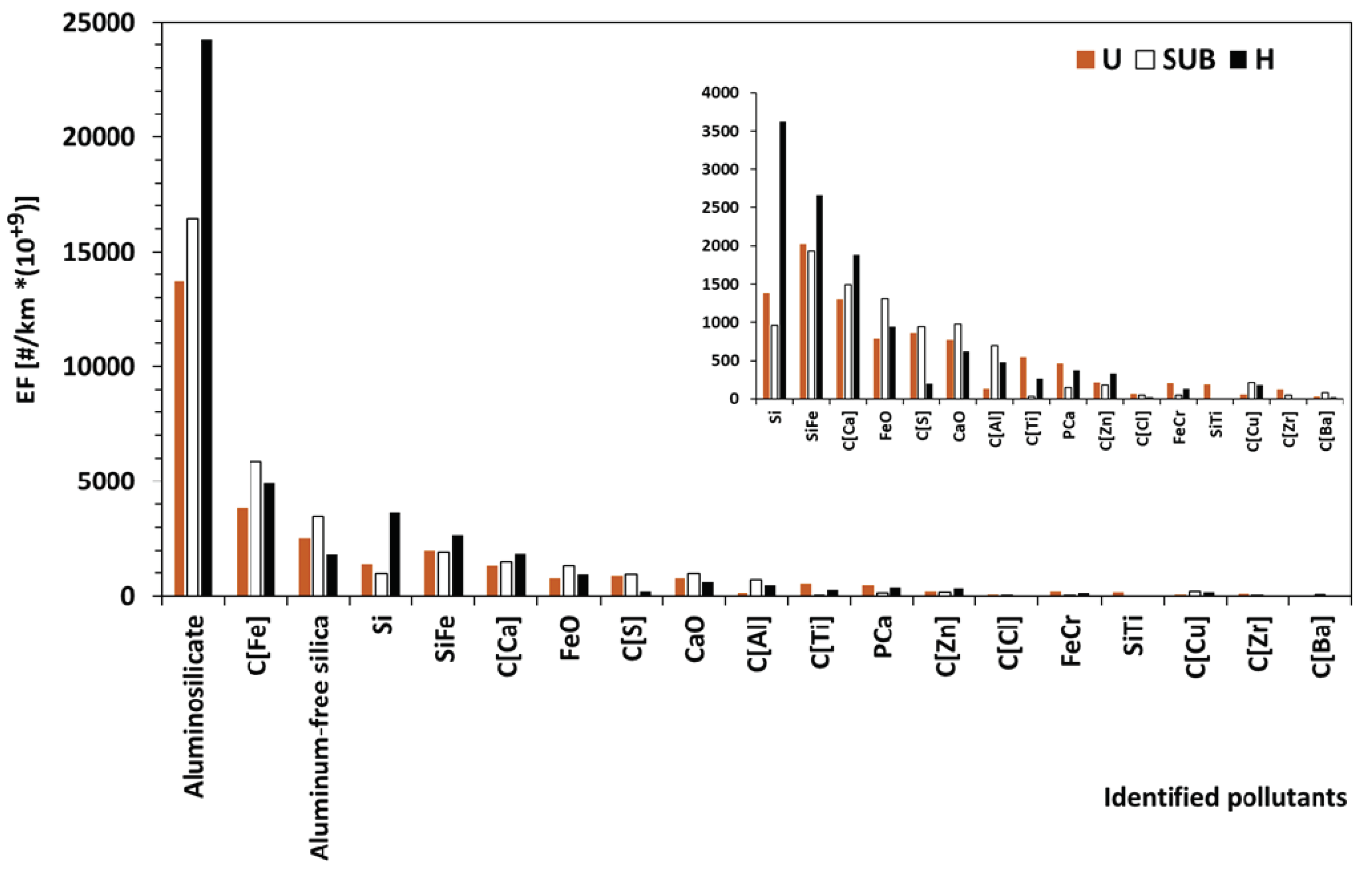
We note the predominance of aluminosilicate, Fe components, aluminum free of silica, Si, SIFe, Ca components, and FeO. For the rest of the pollutants, the A_EFs are low. This does not mean that they should not be taken-into-account in any environmental or health impact analysis, as this will naturally depend on the volume of the vehicle fleet.

Table 3 gives the emission factors for 19 pollutants identified using the SEM EDX technique. These are emission factors obtained experimentally in the region closest to their emission sources (tyres - road surface). Analysis of pollutants taken individually, EF ranges from 0.003 to 18.142 10⁺¹² #/km.

Table 3. Emission factor for 19 individual pollutants.

Identified pollutants by SEM-EDX		Emission Factor [#/km *10+9]	Percentages (compared to the total number)
1	Aluminosilicate	18142±597	50,9%
2	C[Fe]	4881±175	13,7%
3	Aluminum -free silica	2612±57	7,3%
4	SiFe	2206±60	6,2%
5	Si	1989±36	5,6%
6	C[Ca]	1558±32	4,4%
7	FeO	1013±33	2,8%
8	CaO	789±26	2,2%
9	C[S]	667±25	1,9%
10	C[Al]	436±27	1,2%
11	PCa	329±17	0,9%
12	C[Ti]	281±11	0,8%
13	C[Zn]	240±8	0,7%
14	C[Cu]	152±5	0,4%
15	FeCr	129±9	0,4%
16	SiTi	64±7	0,2%
17	C[Zr]	58±9	0,2%
18	C[Ba]	46±11	0,1%
19	C[Cl]	39±11	0,1%

Table 3. Emission factor for 19 individual pollutants.

Identified pollutants by SEM-EDX		Emission Factor [#/km *10+9]	Percentages (compared to the total number)
1	Aluminosilicate	18142±597	50,9%
2	C[Fe]	4881±175	13,7%
3	Aluminum -free silica	2612±57	7,3%
4	SiFe	2206±60	6,2%
5	Si	1989±36	5,6%
6	C[Ca]	1558±32	4,4%
7	FeO	1013±33	2,8%
8	CaO	789±26	2,2%
9	C[S]	667±25	1,9%
10	C[Al]	436±27	1,2%
11	PCa	329±17	0,9%
12	C[Ti]	281±11	0,8%
13	C[Zn]	240±8	0,7%
14	C[Cu]	152±5	0,4%
15	FeCr	129±9	0,4%
16	SiTi	64±7	0,2%
17	C[Zr]	58±9	0,2%
18	C[Ba]	46±11	0,1%
19	C[Cl]	39±11	0,1%

By way of comparison, the euro 6 standard is set at 6 10⁺¹¹ #/km for both diesel and gasoline. For diesel vehicles not fitted with a filter, the given value is 6 10⁺¹³.

Experiments do not take into-account a heterogeneous mixture of components from (P, Cl, Fe, Ba, Cr, Zr) which represents a percentage of less than 0.1% of the total number of particles identified.

Pearson and Spearman correlations [92] applied to the data according to the different variables (urban, suburban and highway routes, the same vehicle equipped with the same tyres, the weight of the vehicle, nature of the road, …), showed that correlations were significant (with p< 0.02).

In addition, analysis of the inertia of chemical species ‘i’ has been carried out to confirm the homogeneity of their identification. Assessment of v_test was also done especially for the comparison between identified pollutants and their numbers. Characterization of each pollutant and the significance test was calculated:

v_test is equal to 1.92 for urban sets of data of pollutants, 1.97 for suburban, and -1.87 for highway (p ≌ 5%). The inertia of chemical species, in the three trips, is definitively homogeneous, and analysis is therefore considered significant (v_test ≌ ±2).

It should be remembered that this finding completes and provides additional information to the work by Dahl et al. [37], Panko et al. [85], Piscitello et al. [86], Iijima et al. [90], Zhang et al. [92] and Kaul and Sharma [93]. Piscitello et al. [86] had confirmed that the emission rate of the non-exhaust pollutants reached 90% by mass of total traffic-related PM emitted. They gave emission factors as follows: 0.3 mg/km to 7.4 mg/km for tire wear; resuspended dust: 5.4 mg/km to 330 mg/km.

Finally, an attempt was made to approximate the EF of the PM₁₀ and PM_2.5 from the calculations by Zhang et al. [91]. Indeed, by assessing the density of those two major air pollution determinants, with a conversion of the number into mass and assuming that all the particles are identical and spherical, the obtained FE is of 1.45 mg/km for PM₁₀ and 0.35 mg/km for PM_2.5. These FE values are close to those obtained by Zhang et al. [91] (0.21 mg/km for PM_2.5 and 1.27 mg/km for PM₁₀), who carried out experiments on a tyre dynamometer. The small difference can be attributed to the fact that this new additional work assesses all the emissions from the tyre-road surface wear and not the emissions from the tyre alone.

This shows that the new methodological approach used in this paper is particularly effective in assessing pollutant emission factors. It is a new alternative to existing methods that are sometimes very difficult and costly to implement. In addition, Alves et al. [89] had generated wear particles on a road simulator to study the interactions between tyres and a composite road surface. They found that the emission factor due to wear between their particular road surface and the tyres was of the order of 2 mg/km. On the one hand, work carried out on any simulator under controlled conditions often deviates from reality or from actual vehicle use. On the other hand, this estimate is not very far removed from the new results being produced and obtained with experiments carried out in real driving situations.

4. Conclusions

This paper presents an original experimental approach combining collection of particles emissions induced by the tyres-road surface wear in real driving conditions, in urban, suburban and highway routes. Comparatively, the data was collected on a site located in the city, on a boulevard where traffic is very important. To determine the chemical compositions and then emission factors of particles emitted by tyre-road surface wear without contamination from brake dust, measurements were performed in real driving conditions. The SEM-EDX has been used to identify the measured chemical elements and their nature. Predominant particles emitted by tyres-road surface have been analysed and emission factors for 19 identified pollutants assessed for the first time using this new approach. The major findings of this study can be summarized as follows:

1. The mainly most measured tyres-road surface particles were smaller than 1 µm for the three road routes; followed by interval size particles [1 µm, 2 µm]. Then, in the third position we have the size range [2 µm, 3 µm] for suburban and highway; and in the fourth position the range [3 µm, 4 µm] for highway alone. It should be noted that particles of sizes between 2 and 4 µm are emitted in urban, between 3 to 4 µm in suburban experiments but at low proportions due to emissions dynamics (vehicle-tire-pavement) related to the movement of the vehicle and the tribology of the materials that constitute the tyres and the road surface.

2. Data processing showed a wide variety of chemical elements emitted in real driving situations. The systematic presence of carbon and oxygen was noticed.

3. Emission factors EF were calculated on the basis of granulometric and global chemical analysis of the measured date: average values for all measured pollutants are 30 10⁺¹² #/km and 35 10⁺¹² #/km respectively for urban and sub-urban. However, on highway, EF is equal to 5 10⁺¹² #/km, about 6 to 7 times lower than the previous two. Analysis for pollutants taken individually, the EF ranges from 0.003 to 18.142 10⁺¹²#/km. Significance test analysis was carried-out for the identified pollutant and their EF. v_test is found to be varied between 1.87 and 1.97 (p ≌ 5%). The inertia of chemical pollutants is definitively homogeneous, and analysis is therefore considered significant because the v_test is ≌ ±2.

4. The obtained EF are above the value of the euro 6 standard of 6 10+11 #/km for both diesel and petrol vehicles. EFs are below the values corresponding to diesel vehicles not equipped with particulate filter (6 10+13#/km). As a reminder, the New European Driving Cycle gave a limit value of 6 10⁺¹¹#/km (Euro 6b) for PN (number of particles per km) for spark-ignition engines (gasoline, LPG, etc.), including hybrids, and a limit value of 6 10⁺¹² #/km for diesel engines only, including hybrids.

5. Assessment of EF of the PM₁₀ and PM_2.5 emitted by the tyre-road surface wear are 1.45 mg/km and 0.35 mg/km, respectively.

6. The number of particles number per volume element in static situation in the city is ≈ 42.8 10⁺¹² #/cm³. This number of particles is stable almost every day except for summer holiday periods and Sundays when urban traffic is low in the city. In real driving situation, we obtained 30 10⁺¹² #/cm³ in urban and 35 10⁺¹² #/cm³ in suburban. The larger measured number on the fixed site is due both to the dispersion of pollutants and also to the effect of accumulation in a localized unpoint.

These results show that the methodological approach, used in this paper, is particularly effective in assessing pollutant emission factors. This kind of approach is a new alternative to existing methods. The significant obtained results in this paper thus provide reliable information to help improve emission models, making them more accurate and applicable. Further research, integrating the phenomena of resuspension of particles in the air, is necessary. These researchers will bring other scientific knowledge to the work presented in this paper. They will have to consider the nature of the materials of the road surfaces and tyres. Their physico-chemical characteristics must therefore be specified. Thus, a metrological and methodological development must be carried-out to separate the sources of particles emitted by the tyres, the road surface and the resuspension. These particles will have to be analysed individually, and if possible online to avoid chemical transformations that induce secondary pollution because airborne particles can differ significantly from friction materials. Then, experimental conditions will have to be controlled, and if necessary supported by new tool developments. The problem could become insoluble if we were not to take into-account the “complex” mixing effect between exhaust and non-exhaust emissions.

The results presented in this paper will contribute to future regulations for road vehicles (thermal, hybrid, electric, autonomous). Further scientific work, i.e., analysing exposure-impact relationships to particles emitted by abrasion of tyres and road surface, is needed to complete the development of technical and legislative recommendations, as well as health guidelines. Appropriate regulations will provide the framework for public and environmental policies. They will also provide the necessary support for emerging technologies which objectives are the well-being of population and improvement of the environment.

References

- Casati, R.; Scheer, V.; Vogt, R.; Benter, T. Measurement of nucleation and soot mode particle emission from a diesel passenger car in real world and laboratory in situ dilution. Atmos. Environ. 2007, 41, 2125–2135. [Google Scholar] [CrossRef]
- Belkacem, I.; Khardi, S.; Helali, A.; Slimi, K.; Serindat, S. The influence of urban road traffic on nanoparticles: Roadside measurements. Atmos. Environ. 2020, 242, 117786. [Google Scholar] [CrossRef]
- Schneider, I.L.; Teixeira, E.C.; Dotto, G.L.; Yang, C.X.; Silva, L.F. Geochemical study of submicron particulate matter (PM1) in a metropolitan area. GSF 2020, 101130. [Google Scholar] [CrossRef]
- Zhu, Y.; Hinds, W.C. Predicting particle number concentrations near a highway based on vertical concentration profile. Atmos. Environ. 2005, 39, 1557–1566. [Google Scholar] [CrossRef]
- Giechaskiel, B.; Riccobono, F.; Vlachos, T.; Mendoza-Villafuerte, P.; Suarez-Bertoa, R.; Fontaras, G.; Bonnel, P.; Weiss, M. Vehicle Emission Factors of Solid Nanoparticles in the Laboratory and on the Road Using Portable Emission Measurement Systems (PEMS). Front. Environ. Sci. 2015, 3, 82. [Google Scholar] [CrossRef]
- Khardi, S.; Deboudt, K.; Muresan, B.; Beji, A.; Tassel, P.; Serindat, S.; Perret, P.; Cerezo, V.; Louis, S.; Lumière, L.; et al. Projet CAPTATUS « Caractérisation physico-chimiques des particules émises hors échappement par les véhicules routiers ». N° de contrat: 15.66.C0016. Rapport final. October 2018.
- Kajino, M.; Kayaba, S.; Ishihara, Y.; Iwamoto, Y.; Okuda, T.; Okochi, H. Numerical simulation of IL-8-based relative inflammation potentials of aerosol particles from vehicle exhaust and non-exhaust emission sources in Japan. Atmos. Environ. X 2024, 21, 100237. [Google Scholar] [CrossRef]
- Belkacem, I.; Helali, A.; Khardi, S.; Chrouda, A.; Slimi, K. Road traffic nanoparticles characteristics: sustainable environment and mobility. Geoscience Frontiers GSF 2022, 13, 101196. [Google Scholar] [CrossRef]
- Trejos, E.M.; Silva, L.F.; Hower, J.C.; Flores, E.M.; González, C.M.; Pachón, J.E.; Aristizábal, B.H. Volcanic emissions and atmospheric pollution: A study of nanoparticles. GSF 2021, 12, 746–755. [Google Scholar] [CrossRef]
- Silva, L.F.; Schneider, I.L.; Artaxo, P.; Núñez-Blanco, Y.; Pinto, D.; Flores, É.M.; Gómez-Plata. L.; Ramirez, O.; Dotto, G.L. Particulate matter geochemistry of a highly industrialized region in the Caribbean: Basis for future toxicological studies. GSF 2020, 13, 101115. [Google Scholar]
- Beji, A.; Deboudt, K.; Khardi, S.; Muresan, B.; Lumiere, L. Determinants of rear-of-wheel and tire-road wear particle emissions by light-duty vehicles using on-road and test track experiments. Atmos. Pollut. Res. March 2021, 12, 278–291. [Google Scholar] [CrossRef]
- Beji, A.; Deboudt, K.; Khardi, S.; Muresan, B.; Flament, P.; Fourmentin, M.; Lumière, L. Non-exhaust particle emissions under various driving conditions: Implications for sustainable mobility. Transp. Res. D. 2020, 81, 102290. [Google Scholar] [CrossRef]
- Mehel, A.; Deville Cavellin, L.; Joly, F.; Sioutas, C.; Murzyn, F.; Cuvelier, P.; Baudic, A. On-board measurements using two successive vehicles to assess in-cabin concentrations of on-road pollutants. Atmos. Pollut. Res. 2023, 14, 101673. [Google Scholar] [CrossRef]
- EEA. European Environment Agency. Air quality in Europe - report 10 – 75. Available at: https://www.eea.europa.eu/publications/air-quality-in-europe-2019.
- UNECE. The United Nations Economic Commission for Europe. Air pollution and health. 2021.
- Araujo, J.A.; Barajas, B.; Kleinman, M.; Wang, X.; Bennett, B.J.; Gong, K.W.; Navab, M.; Harkema, J.; Sioutas, C.; Lusis, A.J.; et al. Ambient particulate pollutants in the ultrafine range promote early atherosclerosis and systemic oxidative stress. Circ. Res. 2008, 102, 589–596. [Google Scholar] [CrossRef] [PubMed]
- Thorpe, A.J.; Harrison, R.M. Sources and properties of non-exhaust particulate matter from road traffic: a review. Sci. Total Environ. 2008, 400, 270–282. [Google Scholar] [CrossRef]
- Kumar, P.; Fennell, P.; Britter, R. Effect of wind direction and speed on the dispersion of nucleation and accumulation mode particles in an urban street canyon. Sci. Total Environ. 2008, 402, 82–94. [Google Scholar] [CrossRef] [PubMed]
- Kumar, P.; Fennell, P.; Hayhurst, A.; Britter, R. Street versus rooftop level concentrations of fine particles in a Cambridge street canyon. Bound.-Layer Meteorol. 2009, 131, 3–18. [Google Scholar] [CrossRef]
- Amaral, S.S.; De Carvalho, J.A.; Costa, M.A.M.; Pinheiro, C. An overview of particulate matter measurement instruments. Atmosphere 2015, 6, 1327–1345. [Google Scholar] [CrossRef]
- Harrison, R.M.; Jones, A.M.; Beddows, D.C.; Dall’Osto, M.; Nikolova, I. Evaporation of traffic-generated nanoparticles during advection from source. Atmos. Environ. 2016, 125, 1–7. [Google Scholar] [CrossRef]
- Silva, L.F.; Pinto, D.; Neckel, A.; Oliveira, M.L. An analysis of vehicular exhaust derived nanoparticles and historical Belgium fortress building interfaces. GSF 2020, 11, 2053–2060. [Google Scholar] [CrossRef]
- Silva, L.F.; Pinto, D.; Neckel, A.; Oliveira, M.L.S.; Sampaio, C. Atmospheric nano-compounds on Lanzarote Island: Vehicular exhaust and igneous geologic formation interactions. Chemosphere 2020, 254, 126822. [Google Scholar] [CrossRef]
- Kwak, J.-H.; Kim, H.; Lee, J.; Lee, S. Characterization of non-exhaust coarse and fine particles from on-road driving and laboratory measurements. Sci. Total Environ. 2013, 458–460, 273–282. [Google Scholar] [CrossRef]
- Gustafsson, M.; Eriksson, O. Emission of inhalable particles from studded tire wear of road pavements: a comparative study. Statens väg-och transportforskningsinstitut (VTI) 2015.
- Alves, C.A.; Casotti Rienda, I.; Faria, T.; Lucarelli, F.; Querol, X.; Amato, F.; Almeida, S.M. Characterisation of non-exhaust emissions from road traffic in Lisbon, I. Cunha-Lopes. Atmos. Environ. 2022, 286, 119221. [Google Scholar]
- Khardi, S.; Bernoud-Hubac, N. Pollutant Emissions of Vehicle Tires and Pavement in Real Driving Conditions. J Environ Pollut Control 2022, 5, 106. [Google Scholar]
- Jeong, H.; Ryu, J.-S.; Ra, K. Characteristics of potentially toxic elements and multi-isotope signatures (Cu, Zn, Pb) in non-exhaust traffic emission sources. Environ. Pollut. 2022, 292, 118339. [Google Scholar] [CrossRef]
- Smolders, E.; Degryse, F. Fate and effect of zinc from tire debris in soil. Environ. Sci. Technol. 2002, 36, 3706–3710. [Google Scholar] [CrossRef]
- Avagyan, R.; Sadiktsis, I.; Bergvall, C.; Westerholm, R. Tire tread wear particles in ambient air a previously unknown source of human exposure to the biocide 2-mercaptobenzothiazole. Environ. Sci. Pollut. Res. Int. 2014, 21, 11580–11586. [Google Scholar] [CrossRef]
- Baensch-Baltruschat, B.; Kocher, B.; Stock, F.; Reifferscheid, G. Tire and road wear particles (TRWP)—A review of generation, properties, emissions, human health risk, ecotoxicity, and fate in the environment. Sci. Total Environ. 2020, 733, 137823. [Google Scholar] [CrossRef]
- Kreider, M.L.; Panko, J.M.; McAtee, B.L.; Sweet, L.I.; Finley, B.L. Physical and chemical characterization of tire-related particles: Comparison of particles generated using different methodologies. Sci. Total Environ. 2010, 408, 652–659. [Google Scholar] [CrossRef]
- Legret, M.; Odie, L.; Demare, D.; Jullien, A. Leaching of heavy metals and polycyclic aromatic hydrocarbons from reclaimed asphalt pavement. Water Research 2005, 39, 3675–3685. [Google Scholar] [CrossRef]
- Kupiainen, K.J.; Tervahattu, H.; Raisanen, M.; Makela, T.; Aurela, M.; Hillamo, R. Size and composition of airborne particles from pavement wear, tires, and traction sanding. Environ. Sci. Technol. 2005, 39, 699–706. [Google Scholar] [CrossRef] [PubMed]
- Hildemann, L.M.; Markowski, G.R.; Cass, G.R. Chemical composition of emissions from urban sources of fine organic aerosol. Environ. Sci. Technol. 1991, 25, 744–759. [Google Scholar] [CrossRef]
- Gustafsson, M.; Blomqvist, G.; Gudmundsson, A.; Dahl, A.; Swietlicki, E.; Bohgard, M.; Lindbom, J.; Ljungman, A. Properties and toxicological effects of particles from the interaction between tires, road pavement and winter traction material. Sci. Total Environ. 2008, 393, 226–240. [Google Scholar] [CrossRef] [PubMed]
- Dahl, A.; Gharibi, A.; Swietlicki, E.; Gudmundsson, A.; Bohgard, M.; Ljungman, A.; Blomqvist, G.; Gustafsson, M. Traffic-generated emissions of ultrafine particles from pavement–tire interface. Atmos. Environ. 2006, 40, 1314–1323. [Google Scholar] [CrossRef]
- Pant, P.; Harrison, R.M. Estimation of the contribution of road traffic emissions to particulate matter concentrations from field measurements: A review. Atmos. Environ. 2013, 77, 78–97. [Google Scholar] [CrossRef]
- Harrison, R.M.; Jones, A.M.; Gietl, J.; Yin, J.; Green, D.C. Estimation of the contributions of brake dust, tire wear, and resuspension to non-exhaust traffic particles derived from atmospheric measurements. Environ. Sci. Technol. 2012, 46, 6523–6529. [Google Scholar] [CrossRef]
- Beji, A.; Deboudt, K.; Muresan, B.; Khardi, S.; Flament, P.; Fourmentin, M.; Lumiere, L. Physical and chemical characteristics of particles emitted by a passenger vehicle at the tire-road contact. Chemosphere 2023, 340. [Google Scholar] [CrossRef] [PubMed]
- Harrison, R.M.; Allan, J.; Carruthers, D.; Heal, M.R.; Lewis, A.C.; Marner, B.; Murrells, T.; Williams, A. Non-exhaust vehicle emissions of particulate matter and VOC from road traffic: A review. Atmos. Environ. 2021, 262, 118592. [Google Scholar] [CrossRef]
- Tsai, Y.I. Atmospheric visibility trends in an urban area in Taiwan 1961-2003. Atmos. Environ. 2005, 39, 5555–5567. [Google Scholar] [CrossRef]
- Feng, X.L.; Shao, L.Y.; Xi, C.X.; Jones, T.P.; Zhang, D.Z.; BéruBé, K.A. Particle-induced oxidative damage by indoor size-segregated particulate matter from coal-burning homes in the Xuanwei lung cancer epidemic area, Yunnan Province, China. Chemosphere 2020, 256, 127058. [Google Scholar] [CrossRef]
- Niu, X.; Chuang, H.C.; Wang, X.; Ho, S.S.H.; Li, L.; Qu, L.; Chow, J.C.; Watson, J.G.; Sun, J.; Lee, S.; et al. Cytotoxicity of PM2. 5 vehicular emissions in the Shing Mun tunnel, Hong Kong. Environ. Pollut. 2020, 263, 114386. [Google Scholar] [CrossRef] [PubMed]
- WHO. World Health Organization. Review of evidence on health aspects of air pollution- REVIHAAP Project; WHO Regional Office FOR Europe: Copenhagen, Denmark. 2013. [Google Scholar]
- WHO. World Health Organization. Ambient (outdoor) air pollution. https://www.who.int/es/news-room/fact-sheets/detail/ambient-(outdoor)-air-quality-and-health. 2018.
- Terzano, C.; Di Stefano, F.; Conti, V.; Graziani, E.; Petroianni, A. Air pollution ultrafine particles: Toxicity beyond the lung. Eur. Rev. Med. Pharmacol. Sci. 2010, 14, 809–821. [Google Scholar] [PubMed]
- Helland, A.; Wick, P.; Koehler, A.; Schmid, K.; Som, C. Reviewing the environmental and human health knowledge base of carbon nanotubes. EHP 2007, 115, 1125–1131, ISSN 0091-6765. [Google Scholar] [CrossRef] [PubMed]
- Nel, A.; Xia, T.; Madler, L.; Li, N. Toxic potential of materials at the nano-level. Science 2006, 311, 622–627. [Google Scholar] [CrossRef] [PubMed]
- Stölzel, M.; Breitner, S.; Cyrys, J.; Pitz, M.; Wölke, G.; Kreyling, W.; Heinrich, J.; Wichmann, H.E.; Peters, A. Daily mortality and particulate matter in different size classes in Erfurt, Germany. JESEE 2007, 17, 458–467. [Google Scholar] [CrossRef] [PubMed]
- Donaldson, K.; Stone, V.; Gilmour, P.S.; Brown, D.M.; MacNee, W. Ultrafine particles: mechanisms of lung injury. Philos. Trans. R. Soc. A 2000, 358, 2741–2749. [Google Scholar] [CrossRef]
- Donaldson, K.; Tran, L.; Albert Jimenez, L.A.; Duffin, R.; Newby, D.E.; Mills, N.; MacNee, W.; Stone, V. Combustion-derived nanoparticles: a review of their toxicology following inhalation exposure. Particle and Fibre. J. Toxicol. 2005, 5-6, 553–560. [Google Scholar] [CrossRef]
- Donaldson, K.; Stone, V. Toxicological properties of nanoparticles and nanotubes. Issues in Environ. Sci. Technol. Nanotechnol. 2007, 24, 81–96. [Google Scholar]
- Liu, Y.; Zhong, H.; Liu, K.; Oliver Gao, H.; He, L.; Xu, R.; Ding, H.; Huang, W. Assessment of personal exposure to PM for multiple transportation modes. Transp Res D Transp Environ. 2021, 101, 103086. [Google Scholar] [CrossRef]
- Yu, C.P. Theories of electrostatic lung deposition of inhaled aerosols. Ann. Occup. Hyg. 1985, 29, 219–227. [Google Scholar]
- Johnston, A.M.; Vincent, J.H.; Jones, A.D. Measurements of electric charge for workplace aerosols. Ann. Occup. Hyg. 1985, 29, 271–284. [Google Scholar] [PubMed]
- Wang, W.; Cherstvy, A.G.; Chechkin, A.V.; Thapa, S.; Seno, F.; Liu, X.; Metzler, R. Fractional Brownian motion with random diffusivity: emerging residual nonergodicity below the correlation time. J. Phys. A: Math. Theor. 2020, 53, 474001. [Google Scholar] [CrossRef]
- US EPA. US Environmental Protection Agency. Health assessment document for diesel engine exhaust. National Center for Environmental Assessment OoRaD, 2002, 669.
- Jonathan, O.A.; Josef, G.T.; Andrew, S. Clearing the air: a review of the effects of particulate matter air pollution on human health. J. Med. Toxicol. 2012, 8, 166–175. [Google Scholar]
- Hinds, W.C. Aerosol technology: properties, behavior and measurement of Airborne particles. John Wiley & sons, U.K 483. 1999.
- Xing, J.; Shao, L.; Zhang, W.; Peng, J.; Wang, W.; Shuai, S.; Hu, M.; Zhang, D. Morphology and size of the particles emitted from a gasoline-direct-injection-engine vehicle and their ageing in an environmental chamber. Atmos. chem. phys. 2020, 20, 2781–2794. [Google Scholar] [CrossRef]
- Sadiq, A.A.; Khardi, S.; Lazar, A.N.; Bello, I.W.; Salam, S.P.; Faruk, A.; Alao, M.A.; Catinon, M.; Vincent, M.; Trunfio-Sfarghiu, A.M. A Characterization and Cell Toxicity Assessment of Particulate Pollutants from Road Traffic Sites in Kano State, Nigeria. Atmosphere 2022, 13, 655. [Google Scholar] [CrossRef]
- Londahl, J.; Pagels, J.; Swietlicki, E.; Zhou, J.C.; Ketzel, M.; Massling, A.; Bohgard, M. A set-upfor field studies of respiratory tract deposition of fine and ultrafine particles in humans. J. Aerosol. Sci. 2006, 37, 1152–1163. [Google Scholar] [CrossRef]
- Fu, M.; Zheng, F.; Xu, X.; Niu, L. Advances of study on monitoring and evaluation of PM2.5 pollution. Meteorol. Disaster Reduc. Res. 2011, 34, 1–6. [Google Scholar]
- Poma, A.; Vecchiotti, G.; Colafarina, S.; Zarivi, O.; Arrizza, L.; Di Carlo, P.; Di Cola, A. Particle debris generated from passenger and truck tires induces different genotoxicity and inflammatory responses in the RAW 264.7 cell line. Nanomaterials 2023, 13, 756. [Google Scholar] [CrossRef]
- Lindbom, J.; Gustafsson, M.; Blomqvist, G.; Dahl, A.; Gudmundsson, A.; Swietlicki, E.; Ljungman, A.G. Exposure to wear particles generated from studded tires and pavement induces inflammatory cytokine release from human macrophages. Chem. Res. Toxicol. 2006, 19, 521–530. [Google Scholar] [CrossRef]
- Mantecca, P.; Farina, F.; Moschini, E.; Gallinotti, D.; Gualtieri, M.; Rohr, A.; Sancini, G.; Palestini, P.; Camatini, M. Comparative acute lung inflammation induced by atmospheric PM and size-fractionated tire particles. Toxicol. Lett. 2010, 198, 244–254. [Google Scholar] [CrossRef]
- Kreider, M.L.; Unice, K.U.; Panko, J.M. Human health risk assessment of Tire and Road Wear Particles (TRWP) in air. Hum. Ecol. Risk Assess. 2020, 26, 2567–2585. [Google Scholar] [CrossRef]
- Deligia, F. Voitures dans Lyon: les chiffres qui interpellent. Lyon capitale. Octobre 2019.
- Statistica. Trafic moyen quotidien sur le réseau autoroutier en France de 2012 à 2018, selon le type de véhicule. 2021.
- Tibidibtibo (2022). https://commons.wikimedia.org.
- Altimetry of Lyon. 2023. https://fr.lyonmap360.com/plan-topographique-lyon.
- GRIMM Aerosol Technik (Grimm Group), 2021. https://www.durag.com/en/grimm-aerosol-technik.
- Duma, Z.S.; Sihvonen, T.; Havukainen, J.; Reinikainen, V.; Reinikainen, S.P. Optimizing energy dispersive X-Ray Spectroscopy (EDS) image fusion to Scanning Electron Microscopy (SEM) images. Micron 2022, 163, 103361. [Google Scholar] [CrossRef] [PubMed]
- JEOL Ltd. https://www.jeol.com/products/scientific/sem/JSM-6510series.php.
- Rahim, M.; Ragavan, M.; Deja, S.; Merritt, M.E.; Burgess, S.C.; Young, J.D. INCA 2.0: A tool for integrated, dynamic modeling of NMR- and MS-based isotopomer measurements and rigorous metabolic flux analysis. Metabolic Engineering. 2022, 69, 275–285. [Google Scholar] [CrossRef] [PubMed]
- Van Cutsem, B. Classification and Dissimiliraty Analysis. Lecture Notes in Statistics. ISBN 0-387-94400-1. Springer-Verlag New York, Inc. 1994.
- Cura, R.; Vaudor, L. Manipulation de données avec R 1 – Fondamentaux. D’après L. Vaudor: Formation startR. École Thématique GeoViz 2018.
- Romesburg, Ch. Cluster Analysis for Researchers. Lulu Press. North Carolina (USA). 2004.
- Fernández, C.; Steel, M.F. Multivariate Student-t regression models: Pitfalls and inference. Biometrika 1999, 86, 153–167. [Google Scholar] [CrossRef]
- Muirhead, R.J. ; Aspects of Multivariate Statistical Theory, Wiley, Hoboken, NJ, 2009.
- Li, H.; Qin, Q.; Galin, L. Jones. Convergence analysis of data augmentation algorithms for Bayesian robust multivariate linear regression with incomplete data. Journal of Multivariate Analysis 2024, 202, 105296. [Google Scholar] [CrossRef]
- Coudray, N.; Dieterlen, A.; Roth, E.; Trouvé, G. Density measurement of fine aerosol fractions from wood combustion sources using ELPI distributions and image processing techniques. Fuel 2009, 88, 947–954. [Google Scholar] [CrossRef]
- Husson, F.; Josse, J.; Le, S.; Mazet, J. Multivariate Exploratory Data Analysis and Data Mining. Package ‘FactoMineR’. December 2020. Version 2.4. Date 2020-12-09.
- Panko, J.M.; Chu, J.; Kreider, M.L.; Unice, K.M. Measurement of airborne concentrations of tire and road wear particles in urban and rural areas of France, Japan, and the United States. Atmos. Environ. 2013, 72, 192–199. [Google Scholar] [CrossRef]
- Piscitello, A.; Bianco, C.; Casasso, A.; Sethi, R. Non-exhaust traffic emissions: Sources, characterization, and mitigation measures. Sci. Total Environ. 2021, 766, 144440. [Google Scholar] [CrossRef]
- Zhang, J.; Peng, J.; Song, C.; Ma, C.; Men, Z.; Wu, J.; Wu, L.; Wang, T.; Zhang, X.; Tao, S.; et al. Vehicular non-exhaust particulate emissions in Chinese megacities: Source profiles, real-world emission factors, and inventories. Environ. Pollut. 2020, 266, 115268. [Google Scholar] [CrossRef] [PubMed]
- Moreno-Ríos, A.L.; Tejeda-Benítez, L.P.; Bustillo-Lecompte, C.F. Sources, characteristics, toxicity, and control of ultrafine particles: An overview. Geoscience Frontiers. 2022, 13, 101147. [Google Scholar] [CrossRef]
- Alves, C.A.; Vicente, A.M.P.; Calvo, A.I.; Baumgardner, D.; Amato, F.; Querol, X.; Pio, C.; Gustafsson, M. Physical and chemical properties of non-exhaust particles generated from wear between pavements and tyres. Atmos. Environ. 2020, 224, 117252. [Google Scholar] [CrossRef]
- Iijima, A.; Sato, K.; Yano, K.; Tago, H.; Kato, M.; Kimura, H.; and Furuta, N. Particle size and composition distribution analysis of automotive brake abrasion dusts for the evaluation of antimony sources of airborne particulate matter. Atmos. Environ. 2007, 41, 4908–4919. [Google Scholar] [CrossRef]
- Zhang, Q.; Fang, T.; Men, Z.; Wei, N.; Peng, J.; Du, T.; Zhang, X.; Ma, Y.; Wu, L.; Mao, H. Direct measurement of brake and tire wear particles based on real-world driving conditions. Science of the Total Environment 2024, 906, 167764. [Google Scholar] [CrossRef] [PubMed]
- Zhang, L.; Wang, L. Optimization of site investigation program for reliability assessment of undrained slope using Spearman rank correlation coefficient. Computers and Geotechnics 2023, 155, 105208. [Google Scholar] [CrossRef]
- Kaul, A.D.S.; Sharma, M. Traffic generated non-exhaust particulate emissions from concrete pavement: a mass and particle size study for two-wheelers and small cars. Atmos. Environ. 2009, 43, 5691–5697. [Google Scholar]
Disclaimer/Publisher’s Note: The statements, opinions and data contained in all publications are solely those of the individual author(s) and contributor(s) and not of MDPI and/or the editor(s). MDPI and/or the editor(s) disclaim responsibility for any injury to people or property resulting from any ideas, methods, instructions or products referred to in the content. |
© 2024 by the authors. Licensee MDPI, Basel, Switzerland. This article is an open access article distributed under the terms and conditions of the Creative Commons Attribution (CC BY) license (http://creativecommons.org/licenses/by/4.0/).
Copyright: This open access article is published under a Creative Commons CC BY 4.0 license, which permit the free download, distribution, and reuse, provided that the author and preprint are cited in any reuse.