
Submitted:
24 February 2025
Posted:
25 February 2025
You are already at the latest version
Abstract
This research focuses on monitoring and analyzing air pollutant emissions, mainly from passenger vehicles, at a busy urban intersection with 19 traffic lanes at the junction of Thivon Avenue and Iera Odos, located in the Egaleo municipality, an urban region of Athens, Greece. To collect data, a monitoring study was conducted specifically on the four central traffic streams of the specific intersection. On each segment of the road a specific length was assigned through which vehicles pass at an average speed in order their emissions to be estimated. For each vehicle, the engine type (gas or diesel) and engine displacement were taken into account to calculate the predicted mass of vehicle emissions. These measurements were conducted separately for each segment and recorded during three signal phases (from green to red) for two weekdays and one non-working day. This approach allows for monitoring pollutant levels at various hours and traffic conditions. The analysis revealed not only the overall quantity of emissions from vehicles but also their fluctuations throughout the day and traffic conditions, comparing them with the regulatory limits set by the EU. Significant findings regarding the impact of traffic on air quality are highlighted.
Keywords:
Air Pollution
; Urban Intersection
; Vehicle Emissions
; Athens
; Greece
1. Introduction
Traffic congestion and air pollution are two of the most pressing challenges faced by modern urban centers, significantly affecting both transportation efficiency and residents’ quality of life. Studying road network capacity is a fundamental aspect of urban planning that shapes city infrastructure and influences the sustainability of transportation systems. Gao, Qu and colleagues [1] highlighted critical issues in existing approaches, such as the lack of clear and universally accepted definitions. For example, some models use varying definitions of “traffic congestion,” which leads to inconsistent results. Furthermore, researchers have pointed out that the analysis of key parameters often fails to reflect real-world conditions (e.g. the assumption that all drivers maintain a constant speed, an unrealistic scenario in practice). the limitations of certain models that hinder their application to real-world situations was also noted. Their research introduced an innovative model that links average travel speed with maximum traffic capacity, offering practical solutions for urban transport systems.
Traffic is closely intertwined with air quality, especially in areas near major roads. Liu, Chen et al [2] explored the use of traffic density indicators, such as Main Road Density (MRD), Average Traffic Density (ATD) and Heavy Vehicle Density (HTD), as proxies for pollutants generated by heavy vehicles. Their findings posed the need to integrate such indicators into studies assessing health risks from air pollution.
The relationship between traffic, urban structure, and public health has been extensively researched, particularly in densely populated areas. Sun, Bao et al [3] investigated the impact of urban form and traffic on the incidence of lung cancer, uncovering significant links between socioeconomic factors and urban pollution. Their study underscores the necessity of a multifactorial approach in urban planning and public health management.
In Athens, air pollution remains a persistent problem, largely attributed to traffic. Progiou and Ziomas [4] analyzed pollutant emissions from 1990 to 2009, demonstrating significant reductions due to technological advancements. However, their research also identified older vehicles as the primary source of emissions, emphasizing the need for targeted policy measures to enhance air quality.
Jiacheng Tan, Yuwei Zhang and colleagues [5] developed an advanced system for traffic monitoring and prediction by integrating state-of-the-art object detection techniques with an improved Long Short-Term Memory (LSTM) model that accounts for weather conditions. By replacing YOLOv4 (a cutting-edge object detection model used for real-time vehicle detection and counting) with DCNV2 (a dynamic convolutional neural network that adapts filter positions based on spatial features of an image]) and MultiNetV3 (an optimized deep learning framework for multi-object detection and classification), they achieved a 10% increase in accuracy for vehicle tracking and detection. Additionally, incorporating weather data into the LSTM model reduced traffic prediction errors by 50%. Their findings, based on two months of real-world traffic video data from a busy intersection in Shenzhen, demonstrate that the proposed methodology can significantly reduce traffic congestion and improve the accuracy of traffic flow predictions.
The use of dynamic systems for monitoring and predicting pollution offers innovative approaches to managing traffic congestion. Shepelev and Glushkov [6] developed dynamic monitoring systems based on big data, revealing a strong correlation between traffic speed and pollutant emissions. Their study highlights the critical role of predictive models in reducing emissions and improving air quality.
Inspired by Shepelv and Glushkov’s research [6], our study focuses on monitoring vehicle emissions at the intersection of Thivon and Iera Odos Str., located in the Municipality of Egaleo, an urban area in Athens, Greece. By incorporating real-time data and predictive models, we aim to identify the factors influencing air pollution and propose actionable solutions to mitigate traffic-related pollution while promoting sustainable policies.
2. Materials and Methods
2.1. Study Area & Data Collection
The study was conducted at the intersection of Thivon and Iera Odos Str., a busy urban junction with high traffic density of passenger vehicles, aiming to quantitatively assess the pollutant emissions produced by passing vehicles (Figure 1b). Data collection (Table 1) was carried out through video recording from selected vantage points around the intersection.
The video recording process captured all three phases of the traffic light operation (green, amber, red), ensuring the documentation of vehicle traffic under varying traffic signal conditions. Recording was conducted over a two-week period, covering both peak and off-peak hours to collect representative traffic flow data under diverse conditions. The collected footage was analyzed using video and image processing software, allowing for the identification and classification of vehicles based on engine type (benzine or diesel) and engine displacement (small or medium-sized engines). Additionally, the speeds of vehicles passing through the intersection were recorded, as speed is a critical parameter for estimating pollutant emissions. The data obtained from the analysis were subsequently used in mathematical models to calculate total pollutant emissions as well as emissions by vehicle category and pollutant type. The data collection and analysis process stages are illustrated in Figure 1a.
This systematic approach ensured the repeatability of the method and the accuracy of the results.
2.2. Materials and Equipment and Variable selection
The lanes at the intersection were analyzed individually and categorized based on their common characteristics to ensure the accuracy and reliability of the results. This categorization facilitates the application of the study's findings to other intersections or road networks with similar characteristics. The key parameters used for the lane analysis included lane capacity, saturation flow, lane length, and vehicle speed. These variables are essential for understanding traffic flow and accurately estimating pollutant emissions, enabling the study to be replicated and its methodology applied to similar traffic environments. Table 2 presents the data used for the lane analysis [6,7]
Focusing on the measurements conducted over a two-week period, this experiment provides an initial stage for calculating pollutant emissions from vehicles traveling at a constant speed as they pass through the controlled intersection, based on factors associated with the traffic lanes. The video recording points were strategically selected primarily at locations where vehicles come to a stop during the red-light phase in each traffic stream (Figure 2α). This specific recording strategy enables the accurate collection of data on traffic flow and vehicle behavior, supporting precise estimation of pollutant emissions.
For optimal processing of the data related to vehicle flow in each traffic stream, the lanes were grouped based on their shared characteristics (Figure 2b). Grouping the lanes into specific categories allows for easier data analysis and the extraction of reliable results. To facilitate this analysis, names were assigned to each lane group, which were consistently used throughout the study. This methodology enables the generalization of results and their application to other intersections with similar traffic characteristics. The naming conventions used for each lane group are outlined below [6,7].
The study analyzed the traffic lanes of Thivon Street and Iera Odos, examining their respective characteristics and gradients. For Thivon Street, five lanes were evaluated, named Th1, Th2, Th3, Th4, and Th5 (Figure 2b). All these lanes are part of the traffic flow in both directions of Thivon Street. The road gradient for these lanes was determined to be flat, meaning it was neither uphill nor downhill. According to the gradient limits (-6 ≤ Pg ≤ 10), the gradient was assigned a value of Pg = 0°. Similarly, for Iera Odos, five lanes were analyzed, named Ι1, Ι2, Ι3, Ι4, and Ι5 (Figure 2b), whichare also part of the traffic flow in both directions of Iera Odos. The road gradient for these lanes was also determined to be flat, with a gradient value of Pg=0o in alignment with the same limits (-6o≤Pg≤10o). For the purposes of the present study the consistent road gradient across all lanes ensures uniform traffic flow characteristics and the lanes analyzed share common characteristics. The intersection length is divided into two segments, L1 and L2, to enhance measurement accuracy. L1 represents the distance from the stop line to the first conflict point, while L2 covers the distance from the first conflict point to the end of the intersection, enabling a more detailed analysis of the area. The saturation flow rate is adjusted according to the width of each lane, with wider lanes allowing for more vehicles per hour and thus improving traffic flow capacity. The theoretical lane capacity reflects the maximum number of vehicles that can pass through a lane in a specific time frame, influenced by the saturation flow rate and the green phase duration of the traffic signal. Additionally, all lanes are impacted by external factors such as the consistent and flat road gradient, parked vehicles that may reduce traffic flow, and traffic flow influences from turns, including right and left turns.
Once the lanes are classified and grouped, a methodology for calculating the total pollutant emissions is applied based on estimating the emissions for each vehicle type individually and subsequently summing up the total emissions. Calculations were made by categorizing vehicles according to their type, such as benzine and diesel vehicles, and calculating the emitted pollutants [8], including Particulate Matter (PM), Carbon Monoxide (CO), Nitrogen Oxides (NOx), and Non-Methane Volatile Organic Compounds (NMVOCs). Afterward, the transit time for each vehicle crossing the examined lane section is determined by calculating the difference between its entry and exit times. To finalize the calculation, total emissions are derived by summing the recorded values for all vehicles and applying a correction factor that accounts for traffic flow speed.
Lo, is the length of the road section under examination,
is the emissions of pollutant i from vehicle type k,
Gk is the traffic intensity for each vehicle type k (measured in vehicles per hour) and
2.3. Emissions Calculation
This study included benzine and diesel-powered vehicles, meaning those that use benzine and diesel as their primary fuel sources, without any auxiliary propulsion systems such as hybrid technologies. These two categories were further divided into two subcategories based on engine displacement: small and medium-sized vehicles. Vehicles with an engine displacement ranging from 900cc to 1400cc were classified as small, while those with an engine displacement ranging from 1401cc to 2000 cc were classified as medium. The primary types of emissions studied were Particulate Matter (PM), Carbon Monoxide (CO), Nitrogen Oxides (NOX), and Non-Methane Volatile Organic Compounds (NMVOCs), excluding Methane [8].
Data collection began with the recording of a regulation cycle, consisted of three signal phases. Each signal phase represents the time interval between two consecutive changes of the traffic light at the intersection and refers to the lanes affected by the respective traffic signal. During each signal phase, the number of vehicles passing through the intersection was recorded and categorized into the aforementioned groups. The following Table 4, Table 5 and Table 6 display the calculated and recorded data, where emissions are presented separately per lane and per vehicle category at the intersection (Table 4) [8].
Knowing the emissions for each engine per kilogram of fuel consumed, the calculation of emissions per kilometer traveled is derived by using the average fuel consumption per kilometer for each type of vehicle [8] and the fuel density of benzine and diesel in kilograms per liter (Table 5) [9].
Fuel density was a key parameter used in the calculation of pollutant emissions per type of fuel [8]. Specifically:
For Benzine, the density was measured at 0.74 kg/Lit, indicating that each liter of diesel weighs 0.74 kilograms.
For Diesel, the density was measured at 0.88 kg/Lit, indicating that each liter of diesel weighs 0.88 kilograms.
To calculate the emissions for each pollutant per kilometer and per vehicle, we use the following formula:
Pollutant((g/km)/Vehicle) = Pollutant((g/kg)/Vehicle) × Average Consumption (Lit/km) × Fuel Density(kg/Lit)
Depending on the fuel category under study, we use the respective values (0.74kg/Lit for benzine and 0.88kg/Lit for diesel). As a result, the table below is produced (Table 6).
These values were utilized alongside the average fuel consumption of vehicles to calculate emissions per kilometer traveled.
3. Results and Discussion
Based on the above methodology, the mass (gr) of pollutants emissions were calculated for both working and non-working days. The calculations concern the time period between a signal phase which is the time interval between two consecutive changes of the traffic light at the intersection for all directions and lanes.
On working days and hours, due to the coverage of the right part of the roadway in both directions by parked vehicles traffic jams are caused. This results in a much smaller number of cars passing through in each phase of the traffic lights (from green to red) at a very low speed, thus increasing pollutant emissions, compared to Sunday where there is no traffic jam and vehicles pass through the intersection at a higher speed and in a larger number, in each phase of the traffic lights. Table 7, Table 8, Table 9 and Table 10, depicts the estimated emitted mass (gr) for each pollutant for each examined vehicles’ type and for both working and non-working days.
PM emissions are exclusively due to benzine vehicles. On working days and hours, compared to non-working day, are increased from 150% (small vehicles) up to 400% (medium vehicles).
According to Table 8, CO emissions on working days and hours, compared to non-working day, are increased approximately from 1,140% (small benzine-engine vehicles) up to 14,400% (medium benzine-engine vehicles). Concerning the diesel-engine vehicles, CO emissions are increased approximately from 150% (small vehicles) up to 415% (medium vehicles). It seems that diesel-engine vehicles emit less CO compared with the corresponding type of benzine-engine vehicles.
Table 9 depicts the NOX emissions. On working days and hours, compared to non-working day, NOX emissions are increased approximately from 140% (small benzine-engine vehicles) up to 1,420% (medium benzine-engine vehicles). Concerning the diesel-engine vehicles, NOX emissions are increased approximately from 167% (small vehicles) up to 380% (medium vehicles). During non-working days there is not any significant differences for NOX emissions between benzine and diesel-engine vehicles.
Table 10 shows the NMVOCs emissions on working days and hours, compared to non-working day. According Table 10, NMVOCs emissions are increased approximately from 140% (small benzine-engine vehicles) up to 1,450% (medium benzine-engine vehicles). Concerning the diesel-engine vehicles, NMVOCs emissions are increased approximately from 150% (small vehicles) up to 600% (medium vehicles). During non-working days there is a significant difference for NMVOCs emissions between benzine and diesel-engine vehicles. The small benzine-engine vehicles emit approximately 2,800% more NMVOCs compared to the corresponding small diesel-engine vehicles. On the other hand, medium benzine-engine vehicles emit approximately 3,300% more NMVOCs compared to the corresponding small diesel-engine vehicles.
Figure 3 presents the contribution rate (%) of pollutant mass emissions during working days, for each different kind of vehicles.
According to Figure 3, during working days the benzine vehicles emit great amounts of CO which is greater for the small benzine vehicles. On the other hand, diesel vehicles emit a great amount of NOX which is greater for the small diesel vehicles. The benzine-engine medium vehicles seem to produce the highest percentage of NMVOCs. Finally, PM emitted only by the diesel-engine vehicles.
Figure 4 presents the contribution rate (%) of pollutant mass emissions during non-working days, for each different kind of vehicles.
Observing Figure 4, it is obvious that there is almost no variation in the percentages (%) of each pollutant participation in the mixture of emitted exhaust gases between working and non-working days. In the case of small displacement benzine-engine vehicles, it was found that there is absolutely no difference in the percentages for both working and non-working days.
Figure 5 depicts the total emitted pollutants’ mass, which means the sum of CO, PM, NOX and NMVOCs emitted by each vehicle type during working and non-working days. According to Figure 5, it is found that during working days, gasoline-powered vehicles emit from 10 (small-displacement vehicles) to 20 times more air pollutants mass (medium-displacement vehicles), compared to diesel-powered vehicles. Among benzine-engine vehicles, medium-sized vehicles emit slightly more pollutants. Among diesel-powered vehicles, small-sized vehicles appear to emit 3.5 times more pollutants. During non-working days, it appears that emissions from small-displacement benzine vehicles are reduced by ap-proximately 50%. Correspondingly, for medium-displacement benzine vehicles, the re-duction appears to be approximately 93%. For small diesel vehicles the emissions reduce seems to be around to 45% and for the medium diesel vehicles around to 27% respectively. Finally, it seems that during both working and non-working days the total pollutants emissions are due to benzine-engine vehicles in a rate of 90%.
4. Conclusions
In the specific work, calculations for pollutants emissions between working and non-working days as well as the contribution to air pollution of small and medium both benzine and diesel-engine vehicles was carried out. Among others conclusions, the most significant points are as follow:
- Concerning time period between two consecutive green lights of traffic lights, it was found that during working days the emissions were significant much more than the non-working days, in a huge amount and rate respectively for all vehicles types.
- Almost exclusively (100%), responsible for PM emissions are diesel vehicles.
- In relation to the changes in emissions, depending on the type of fuel of the vehicles, they were found to be generally higher from vehicles with a benzine engine, compared to their counterparts with a diesel engine (except for particulate matter emissions).
- Comparing the emissions of small-displacement cars with those of medium-displacement cars, it was observed that during working days, medium-displacement cars emit higher amounts of pollutants. This is reversed on non-working days and hours, where small-displacement cars appear to emit slightly higher amounts of pollutants, compared to medium-displacement cars.
Author Contributions
Conceptualization; validation; formal analysis; investigation; resources; data curation; writing—original draft preparation; writing—review and editing; visualization, M.-A.Ch., K.M., K.-M.F., G.G.; supervision K.M.; All authors have read and agreed to the published version of the manuscript.
Funding
This research received no external funding.
Institutional Review Board Statement
Not applicable
Data Availability Statement
Data available on request due to restrictions-privacy. The data presented in this study are available on request from the corresponding author. The data are not publicly available due to privacy.
Use of Artificial Intelligence: AI or AI-assisted tools were not used in drafting any aspect of this manuscript.
Conflicts of Interest
The authors declare no conflicts of interest.
References
- Yuhong Gao, Zhaowei Qu, Xianmin Song, Zhenyu Yun. Modeling of urban road network traffic carrying capacity based on equivalent traffic flow. 2022, 115. [Google Scholar] [CrossRef]
- Shi V Liu , Fu-Lin Chen , Jianping Xue. Evaluation of Traffic Density Parameters as an Indicator of Vehicle Emission-Related Near-Road Air Pollution: A Case Study with NEXUS Measurement Data on Black Carbon. 2015. [Google Scholar]
- Wenyao Sun , Pingping Bao , Xiaojing Zhao, Jian Tang , Lan Wang. Road Traffic and Urban Form Factors Correlated with the Incidence of Lung Cancer in High-density Areas: An Ecological Study in Downtown Shanghai, China. 2021. [Google Scholar]
- Athena G. Progiou , Ioannis C. Ziomas. Road traffic emissions impact on air quality of the Greater Athens Area based on a 20 year emissions inventory. 2011. [Google Scholar]
- Jiacheng Tan, Yuwei Zhang, and Xiaohu Zhang. A Deep Learning-Based Approach for Predicting Traffic Congestion and Emissions in Metropolitan Areas. Transportation Research Part C 2022, 140. [Google Scholar]
- Vladimir Shepelev, Alexandr Glushkov , Olga Fadina and Aleksandr Gritsenko. Comparative Evaluation of Road Vehicle Emissions at Urban Intersections with Detailed Traffic Dynamics. 2023, 863. [Google Scholar]
- National Academies of Sciences, Engineering, and Medicine ,’ High-Capacity Manual (HCM), Book by Transportation Research Board’2000.
- European Environment Agency; Road transport 2023.
- Aqua-Calc; Diesel and Diesel volume to kilogramm per litre.
Figure 1.
Data collection and analysis (a) and Video Recording and Data Collection Points of the Experiment (b).
Figure 1.
Data collection and analysis (a) and Video Recording and Data Collection Points of the Experiment (b).
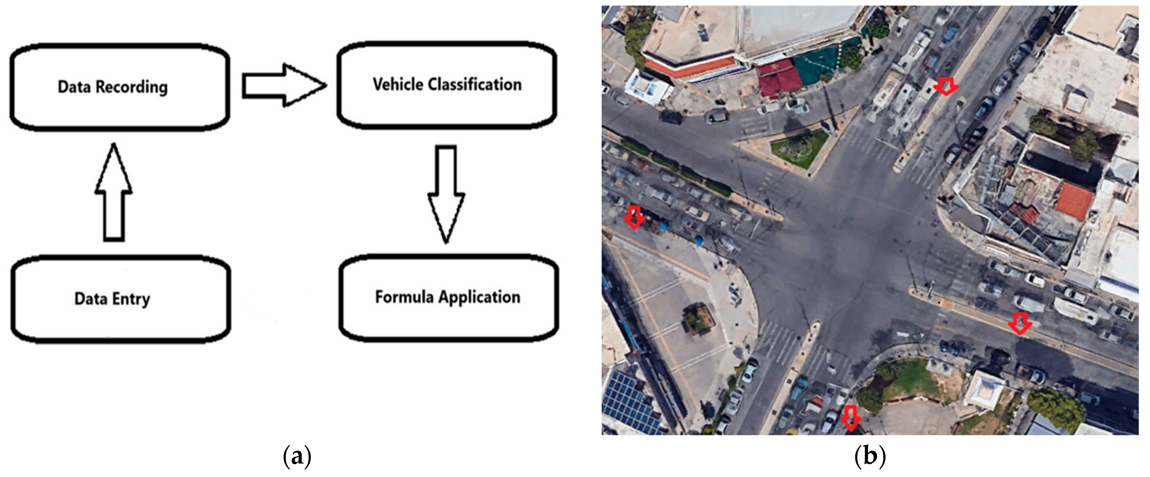
Figure 2.
Intersection of Iera Odo-Thivon (a) and Lane Grouping of the Experimental Process (b).
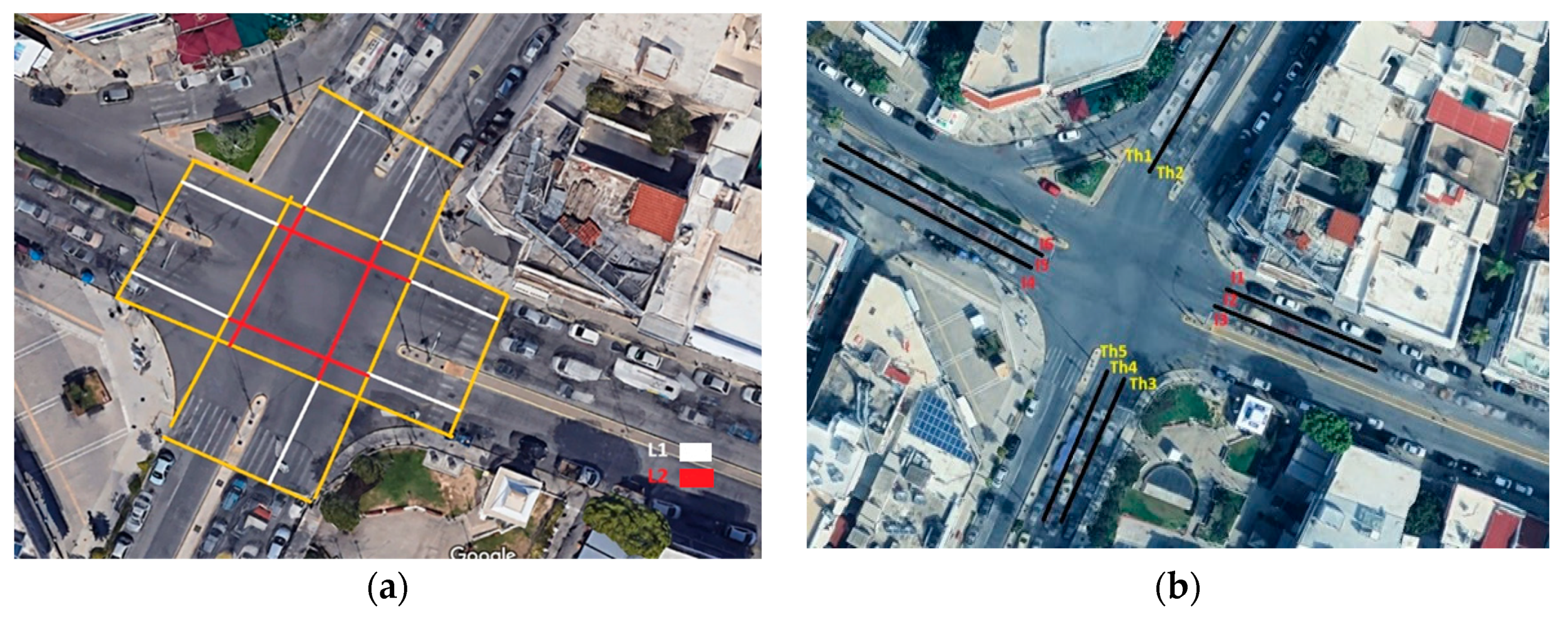
Figure 3.
Rate (%) of pollutant mass emissions during working days, for small vehicles with benzine-engine (a), medium vehicles with benzine-engine (b), small vehicles with diesel-engine (c) and medium vehicles with diesel-engine (d).
Figure 3.
Rate (%) of pollutant mass emissions during working days, for small vehicles with benzine-engine (a), medium vehicles with benzine-engine (b), small vehicles with diesel-engine (c) and medium vehicles with diesel-engine (d).
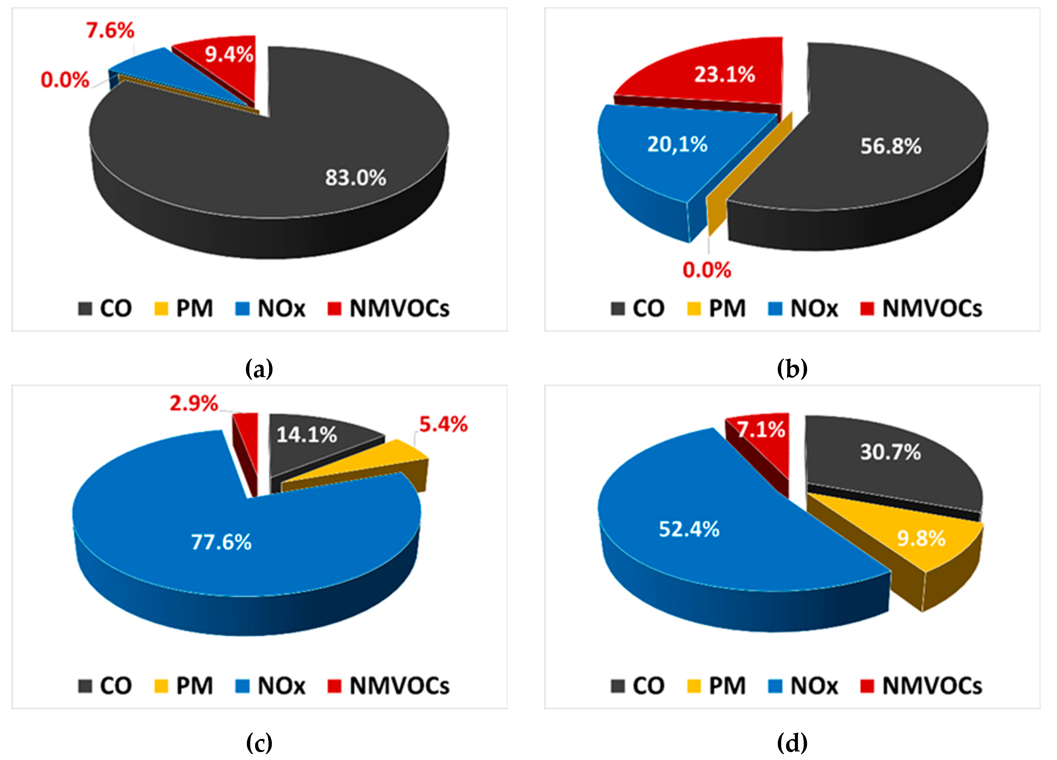
Figure 4.
Rate (%) of pollutant mass emissions during non-working days, for small vehicles with benzine-engine (a), medium vehicles with benzine-engine (b), small vehicles with diesel-engine (c) and medium vehicles with diesel-engine (d).
Figure 4.
Rate (%) of pollutant mass emissions during non-working days, for small vehicles with benzine-engine (a), medium vehicles with benzine-engine (b), small vehicles with diesel-engine (c) and medium vehicles with diesel-engine (d).
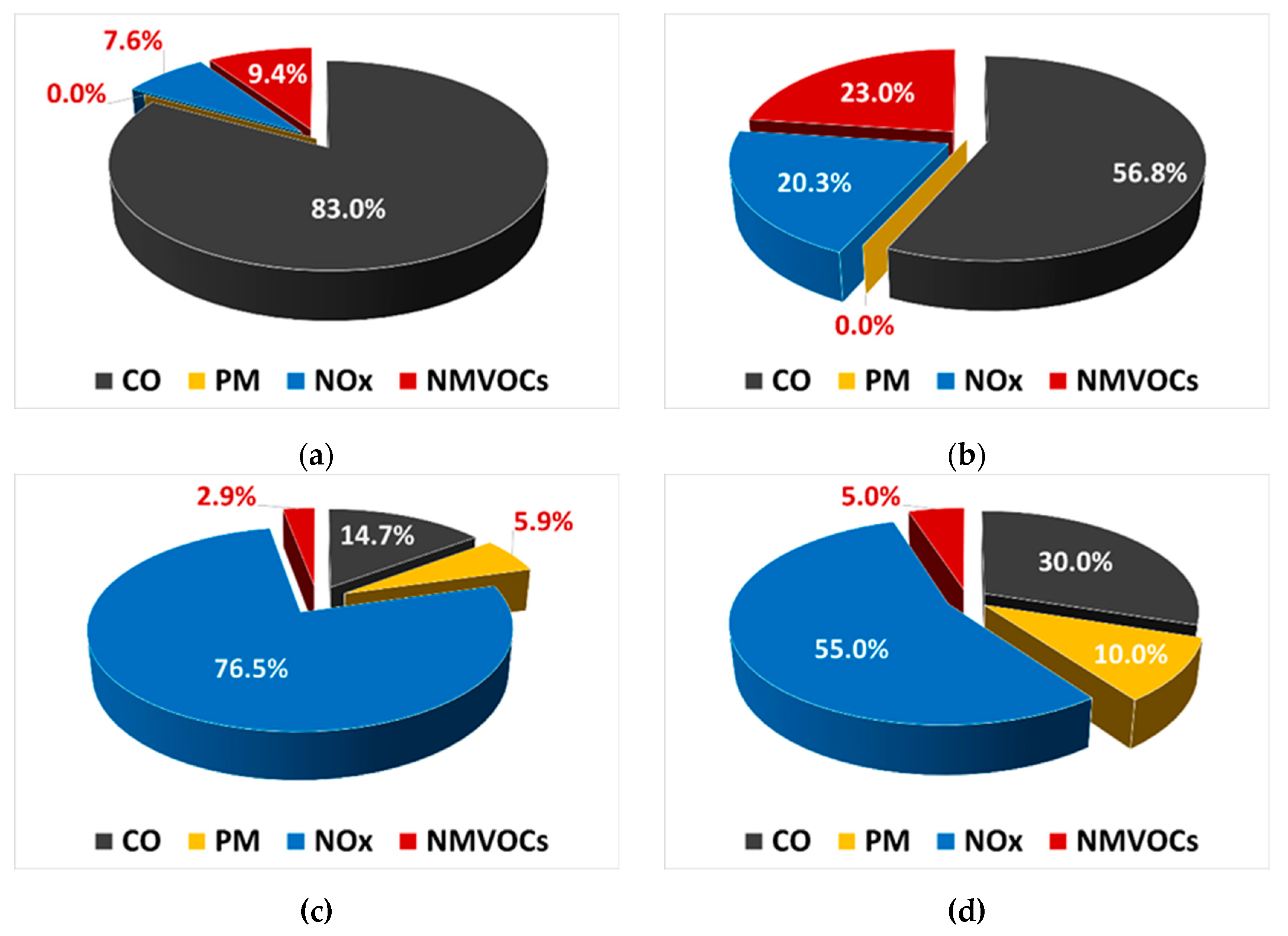
Figure 5.
Total emitted pollutant’s’ mass (sum of CO, PM, NOX and NMVOCs) by each vehicle type during working and non-working days.
Figure 5.
Total emitted pollutant’s’ mass (sum of CO, PM, NOX and NMVOCs) by each vehicle type during working and non-working days.
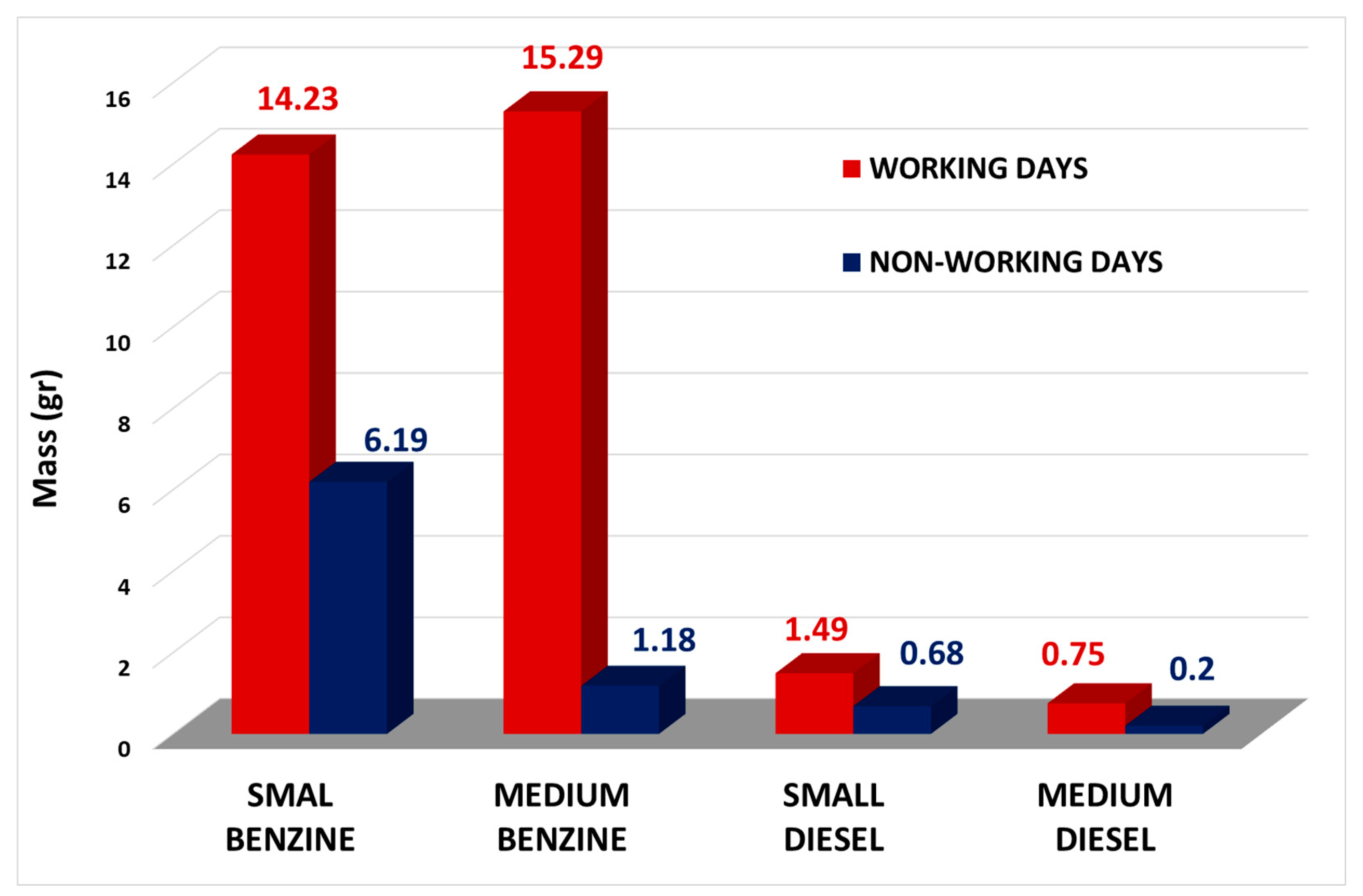

Table 1.
Data Collection.
| Date | Time | Weather Conditions | Temperature(°C) | |
|---|---|---|---|---|
| 1st | 18.12.2023 | 07:30-08:00 am | Light cloud cover with sunshine. | 8 |
| 2nd | 22.12.2023 | 05:30-06:00 pm | Light cloud cover/Sunset. | 12 |
| 3rd | 08.01.2023 | 07:30-08:00 am | Light cloud cover without sunshine. | 7 |
| 4th | 14.01.2023 | 07:30-08:00 am | Light cloud cover with minimal sunshine. | 6 |
Table 2.
Parameters, Descriptions, Equations and Units.
| Parameter | Description | Equation/Values |
|---|---|---|
| L1 | Distance from the stop line to the 1st Conflict Point of the intersection. | (m) |
| L2 | Distance from to the 1st Conflict Point to the end of the intersection (2nd Conflict Point). | (m) |
| Cij | Lane capacity: maximum number of vehicles passing during one signal cycle, Where represents the seconds during which the traffic signal indication lasts,and c represents the total number of recorded signal phases. |
|
| Sij | Saturation flow rate for lane i during signal phase j. |
|
| Saturation flow rate depending on lane width. | lane widths between: 0–2.9m:=1.736-1.752 3-3.6m:=1.815-1.830 3.7-4m:=1.898-1.913 |
|
| Adjustment factor for lane width. |
Up 3.5m =0.96, >4m =1 | |
| N |
Number of vehicles passing through each signal phase per lane. |
- |
| Number of vehicles overtaking a parked vehicle. | - | |
| Adjustment factor for lane gradient. | , road slope(degrees) | |
| Adjustment factor for the effect of parked vehicles. |
|
|
| Adjustment factor for the effect of public transportation (not considered in this study). |
|
|
| & | Adjustment factor for the effect of right-turning and left-turning vehicles. |
, = , = |
Table 3.
Correction factor rv[V(t)].
| Vi (km/h) | rV[V(t)] |
|---|---|
| 5 | 1.4 |
| 10 | 1.35 |
| 15 | 1.3 |
| 20 | 1.2 |
| 25 | 1.1 |
| 30 | 1.0 |
| 35 | 0.9 |
| 40 | 0.75 |
| 45 | 0.6 |
| 50 | 0.5 |
| 60 | 0.3 |
Table 4.
Average vehicle emissions per kilogram of fuel consumed (g/kg).
| Pollutant | Small Benzine | Medium Benzine | Small Diesel | Medium Diesel |
|---|---|---|---|---|
| PM | 0.02 | 0.04 | 0.8 | 2.64 |
| CO | 49 | 84.7 | 2.05 | 8.19 |
| NOx | 4.48 | 29.89 | 11.2 | 13.88 |
| NMVOCs | 5.55 | 34.42 | 0.41 | 1.88 |
Table 5.
Average fuel consumption per vehicle type (Lit/km).
| Small Benzine |
Medium Benzine |
Small Deisel |
Medium Deisel |
|---|---|---|---|
| 0.06 | 0.08 | 0.05 | 0.07 |
Table 6.
Average vehicle emissions (g/km).
| Pollutant | Small Benzine | Medium Benzine | Small Diesel | Medium Diesel |
|---|---|---|---|---|
| PM | 0.00 | 0.00 | 0.04 | 0.16 |
| CO | 2.18 | 5.01 | 0.09 | 0.50 |
| NOx | 0.20 | 1.77 | 0.49 | 0.86 |
| NMVOCs | 0.25 | 2.04 | 0.02 | 0.12 |
Table 7.
Estimated emitted mass (gr) of PM.
| Benzine | Diesel | |||
|---|---|---|---|---|
| Small vehicles | Medium vehicles | Small vehicles | Medium vehicles | |
| Working day | 0.00 | 0.00-0.01 | 0.05-0.10 | 0.05-0.10 |
| Non-working day | 0.00 | 0.00 | 0.04 | 0.02 |
Table 8.
Estimated emitted mass (gr) of CO.
| Benzine | Diesel | |||
|---|---|---|---|---|
| Small vehicles | Medium vehicles | Small vehicles | Medium vehicles | |
| Working day | 10.84-12.40 | 6.14-12.96 | 0.15-0.25 | 0.17-0.31 |
| Non-working day | 5.14 | 0.84 | 0.10 | 0.06 |
Table 9.
Estimated emitted mass (gr) of NOX.
| Benzine | Diesel | |||
|---|---|---|---|---|
| Small vehicles | Medium vehicles | Small vehicles | Medium vehicles | |
| Working day | 0.99-1.13 | 2.17-4.57 | 0.80-1.39 | 0.29-0.53 |
| Non-working day | 0.47 | 0.30 | 0.52 | 0.11 |
Table 10.
Estimated emitted mass (gr) of NMVOCs.
| Benzine | Diesel | |||
|---|---|---|---|---|
| Small vehicles | Medium vehicles | Small vehicles | Medium vehicles | |
| Working day | 1.23-1.40 | 2.49-5.27 | 0.03-0.05 | 0.04-0.07 |
| Non-working day | 0.58 | 0.34 | 0.02 | 0.01 |
Disclaimer/Publisher’s Note: The statements, opinions and data contained in all publications are solely those of the individual author(s) and contributor(s) and not of MDPI and/or the editor(s). MDPI and/or the editor(s) disclaim responsibility for any injury to people or property resulting from any ideas, methods, instructions or products referred to in the content. |
© 2025 by the authors. Licensee MDPI, Basel, Switzerland. This article is an open access article distributed under the terms and conditions of the Creative Commons Attribution (CC BY) license (http://creativecommons.org/licenses/by/4.0/).
Copyright: This open access article is published under a Creative Commons CC BY 4.0 license, which permit the free download, distribution, and reuse, provided that the author and preprint are cited in any reuse.


