
Submitted:
21 March 2024
Posted:
22 March 2024
You are already at the latest version
Abstract
This work presents a novel approach for the study of the movement of droplets on inclined surfaces under the influence of gravity and chemical heterogeneities. The developed numerical methodology uses data-driven modeling to extend the applicability limits of an analytically derived reduced-order model for the contact line velocity. More specifically, while the reduced-order model is able to capture the effects of the chemical heterogeneities to a satisfactory degree, it does not account for gravity. To alleviate this shortcoming, datasets generated from direct numerical simulations are used to train a data-driven model for the contact line velocity, which is based on the Fourier neural operator and corrects the reduced-order model predictions to match the reference solutions. This hybrid surrogate model, which comprises of both analytical and data-driven components, is then integrated in time to simulate the droplet movement, offering a speedup of five orders of magnitude compared to direct numerical simulations. The performance of this hybrid model is quantified and assessed in different wetting scenarios, by considering various inclination angles and values for the Bond number, demonstrating the accuracy of the predictions as long as the adopted parameters lie within the ranges considered in the training dataset.
Keywords:
wetting hydrodynamics
; droplet transport
; reduced-order modeling
; machine learning
; Fourier neural operator
1. Introduction
The motion of droplets is a phenomenon that most people encounter in their everyday lives, either in the form of vapor condensation on a cold window, water spilling on leaves during the watering of plants, etc. It is also a phenomenon that is relevant to many applications; from microfluidic lab-on-a-chip devices that can process a large number of microscopic chemical or biological samples [1], to coating and 3D printing [2]. For these reasons, there is a great need to understand and control droplet motion in these and many other applications [see 3, for a review].
From a modeling perspective, the most intricate aspect of a moving droplet is the description of the multiscale physical processes affecting the contact line dynamics, which originate from the molecular interactions at the nanoscale. The contact line is defined as the line on the periphery of a droplet, separating the solid, liquid and gas phases. The associated local contact angle is the angle formed between the solid-liquid and the liquid-gas interfaces and is typically dictated by the chemistry of the surface and may exhibit spatial variations and features due to unavoidable randomness on a natural surface or deterministic by surface design. A solid surface is considered hydrophilic when a fully equilibrated droplet assumes angles that are smaller than , and hydrophobic when these are larger than . When the droplet is in motion, what we observe macroscopically is that the apparent contact angle is different from the local one, causing the displacement of the contact line. In surfaces with no hysteresis effects, the droplet reaches equilibrium when both the local and apparent contact angles along the contact line match.
The focus of this study is the modeling of droplet motion on inclined, chemically heterogeneous surfaces. This specific setting is very relevant to water harvesting, with numerous examples in nature and relevant bio-inspired applications [4]. Droplets are typically observed to remain stationary on the inclined surface up to a critical inclination angle, beyond which the droplet moves downhill as it is able to overcome the surface heterogeneities be they natural or artificial. For larger inclination angles, instabilities may develop, leading to the formation of cusps and even droplet breakup [5,6]. The impact of structured surface heterogeneities has also attracted interest in recent years, especially with the advent of specialized surface fabrication technologies. Several experimental studies focused on uncovering the influence of heterogeneous features on the critical inclination angle and the subsequent dynamic sliding behaviour [7,8,9,10,11,12]. Going even further, Varagnolo et al. [13] studied the influence of the shape of the hydrophobic regions, suggesting practical criteria for surface designing in order to tune the static and dynamic behavior of droplets. In more “exotic” applications, researchers were able to make droplets run uphill either with a heterogeneity gradient opposing the gravity field [14], or with vibrations [15]. Moreover, approaches based on mathematical modelling and analyses were also utilized to study idealized geometries, typically adopting simplifying assumptions [16,17] which limited their applicability in more realistic scenarios.
Thus, numerical modelling emerges as an attractive alternative approach to go past the limitations of analytical results and mitigate the need for specialized equipment for accurate experiments. Numerical studies, however, also adopt different approaches. For example, lubrication-type models that are derived as approximations of the Navier–Stokes equations and apply for small contact angles and negligible inertia, have been employed to study droplets on inclined surfaces, with or without chemical heterogeneities [18,19,20,21]. Moreover, Afkhami et al. [22] conducted direct numerical simulations (DNS) to study forced dewetting, comparing their results against Cox’s contact line velocity model [23]. Relevant computational fluid dynamics (CFD) studies emerged, studying various wetting hydrodynamic settings for realistic apparent contact angles [24,25,26,27,28]. Other numerical approaches include Lattice–Boltzmann methods [29,30,31], phase-field methods [32,33], and to a lesser extend molecular dynamics [34,35], and smooth particle hydrodynamics [36]. Even though these numerical approaches offer a reliable alternative to costly experiments, they are typically associated with a high computational cost and significant runtime.
The astounding uptake of data-driven methods in science and engineering has showcased the potential to accelerate numerical solutions in different disciplines. Specifically for fluid dynamics [37], common examples of enhancing the solution efficiency through data-driven methods include turbulence modelling through Reynolds averaged Navier–Stokes and large eddy simulations [38,39] and super-resolution, where coarse simulations are processed by data-driven models to infer the solution to higher resolution grids [40,41,42]. Another promising approach is the construction of hybrid surrogate models, which combine data-driven and reduced-order models. Characteristic examples of this approach are two works that developed surrogate models for the prediction of the kinematics of spherical particles [43] and bubbles [44], as well as the recent study by the present authors for the dynamics of thin droplets on heterogeneous surfaces without gravity [45]. With this kind of hybrid modelling, the data-driven component of the model learns to correct and extend the applicability of an analytically derived reduced-order model using the full simulation data as a reference solution. This approach demonstrated improved agreement with the reference solution compared to the base reduced-order model, expanding its regime of applicability to tackle more complex scenarios, and also exhibited better generalizability compared to fully data-driven models.
Specifically, the aforementioned study by Demou and Savva was a proof-of-concept study in which a hybrid analytical/data-driven modelling approach was utilized for the first time in the context of wetting hydrodynamics, which was based on training datasets that were efficiently generated for lubrication-type models [45]. In the limit of thin droplets, the asymptotic theory of Lacey [46] applies, which provides a reasonably accurate estimate for the normal component of the contact line velocity. Although higher-order corrections to this result have been obtained via analytical means [47], this study demonstrated that the data-driven route is also applicable, especially for cases where improving upon a simplified low-order model becomes a formidable challenge. Within this approach, the hybrid model for the contact line velocity consists of the superposition of Lacey’s model and its data-driven counterpart, which was then evolved using the method of lines with a standard ordinary differential equation (ODE) solver. The model was shown to considerably shorten simulation times compared to a full numerical simulation, and to be able to capture the dynamics accurately even for heterogeneity profiles that were very different from the heterogeneity profiles seen during training.
The present work expands upon this modelling framework to describe the dynamics of droplets that are driven by the interplay of chemical heterogeneities and the gravitational force, using (i) full DNS datasets and (ii) a reduced-order model which is based on the theory of Cox [23] which does not explicitly account for the effects of gravity, so that they are entirely accounted for by the data-driven model. In Section 2, the mathematical and numerical framework used to generate the datasets and train the data-driven model is described. This is followed by the presentation of the results of this study, including the testing of the hybrid surrogate model in different settings in Section 3. Finally, Section 4 concludes this study with a summary of the key results.
2. Governing Equations and Numerical Methods
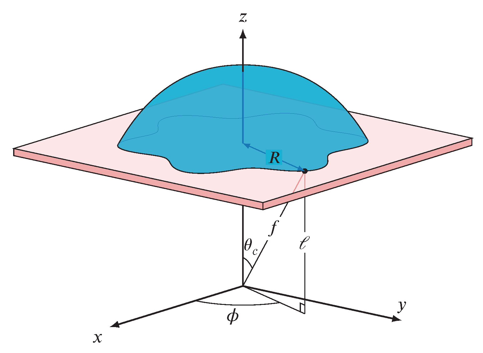
The goal of this study is to train data-driven models to predict the droplet dynamics for a system that is schematically shown in Figure 1. More specifically, a liquid droplet with density and viscosity , which is surrounded by a gas phase with corresponding properties and (hats denote dimensional quantities), slides under the influence of gravitational acceleration over a chemically heterogeneous surface with inclination angle . The surface tension of the two-fluid interface, and the chemical character of the substrate, as expressed through the local contact angle , influence the dynamic behaviour of the droplet and its shape. Considering the case set-up, the relevant dimensionless groups are the Reynolds number , characterizing the relative influence of inertial over viscous effects, the capillary number , characterizing the relative influence of viscous over capillary effects, and the Bond number, , for capturing the relative importance of gravity to surface tension. In these dimensionless groups, is the characteristic length scale taken to be the domain size, and is the characteristic velocity scale.
To generate the training dataset, a number of DNS cases are run and the evolution of the contact line is extracted under different conditions. In all cases, an initially hemispherical droplet of radius 0.125 was placed on a solid surface at the bottom of a box, with open boundaries everywhere else. The density and viscosity ratios between the two fluids were set to 0.1, and Reynolds and Capillary numbers to , . The surface inclination angle and the Bond number were varied within , and respectively. Furthermore, the initial position of the droplet and the heterogeneity profile on the inclined substrate were also varied, with more details provided in Section 3. The following paragraphs provide a description of the mathematical and numerical framework used to generate the datasets and train the data-driven models.
2.1. Governing Equations for DNS
The governing equations for the wetting scenarios considered are the two-phase Navier–Stokes equations, including the effects of surface tension and gravity. The two different fluids (resembling a liquid and a gas) are differentiated with a colour function [48]. Considering that volume is occupied by fluid (1) and by fluid (2), with boundaries and , respectively, the colour function is defined as
with the interface between the two fluids denoted by , which is the part of the boundary that is common to both regions. The physical fluid properties in the whole domain can be obtained as a weighted average between the fluid properties of each phase,
where is the value of a relevant property in the entire domain and subscripts “1” and “2” indicate the property values in each phase.
Within this setting, the governing equations are recast in dimensionless form as,
The density and viscosity are made dimensionless using the corresponding values of fluid (1), while the pressure scale is taken as . The two-fluid interface is characterised by a unit normal vector , a delta function centered on the interface located at , , and a local surface curvature .
The open source code Basilisk ([49,50,51]) is utilized to solve equations (3), subject to appropriate boundary and initial conditions (described in Section 3). Basilisk specializes in solving partial differential equations on adaptive Cartesian meshes. The dynamics of the two-fluid interface (Equation (3b)) is captured by a conservative, non-diffusive geometric volume-of-fluid method. The chemical heterogeneities on the inclined substrate are expressed through the local contact angle, which is implemented numerically using height functions [52,53]. The discretization of viscous forces follows an implicit formulation, while the surface tension forces are modelled using the continuous surface force method [54]. The resulting Poisson equation for the pressure is solved with a build-in iterative multigrid solver. To further increase the efficiency of the solution, Basilisk provides the option of using adaptive mesh refinement, based on customized criteria. In the context of the present study, it is desired to maintain a higher spatial resolution in the vicinity of the two-fluid interface, compared to less active regions. This leads to obtaining accurate solutions on a discretized domain with significantly less grid nodes. The code was extensively validated in a variety of multiphase flow problems (see http://basilisk.fr/) and is widely used in contact line studies (see, e.g., [27,55,56]).
2.2. Reduced-Order Model
In the limit of negligible inertia and small Ca, Cox developed an asymptotic model for the velocity normal to the contact line [23], in the form
where and are the apparent and local contact angles, respectively,
and
In Equation (4a), is the azimuthally averaged droplet radius, and in Equation (4c) is the viscosity ratio between the two fluids. In this formulation, is derived from the solution to the Young–Laplace equation for specified contact line shape.
In Cox’s approach, was based on an asymtptotic expansion into the vicinity of the contact line by assuming a wedge-like geometry, with the details of the dynamics in the bulk of the droplet and the dynamics of the entire flow field in the vicinity of the contact line being encoded by the parameters and , respectively. These, in addition to the parameter , which corresponds to the slip length, were fitted to the DNS data to best approximate the output of the simulations. To that end, four preliminary simulations were carried out, describing the spreading of an initially hemispherical droplet on homogeneous substrates with local contact angles of , , , and , which span a broad spectrum of local contact angles. The simulations were conducted for 3 dimensionless time units, within which the droplets spread on the substrate, but are still far from equilibrium so that contact line velocities do not become vanishingly small. For carrying out the fitting of DNS data with equation (4a), an explicit expression for is used (see Equation (A13)), and contact line snapshots were collected at intervals of 0.1 dimensionless time units. Using least-squares fitting for the contact line velocity, the values obtained were , and , with a mean relative deviation , where is the total number of contact line snapshots considered. These parameters were held constant for all tests presented in this study.
The only difficulty in using Equation (4) for chemically heterogeneous substrates is the calculation of the apparent contact angles . To overcome this bottleneck, an approximation to the contact angle model is obtained in Appendix A, see Equation (A16). This model is based on a perturbation expansion to the Young–Laplace equation, assuming a spherical and a circular contact line at leading order, and it naturally deviates from the expected solution as the contact line deformation becomes larger (see Figure A3 for the mean absolute error estimation). Nonetheless, due to the parameter ranges considered in the present study (described in Section 3), contact line deformations are generally weak and the approximate contact angle model yields sufficiently accurate results to be used for the training of the data-driven models.
2.3. Data-Driven Method
The aim of the data-driven modeling procedure is to approximate a mapping between an input and an output function space, i.e. , where is an instance of the input function space, is an instance of the output function space, and are the model parameters. Kovachki et al. [57] presented a formulation based on neural operators, approximating this mapping as,
Within this approach, the input is first lifted to a higher parameter space with operator . Then, a local linear operator and an integral kernel operator are applied, followed by the activation function . This last operation is applied L times with different and operators, before operator projects the output back to the solution space. Choosing Fourier transforms to construct the integral kernel operators, leads to the Fourier neural operator (FNO) architecture [58], where each operator called a Fourier layer, and
In the above expression, operator transforms the input to the Fourier space, where the weights of the Fourier modes are learned during training. Then, the inverse Fourier transform transforms the result back to the physical space. Overall, the model parameters consist of the elements of , , and , for . Figure 2 shows a schematic representation of the FNO architecture, and the interested reader is referred to the contribution by Li et al. [58] for more details.
The role of FNO-based models in the present work is correcting Cox’s reduced-order model presented in Section 2.2 in order to approximate the DNS solution. As previously mentioned, this approach is an extension of a previous work by Demou and Savva [45] that developed a data-driven workflow for wetting hydrodynamics in the limit of very small apparent contact angles, without gravity effects. In the referred study, the data-driven model provided higher order corrections to the reduced-order model. These corrections were approximately independent from the chemical heterogeneities on the substrate, leading to data-driven models were able to generalize well even for cases with significantly different heterogeneity profiles. A different approach is required in the present study because the droplets migrate mainly due to the gravity force, but their movement is also affected by the presence of the chemical heterogeneities on the substrate. As the effects of gravity are not incorporated in Cox’s reduced-order model, the developed data-driven model will focus on correcting Cox’s predictions with respect to the gravity induced translation motion. Therefore, the trained model will provide the correction to the first Fourier harmonic of the velocity normal to the contact line (i.e. translational droplet motion) and will be combined with Cox’s reduced-order model for the prediction of the higher Fourier harmonics (i.e. droplet spreading).
More specifically, the inputs to the data-driven model are the physical space representation of the first Fourier harmonics of the apparent contact angle, , the local contact angle, , which are essentially low-pass filters of and , and the gravity component which is approximately normal to the contact line, . All three inputs are functions of the azimuthal angle, , that parametrizes the contact line in a moving coordinate system centred at the centroid of the wetted area. The output of the model is expected to approximate the first Fourier harmonic of the difference between the velocities normal to the contact line as predicted by the DNS and the reduced-order model, . The model is trained with contact line snapshots from the DNS cases, therefore the training error is defined as,
where, is the output of the data-driven model and is the corresponding reference solution. The testing error, , is similarly estimated using samples. In all snapshots considered in the training and testing datasets, the DNS solution and Cox reduced-order model prediction never exactly match. Therefore, , which quantifies their difference, never vanishes and the summands in Equation (7) never diverge. This is even true for DNS snapshots for which the droplets are at equilibrium, since, due to the estimation errors in the contact angle, does not vanish. Once the data-driven model is successfully trained, the data-driven velocity predictions are added to the predictions of Cox’s reduced-order model to form the hybrid contact line velocity model, . This hybrid model is then used to evolve the solution in time using standard time integration schemes that are typically adopted for the numerical solution of ODEs.
Many variations of the training procedure described above were tested in order to identify the best available approach to model droplet dynamics on inclined heterogeneous surfaces. These preliminary training approaches included (i) different forms of the loss function, (ii) different activation functions, (iii) retaining more Fourier harmonics in the input and output of the AI model, (iv) including the contact line shape and the gravity component normal to the inclined substrate as input to the AI model, among other attempts. The training procedure described above emerged as the best approach that balances both accuracy and robustness in predicting the future state of a moving droplet in the wide range of tests presented in Section 3.
2.4. Error Measure Based on the Fréchet Distance
The accuracy of the developed model must be assessed on its ability to predict the contact line position at a given time, a measure that is not provided by Equation (7) as it is based on the difference between the predicted and reference contact line velocities. Therefore, a more relevant error measure is utilized, defined at any specific time instance of a simulation as,
Here, and are the contact line positions as predicted by the AI and the DNS at time t respectively, and is the Fréchet distance, characterising the similarity between two curves [59]. This similarity measure takes into account both the location and ordering of the points along the curves. By normalizing the Fréchet distance with a characteristic diameter (derived from the area of the wetted region), this error measure becomes equal to 100% for two externally tangent circles of the same radius. In the following sections, the progress of the training and testing of the data-driven models is quantified using and (defined in Equation (7)), while the model performance in accurately predicting the contact line position in representative demonstration cases is quantified using at specific times.
3. Results
3.1. Modeling Parameters
All DNS cases consider a single droplet moving on a chemically heterogeneous inclined surface, in a setup that is illustrated in Figure 1. As mentioned in Section 2, the computational domain is a box, with the solid surface at the bottom and open boundaries everywhere else. An initially hemispherical droplet of radius 0.125 was placed with the center of its contact line at some random location towards the middle upper half of the domain, where and . The gravity field was given by , where and are the unit vectors along the y- and z-directions, and . The density and viscosity ratios between the two fluids are set to 0.1. Considering the scales introduced in Section 2.1, the adopted values for the dimensionless groups are , and , where the Bond number varies randomly to produce different values for g. These dimensionless groups were selected instead of the arguably more physical choice of employing droplet-based dimensionless groups using, e.g., the initial droplet radius and the contact line velocity as the length and velocity scales, leading to Red, Cad, and Bod, because the contact line velocity is not available a priori. Scrutinizing the simulations, a typical contact line velocity is in the order of 0.01, leading to droplet-based dimensionless groups in the order of , and . Considering the small Cad and Bod values, it is expected that the droplets will assume weakly perturbed spherical cap shapes as they slide on the inclined surface, such that the approximate contact angle model in Equation (A16) can provide reliable estimates.
The bottom surface assumes heterogeneity profiles generated by the multiparameter function
where and . Parameters are uniformly distributed random numbers within the ranges,
A similar function was also adopted in our previous study [45], validating that the rich distribution of heterogeneity profiles enhances the diversity of the training samples that will be subsequently used for the data-driven model training.
As mentioned in Section 2.1, the simulations were carried out with Basilisk, using a Courant–Friedrichs–Lewy (CFL) criterion of CFL=0.8, and an adaptive Cartesian grid that is dynamically modified in the visinity of the two-fluid interface. More specifically, the grid is locally refined or coarsened in an octree structure, by monitoring the discretisation error of the indicator function C, as estimated by wavelet transforms. The present study adopted maximum and minimum grid spacing values of and respectively. To verify the accuracy of the solutions with such a grid, Figure 3 shows a comparison against a higher resolution grid with and . Even though the higher resolution simulations used 4 times more CPU cores, the wall time was approximately 6 times longer compared to the lower resolution simulations. Nonetheless, the final solutions predicted with the two different grids are in satisfactory agreement, with an error based on the Fréchet distance of 4.8% after 60 dimensionless time units. This small deviation highlights the fact that, with and the available computational resources can be efficiently utilised to generate a significant sample size, without a considerable adverse effect on the solution accuracy.
Overall, 160 DNS cases were carried out for an average duration of 50 dimensionless time units. Cases that either reached the domain boundaries or got pinned on the heterogeneity patterns were ended prematurely, while cases that still exhibited droplet movement far from the boundaries were run beyond 50 time units. These simulations provided over 80,000 snapshots, taken at intervals of 0.1 dimensionless time units, to be used as training and testing samples. Each snapshot was post-processed to extract the contact lines and parametrise them in terms of 128 uniformly distributed points along the azimuthal direction . These contact line profiles were subsequently used to calculate: (i) the velocities normal to the contact line using finite differences, (ii) the local contact angles along the contact line from Equation (9), i.e. , and (iii) the apparent contact angles from Equation (A16). Overall, each sample (corresponding to a snapshot in time) comprised of
- input data: , where the last term corresponds to the component of the acceleration of gravity on the -plane which is approximately normal to the contact line, and
- target data:
In total, 64,000 samples were used for training (i.e. 80% of the total sample size) and the remaining 16,000 for testing. The training lasted for 500 epochs, adopting a Rectified Linear Unit (ReLU) as the activation function, a batch size of 20 samples, and an initial learning rate of , which was halved every 50 epochs. Taking advantage of the use of Fourier transforms, the trained model was structured to retain only the first Fourier harmonic which can be interpreted as providing corrections to Cox’s reduced order model only for the translation motion of the droplet, as opposed to local spreading which is expected to be captured by Cox’s model fairly accurately. The remaining FNO hyperparameters, i.e. the width w of the channel space after the application of the lifting operator , and the number of Fourier layers (see Figure 2), were tuned after a series of preliminary experiments, considering values and . Table 1 presents the testing errors for all these preliminary trained models, revealing that the values and , lead to the best performing model, with 173,121 learning parameters. Adopting the best performing set of hyperparameters, Figure 4 shows the evolution of the training and testing errors as a function of the training epochs, considering two different sample sizes. The final testing error for the smaller sample size is 16.4%, approximately 1.5% larger than the larger sample size. This observation suggests that further increasing the sample size will only have a small impact on the model accuracy. Admittedly, such testing errors may appear relatively large in the context of data-driven surrogate models. Nonetheless, the role of this data-driven model is to correcting an existing reduced-order model which, in some cases, provides predictions that are close to the target solution, with very small correction margins and, therefore, large relative errors.
Figure 5, shows the velocity contributions from the reduced-order model and the data-driven model, as well as a comparison between the overall model prediction and the reference DNS solutions for two cases, considering the same Bond number but different inclination angles. For reference, the droplet trajectories for these two cases and heterogeneity profile are depicted in Figure 8(a) and (c). As clearly shown, in these two cases the reduced-order model cannot predict the large-scale translational motion of the droplet, as explained in Section 2.3. This observation provided the motivation to combine the reduced-order model, which describes the spreading motion relatively accurately, with an AI model that focuses on the translational motion and does not interfere with spreading. As expected, the reference contact line velocities in the large inclination angle case are significantly larger than the small inclination angle case, requiring the AI contribution to bridge the gap between reduced-order model and the DNS solution. In both cases, the predictions of the overall model follow the DNS solution closely, which can be used in a method-of-lines time integration procedure to predict the droplet position in time. Within this framework, the whole numerical integration takes a few seconds on a typical laptop computer, as opposed to days of runtime on high-performance computing resources for the corresponding DNS run, amounting to a speedup of at least five orders of magnitude.
3.2. Tests
To assess the accuracy of the hybrid surrogate model in different wetting scenarios, this section presents a series of test cases adopting heterogeneities that were not encountered during training. First, Figure 6 shows comparisons between the hybrid surrogate model predictions and the corresponding DNS solutions for different heterogeneity profiles, considering and . Figure 6(a) uses a homogeneous profile with , while panels (b) and (c) of the same figure assume profiles that are defined by specific parameter choices in Equation (9). For the homogeneous case, Cox’s reduced-order model plays a minor role in the contact line velocity prediction since the contact line quickly assumes a constant shape and the droplet descends with constant speed throughout the simulation. Hence, to a large extend, the movement of the droplet is described by the AI component of the hybrid model. The hybrid surrogate model results in a 2.9% Fréchet-based error, which attests to the capability of the AI component to provide a reliable estimation of the translation motion of the droplet, at least on simple homogeneous substrates. In Figure 6(b), the droplet experiences pinning and depinning states as it moves over the horizontal striped features, altering the contact line shape and the apparent contact angles, therefore the importance of Cox’s reduced-order model contribution is elevated. Still, in this scenario the predictions of the hybrid surrogate model exhibit an error as low as 4.8% compared to the reference DNS solution. Finally, Figure 6(c) exhibits a case where the droplet is quickly pinned due to the configuration of the chemical heterogeneities, in which case the hybrid surrogate model excellently reproduces the dynamics. It is worth noting that in all cases presented in Figure 6, the trajectory of the centroid of the wetted area is accurately reproduced by the hybrid surrogate model.
Figure 6.
Comparisons between the predictions of the hybrid surrogate model (red lines) and DNS solutions (semi-transparent blue regions) at the final time step of the simulations . The initial conditions are also shown, centered approximately around . The trajectories of the centroid of the wetted area are shown with black and red-dashed lines for the DNS and the hybrid surrogate model solutions respectively. The heterogeneity profile in (a) assumes a uniform value of . The heterogeneity profiles in all other figures are described by Equation (9), with specific parameters, = (b) , and (c) . In all cases and . The errors based on the Fréchet distance are (a) 2.9%,(b) 4.8%, and (c) 1.1%. The background follows the same shading convention as Figure 3.
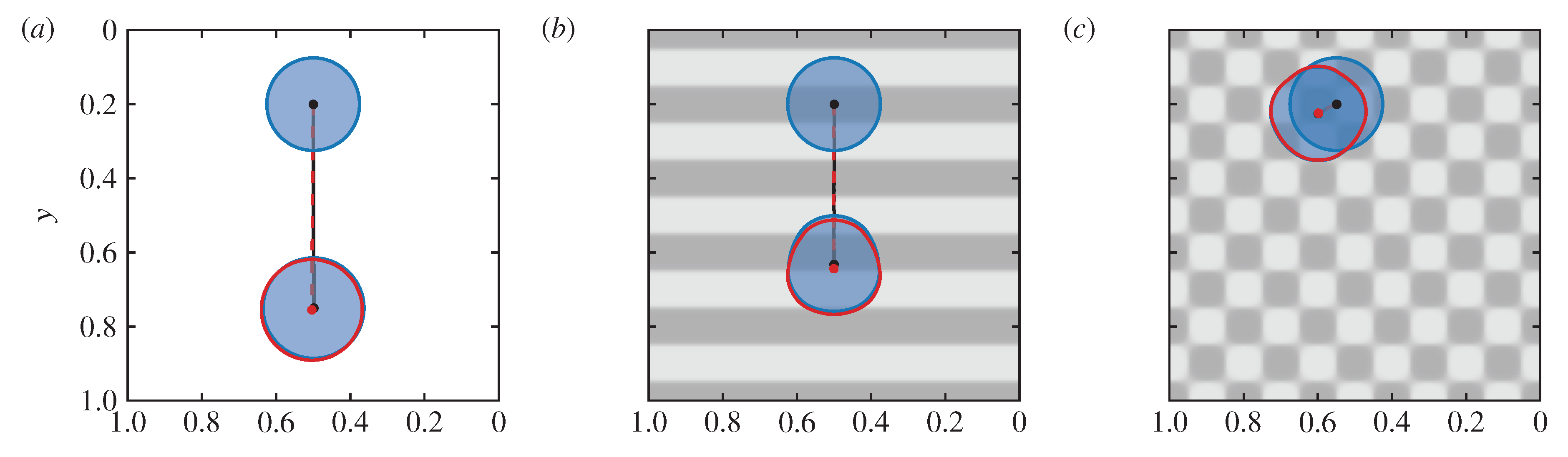
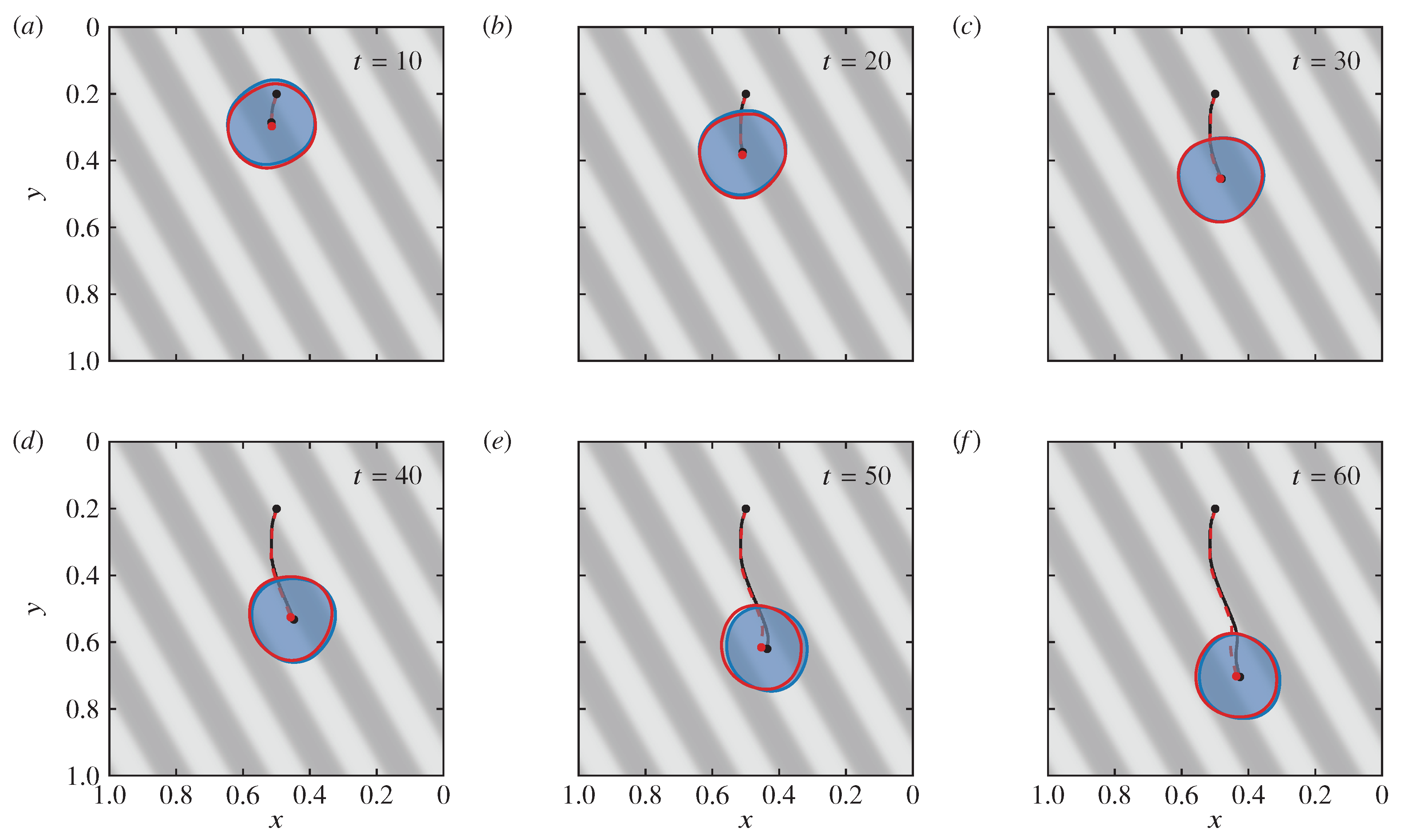
Figure 7 shows various droplet snapshots in time, for a wetting scenario with a more intricate dynamical behavior, considering the same inclination angle and Bond number as before. The presence of diagonal striped features influences the droplet descent on the inclined substrate, where the centroid of the wetted area follows a curved trajectory. Initially, the droplet shifts to the left until the contact line meets a more hydrophobic stripe (darker shaded) at the left side of the bubble, somewhere between and 20. Afterwards the droplet moves diagonally, following the stripes configuration until , when the right part of the droplet lies completely on a more hydrophobic stripe. At that point, the droplet movement aligns with the gravity force until it becomes diagonal once again. This complicated movement, where the droplet is significantly influenced by both the gravity force and the chemical heterogeneities, is accurately captured by the hybrid surrogate model, exhibiting an error of only 4.3%, compared to DNS solution at the end of the simulation.
Figure 7.
Similar to Figure 6, with different panels corresponding to different time instances. The heterogeneity profile adopted is described by Equation (9), with specific parameters, . The error based on the Fréchet distance at the final time is 4.3%.
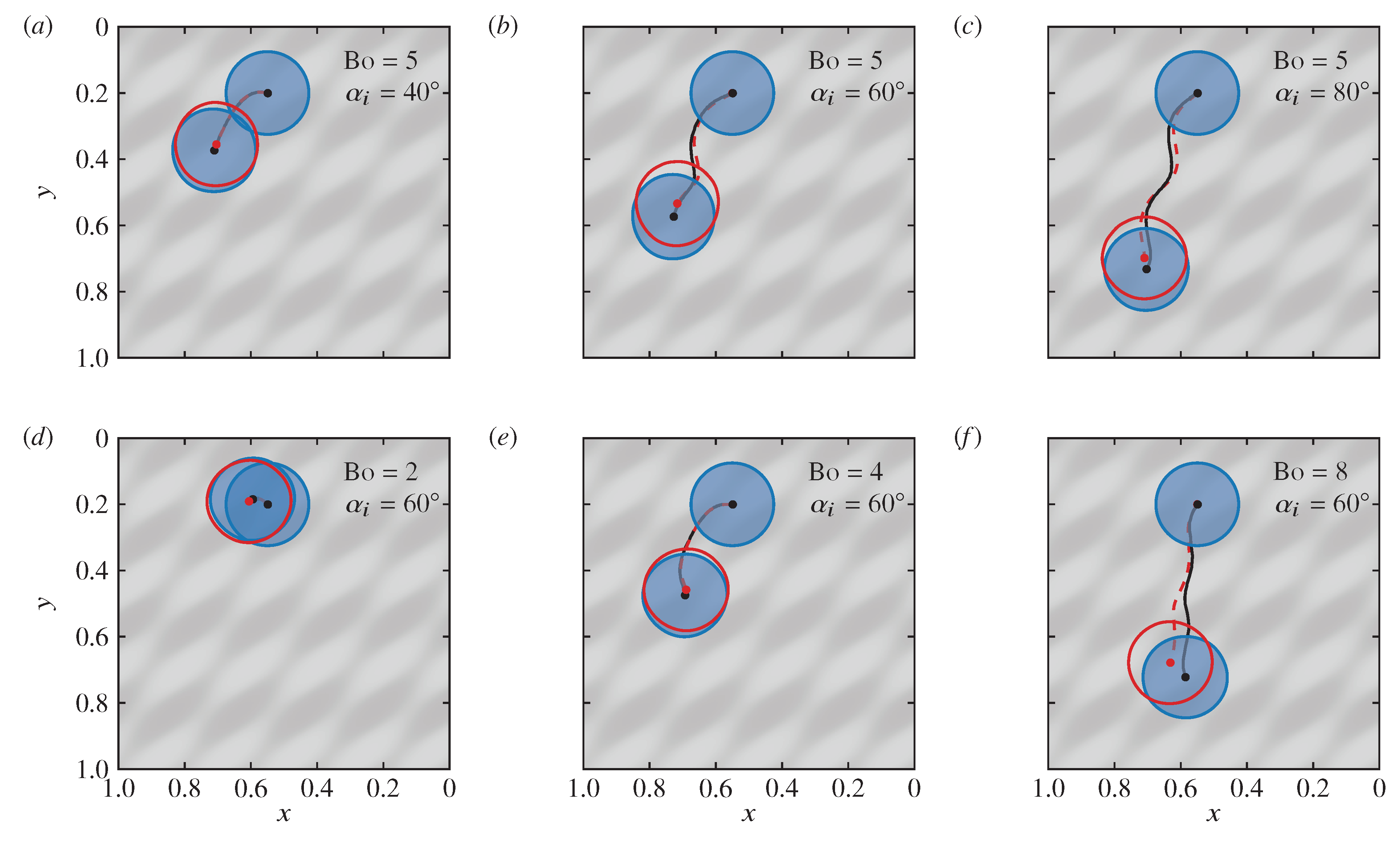
To quantify the sensitivity of the hybrid surrogate model on the characteristics of the gravity force, Figure 8 shows comparisons against DNS solutions for different values of the inclination angle and the Bond number. As expected, keeping a constant Bond number value of and increasing the inclination angle (panels (a)-(c)) increases the distance travelled by the droplet within the 80 time units considered for the simulation. Similar to Figure 7, the centroid follows a curved trajectory, guiding the droplet towards the left side, in accordance to the structure of the chemical heterogeneities. Quantifying the agreement between predicted and reference solutions, the errors based on the Fréchet distance increase from 8.2% at to 16.6% at and remain relatively unaffected to 14.1% at . Furthermore, Figure 8(d)-(f) shows cases considering a fixed inclination angle and a varying Bond number. For the lowest Bond number, the droplet barely moves and soon gets pinned on the heterogeneity features. By increasing the Bond number, the droplet is able to overcome the heterogeneity barriers and induce a downhill sliding motion, with a corresponding increase of the Fréchet-based error, noting a maximum error of 25.6% for the largest Bond number considered. A major reason behind this significant error is the that is outside the Bond number ranges used to train this model and, therefore, the data-driven model is trying to extrapolate beyond the training distribution. Another source of error is that the increasing Bond number can be thought of as an equivalent increase in g, something that influences the three-dimensional droplet shape and has an impact on the assumption of a weakly perturbed spherical cap used to develop the approximate contact angle model in Equation (A16). Overall, the errors of the hybrid surrogate model increase with increasing inclination angle and Bond numbers, while the model exhibits a satisfactory performance as long as the adopted parameters are within the ranges considered during training.
Figure 8.
Similar to Figure 6, with different panels corresponding to different values of the inclination angle and Bond number Bo. The comparison is documented at , except panel (f) where is used. The heterogeneity profile adopted is described by Equation (9), with specific parameters, . The errors based on the Fréchet distance are (a) 8.2%,(b) 16.6%, (c) 14.1%, (d) 5.1%, (e) 7.6%, and (f) 25.6%.
4. Conclusions
In this study, a new approach was proposed to model droplet dynamics on inclined, chemically heterogeneous surfaces, a type of process that, up to this point, could only be simulated through DNS. The proposed approach is a hybrid surrogate model for the contact line velocity, comprising of both analytically derived reduced-order model and data-driven components. The reduced-order model by Cox, coupled to a developed approximate model for the apparent contact angle, is able to model the effects of the chemical heterogeneities, but it does not include the effects of gravity. To complement the reduced-order model, the data-driven component was trained to capture the effects of gravity by modeling the large-scale translation motion of the droplet, using DNS datasets. In this way, the hybrid surrogate model is able to extend the applicability of the reduced-order model by Cox to gravity-driven droplet scenarios. As the hybrid surrogate model predicts the contact line velocities, the predictions are integrated in time (similar to an ODE solver) to simulate the droplet movement much more efficiently compared to the corresponding DNS.
To assess the performance of the hybrid surrogate model a number of different wetting scenarios were considered. The model was found to accurately capture the droplet movement on different heterogeneity profiles that are within the distribution used during the training phase. Nonetheless, the hybrid model exhibited increased errors as the inclination angle and the Bond number increased, but a reasonable agreement was observed as long as the model did not extrapolated to scenarios that were outside the training distribution.
This approach can be further refined to improve its accuracy and generalizability in the near future. For example, the approximate model for the calculation of the apparent contact angle can be replaced by the full calculation of the Young–Laplace equation (e.g. by using Surface Evolver [60]), but doing so is likely to add a substantial computational overhead. In a similar manner, we may separately improve the current contact angle approximation with an another data-driven model in order to better match the Young–Laplace solution. The improved hybrid surrogate model can then be extended to other settings of specific engineering interest. As an example, incorporating phase change dynamics in the form of evaporation and condensation, can prove beneficial in a range of industrial applications such as desalination [61], water harvesting [62], biomedical applications [63], printing, coating and cooling [64], among others.
Author Contributions
Conceptualization, A.D. and N.S.; methodology, A.D. and N.S; software, A.D. and N.S.; validation, A.D.; formal analysis, A.D. and N.S.; investigation, A.D.; resources, A.D. and N.S.; data curation, A.D.; writing—original draft preparation, A.D.; writing—review and editing, N.S.; visualization, A.D. and N.S.; supervision, N.S.; project administration, A.D. and N.S.; funding acquisition, N.S. All authors have read and agreed to the published version of the manuscript.
Funding
The research leading to these results has been conducted in the CoE RAISE project, which receives funding from the European Union’s Horizon 2020 -Research and Innovation Framework Programme H2020-INFRAEDI-2019-1 under Grant Agreement No. 951733. We also acknowledge support by project SimEA, funded by the European Union’s Horizon 2020 Research and Innovation Programme under Grant Agreement No. 810660, and and the support from the Cyprus Research and Innovation Foundation under contract No. EXCELLENCE/0421/0504.
Data Availability Statement
The codes and datasets used for the training and testing, along with the trained AI models are freely available in https://www.coe-raise.eu/od-wh-inclined.
Acknowledgments
The authors gratefully acknowledge the HPC RIVR consortium (www.hpc-rivr.si) and EuroHPC JU (eurohpc-ju.europa.eu) for funding this research by providing computing resources of the HPC system Vega at the Institute of Information Science (www.izum.si). Furthermore, this work was also supported by computing time awarded on the Cyclone supercomputer of the High Performance Computing Facility of The Cyprus Institute (https://hpcf.cyi.ac.cy/index.html), under project ID PRO21B104.
Conflicts of Interest
The authors declare no conflicts of interest.
Abbreviations
The following abbreviations are used in this manuscript:
| ReLU | rectified linear unit |
| PDE | partial differential equation |
| ODE | ordinary differential equation |
| CFD | computational fluid dynamics |
| DNS | direct numerical simulations |
| FNO | Fourier neural operator |
| CFL | Courant–Friedrichs–Lewy |
| AI | artificial intelligence |
Appendix A. Derivation of an Approximation to the Apparent Angle
Assume a droplet of volume v that rests on a horizontal surface that is pinned along a nearly circular contact line and in the absence of gravity. Its free surface is described by as a perturbation from a spherical cap of radius a, namely
which is cast in the spherical coordinate system . Here, r is the radial distance, is the polar angle and the azimuthal angle. The parameter is treated as an order parameter for the purpose of developing the perturbative scheme to determine the function , which is then set to unity with the understanding the smallness of is absorbed in itself. The perturbation expansion is applied to the Young–Laplace equation, which reads (in dimensionless units)
where is the unit outward normal and is a dimensionless pressure scaled by surface tension, which is determined by the volume of the droplet. Plugging equation (A1) in equation (A2), and matching powers of , terms require , whereas terms require that satisfies
This is a linear partial differential equation, and its solution may be obtained via separation of variables in terms of the following eigenfunction expansion
where are complex coefficients to be determined. Here the summation with a prime is taken for and with its imaginary part discarded, so that captures only non-spherically symmetric perturbations. Determining the leading radius a and the constants requires imposing the associated boundary conditions. These require that the the droplet rests on the plane lifted by a distance ℓ from the origin along the vertical axis. The plane intersects along the curve of the contact line, whose representation in spherical coordinates is parametrized in terms of so that . Thus, , ℓ and f and the contact line shape are related through (see Figure A1)
where both and are assumed to be constant at leading order in , so that
and . Combining the latter with equation (A6), and matching and terms gives
and
respectively. Likewise, substituting equations (A7) and (A9) in equation (A5), allows us to obtain ℓ, a and in terms of the contact line harmonics and , namely
Hence, using Equations (A10), is specified in terms of the harmonics of the contact line and , which corresponds to the average apparent contact angle and it is the same as that of a spherical cap of base radius , formed out of a sphere of radius a.
Figure A1.
Schematic of a droplet of a nearly circular contact line resting on a plane, which is lifted by a distance ℓ along the vertical axis. The surface of the droplet is described by ; the position vector in spherical coordinates of a point along the contact line, , is given by .
Figure A1.
Schematic of a droplet of a nearly circular contact line resting on a plane, which is lifted by a distance ℓ along the vertical axis. The surface of the droplet is described by ; the position vector in spherical coordinates of a point along the contact line, , is given by .
To determine , we consider the volume of the droplet, which satisfies
In order to determine for given and v, we write the right-hand-side of equation (A11) in terms of
We observe that satisfies a depressed cubic equation. Its only physically relevant solution may be obtained explicitly resulting into a closed form expression for ,
The derivation of the approximation to the apparent contact angle, , follows from
where is the -component of . Since , may be cast as
By evaluating this expression, the following approximation to the apparent contact angle may be obtained, which retains the linear terms in the non-axisymmetric components of the contact line,
where we set assuming that its smallness is absorbed within the smallness of the ratios . It should be noted that the denominator can become zero only when we simultaneously have and , namely for non-wetting droplets, where the radius of the contact line diminishes.The approximation in Equation (A16) also reveals its limits of applicability; in the large-m limit, the correction is dominated by the terms, which scale with the derivative of . Hence, for this approximation to hold, in addition to having nearly circular contact lines , we must also have weakly varying ones, i.e. we must have .
Figure A2.
Comparison between the contact angle approximation given by Equation (A16) and reference results obtained by Surface Evolver (SE) [60], considering a droplet of dimensionless volume and contact line shapes of the form . (a) , , and , with a mean absolute error of . (b) , and , with a mean absolute error of .
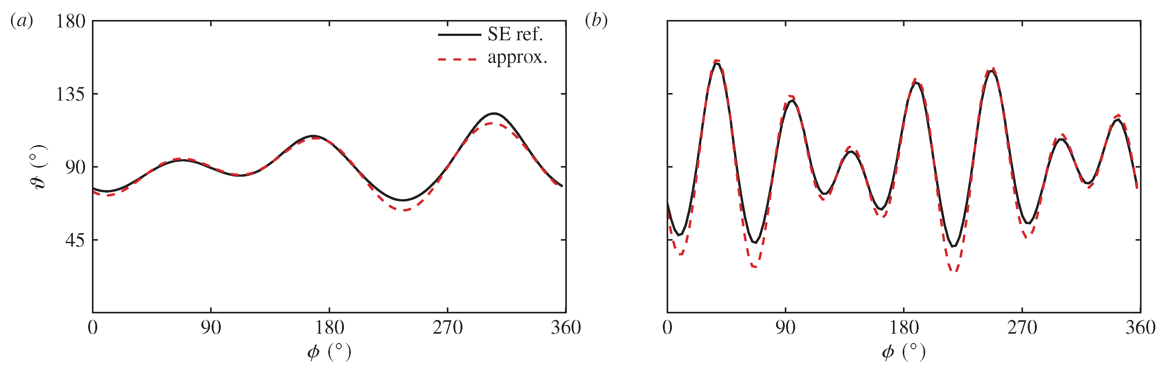
Figure A3.
Mean absolute and relative errors as a function of the wavenumber , for different amplitudes , considering droplets of dimensionless volume and contact line shapes of the form .
Figure A3.
Mean absolute and relative errors as a function of the wavenumber , for different amplitudes , considering droplets of dimensionless volume and contact line shapes of the form .
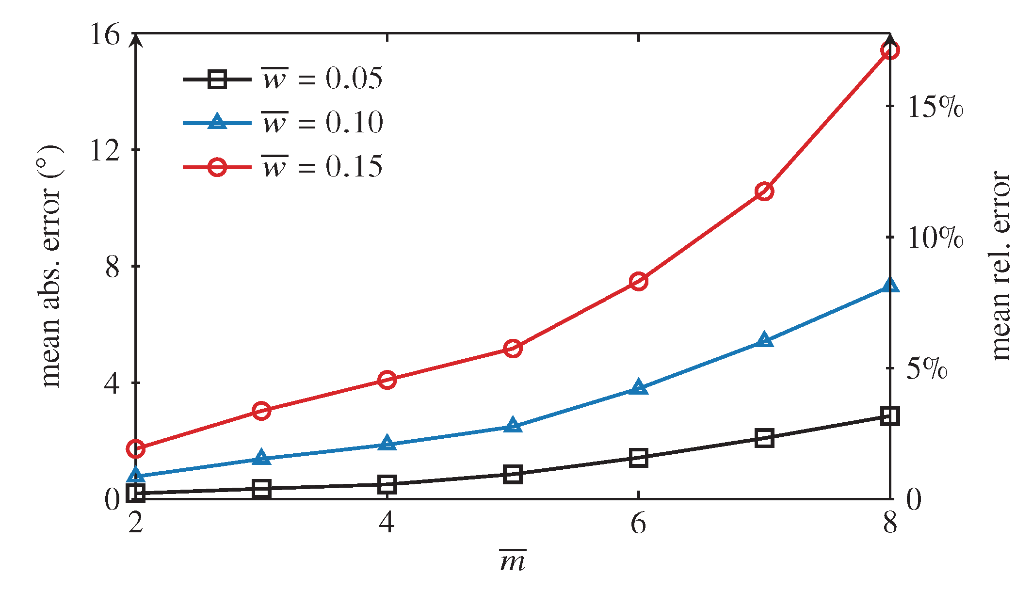
Figure A2 shows comparisons between the approximate contact angle calculated by Equation (A16) and reference solutions obtained using the surface evolver (SE) [60]. SE is a code that calculates the minimal energy surfaces in the presence of constraints and other physical effects such as gravity. It therefore provides an accurate estimation of the apparent contact angle, at a computational cost that is much larger compared to the approximate contact angle calculated by Equation (A16). Considering different contact line shapes of the form , the figure clearly shows that the approximation is not only affected by the amplitude of the perturbation ( and ), but also its wavenumber ( and ). This deviation is quantified in Figure A3, where the mean absolute error and mean relative error (considering a mean contact angle of ) are presented in terms of the perturbation amplitude and wavenumber, where and .
References
- Moragues, T.; Arguijo, D.; Beneyton, T.; Modavi, C.; Simutis, K.; Abate, A.R.; Baret, J.C.; deMello, A.J.; Densmore, D.; Griffiths, A.D. Droplet-based microfluidics. Nature Reviews Methods Primers 2023, 3, 32. [Google Scholar] [CrossRef]
- Zhang, Y.; Dong, Z.; Li, C.; Du, H.; Fang, N.X.; Wu, L.; Song, Y. Continuous 3D printing from one single droplet. Nature Communications 2020, 11, 4685. [Google Scholar] [CrossRef] [PubMed]
- Bonn, D.; Eggers, J.; Indekeu, J.; Meunier, J.; Rolley, E. Wetting and spreading. Reviews of Modern Physics 2009, 81, 739. [Google Scholar] [CrossRef]
- Wan, K.; Gou, X.; Guo, Z. Bio-inspired Fog Harvesting Materials: Basic Research and Bionic Potential Applications. Journal of Bionic Engineering 2021, 18, 501–533. [Google Scholar] [CrossRef]
- Podgorski, T.; Flesselles, J.M.; Limat, L. Corners, cusps, and pearls in running drops. Physical Review Letters 2001, 87, 036102. [Google Scholar] [CrossRef] [PubMed]
- Le Grand, N.; Daerr, A.; Limat, L. Shape and motion of drops sliding down an inclined plane. Journal of Fluid Mechanics 2005, 541, 293–315. [Google Scholar] [CrossRef]
- Miwa, M.; Nakajima, A.; Fujishima, A.; Hashimoto, K.; Watanabe, T. Effects of the surface roughness on sliding angles of water droplets on superhydrophobic surfaces. Langmuir 2000, 16, 5754–5760. [Google Scholar] [CrossRef]
- ElSherbini, A.I.; Jacobi, A.M. Critical contact angles for liquid drops on inclined surfaces. Surface and Colloid Science. Springer, 2004, pp. 57–62. [CrossRef]
- Morita, M.; Koga, T.; Otsuka, H.; Takahara, A. Macroscopic-wetting anisotropy on the line-patterned surface of fluoroalkylsilane monolayers. Langmuir 2005, 21, 911–918. [Google Scholar] [CrossRef] [PubMed]
- Berejnov, V.; Thorne, R.E. Effect of transient pinning on stability of drops sitting on an inclined plane. Physical Review E 2007, 75, 066308. [Google Scholar] [CrossRef]
- Suzuki, S.; Nakajima, A.; Tanaka, K.; Sakai, M.; Hashimoto, A.; Yoshida, N.; Kameshima, Y.; Okada, K. Sliding behavior of water droplets on line-patterned hydrophobic surfaces. Applied Surface Science 2008, 254, 1797–1805. [Google Scholar] [CrossRef]
- Bouteau, M.; Cantin, S.; Benhabib, F.; Perrot, F. Sliding behavior of liquid droplets on tilted Langmuir–Blodgett surfaces. Journal of Colloid and Interface Science 2008, 317, 247–254. [Google Scholar] [CrossRef] [PubMed]
- Varagnolo, S.; Schiocchet, V.; Ferraro, D.; Pierno, M.; Mistura, G.; Sbragaglia, M.; Gupta, A.; Amati, G. Tuning drop motion by chemical patterning of surfaces. Langmuir 2014, 30, 2401–2409. [Google Scholar] [CrossRef] [PubMed]
- Chaudhury, M.K.; Whitesides, G.M. How to make water run uphill. Science 1992, 256, 1539–1541. [Google Scholar] [CrossRef] [PubMed]
- Brunet, P.; Eggers, J.; Deegan, R. Vibration-induced climbing of drops. Physical Review Letters 2007, 99, 144501. [Google Scholar] [CrossRef]
- Savva, N.; Kalliadasis, S. Droplet motion on inclined heterogeneous substrates. Journal of Fluid Mechanics 2013, 725, 462–491. [Google Scholar] [CrossRef]
- Benilov, E.; Benilov, M. A thin drop sliding down an inclined plate. Journal of Fluid Mechanics 2015, 773, 75–102. [Google Scholar] [CrossRef]
- Thiele, U.; Velarde, M.G.; Neuffer, K.; Bestehorn, M.; Pomeau, Y. Sliding drops in the diffuse interface model coupled to hydrodynamics. Physical Review E 2001, 64, 061601. [Google Scholar] [CrossRef]
- Thiele, U.; Neuffer, K.; Bestehorn, M.; Pomeau, Y.; Velarde, M.G. Sliding drops on an inclined plane. Colloids and Surfaces A: Physicochemical and Engineering Aspects 2002, 206, 87–104. [Google Scholar] [CrossRef]
- Thiele, U.; Knobloch, E. Driven drops on heterogeneous substrates: Onset of sliding motion. Physical Review Letters 2006, 97, 204501. [Google Scholar] [CrossRef]
- Koh, Y.; Lee, Y.; Gaskell, P.; Jimack, P.; Thompson, H. Droplet migration: Quantitative comparisons with experiment. The European Physical Journal Special Topics 2009, 166, 117–120. [Google Scholar] [CrossRef]
- Afkhami, S.; Buongiorno, J.; Guion, A.; Popinet, S.; Saade, Y.; Scardovelli, R.; Zaleski, S. Transition in a numerical model of contact line dynamics and forced dewetting. Journal of Computational Physics 2018, 374, 1061–1093. [Google Scholar] [CrossRef]
- Cox, R. The dynamics of the spreading of liquids on a solid surface. Part 1. Viscous flow. Journal of Fluid Mechanics 1986, 168, 169–194. [Google Scholar] [CrossRef]
- Dimitrakopoulos, P.; Higdon, J. On the gravitational displacement of three-dimensional fluid droplets from inclined solid surfaces. Journal of Fluid Mechanics 1999, 395, 181–209. [Google Scholar] [CrossRef]
- Cavalli, A.; Musterd, M.; Mugele, F. Numerical investigation of dynamic effects for sliding drops on wetting defects. Physical Review E 2015, 91, 023013. [Google Scholar] [CrossRef]
- Fullana, T.; Zaleski, S.; Popinet, S. Dynamic wetting failure in curtain coating by the Volume-of-Fluid method: Volume-of-Fluid simulations on quadtree meshes. The European Physical Journal Special Topics 2020, 229, 1923–1934. [Google Scholar] [CrossRef]
- Sakakeeny, J.; Ling, Y. Numerical study of natural oscillations of supported drops with free and pinned contact lines. Physics of Fluids 2021, 33. [Google Scholar] [CrossRef]
- Han, T.Y.; Zhang, J.; Tan, H.; Ni, M.J. A consistent and parallelized height function based scheme for applying contact angle to 3D volume-of-fluid simulations. Journal of Computational Physics 2021, 433, 110190. [Google Scholar] [CrossRef]
- Dupuis, A.; Yeomans, J. Dynamics of sliding drops on superhydrophobic surfaces. Europhysics Letters 2006, 75, 105. [Google Scholar] [CrossRef]
- Varagnolo, S.; Ferraro, D.; Fantinel, P.; Pierno, M.; Mistura, G.; Amati, G.; Biferale, L.; Sbragaglia, M. Stick-slip sliding of water drops on chemically heterogeneous surfaces. Physical Review Letters 2013, 111, 066101. [Google Scholar] [CrossRef]
- Sbragaglia, M.; Biferale, L.; Amati, G.; Varagnolo, S.; Ferraro, D.; Mistura, G.; Pierno, M. Sliding drops across alternating hydrophobic and hydrophilic stripes. Physical Review E 2014, 89, 012406. [Google Scholar] [CrossRef]
- Borcia, R.; Borcia, I.D.; Bestehorn, M. Drops on an arbitrarily wetting substrate: A phase field description. Physical Review E 2008, 78, 066307. [Google Scholar] [CrossRef]
- Ramos, J.; Granato, E.; Ying, S.; Achim, C.; Elder, K.; Ala-Nissila, T. Dynamical transitions and sliding friction of the phase-field-crystal model with pinning. Physical Review E 2010, 81, 011121. [Google Scholar] [CrossRef]
- Do Hong, S.; Ha, M.Y.; Balachandar, S. Static and dynamic contact angles of water droplet on a solid surface using molecular dynamics simulation. Journal of colloid and interface science 2009, 339, 187–195. [Google Scholar] [CrossRef]
- Berim, G.O.; Ruckenstein, E. Microscopic calculation of the sticking force for nanodrops on an inclined surface. The Journal of chemical physics 2008, 129. [Google Scholar] [CrossRef] [PubMed]
- Das, A.K.; Das, P.K. Simulation of drop movement over an inclined surface using smoothed particle hydrodynamics. Langmuir 2009, 25, 11459–11466. [Google Scholar] [CrossRef] [PubMed]
- Brunton, S.L.; Noack, B.R.; Koumoutsakos, P. Machine learning for fluid mechanics. Annual Review of Fluid Mechanics 2020, 52, 477–508. [Google Scholar] [CrossRef]
- Sarghini, F.; De Felice, G.; Santini, S. Neural networks based subgrid scale modeling in large eddy simulations. Computers & Fluids 2003, 32, 97–108. [Google Scholar]
- Ling, J.; Kurzawski, A.; Templeton, J. Reynolds averaged turbulence modelling using deep neural networks with embedded invariance. Journal of Fluid Mechanics 2016, 807, 155–166. [Google Scholar] [CrossRef]
- Fukami, K.; Fukagata, K.; Taira, K. Super-resolution reconstruction of turbulent flows with machine learning. Journal of Fluid Mechanics 2019, 870, 106–120. [Google Scholar] [CrossRef]
- Fukami, K.; Fukagata, K.; Taira, K. Super-resolution analysis via machine learning: a survey for fluid flows. Theoretical and Computational Fluid Dynamics 2023, pp. 1–24. [CrossRef]
- Um, K.; Brand, R.; Fei, Y.R.; Holl, P.; Thuerey, N. Solver-in-the-loop: Learning from differentiable physics to interact with iterative pde-solvers. Advances in Neural Information Processing Systems 2020, 33, 6111–6122. [Google Scholar]
- Wan, Z.Y.; Sapsis, T.P. Machine learning the kinematics of spherical particles in fluid flows. Journal of Fluid Mechanics 2018, 857, R2. [Google Scholar] [CrossRef]
- Wan, Z.Y.; Karnakov, P.; Koumoutsakos, P.; Sapsis, T.P. Bubbles in turbulent flows: Data-driven, kinematic models with history terms. International Journal of Multiphase Flow 2020, 129, 103286. [Google Scholar] [CrossRef]
- Demou, A.D.; Savva, N. AI-assisted modeling of capillary-driven droplet dynamics. Data-Centric Engineering 2023, 4, e24. [Google Scholar] [CrossRef]
- Lacey, A. The motion with slip of a thin viscous droplet over a solid surface. Studies in Applied Mathematics 1982, 67, 217–230. [Google Scholar] [CrossRef]
- Savva, N.; Groves, D.; Kalliadasis, S. Droplet dynamics on chemically heterogeneous substrates. Journal of Fluid Mechanics 2019, 859, 321–361. [Google Scholar] [CrossRef]
- Tryggvason, G.; Scardovelli, R.; Zaleski, S. Direct numerical simulations of gas–liquid multiphase flows; Cambridge University Press, 2011.
- Popinet, S. Gerris: a tree-based adaptive solver for the incompressible Euler equations in complex geometries. Journal of Computational Physics 2003, 190, 572–600. [Google Scholar] [CrossRef]
- Popinet, S. An accurate adaptive solver for surface-tension-driven interfacial flows. Journal of Computational Physics 2009, 228, 5838–5866. [Google Scholar] [CrossRef]
- Popinet, S. A quadtree-adaptive multigrid solver for the Serre–Green–Naghdi equations. Journal of Computational Physics 2015, 302, 336–358. [Google Scholar] [CrossRef]
- Afkhami, S.; Bussmann, M. Height functions for applying contact angles to 2D VOF simulations. International Journal for Numerical Methods in Fluids 2008, 57, 453–472. [Google Scholar] [CrossRef]
- Afkhami, S.; Bussmann, M. Height functions for applying contact angles to 3D VOF simulations. International Journal for Numerical Methods in Fluids 2009, 61, 827–847. [Google Scholar] [CrossRef]
- Popinet, S. Numerical models of surface tension. Annual Review of Fluid Mechanics 2018, 50, 49–75. [Google Scholar] [CrossRef]
- Sakakeeny, J.; Ling, Y. Natural oscillations of a sessile drop on flat surfaces with mobile contact lines. Physical Review Fluids 2020, 5, 123604. [Google Scholar] [CrossRef]
- Negus, M.J.; Moore, M.R.; Oliver, J.M.; Cimpeanu, R. Droplet impact onto a spring-supported plate: analysis and simulations. Journal of Engineering Mathematics 2021, 128, 3. [Google Scholar] [CrossRef]
- Kovachki, N.; Li, Z.; Liu, B.; Azizzadenesheli, K.; Bhattacharya, K.; Stuart, A.; Anandkumar, A. Neural operator: Learning maps between function spaces. arXiv, 2021; arXiv:2108.08481. [Google Scholar]
- Li, Z.; Kovachki, N.; Azizzadenesheli, K.; Liu, B.; Bhattacharya, K.; Stuart, A.; Anandkumar, A. Fourier neural operator for parametric partial differential equations. arXiv, 2020; arXiv:2010.08895. [Google Scholar]
- Alt, H.; Godau, M. Computing the Fréchet distance between two polygonal curves. International Journal of Computational Geometry & Applications 1995, 5, 75–91. [Google Scholar]
- Brakke, K.A. The surface evolver. Experimental mathematics 1992, 1, 141–165. [Google Scholar] [CrossRef]
- Humplik, T.; Lee, J.; O’hern, S.; Fellman, B.; Baig, M.; Hassan, S.; Atieh, M.; Rahman, F.; Laoui, T.; Karnik, R.; et al. Nanostructured materials for water desalination. Nanotechnology 2011, 22, 292001. [Google Scholar] [CrossRef]
- Lee, A.; Moon, M.W.; Lim, H.; Kim, W.D.; Kim, H.Y. Water harvest via dewing. Langmuir 2012, 28, 10183–10191. [Google Scholar] [CrossRef]
- Sobac, B.; Brutin, D. Desiccation of a sessile drop of blood: Cracks, folds formation and delamination. Colloids and Surfaces A: Physicochemical and Engineering Aspects 2014, 448, 34–44. [Google Scholar] [CrossRef]
- Hartmann, S.; Diddens, C.; Jalaal, M.; Thiele, U. Sessile drop evaporation in a gap – crossover between diffusion-limited and phase transition-limited regime. Journal of Fluid Mechanics 2023, 960, A32. [Google Scholar] [CrossRef]
Figure 1.
Visualisation of a typical simulation setup, with an initially hemispherical droplet sitting on a chemically heterogeneous inclined surface. Darker shaded regions on the surface are more hydrophobic than lighter shaded regions.
Figure 1.
Visualisation of a typical simulation setup, with an initially hemispherical droplet sitting on a chemically heterogeneous inclined surface. Darker shaded regions on the surface are more hydrophobic than lighter shaded regions.
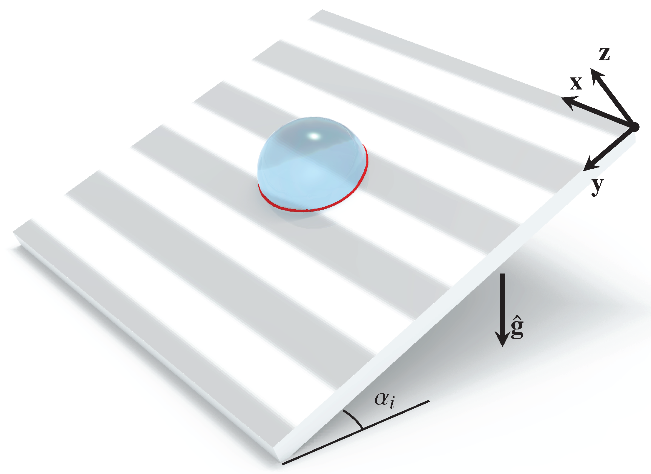
Figure 2.
Schematic representation of the FNO architecture as presented in [58]. Top panel: The overall architecture. First, operator lifts the input to a higher-dimensional space, followed by a series of Fourier layers, before operator projects the output back to the solution space. Bottom panel: Representation of a single Fourier layer. The input is passed through two parallel branches, before merging together to apply the activation function . In the top branch, forward and inverse Fourier transforms are applied to facilitate the learning of the weights in the Fourier space. In the bottom branch, a single local linear operator is applied.
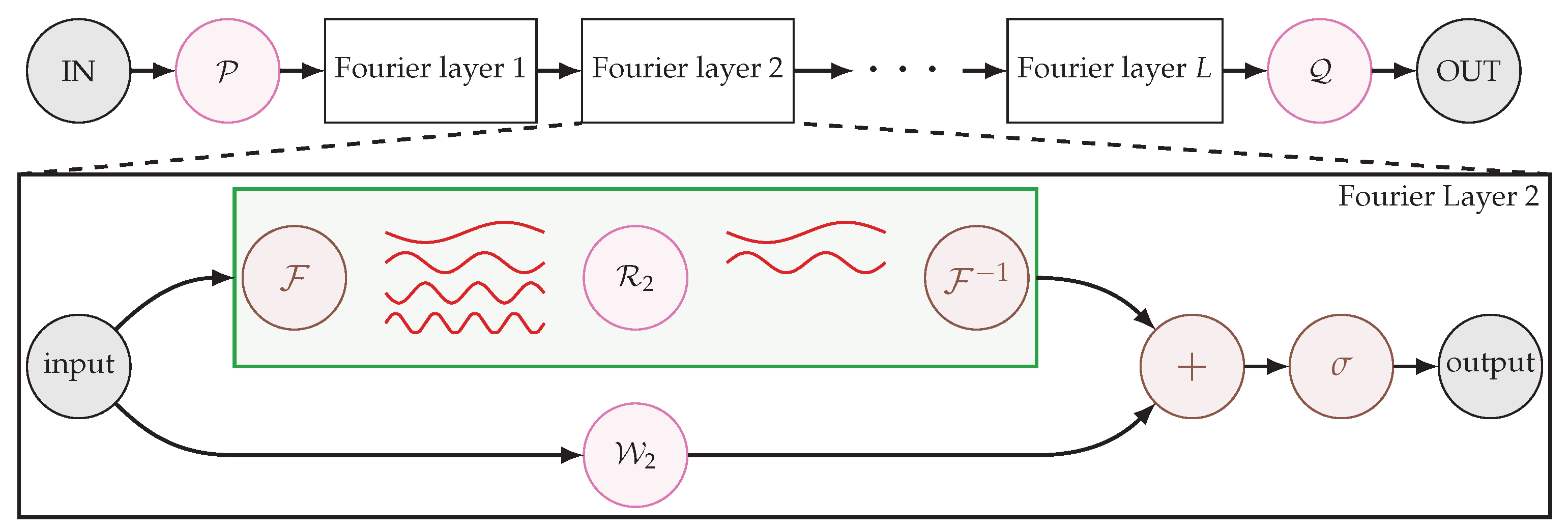
Figure 3.
Comparison between coarse simulations on an adaptive Cartesian grid with and (red dashed lines) and finer simulations with and (black lines), at different time instances. The errors based on the Fréchet distance are 2.4% at and 4.8% at . The background shading describes the heterogeneity profile on the substrate.

Figure 4.
Training and testing errors as a function of the number of epochs. Two different sample sizes are considered, with (red lines; and ) and (black lines; and ). Dashed and solid curves show the training errors and testing errors , respectively.
Figure 4.
Training and testing errors as a function of the number of epochs. Two different sample sizes are considered, with (red lines; and ) and (black lines; and ). Dashed and solid curves show the training errors and testing errors , respectively.
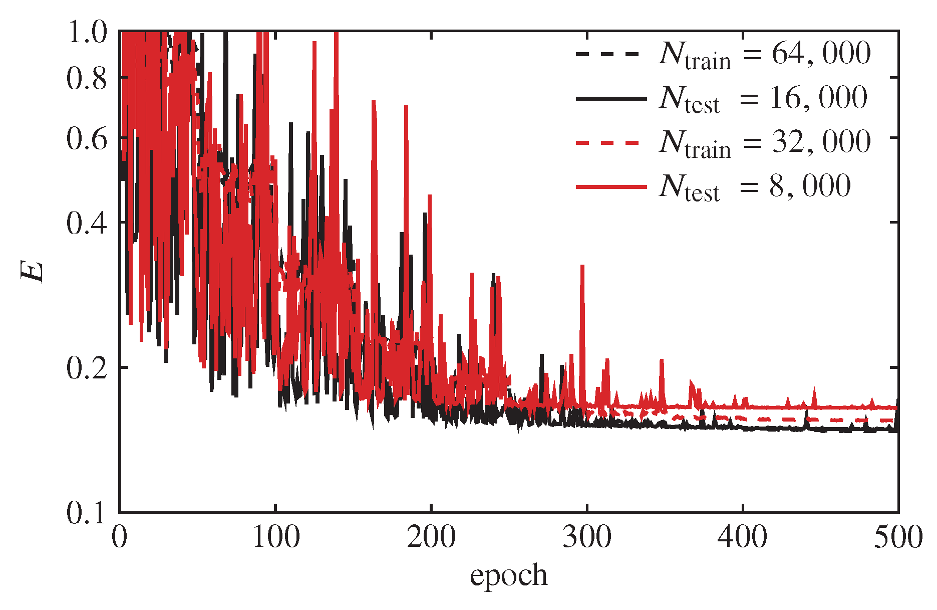
Figure 5.
Azimuthal distribution of different velocity components under (a) Bo=5 and , and (b) Bo=5 and . The trajectory followed by the droplet and the heterogeneity profile used in these cases are depicted in Figure 8(a) and (c) respectively. The distributions presented in this figure correspond to . The predicted solution (red line) is calculated by summing the reduced order model prediction (blue line) and the AI model prediction (red dashed line).
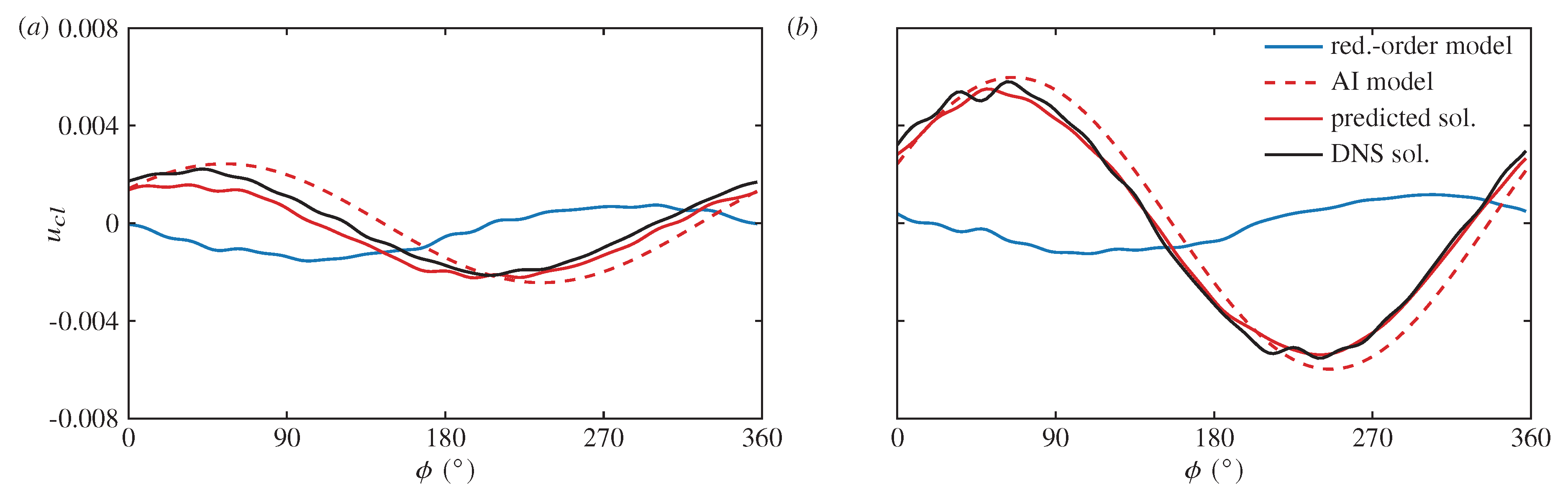

Table 1.
Test errors for the different FNO-related hyper-parameters, namely the width w of the channel space after the application of the lifting operator , and the number of Fourier layers (see Figure 2). The lowest testing error is highlighted with gray background.
Table 1.
Test errors for the different FNO-related hyper-parameters, namely the width w of the channel space after the application of the lifting operator , and the number of Fourier layers (see Figure 2). The lowest testing error is highlighted with gray background.
| w | ||||
|---|---|---|---|---|
| 32 | 0.203 | 0.183 | 0.164 | 0.153 |
| 64 | 0.203 | 0.182 | 0.165 | 0.149 |
| 128 | 0.204 | 0.174 | 0.164 | 0.151 |
| 256 | 0.205 | 0.169 | 0.163 | 0.152 |
Disclaimer/Publisher’s Note: The statements, opinions and data contained in all publications are solely those of the individual author(s) and contributor(s) and not of MDPI and/or the editor(s). MDPI and/or the editor(s) disclaim responsibility for any injury to people or property resulting from any ideas, methods, instructions or products referred to in the content. |
© 2024 by the authors. Licensee MDPI, Basel, Switzerland. This article is an open access article distributed under the terms and conditions of the Creative Commons Attribution (CC BY) license (http://creativecommons.org/licenses/by/4.0/).
Copyright: This open access article is published under a Creative Commons CC BY 4.0 license, which permit the free download, distribution, and reuse, provided that the author and preprint are cited in any reuse.


