
Submitted:
12 March 2024
Posted:
13 March 2024
You are already at the latest version
Abstract
High-resolution wave measurements at intermediate water depth are required to improve coastal impact modeling. Specifically, such data sets are desired to calibrate and validate models, and broaden the insight on the boundary conditions that force models. Here, we present a wave data set collected in the North Sea at three stations in intermediate water depth (6-14~m) during the 2021/2022 storm season as part of the RealDune/REFLEX experiments. Continuous measurements of synchronized surface elevation, velocity and pressure were recorded at 2-4~Hz by Acoustic Doppler Profilers and an Acoustic Doppler Velocimeter for a 5~month duration. Time series were quality-controlled, directional-frequency energy spectra were calculated, and common bulk parameters were derived. Measured wave conditions vary from calm to energetic with 0.1-5.0~m sea-swell wave height, 5-16~s mean wave period and W-NNW direction. Nine storms, i.e. wave height beyond 2.5~m for at least six hours, were recorded including the triple storms Dudley, Eunice and Franklin. This unique data set can be used to investigate wave transformation, wave nonlinearity and wave directionality for higher and lower frequencies (e.g. sea-swell and infragravity waves) to compare with theoretical and empirical descriptions. Furthermore, the data can serve to force, calibrate and validate models during storm conditions.
Keywords:
Wave measurements
; velocity measurements
; wave transformation
; ADCP
; ADV
1. Summary
Waves are a known hazard along coastlines, as they can cause failure of coastal defense structures but also dune erosion and barrier island breaching [1,2] that can ultimately lead to marine flooding of the low-lying hinterland. The waves that dominate the coastal zone are sea-swell (SS) and infragravity (IG) waves, with wave periods between 3-25 s and 25-250 s, respectively. During storms, SS and IG wave energy increases. Once SS waves reach shallow water, a large part of their energy is dissipated by wave breaking. In contrast, IG waves experience limited dissipation when propagating onshore, and increasingly dominate the water motion. During storms, IG waves have been observed to reach wave heights up to 1 m or more in shallow water [3,4,5,6].
Process-based numerical models are used to predict the transformation of the SS and IG wave field from offshore to shallow waters under extreme conditions including future scenarios to assess coastal safety. However, uncertainties remain regarding the required formulation of the offshore boundary conditions typically located in intermediate water depth during these storm conditions. Due to lack of information on the true boundary conditions, these models are often forced with boundary conditions that are reconstructed from reduced input (e.g., bulk wave statistics), assuming a certain frequency and directional spectral shape, randomly distributed wave phase and ignoring or parameterizing IG energy that is not locally generated (e.g., [7,8,9]). Consequently, nearshore wave predictions contain uncertainty [8,10], especially during extreme conditions. These nearshore predictions of process-based numerical models can be improved by model calibration and validation, and by a more accurate definition of the offshore boundary conditions. Hereto, data are required.
High resolution data from offshore to onshore have been acquired in laboratories, but data sets are generally biased to simplified experimental designs that are not always representative of field conditions (e.g., alongshore uniform bathymetry, shore-normal wave incidence, unimodal wave field). Instead, field data sets have allowed the investigation of wave dynamics in various settings (e.g., oceans, regional seas, open coasts, barrier islands, reef-lined coasts) with different wave climates (storms, hurricanes, sea breeze). Fixed measurement stations such as buoy networks provide long-term frequency-directional wave data at various locations, usually tens of kilometers offshore and in large water depth (>20 m). In addition, dedicated field campaigns acquire frequency-directional wave data typically from an array of instruments deployed for a period of days-weeks in smaller water depths (<5 m), where instruments are relatively easy to deploy, survey and recollect. However, data that aid improving our insights on the model boundary conditions for both regional-scale models and local-scale coastal models need to be collected in intermediate water depths along a cross-shore array and, moreover, contain information on the SS and IG directional field. Only a few frequency-directional data sets have been gathered in such water depths (e.g., [11,12,13]), often with a limited number of stations or in relatively shallow depths.
Here, we present a high-resolution, 5-month data set collected in intermediate water depth (6-14 m) in the North Sea during the storm season of November 2021 to April 2022. Three bottom frames were deployed with Acoustic Doppler Current Profilers (ADCPs) and an Acoustic Doppler Velocity meter (ADV) to measure pressure, water depth, velocity and temperature continuously at 2 or 4 Hz. Sea surface elevation was accurately measured through acoustic surface tracking (AST) by the built-in altimeter on the ADCPs, allowing to record short waves at larger water depths to fully resolve the SS wave conditions. The data set was collected during the RealDune/REFLEX field experiments, which were initiated to reduce uncertainty in dune safety predictions. Two artificial dunes were constructed close to the high water line to ensure dune attack events. Subsequently, instruments were deployed in the intertidal and subtidal zone. The 6-week duration intertidal and neardune hydro- and morphodynamic data set are presented in Van Wiechen et al. [14], whereas the subtidal data set of 5-month duration is described in this contribution. The subtidal experimental design was primarily aimed at investigating the spatiotemporal variability of the directional characteristics of the IG wave field along the Dutch coast to improve the definition of the offshore boundary conditions in dune safety assessments. The data set can be used more widely to investigate wave transformation, SS and IG wave directionality and wave nonlinearity to compare with theoretical and empirical descriptions, but can also serve to force and validate numerical models.
2. Study Site
The data set was collected in the southern North Sea near the Sandmotor mega-nourishment, The Netherlands (Figure 1). The regional coastline is roughly southwest-northeast oriented (40 deg N). The profile is characterized by a foreshore slope of 1:115 (between -3.5 m and 0 m with respect to Mean Sea Level (MSL)), one or two subtidal bars of ∼1 m, and a lower shoreface slope of 1:483 (between -10 m and -4 m MSL; Figure 2). The profile is rather flat offshore due to dumped dredged sediments from Rotterdam harbour.
The site is exposed to a bimodal wave climate with waves mainly coming from the southwest and north-northwest and a yearly-averaged significant wave height, , of 1.2 m and peak wave period, , of 6 s. The autumn-winter season (October - April) is characterized by storms with up to 6 m, of 10 s and elevated water levels of up to 3 m. Storm surge is especially high during northwestern storms. The tide is semidiurnal with a spring tidal range of 2.2 m and a neap tidal range of 1.3 m. Flood and ebb currents are upcoast and downcoast directed and reach velocities of 0.7 m/s in a water depth of ∼7 m.
3. Instrumentation and Data Collection
The data set ranges from 15 November 2021 7:00 UTC to 13 April 2022 11:00 UTC, and was collected at three frames positioned on the sea floor in a cross-shore array that aligned with the instrument array in the intertidal zone described in [14] (Figure 2). Hereafter, the three frames are referred to as F1, F2 and F3 (Table 1). F1 and F2 were both deployed with a Nortek Signature 1000 ADCP (Figure 3a-b). Both frames also contained a Teleydyne RDI Workhorse ADCP (600kHz at F1 and 1200 kHz at F2). Note that the Signature ADCPs were aimed to serve as the primary source of data and that the Workhorse ADCPs at F1 and F2 were installed for redundancy. F3 was equipped with a flexible head Nortek Vector ADV (15 Nov - 24 Jan) and a Teledyne RDI Workhorse 1200kHz (24 Jan - 13 Apr; Figure 3c-d). All ADCPs were installed upward-looking, whereas the ADV probe was deployed horizontally. The frames were surveyed once during the five-month campaign on 24 January 2022 to replace batteries, read out data, and switch instruments. The first and second measurement periods are hereafter referred to as P1 (15 Nov 2021 - 24 Jan 2022) and P2 (24 Jan - 13 Apr 2022), respectively.
The Signature ADCPs sampled continuously at 4 Hz, collecting pressure, distance from sensor to the water surface, and velocities over the full water column. Distance to the water surface was measured through acoustic surface tracking with the vertical beam. Blanking distance, cell size, and cell number differed between F1 and F2. In addition, a 2-min average flow profile was sampled every hour. For the specific settings see Table 2. The Workhorse ADCPs were programmed to have a similar sampling scheme as the Signature ADCPs, as far as allowed by the available memory space and battery power. This resulted in sampling every two hours for one hour at 2 Hz, collecting pressure, water depth, and velocities in five cells spread over the water column. The Workhorse ADCPs did not have a vertical beam to measure the distance to the water surface, but instead provided the distance from the sensor to the water surface along the four slanted beams. An average flow profile was sampled every 2 minutes. Blanking distance, cell size, and cell number differed between the frames, see Table 3. The Vector ADV sampled the pressure and velocities at a single depth close to the bottom continuously at 4 Hz. For configuration settings see Table 4. Before deployment, the clocks of all instruments were synchronized with the computer clock that was synchronized with https://time.is.
All frames were successfully deployed on the bottom and had a minor tilt angle throughout the campaign (<9 deg), except for F2 during period P1 (F2P1 in the following). The Signature ADCP on this frame had a pitch of -7 deg and roll of 3 deg after deployment, whereof the pitch changed to -14 deg during the first substantial storm (1 December 2021), requiring corrections on the data before usage. All instruments functioned and collected data for most of the campaign. For an overview of data collection periods see Figure 2. Some of the Workhorse ADCPs ran out of battery and stopped measuring before the instruments were retrieved. The velocity probe of the ADV at F3 rotated (Figure 4a-b). The moment of damage was identified on 21 December 2021 07:00, coinciding with a 5-min disturbance in the heading signal and a change in the velocity signal that persisted for the rest of the campaign (Figure 4c-e). As a consequence, the velocity data after 21 December required correction before usage (Section 5.1).
Heading measurements can be inaccurate due to magnetic declination (i.e., the deviation of magnetic north from true north) and due to a deviation related to the influence of metals objects on the compass measurement. A compass validation procedure was carried out after the campaign to assess the importance of compass deviations due to the frame and/or battery canisters. Hereto, the frames with ADCPs were positioned outside of the laboratory as far away as possible from other metal objects that could influence the compass. ADCP-measured heading was compared to the orientation of the ADCP measured with a differential GPS. Differences were small (1-2 degrees) for the ADCPs that were validated and therefore we decided to not correct ADCP-measured heading in post-processing.
Clock drift was determined after recollection of the instruments. The Signature ADCP clocks were slightly behind (F1P1: -5s, F1P2: -5 s, F2P1: -5 s, F2P2: -3 s), the ADV clock 10 s ahead, whereas the Workhorse ADCP clocks drifted most (F1P2: -6 s, F2P2: +267 s, F3P2: - 43 s; no clock drift determined for P1). Data were not corrected for clock drift.
4. Data Description
The data set is publicly available from the 4TU data center https://data.4tu.nl/collections/233f11ff-7804-4777-8b32-92c4606e56d8. Data are organized in folders per frame, with each folder containing a raw data file and a netcdf file with variables extracted from the raw data file. Also, processed data are provided, including hourly frequency-direction spectra and bulk statistics. Furthermore, a folder with supplementary data is provided.
4.1. ADCP and ADV data
Variables collected by the Signature 1000 ADCPs include vertical distance from the sensor to the surface, water pressure, temperature, sensor orientations (i.e., pitch, roll, and heading), and velocity in depth cells over the full water column. For a complete list see Table 5. Variables collected by the Workhorse ADCPs contain water pressure, distance from the sensor to the surface along the slanted beams, temperature, sensor orientations and velocity in five depth cells spread over the water column (see Table 6). The positions of the depth cells are located near the sensor (cell 1), halfway the water column (cell 2) and close to the water surface (cell 3-5), and vary over time with the mean water depth. Variables collected by the Vector ADV include water pressure, velocity at a single depth, temperature and sensor orientations (see Table 7).
4.2. Supplementary Data
Supplementary data include measurements of air pressure, water levels and bed elevation, which are stored in the folder supplementaryData. Air pressure data, , from the closest meteorologic station (Hoek van Holland) were downloaded from https://www.knmi.nl/nederland-nu/klimatologie/uurgegevens/. Tidal elevation at the study site was obtained as the weighted average of the signal at the two closest tidal stations (Scheveningen and Hoek van Holland; https://waterinfo.rws.nl) and stored in a netcdf file. Bed elevation, was measured from -12 m to +5.5 m MSL just before data collection started (3 November 2021) and a few weeks after (17 December 2021). Cross-shore bed elevation profiles along the frame locations were extracted from these data and stored in a netcdf file. The profile data are available in the RD coordinate system, and along a local system with the x-axis directed along the frames (295 deg) pointing seaward and the origin just behind the crest of the artificial dune (= 72400 m, =451865 m).
4.3. Processed Data
Processed data include hourly estimates of frequency-direction surface elevation spectra and corresponding bulk parameters at the three frames for the 5-month study period. Data from the Signature ADCP were used for F1 and F2, whereas data from the Vector ADV (Nov-Jan) and Workhorse ADCP (Jan-Apr) were used for F3. Bulk parameters include SS and IG significant wave height ( and ), mean wave period ( and ), peak wave period (), SS wave direction (), and mean water depth ().
5. Methods
5.1. Initial Data Processing
The Signature ADCP data were read from the instruments through an Ethernet connection. The raw data files (.ad2cp format) were converted to readable files (.mat) of 1-day duration using the freely-available Signature Deployment software (Nortek). At the same time, the software calculated the coordinate transformation from beam coordinates to East-North-Up (ENU) coordinates of the velocity data and included these in the converted .mat files, used for further processing. The Workhorse ADCP data were read from the instruments through a serial port. Raw data files (.000) were converted to readable format (.txt) with Pkts2Txt.exe for each deployment. Heading, pitch, and roll data were extracted using ViSea DPS (Aquavision B.V.) as .csv format. ADV data were read directly from the SD card, obtaining several files in readable format (.dat, .hdr, .sen, .pck, .ssl, .vec, .vhd).
Several processing steps were carried out to obtain netcdf files for all instruments:
- Construction of time series of 5-month duration for the variables of interest from each instrument with equidistant time interval (1-4 Hz depending on the variable and the instrument);
- Pressure correction for atmospheric pressure and pressure offset of the instrument. Pressure offsets () were determined when the instrument was out of the water just before and after deployment;
- Matrix rotation to obtain velocities in ENU coordinate system from beam coordinate system (Workhorse ADCPs) and xyz coordinate system (ADV). A 6-min average was used for heading, pitch and roll in the matrix rotations. For the Signature ADCPs, coordinate transformation was performed using the deployment software. Note that heading and ENU velocities were corrected for the magnetic declination at the moment of the campaign (+1.87 deg East);
- Depth cell mapping on the velocity data for F2P1 to correct for the large tilt angle using the Ocean Contour software of Ocean Illumination;
- Additional matrix rotation to roughly correct for the bent ADV fork. Hereto, the heading and pitch were corrected by 23 and 20 degrees for the data collected after 21 December 2021 7:00am, with corrections following from angle measurements of the bent fork on the frame;
- Storage of time series of interest in netcdf files.
5.2. Data quality
5.2.1. Signature ADCPs
Variables in Table 5 contain some data that were recorded when the instrument was out of the water (0.4% for both F1 and F2). Those data points were identified, stored in a new variable (; Table 5) and added to the netcdf file.
Inspection of the acoustic surface tracking signal () showed the need for quality control. Intermittently, dropped unrealistically by a few meters for seconds to minutes (Figure 5a), which contaminated the low-frequency signal. The drop in the water level was observed more frequently during storms, although it was not limited to such conditions. Possibly, the water level drop was related to the reflection of the altimeter signal on bubbles just below the surface caused by wave breaking. A two-step quality control routine was designed to prepare the data for further analysis. Poor quality data were identified and flagged (). First, bursts with water level drops were identified by calculating the standard deviation, , per 1-hr burst
where and are the quadratically detrended and lowpass-filtered (f<0.01 Hz) AST-derived and pressure-derived water depths, respectively. is higher for bursts that contain the water level drop in . An adequate threshold of to flag bursts was determined by evaluating the percentage of flagged bursts as a function of . We adopted >0.2 m as threshold, flagging 20 1-hr bursts (0.6% of the data) for F1, and 59 1-hr bursts (1.7% of the data) for F2. Second, data points were flagged if spikes were detected with the phase-space despiking method of [15,16] on 1-hr bursts of quadratically detrended (Figure 5b). Herein, the universal threshold (Equation 2 in [15]) was multiplied by 1.25 to prevent identifying high, skewed waves as spikes. This resulted in flagging 0.04% of the data for F1 and 0.10% of the data for F2. Flagged data were stored in (Table 5), which was added to the netcdf file.
In addition, inspection of the velocity signals revealed the need for quality control as spikes appeared at a semi-regular interval at both F1 and F2 (Figure 6a). First, data were flagged if <50% (following [17]) for at least one of the beams. Cells closer to the surface were flagged more often as decreased with distance from the sensor (Figure 7a). This resulted in flagging up to 12% for both F1 and F2 close to the water surface (14 m and 8 m from the bottom respectively). Second, data were flagged if spikes were detected in one of the beams, resulting in flagging an additional 0.7% of the data for F1 at 13 m from the bottom and 0.5% for F2 at 8 m from the bottom (Figure 6b, Figure 7c-d). Flagged data were stored in (Table 5), which was added to the netcdf file. Note that we created only a single for all four beams, with the reasoning that poor quality data in even a single beam can translate into poor quality analysis outcomes when using all four beams as input.
5.2.2. Workhorse ADCPs
Data from F1 and F2 contain NaNs at the end of the time series because the ADCPs ran out of battery. Velocity data at F2 contain NaNs throughout the time series. For F3P2, 65% of the velocity time series contains NaNs because velocity stopped being recorded.
Poor quality data points were identified when the instrument was out of the water (; Table 6). In the velocity data, additional poor quality data points were identified by despiking (). In the first cell, 0.02% of the data were flagged due to spikes at F1 (3-9 m from the bottom), 0.16% at F2 (2 m from the bottom), and 0.02% at F3 (2 m from the bottom). Additional quality control based on correlation values was not possible because this information was not available for the Workhorse ADCPs. Gaps throughout the time series at F2 resulted in extra detection of spikes, because data points around the gaps were often detected as spikes. Possibly, a technical problem existed during data recording at this frame as the data recorded at F1 and F3 contained significantly fewer gaps.
5.2.3. Vector ADV
Poor quality data points were identified when the instrument was out of the water (1.7% of the data; ; Table 7). Poor quality velocity data were identified from low signal-to-noise ratios and correlation values, using the same thresholds as [18]. In addition, spikes were identified in the velocity data. All identified poor quality data points were stored in (0.3% of the data) and added to the netcdf file.
5.3. Processed Parameters
Frequency-direction surface elevation spectra () were calculated with the Maximum Entropy Method [19] per 1-hr burst, using , and as input. Hereto, and were used that were measured 10.2 m (F1), 6.0 m (F2) and 2.0 m (F3) from the bottom. Additional frequency-directional surface elevation spectra () were calculated for F1 and F2 using instead of . First, time series were flagged using , and . Gaps related to and were linearly interpolated if they were smaller than 1 s and filled with a 1 s-moving average of the raw data if they were larger than 1 s. Then, spectra were calculated by dividing quadratically detrended 1-hr time series into blocks of 256 s, using 50% overlap and tapering each block with a Hamming window. This resulted in 68 effective degrees of freedom. To obtain , a transfer function based on linear wave theory was applied to convert the pressure spectrum into an elevation spectrum.
Subsequently, bulk parameters were obtained for each 1hr-burst by integrating the frequency-direction spectra over direction, bandpass filtering on SS (0.04-0.33 Hz) and IG (0.004-0.04 Hz) frequencies, and calculating the respective 0, 1st and 2nd order spectral moments (, , ). SS wave parameters were calculated from , which is based on direct measurements of the sea-surface () and thus captured better energy in high frequencies than . Instead, IG wave parameters were calculated from , because the low frequency part of was found sensitive to the observed water level drops in (Figure 5a, see also Section 6). Significant wave heights were estimated as and , whereas mean wave periods were calculated as and . Peak SS wave period () and peak SS wave direction () were calculated from the respective peaks in the direction-integrated and frequency-integrated spectra.
6. Usage Notes
The water level drop in contaminates energy at low frequencies, such as the IG-band. Therefore, we recommend to use instead for low-frequency analysis. In contrast, we recommend to use when interested in higher frequencies (e.g., SS-band) as shorter waves are well captured in the signal and analysis is not affected by the water level drop.
Data were quality-controlled following commonly-applied filtering routines. Data points identified as low quality can be identified using the provided flag vectors (Table 5, Table 6 and Table 7). It was chosen to provide the raw time series together with these flag vectors rather than corrected time series because the best approach to deal with these low quality points depends on the intended analysis. It should furthermore be noted that the despiking method was not always able to identify all spikes if many were present. Depending on intended usage, bursts containing a high number of flagged data points may be better entirely discarded.
Figure 8 shows an overview of the hydrodynamic conditions during the study period. Wave roses (Figure 9) indicate how the two dominant directional modes during the study period changed from north and southwest at the Europlatform (32 m depth, see Figure 1) to northwest and west at the most onshore location (F3). Several storms passed during the study period, whereof statistics are given in Table 8. Here, storms are defined as periods of at least 6 hr with 2.5 m. Statistics in Table 8 correspond to maximum values during the storm except for , which is the energy-weighted mean angle during the storm. The artificially constructed dunes experienced erosion during storm 1, storm 2, storm 3 and storm 4. The dune that was constructed in line with the transect through F1, F2, and F3 persisted until storm 4, whereas the dune that was constructed 500 m upcoast persisted until storm 2. See [14] for an extensive description of the dune development and the data collected in the nearshore.
Author Contributions
Conceptualization, J.R., M.T., and A.R.; methodology, J.R., M.T., A.R., X.Z., P.W. and S.V.; software, J.R., X.Z., and A.R. validation, J.R.; formal analysis, J.R., X.Z.; investigation, J.R., X.Z., M.T., P.W. and J.W.M.; resources, M.T. and J.W.M.; data curation, J.R.; writing—original draft preparation, J.R.; writing—review and editing, J.R., M.T., A.R., P.W., S.V., X.Z. and J.W.M.; visualization, J.R., P.W., and M.T.; supervision, M.T.; project administration, M.T.; funding acquisition, M.T., A.R., and S.V. All authors have read and agreed to the published version of the manuscript.
Funding
This research was part of the REFLEX and Realdune projects funded by TKI Deltatechnologie (project codes TU04 and TU06).
Data Availability Statement
Data described in this manuscript is available from 4TU data center (https://data.4tu.nl/collections/233f11ff-7804-4777-8b32-92c4606e56d8).
Acknowledgments
We acknowledge technical support by Pieter van der Gaag, Arie van der Vlies, Arno Doorn, and Chantal Willems from the Hydraulic Engineering laboratory as well as the support from DEMO at Delft University of Technology. In addition, we acknowledge support on ADCP programming and data retrieval by Jorg Eij from Aquavision B.V., Loic Michel from Teledyne France and Rikke van der Grinten from Nortek. We thank Dannie Beks and Anke Cotteleer from Rijkswaterstaat for preparing the frames for deployment and data retrieval from the Workhorses. In addition, we acknowledge France Floc’h for guidance during the processing of the Workhorse data. Furthermore, we thank Arjen Ponger and the crew of the Rijkswaterstaat vessel for the deployment of the measurement frames.
Conflicts of Interest
The authors declare no conflict of interest. The funders had no role in the design of the study; in the collection, analyses, or interpretation of data; in the writing of the manuscript; or in the decision to publish the results.
References
- Thornton, E.B.; MacMahan, J.; Sallenger, A., Jr. Rip currents, mega-cusps, and eroding dunes. Marine Geology 2007, 240, 151–167. [Google Scholar] [CrossRef]
- Roelvink, D.; Reniers, A.; Van Dongeren, A.; De Vries, J.V.T.; McCall, R.; Lescinski, J. Modelling storm impacts on beaches, dunes and barrier islands. Coastal Engineering 2009, 56, 1133–1152. [Google Scholar] [CrossRef]
- Guza, R.T.; Thornton, E.B. Swash oscillations on a natural beach. Journal of Geophysical Research: Oceans 1982, 87, 483–491. [Google Scholar] [CrossRef]
- Ruessink, B.; Kleinhans, M.; Van den Beukel, P. Observations of swash under highly dissipative conditions. Journal of Geophysical Research: Oceans 1998, 103, 3111–3118. [Google Scholar] [CrossRef]
- Inch, K.; Davidson, M.; Masselink, G.; Russell, P. Observations of nearshore infragravity wave dynamics under high energy swell and wind-wave conditions. Continental Shelf Research 2017, 138, 19–31. [Google Scholar] [CrossRef]
- Bertin, X.; Martins, K.; de Bakker, A.; Chataigner, T.; Guérin, T.; Coulombier, T.; de Viron, O. Energy Transfers and Reflection of Infragravity Waves at a Dissipative Beach Under Storm Waves. Journal of Geophysical Research: Oceans 2020, 125, e2019JC015714. [Google Scholar] [CrossRef]
- Almeida, L.P.; Masselink, G.; McCall, R.; Russell, P. Storm overwash of a gravel barrier: Field measurements and XBeach-G modelling. Coastal Engineering 2017, 120, 22–35. [Google Scholar] [CrossRef]
- Fiedler, J.W.; Smit, P.B.; Brodie, K.L.; McNinch, J.; Guza, R. The offshore boundary condition in surf zone modeling. Coastal Engineering 2019, 143, 12–20. [Google Scholar] [CrossRef]
- Rijnsdorp, D.P.; Reniers, A.J.H.M.; Zijlema, M. Free Infragravity Waves in the North Sea. Journal of Geophysical Research: Oceans 2021, 126, e2021JC017368. [Google Scholar] [CrossRef]
- Rutten, J.; Torres-Freyermuth, A.; Puleo, J. Uncertainty in runup predictions on natural beaches using XBeach nonhydrostatic. Coastal Engineering 2021, 166, 103869. [Google Scholar] [CrossRef]
- Herbers, T.; Elgar, S.; Guza, R. Infragravity-frequency (0.005–0.05 Hz) motions on the shelf. Part I: Forced waves. Journal of Physical Oceanography 1994, 24, 917–927. [Google Scholar] [CrossRef]
- Fiedler, J.W.; Brodie, K.L.; McNinch, J.E.; Guza, R.T. Observations of runup and energy flux on a low-slope beach with high-energy, long-period ocean swell. Geophysical Research Letters 2015, 42, 9933–9941. [Google Scholar] [CrossRef]
- Van Prooijen, B.C.; Tissier, M.F.; De Wit, F.P.; Pearson, S.G.; Brakenhoff, L.B.; Van Maarseveen, M.C.; Van Der Vegt, M.; Mol, J.W.; Kok, F.; Holzhauer, H.; et al. Measurements of hydrodynamics, sediment, morphology and benthos on Ameland ebb-tidal delta and lower shoreface. Earth System Science Data Discussions 2020, 2020, 1–18. [Google Scholar] [CrossRef]
- Van Wiechen, P.; Rutten, J.; De Vries, S.; Tissier, M.; Mieras, R.; Anarde, K.; Baker, C.; Reniers, A.; Mol, J. Measurements of dune erosion processes during the RealDune/REFLEX experiments. Scientific Data 2024(accepted).
- Goring, D.G.; Nikora, V.I. Despiking acoustic Doppler velocimeter data. Journal of Hydraulic Engineering 2002, 128, 117–126. [Google Scholar] [CrossRef]
- Mori, N.; Suzuki, T.; Kakuno, S. Noise of acoustic Doppler velocimeter data in bubbly flows. Journal of Engineering Mechanics 2007, 133, 122–125. [Google Scholar] [CrossRef]
- Nortek. Principles of Operation - Signature, 2022.4 ed., 2022.
- Elgar, S.; Raubenheimer, B.; Guza, R. Quality control of acoustic Doppler velocimeter data in the surfzone. Measurement Science and Technology 2005, 16, 1889. [Google Scholar] [CrossRef]
- Lygre, A.; Krogstad, H.E. Maximum entropy estimation of the directional distribution in ocean wave spectra. Journal of Physical Oceanography 1986, 16, 2052–2060. [Google Scholar] [CrossRef]
Figure 1.
Location of study site with the three frames F1-F3 during the RealDune/REFLEX experiments and the position of the Europlatform (EUR) wave station in the Dutch coordinate system (RD; Rijksdriehoekstelsel).
Figure 1.
Location of study site with the three frames F1-F3 during the RealDune/REFLEX experiments and the position of the Europlatform (EUR) wave station in the Dutch coordinate system (RD; Rijksdriehoekstelsel).
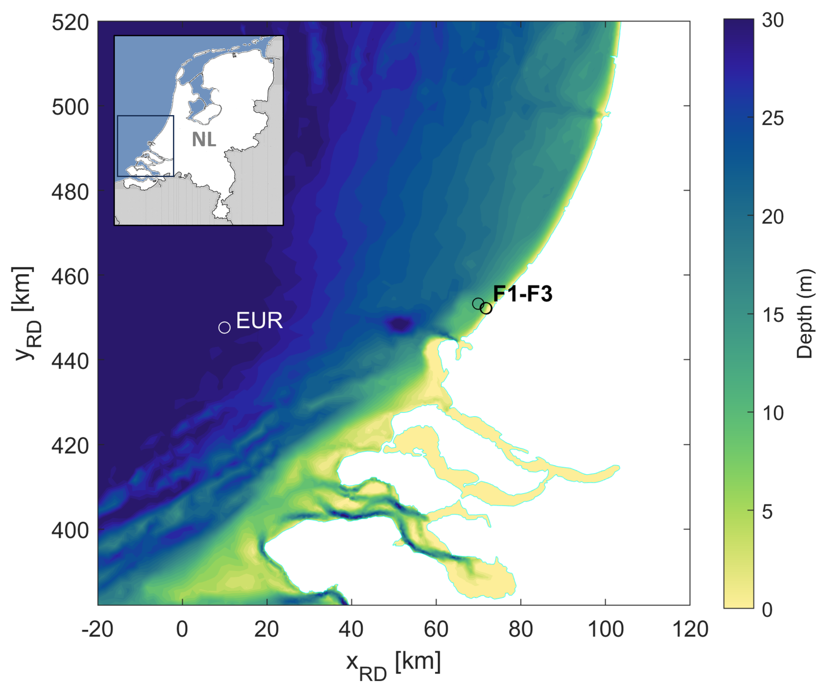
Figure 2.
(a) Bed elevation profile with location of measurement frames, (b) timeline indicating data collection periods of the different instruments. No velocity data were recorded at frame 3 after 21 February 2022.
Figure 2.
(a) Bed elevation profile with location of measurement frames, (b) timeline indicating data collection periods of the different instruments. No velocity data were recorded at frame 3 after 21 February 2022.
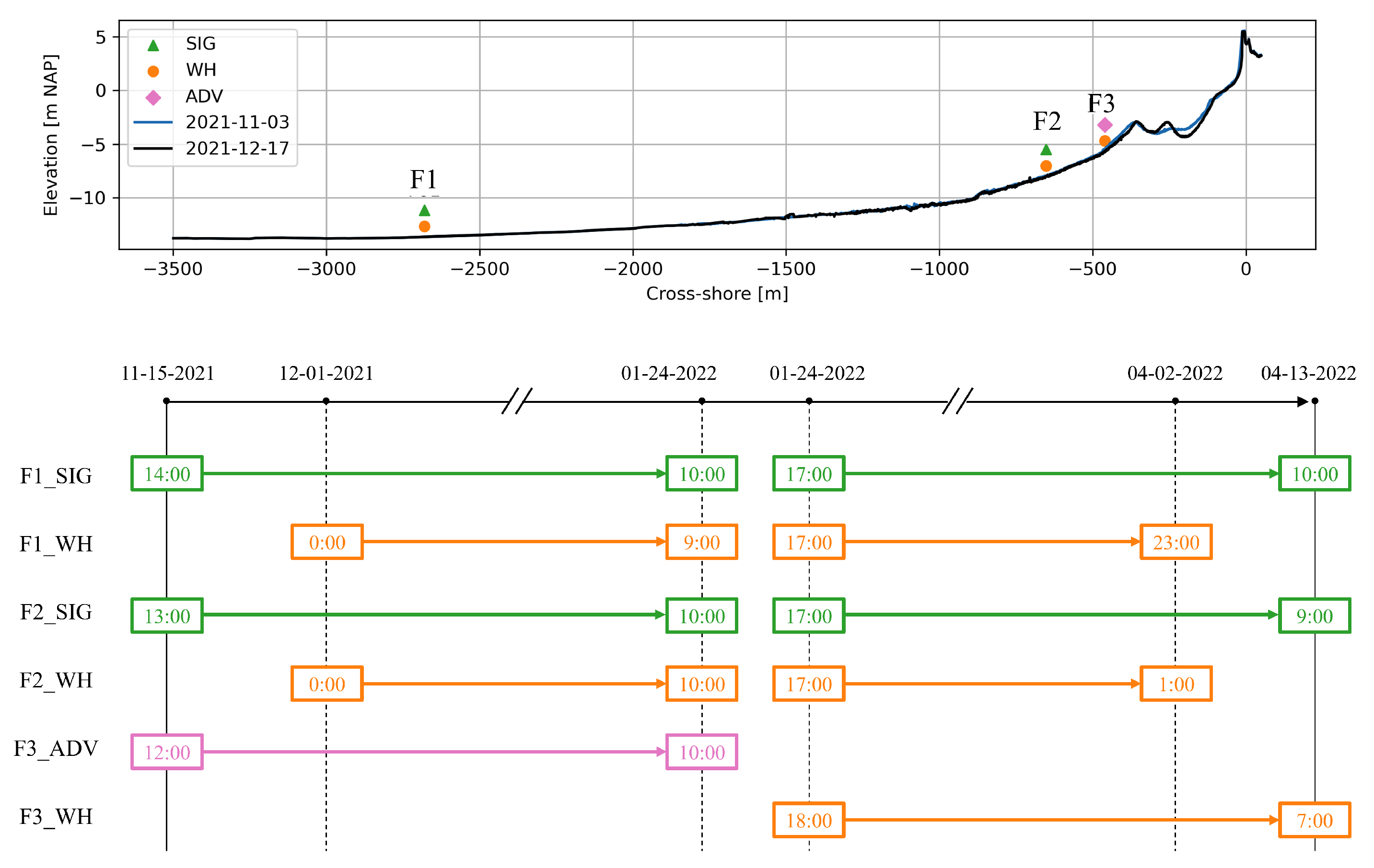
Figure 3.
(a) Frame 1 with Signature (SIG) and Workhorse (WH) ADCPs, (b) Frame 2 with SIG and WH ADCPs, (c) Frame 3 Vector ADV deployed from 15 November 2021 - 24 January 2022, and (d) Frame 3 with WH ADCP deployed 24 January 2022 - 13 April 2022. Red arrows indicate velocity (vel) and pressure (p) sensor heights from the bottom as indicated in Table 2.
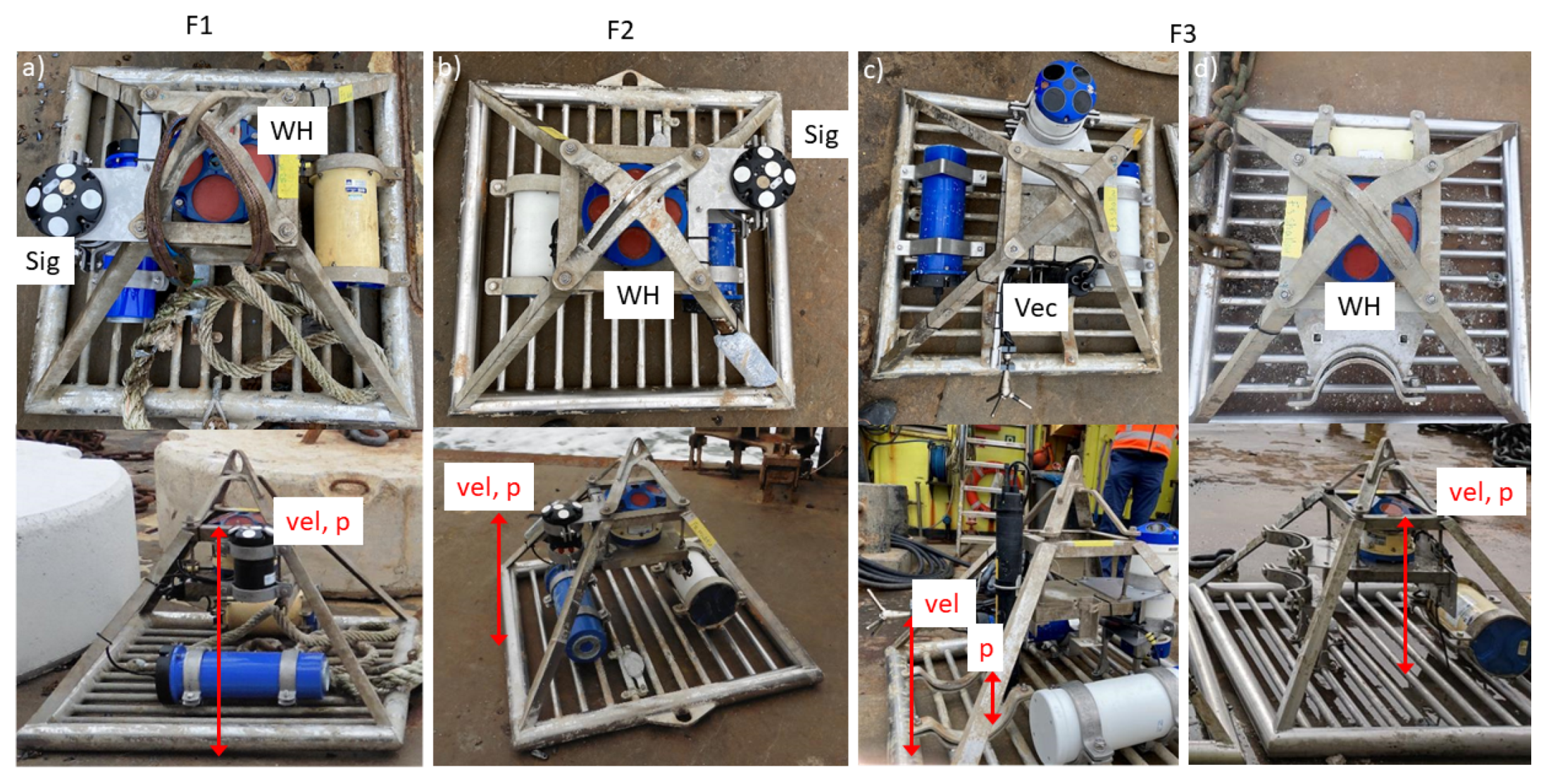
Figure 4.
(a-b) The cantilever bent and the ADV velocity probe got out of position, (c) heading measured in the housing of the ADV, (d) instantaneous X (blue), Y (red) and Z (yellow) velocity in the ADV coordinate system and (e) corresponding 10-min averaged velocity.
Figure 4.
(a-b) The cantilever bent and the ADV velocity probe got out of position, (c) heading measured in the housing of the ADV, (d) instantaneous X (blue), Y (red) and Z (yellow) velocity in the ADV coordinate system and (e) corresponding 10-min averaged velocity.
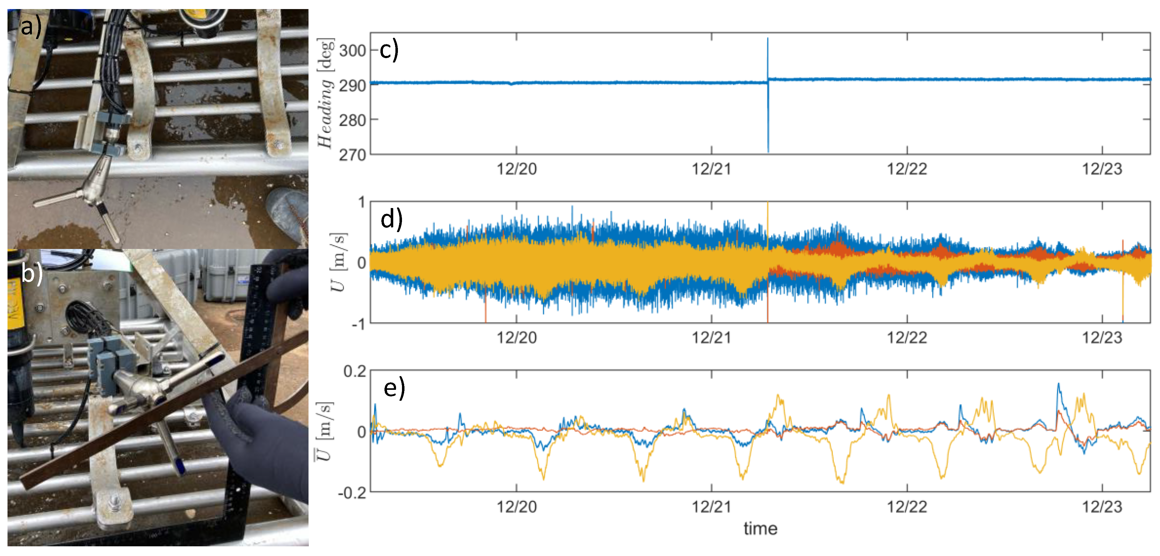
Figure 5.
(a) Example of water level drop in the instantaneous water depth measured with acoustic surface tracking. , at F1 by the Signature ADCP on 21 February 2022. (b) Example of containing spikes (blue) and with spikes removed (gray) at F1 on 31 January 2022 (storm Corrie; Table 8). Flagged data points were set to NaNs and no interpolation was performed in the despiked time series.
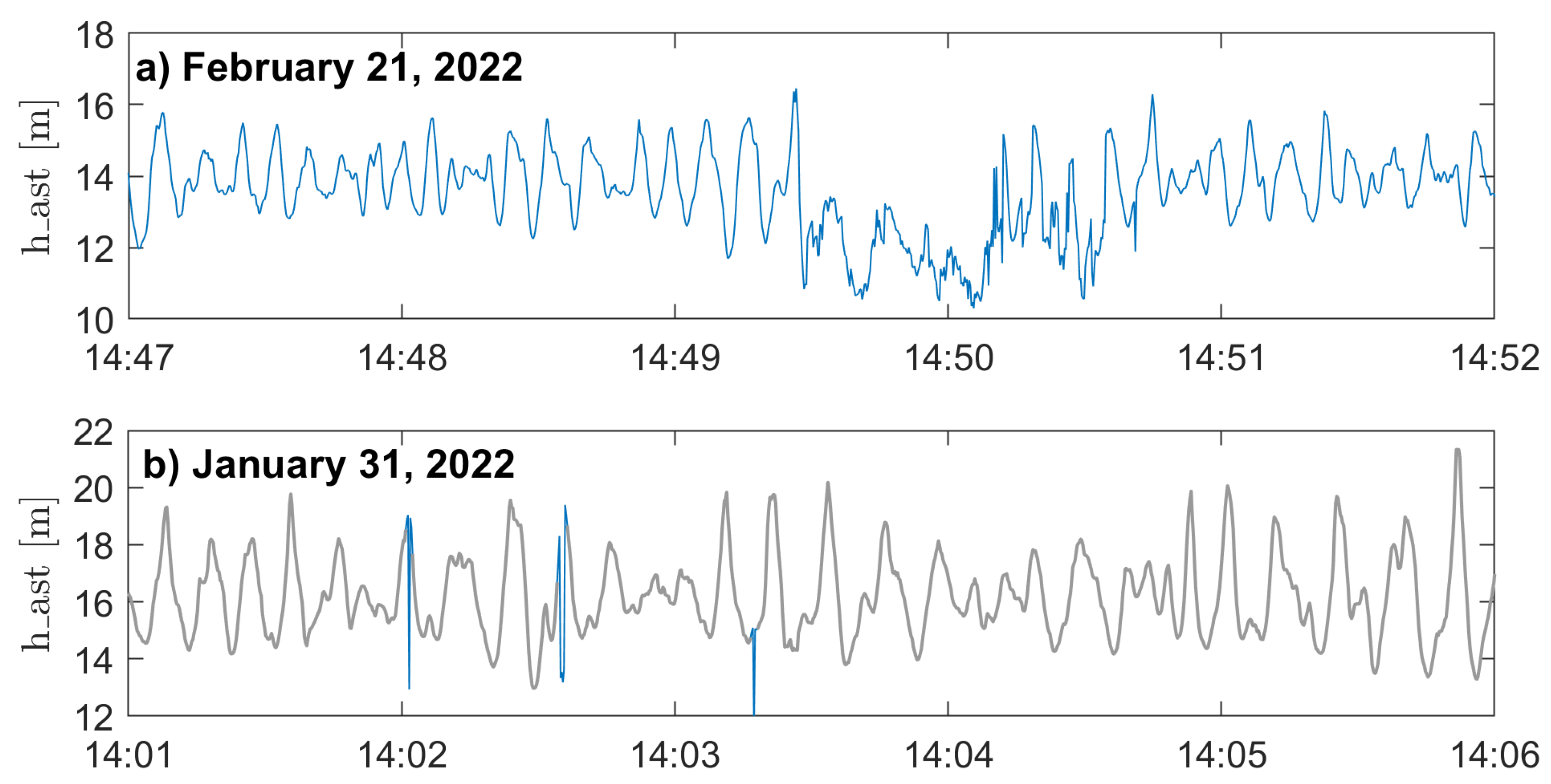
Figure 6.
Velocities along Beam 1 10.2 m from the bottom for the Signature ADCP at frame 1 (F1) on 5 January 2022. (a) Raw velocity during the entire day showing the semi-regular occurrence of periods with pronounced spikes. (b) and (c) Zoom of two 5-min subsets with raw (blue) and despiked (gray) time series. Flagged data points were set to NaNs and no interpolation was performed. Asterisks in (a) indicate the selected 5-min subsets.
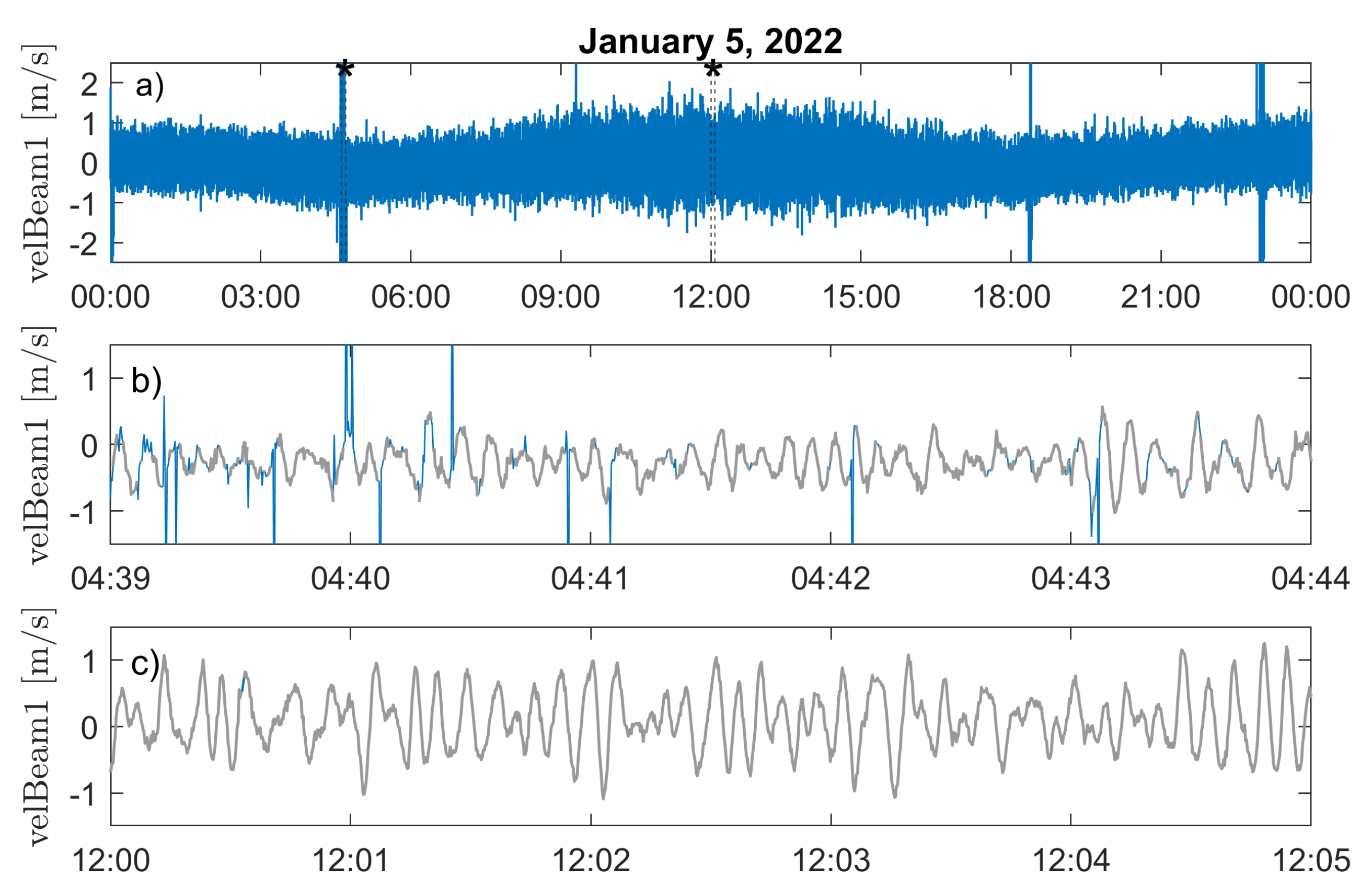
Figure 7.
Percentage of flagged data due to (a) low correlations and due to (b) spikes in the velocity time series for the Signature ADCPs at frame 1 (blue) and frame 2 (red), and the Vector ADV (yellow) and Workhorse ADCP (green) at frame 3. Vertical dashed lines indicate the minimum and maximum 1-hr averaged water depth.
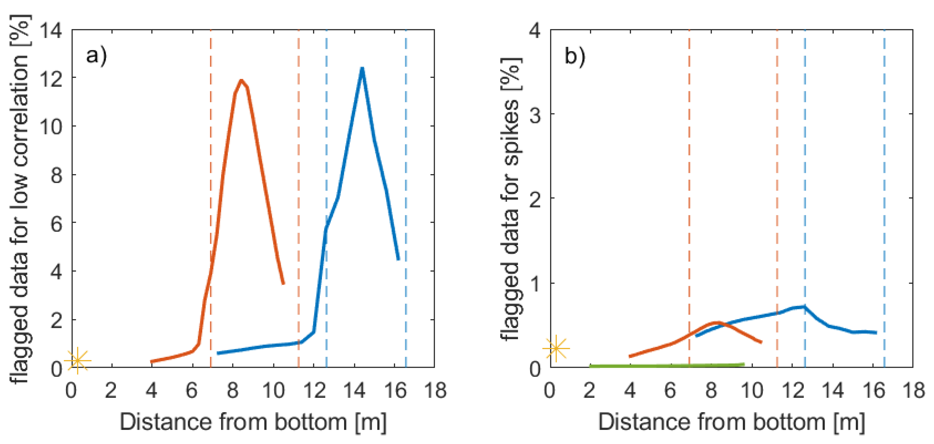
Figure 8.
Hydrodynamic conditions during the 5-month study period at F1 (blue), F2 (red) and F3 (yellow) with (a) sea surface elevation spectrum at frame 1, (b) sea-swell significant wave height , (c) infragravity significant wave height , (d) mean wave period , (e) sea-swell mean wave direction , and (f) 1-hr averaged water depth. The dashed horizontal red lines in (a) indicate the limits of the IG and SS frequency bands, whereas the dashed black line in (e) indicates the shore-normal corresponding to the local coastline orientation. Note that no directional information is available for F3 after February 2022.
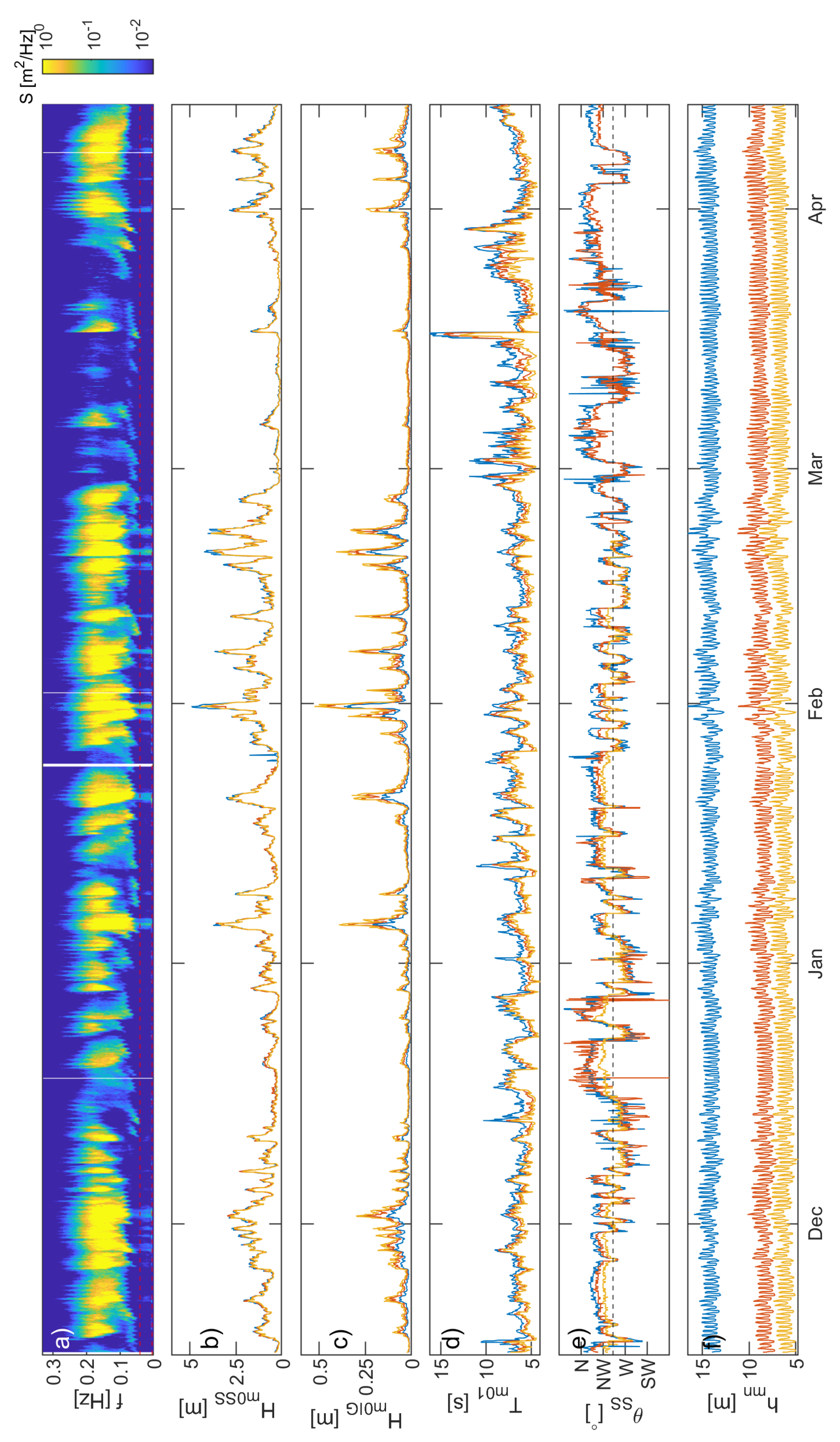
Figure 9.
Wave roses during the 5-month study period at (a) Europlatform, (b) F1, (c) F2, and (d) F3. The dashed horizontal red lines indicate the shore-normal direction corresponding to the local coastline orientation (295 deg N).
Figure 9.
Wave roses during the 5-month study period at (a) Europlatform, (b) F1, (c) F2, and (d) F3. The dashed horizontal red lines indicate the shore-normal direction corresponding to the local coastline orientation (295 deg N).
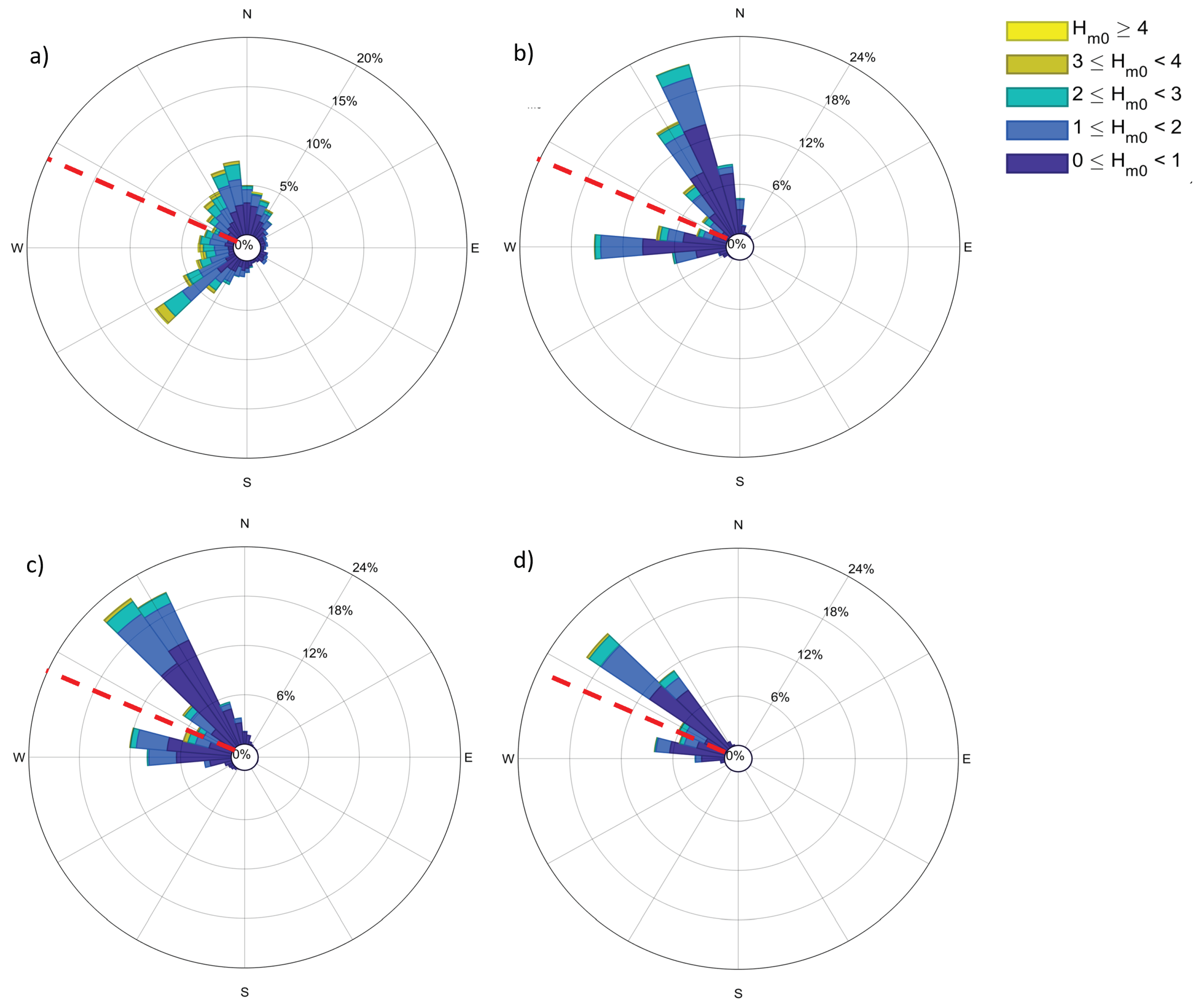

Table 1.
Position of three bottom frames in RD coordinate system.
| Setting | Offshore frame F1 | Middle frame F2 | Shallow frame F3 |
|---|---|---|---|
| Bed elevation | -14.4 m MSL | -8.6 m MSL | -5.8 m MSL |
| , | 69915 m, 453244 m | 71667 m, 452203 m | 71844 m, 452128 m |
Table 2.
Deployment settings of Signature 1000 ADCPs.
| Setting | Offshore frame F1 | Middle frame F2 |
|---|---|---|
| Sampling plan | Average & Wave height and direction | Average & Wave height and direction |
| Frame depth | -14.4 m MSL | -8.6 m MSL |
| Velocity range | 5 m/s | 5 m/s |
| Sensor height from bottom | 0.6 m | 0.6 m |
| Wave height and direction sampling | ||
| Cell size | 0.6 m | 0.3 m |
| Blanking distance | 6 m | 3 m |
| Number of cells | 18 | 23 |
| Sampling frequency | 4 Hz | 4 Hz |
| Number of pings | 1 | 1 |
Table 3.
Deployment settings of Workhorse ADCPs.
| Setting | Offshore frame F1 | Middle frame F2 | Shallow frame F3 |
|---|---|---|---|
| Frame depth | -14.4 m MSL | -8.6 m MSL | -5.8 m MSL |
| Velocity range | 3.0 m/s | 3.0 m/s | 3.0 m/s |
| Sensor height from bottom | 0.6 m | 0.6 m | 0.6 m |
| Cell size | 0.70 m | 0.35 m | 0.35 m |
| Blanking distance | 1.47 m | 0.74 m | 0.74 m |
| Number of cells | 35 | 52 | 39 |
| Waves | |||
| Sampling frequency | 2 Hz | 2 Hz | 2 Hz |
| Number of pings | 1 | 1 | 1 |
| Time between start of burst | 2 hr | 2 hr | 2 hr |
| Burst duration | 1 hr | 1 hr | 1 hr |
Table 4.
Deployment settings of Vector ADV.
| Setting | Shallow frame F3 |
|---|---|
| Frame depth | -5.8 m MSL |
| Velocity range | 7.0 m/s |
| Pressure sensor height from bottom | 0.08 m |
| Velocity sensor height from bottom | 0.28 m |
| Sampling frequency | 4 Hz |
Table 5.
Variables collected at frames 1 and 2 (F1, F2) by Signature 1000 ADCP.
| Variable name | Size | Long name [unit] |
|---|---|---|
| time | time x 1 | Time [seconds since 1970-1-1 00:00:00 UTC] |
| height_cell | height_cell x 1 | Height of cell center from the bottom [m] |
| p | time x 1 | Raw pressure [dBar] |
| p_apc | time x 1 | Pressure corrected for air pressure and offset [Pa] |
| h_ast | time x 1 | Vertical distance from sensor to surface, from acoustic surface tracking [m] |
| h_le | time x 1 | Vertical distance from sensor to surface, from leading edge [m] |
| velEast | time x height_cell | Flow velocity of water in east-direction, positive is going to the east [m/s] |
| velNorth | time x height_cell | Flow velocity of water in north-direction, positive is going to the north [m/s] |
| velUp | time x height_cell | Flow velocity of water in up-direction, positive is going up [m/s] |
| velBeam1 | time x height_cell | Flow velocity of water in Beam1-direction, positive is going in direction of beam [m/s] |
| velBeam2 | time x height_cell | Flow velocity of water in Beam2-direction, positive is going in direction of beam [m/s] |
| velBeam3 | time x height_cell | Flow velocity of water in Beam3-direction, positive is going in direction of beam [m/s] |
| velBeam4 | time x height_cell | Flow velocity of water in Beam4-direction, positive is going in direction of beam [m/s] |
| corBeam1 | time x height_cell | Correlation of Beam 1 [%] |
| corBeam2 | time x height_cell | Correlation of Beam 2 [%] |
| corBeam3 | time x height_cell | Correlation of Beam 3 [%] |
| corBeam4 | time x height_cell | Correlation of Beam 4 [%] |
| ampBeam1 | time x height_cell | Amplitude of Beam 1 [dB] |
| ampBeam2 | time x height_cell | Amplitude of Beam 2 [dB] |
| ampBeam3 | time x height_cell | Amplitude of Beam 3 [dB] |
| ampBeam4 | time x height_cell | Amplitude of Beam 4 [dB] |
| flag_data | time x 1 | Flag vector with 0’s indicating when the instrument was not in the water |
| flag_h_ast | time x 1 | Flag vector with 0’s indicating spikes and 2’s indicating 1-hr bursts with erroneous drops in h_ast |
| flag_vel | time x height_cell | Flag vector with 0’s indicating low correlation or spikes in velocity for Beams 1-4 |
| heading | time x 1 | True heading, corrected for deviation of magnetic from true north [deg clockwise from north] |
| pitch | time x 1 | Pitch [deg] |
| roll | time x 1 | Roll [deg] |
| temperature | time x 1 | Sea water temperature [Celcius] |
Table 6.
Variables collected at frames 1, 2 and 3 (F1, F2, F3) by Workhorse ADCPs.
| Variable name | Size | Long name [unit] |
|---|---|---|
| time | time x 1 | Time [seconds since 1970-1-1 00:00:00 UTC] |
| height_cell | time x height_cell | Height of cell center from the bottom [m] |
| p | time x 1 | Raw pressure [m] |
| p_apc | time x 1 | Pressure corrected for air pressure and offset [Pa] |
| h_ast | time x 4 | Distance from sensor to surface along slanted beams 1-4, from acoustic surface tracking [m] |
| velEast | time x height_cell | Flow velocity of water in east-direction, positive is going to the east [m/s] |
| velNorth | time x height_cell | Flow velocity of water in north-direction, positive is going to the north [m/s] |
| velUp | time x height_cell | Flow velocity of water in up-direction, positive is going up [m/s] |
| velBeam | time x 4 x height_cell | Flow velocity of water in Beam 1-4 direction, positive is going in direction of beam [m/s] |
| flag_data | time x 1 | Flag vector with 0’s indicating when the instrument was not in the water |
| flag_vel | time x height_cell | Flag vector with 0’s indicating spikes in velocity for Beams 1-4 |
| time_hpr | time_hpr x 1 | Time corresponding to heading, pitch, roll data [seconds since 1970-1-1 00:00:00 UTC] |
| heading | time_hpr x 1 | True heading, corrected for deviation of magnetic from true north [deg clockwise from the north] |
| pitch | time_hpr x 1 | Pitch [deg] |
| roll | time_hpr x 1 | Roll [deg] |
| temperature | time_hpr x 1 | Sea water temperature [Celcius] |
Table 7.
Variables collected at frame 3 (F3) by Vector ADV.
| Variable name | Size | Long name [unit] |
|---|---|---|
| time | time x 1 | Time [seconds since 1970-1-1 00:00:00 UTC] |
| p | time x 1 | Raw pressure [Pa] |
| p_oc | time x 1 | Pressure corrected for pressure offset [Pa] |
| p_apc | time x 1 | Pressure corrected for air pressure and offset [Pa] |
| velX | time x 1 | Flow velocity of water in x-direction [m/s] |
| velY | time x 1 | Flow velocity of water in y-direction [m/s] |
| velZ | time x 1 | Flow velocity of water in z-direction [m/s] |
| velEast | time x 1 | Flow velocity of water in east-direction, positive is going to the east [m/s] |
| velNorth | time x 1 | Flow velocity of water in north-direction, positive is going to the north [m/s] |
| velUp | time x 1 | Flow velocity of water in up-direction, positive is going up [m/s] |
| corX | time x 1 | Correlation of Beam 1 [%] |
| corY | time x 1 | Correlation of Beam 2 [%] |
| corZ | time x 1 | Correlation of Beam 3 [%] |
| snrX | time x 1 | Signal-noise ratio of Beam 1 [%] |
| snrY | time x 1 | Signal-noise ratio of Beam 2 [%] |
| snrZ | time x 1 | Signal-noise ratio of Beam 3 [%] |
| flag_data | time x 1 | Flag vector with 0’s indicating when the instrument was not in the water |
| flag_vel | time x 1 | Flag vector with 0’s indicating low SNR, low correlation or spike |
| time_hpr | time_hpr x 1 | Time corresponding to heading, pitch, roll data [seconds since 1970-1-1 00:00:00 UTC] |
| heading | time_hpr x 1 | True heading, corrected for deviation of magnetic from true north [deg clockwise from the north] |
| pitch | time_hpr x 1 | Pitch [deg] |
| roll | time_hpr x 1 | Roll [deg] |
| temperature | time_hpr x 1 | Sea water temperature [Celcius] |
Table 8.
Wave characteristics at F1 during the peak of the nine storms identified during the study period. Sea surface elevation was obtained from the tidal stations.
Table 8.
Wave characteristics at F1 during the peak of the nine storms identified during the study period. Sea surface elevation was obtained from the tidal stations.
| Date | Hm0SS [m] | Hm0IG [m] | Tp [s] | thetaSS [] | [m MSL] | |
|---|---|---|---|---|---|---|
| Storm 1 | 1-Dec | 2.9 | 0.14 | 11 | 324 | 2.1 |
| Storm 2 | 5-Jan | 3.7 | 0.21 | 10 | 320 | 2.3 |
| Storm 3 | 20-Jan | 3.1 | 0.17 | 13 | 334 | 1.7 |
| Storm 4 (Corrie) | 31-Jan | 5.0 | 0.37 | 12 | 319 | 2.9 |
| Storm 5 | 7-Feb | 3.7 | 0.18 | 11 | 318 | 1.9 |
| Storm 6 (Dudley) | 17-Feb | 3.2 | 0.13 | 9 | 290 | 1.5 |
| Storm 7 (Eunice) | 19-Feb | 4.2 | 0.25 | 10 | 281 | 2.1 |
| Storm 8 (Franklin) | 21-Feb | 4.1 | 0.21 | 9 | 289 | 2.5 |
| Storm 9 | 31-Mar | 2.9 | 0.12 | 9 | 348 | 1.3 |
Disclaimer/Publisher’s Note: The statements, opinions and data contained in all publications are solely those of the individual author(s) and contributor(s) and not of MDPI and/or the editor(s). MDPI and/or the editor(s) disclaim responsibility for any injury to people or property resulting from any ideas, methods, instructions or products referred to in the content. |
© 2024 by the authors. Licensee MDPI, Basel, Switzerland. This article is an open access article distributed under the terms and conditions of the Creative Commons Attribution (CC BY) license (http://creativecommons.org/licenses/by/4.0/).
Copyright: This open access article is published under a Creative Commons CC BY 4.0 license, which permit the free download, distribution, and reuse, provided that the author and preprint are cited in any reuse.


