
Submitted:
11 March 2024
Posted:
13 March 2024
You are already at the latest version
Abstract
This study investigates the historical variability in annual average precipitation in the northwest region of Mexico, aiming to evaluate the cumulative impact of precipitation on soil degradation and associated risks posed by rainfall. Despite being known as "The Agricultural Heart of Mexico," the region's soil has experienced significant damage to its granulometric structure due to unpredictable rainfall patterns attributed to climate change. Sixteen historical series of average annual rainfall were analyzed as stationary stochastic processes for spectral analysis. The results revealed exponential decay curves in each radial spectrum, indicating a linear relationship between frequency and amplitude. These curves identified initial impulses correlated with moments of severity for structural damages caused by rainfall-induced degradation. The degradation process, exacerbated by water stress, accelerates, as evidenced by maps illustrating approximately 75% soil damage. In the context of climate change and the uncertainty surrounding soil responses to extreme meteorological events, understanding this phenomenon becomes crucial. Recognizing the dynamic nature of soil responses to environmental stressors is essential for effective soil management. Emphasizing the need to employ numerical processes tailored to new environmental considerations related to observed soil damages is crucial for sustainable soil management practices in any region.
Keywords:
precipitation
; soil degradation
; climate variability
; spectrum and soil management
1. Introduction
Contemporary challenges facing Mexican agriculture, particularly in the northwest region, necessitate adaptation to meet evolving global market demands. The global market collapse in 2007 underscores the need for agricultural products to align with international standards. Concurrently, projections indicate a global agricultural growth requirement of 50% and 70% in developing countries, emphasizing the imperative of precise water and soil management [1,2]. In Mexico, historically engaged in numerous trade agreements, holds opportunities for sustainable and competitive agriculture. The recent North American Free Trade Agreement offers renewed prospects, calling for enhanced commercial engagement and environmental management plan restructuring. However, the compounding challenges of climate change exacerbate pressure on agricultural practices, particularly soil degradation, presenting a complex task for adaptation amidst globalization.
These levels of soil degradation in Mexico is result from various granulometric combinations by the distribution variation edaphic richness across its territory. Among the 32 known soil units, 25 are dispersed in microreliefs and microclimates with different types of vegetation [3]. This diversity contributes to multiple combinations of factors affecting and transforming soil structure, leading to the development of numerous methodologies and definitions to study it degradation [4]. The results, until now, are solely close approximations of the actual level of soil degradation.
The differences in soil degradation across the Mexican Republic are evident in the literature, as illustrated by two works from academic and governmental institutions with a shared goal of establishing a national baseline for soil degradation. One report indicates that 61.7% of the soil in the national territory is affected by erosions caused by water, wind, chemicals, physical factors, and soil withering, leading to degradation [5] (pp. 45-47), [6] (p. 31). Meanwhile, another study, at a 1:250,000 scale, provides a map and reports similar causes of soil degradation but attributes it to anomalous management practices, particularly with agricultural cover areas, revealing a 55% total degradation trend that could lead to erosion [7].
Consistent issues related to soil degradation have been reported across various dates, primarily linked to soil pressure during diverse land use activities, especially in agriculture. Despite variations in the degree of degradation observed in the studies, it is evident that adherence to current management practices poses a significant risk to soil granulometric structures, thus threatening long-term agricultural productivity and economic output.
Addressing the consequences of extreme meteorological events that rapidly damage soil, contemporaneous soil management plans are crucial, not only in Mexico but also urgently needed globally. The solutions emphasize the imperative development of new mechanisms for holistic agricultural land management, adding environmental value to products. This urgency is highlighted by the continued role of agriculture in contributing to approximately one-third of global greenhouse gas (GHG) emissions.
If it is accurate that continued adherence to traditional management practices in agriculture poses a severe risk to soil health, then it becomes evident that contemporary soil management plans are urgently required on a global scale. Emphasis should be placed on developing innovative mechanisms to enhance the environmental value of agricultural land use. This urgency is further compounded by agriculture's significant contribution to global GHG emissions.
Degradation of soil is intricately linked to the "perfect cycle of agricultural production," encompassing various emission phases from field activities to food processing and waste management [8,9]. This connection underscores the complexity and interdependence of agricultural activities, where each phase contributes to the overall environmental impact.
Recognizing the urgency of adapting to globalization and climate change, it is imperative to explore alternatives for functional and sustainable soil management globally. This emphasizes the development of mechanisms for comprehensive soil management that adds environmental value to agricultural products. Shifting towards sustainable practices is crucial to mitigate GHG emissions from agricultural activities, addressing the increasing demands of a globalized world.
Addressing these challenges necessitates urgent development and implementation of innovative strategies integrating environmental considerations into every stage of agricultural production. These strategies should not only reduce GEI emissions but also enhance overall sustainability, ensuring the well-being of populations globally [2]. Balancing food demands, mitigating environmental impacts, and guaranteeing population well-being is complex yet crucial for creating a resilient and sustainable agricultural system, especially in the zone “The Agricultural Heart of Mexico”, given the consistent year-round nature of its agricultural activities.
The current comprehensive management approach for soil conservation in Mexico necessitates new plans or adjustments. However, these plans must be equipped to control, counteract, and combat soil erosion effectively, utilizing precise data measures. Given the evolving conditions brought about by climate change, these plans need to be functional, tailored to specific areas, and developed based on long-term characterizations of soil behavior. The primary focus in this country should be on identifying the severity of consequences resulting from the impact of meteorological phenomena on soil, particularly those accumulating over time and causing rapid damage.
In response to the challenges of soil management amid globalization and climate change, the utilization of precise methodologies is crucial. Incorporating contemporary statistical and econometric tools in data analysis ensures decision-making based on information free from randomness associated with disturbances produced by the presence of autocorrelation (AC) and other behaviors that transform and mask real information due to its non-stationary stochastic process. This approach provides a level of certainty, enabling the exploration of high-probability scenarios with real and low-uncertainty information. Changes observed during soil evaluation processes are reliable, and the information obtained through these evaluations responds with less uncertainty to any adaptation, mitigation, or soil recovery strategy applied.
Therefore, this study aims to comprehend the consequences of rainfall-induced soil structural degradation in a pivotal Mexican economic area known for its high agricultural production.
Considering these guidelines, the study utilizing 51 years of the dataset from 16 signals temporals (St) historical from the average annual of precipitation () measured by the meteorological stations operated by CONAGUA (1961-2011), this study was employed a stochastic approach to assess the severity of consequences and risks associated with soil degradation. The prior analysis was conducted in the frequency domain to obtain variations in the power spectrum () for each St. A degree of radial integration was employed to estimate and graphically represent the radial spectral potential () for its respective St.
The analysis takes into consideration the region's ongoing historical exploitation, its high susceptibility to desertification processes, and the influence of North American monsoonal dynamics. It begins with the premise that relying on rigorously controlled and verified data is essential for developing effective agricultural management plans that address climate change, thus emphasizing the paramount importance of data quality. In this study, ensuring data quality is accomplished through the analysis of seasonal stochastic conditions. This approach enables the estimation of spectral potential and the regionalization of soil erosion risk, serving as a crucial indicator of soil granulometric state in relation to the cumulative risk posed by precipitation.
2. Materials and Methods
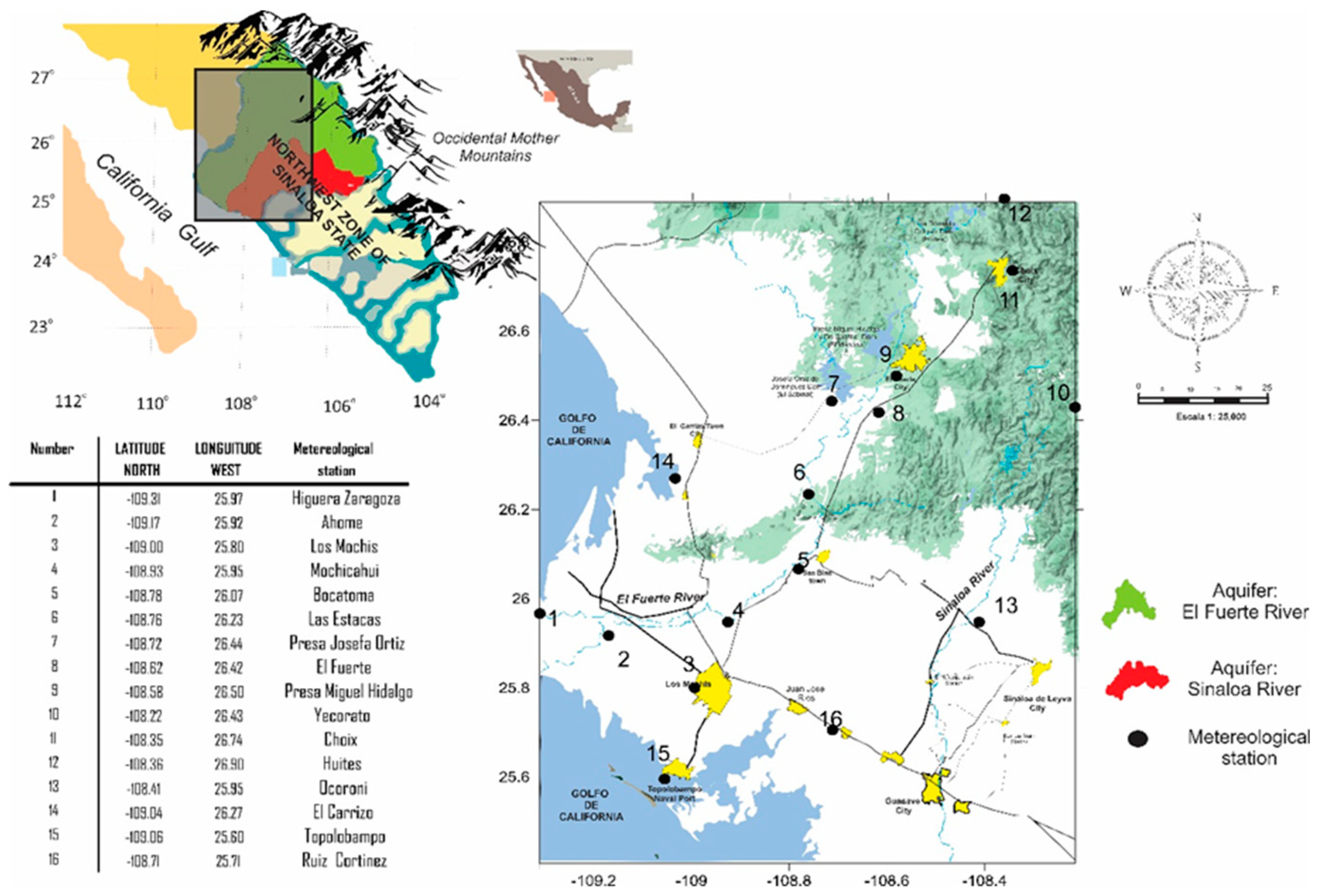
In the extensive coastal plain of Northwest Mexico, specifically in the state of Sinaloa, there are two interconnected agricultural valleys situated in the hydrographic basins of the “Río Fuerte” and “Río Sinaloa.” Renowned for their high productivity, these valleys play a crucial role in a territory where surface waters drain into the rivers of the same name as their respective basins (Figure 1). The origin of two rivers is in the high mountains of the Sierra Madre Occidental (SMO), both intersect the valley, and their flows vary seasonally, ultimately discharging into the Sea of Cortés, also known as the Gulf of California.
Within the Sinaloa River Basin lies a coastal region with diverse soil types that have been utilized for agriculture for many centuries, now commonly referred to as "The Agricultural Heart of Mexico." This agricultural legacy predates the Spanish conquest of the Mexican territory, with products cultivated by tribes such as the "Cahitas" and "Pimas bajos" for consumption and trade, encompassing a variety of crops.
This historical significance propelled the region into becoming a priority exporter of cotton worldwide during 1950s to 1970s. Adapting to the ideals of the "Green Revolution" in 1960s, the agriculture of the region underwent significant transformations to meet nutritional and economic needs. However, current challenges arise from climate change, affecting the physical, chemical, and biological properties of the soil. Given these challenges, it becomes crucial to comprehensively understand the risks posed by extreme weather phenomena, particularly focusing on the severity of consequences related to rainfall-induced soil structural degradation. This study aims to analyse the historical series of average annual precipitation to assess the potential risks and consequences, emphasizing the need for innovative and sustainable soil management practices in this vital agricultural region.
The soil in the region played a pivotal role in meeting global cotton demands from 1920s to 1970s, establishing itself as a priority exporter worldwide, particularly during the 1950s to 1970s. This raw material became a strategic pillar of the Mexican state's economy throughout various periods in the 20th century [10]. Evolving with the ideals of the "Green Revolution" in 1960s, the subsequent decades witnessed a transformation from intensive to technical agriculture. The primary mission was to meet the nutritional and economic needs of the region's inhabitants and the broader Mexican population.
Figure 1.
Displays the location and weather stations in the coastal plain and mountainous areas of Northwest Mexico, highlighting the productive soils of the “River El Fuerte” and “River Sinaloa” hydrographic basins, known as "The Agricultural Heart of Mexico" zone.
Figure 1.
Displays the location and weather stations in the coastal plain and mountainous areas of Northwest Mexico, highlighting the productive soils of the “River El Fuerte” and “River Sinaloa” hydrographic basins, known as "The Agricultural Heart of Mexico" zone.
While the agricultural practices of 1960s contributed to sustaining a growing global population, contemporary challenges arise from environmental scenarios shaped by climate change, introducing variable physical, chemical, and biological properties to the soil. The historical agricultural exercise operated under evolving circumstances in each epoch, considering environmental, political, and social factors. Undoubtedly, the pressure on soils was subjected to various strategic aspects crucial for the growth of the Mexican economy, with undeniable regional impacts on the soil. Now, faced with intensified and constant weather phenomena in recent decades, there is a critical need to understand the variability of potential consequences and risks of soil degradation. This study aims to explore the severity of these consequences, emphasizing the importance of comprehending the impacts of variable meteorological phenomena on soil in the current environmental context [11].
In this study, we analysed the severity of consequences on agricultural soil, with a specific focus on rain as a significant factor with varying potential to cause erosion or complete soil loss. To assess both the total precipitation accumulated over time () its damages to the soils, was examined Sts of from 16 meteorological stations operated by CONAGUA. The emphasis was placed on rain-induced degradation in the internal granulometric structure of the soil, typically occurring within the first 7 to 30 minutes of rainfall. These early stages represent the highest risks due to the substantial energy carried by rain, resulting in significant alterations to the soil's internal granulometric structure.
For a precise understanding of the severity of soil damage, it was crucial to utilize only temporally stationary information as a condition in the numerical process for all Sts. The analysis began with the characterization and familiarization of each historical series, considering that the information is the results from a combination of stochastic processes, which may be stationary or non-stationary at some point. The transformation of weather station information from non-stationary to stationary involves obtaining as a signal composed of sines and cosines over time, with differences in amplitude and frequency.
Adhering to this, the use of a stationary signal was considered obligatory for determining and , as spectral analysis of any harmonic process requires that signals have to been stationaries [12].
This guarantees that the analysis is based on real stationary information in the frequency domain, allowing the determination precise of the potential spectrum of and subsequently the characterization of .
Given that not all the information in each St series necessarily had to be stationary, it was necessary to first detect which St series met the continuity criteria before applying a numerical process to obtain the signal of sines and cosines in each St. This process involved analysing the dataset of 16 St from CONAGUA (referred to as the original dataset from this point forward) to identify which of the Sts could meet the continuity criteria.
In this study, it was of utmost importance to ensure the integrity of stationarity in each St and its behavior, which is composed of sines and cosines. This measure guaranteed that the signal remained a composition of stationary cycles, free from any loss of information, discontinuities, or distortions. Such meticulousness was essential to prevent disruptions to the analysed harmonic structures. Moreover, the utilization of datasets with unchecked randomness during analysis could lead to overestimation and potentially obscure real behaviors. Randomness alters the internal structures of St, rendering it non-stationary, thereby complicating the determination of the true variability, especially during the initial moments when rainfall commences. This phase is critical as it corresponds to the period when the internal structure of the soil is most susceptible to damage from rainfall. The consideration of stationarity was therefore crucial, as neglecting it could not only influence each structure of St but also impact the variabilities of [13].
The stationary condition allows for the determination of with reduced uncertainty, serving as the direct focus indicator for assessing the severity of consequences resulting from the cumulative impact of precipitation over time, leading to soil degradation and associated risks posed by rainfall.
On the other hand, to achieve greater precision in our results and alleviate the growing uncertainty in the 16 dataset, it was imperative to scrutinize the manner in which it were collected by sensors in the respective meteorological stations. It was observed that the common method for measurement the dataset could lead to significant variability in results. Reports suggest that this data sometimes exhibits similarities in time-measured information and displays an exponential decay of the AC function (ACF) as the time delay increases [14,15,16]. Despite this, explorations focused on ACF face limitations in the original correlation and the true self-regression functions, impacting the covariance matrix variation and hindering a thorough exploration using common statistical estimators of correlation. Consequently, it became necessary to analyse the potential presence of any AC immersed in each dataset using non-conventional statistical methods.
Regardless of the source, the "Potential Criterion of Randomness" was considered in order to encompass in the dataset the total probability of any irregularities introduced by randomness in each dataset. This recognition of the challenge arises from the potential transformation of this effect into real measures of true variabilities, starting from the moments that initiated the analysis of this historical annual average of .
As a consequence, if distortions are not analysed within the dataset, it could lead to an overestimation of information and obscure genuine behaviors. Therefore, in this study, the utilization of correlation modelling to investigate autocorrelation (AC) based on time-related measurements was deemed necessary. This choice was driven by the advantages of the time model, which does not necessitate iteration or subsequent calculation, unlike variance-covariance estimation [17,18]. Therefore, the identification of potential AC presence was pursued through physically traceable non-conventional statistical methods, considering the implications of signal correlations. This approach is anticipated to bolster confidence in the results by addressing this limitation, thus preventing discrepancies in statistical hypothesis tests for seasonal conditions from resulting in an erroneous stochastic model due to the oversight of AC.
To delve into physically traceable non-conventional statistical methods for determining AC, it was essential to prioritize an examination of each dataset individually through statistical diagnoses [18,19,20]. All datasets were graphed to detect any discontinuities or deviations [21]. This step was crucial to ensure that the simplifications made in modelling were not overly aggressive, thereby preserving fidelity to the quality standards established for describing a seasonal statistical process.
Specifically, the parameters used for individual statistical diagnoses on all datasets included punctual indicators of dispersion, asymmetry, and skewness. The punctual indicator obtained were: values minimum (min) and maximum (max), media (), median (). The statistical dispersion parameters comprised absolute range (Rabs), standard deviation (σ), variance (σ2), determination coefficient (R2), correlation coefficient (R) and non-determination coefficient ((k = 1 − R2). Additionally, the variations of asymmetry and kurtosis statistical parameters were respectively represented by: Swew_ and Kurt_ while positional statistical parameters included the 25th and 75th percentiles.
In order to uphold the quality standards of a stationary signal during evaluation, it was crucial to prioritize the removal of AC interference. This was accomplished by employing physically traceable, non-conventional statistical methods within a visual multivariate statistical analysis for identification.
To detect AC, a combination of conventional and physically traceable non-conventional statistical methods was employed. The conventional method utilized was Multiple Linear Regression (MLR), while the two non-conventional visual methods included Mantel's Correlation Scalogram (MCS) and Geometric Correlation of Ellipses (GCE), and finally the Variance Inflation Factor (t_stat_VIF). Specifically, in the analysis of 16 dataset employing t_stat_VIF, correlations were evaluated based on the inflation factor, which links the average variance, as described in [22,23]. The emphasis to using t_stat_VIF stemmed from its consistent and successful utilization across various works. It has been employed to derive confidence intervals for site velocities derived from the Global Navigation Satellite System (GNSS), as well as in meteorology/climatology, and soil contamination studies utilizing multivariate data, as reported in [24,25,26].
MLR analysis. Respect to Ahome station, R-squared (R2) value, served as the initial indicator of a probable presence of AC in dataset of Sts originals. In this context, % R2 represented the shared information between the St datasets, signifying correlation, while the non-determination coefficient (k = 1 − R2) indicated information devoid of correlation. The absence of correlation indicated by k or the correlation by R2 was considered a partial indicator because the MLR analysis, focusing solely on one magnitude, might overlook some degree of AC. This assumption indirectly suggests that there is no AC when the variables are correlated or not with another Sts. This implies that if there are any degrees of AC present in the dataset analysed, it could be embedded within the percentage of k or R2, making it challenging to detect. Therefore, it was recognized that specification errors might arise when trying to enforce the functionality of the model based solely on k or R2 for AC usage. Consequently, relying solely on k and R2 values to represent the percentage of information in correlation could overlook the presence of AC, thus increasing the likelihood of specification errors in the model [27]. This was the cause because the RLM results were considered as a partial and preliminary indicator for the presence of AC. However, it is acknowledged that at some point, the possibility of the incursion of mechanisms that produce disturbances in the percentage of k or R2 may prevail, potentially preventing its representation as a stationary stochastic process in the information. This ambiguity could lead to the mistake of rejecting the Ho hypothesis and ato ccepting the alternative H1 or vice versa. Furthermore, disturbances and truncations in Minimum Ordinary Square (MCO) could affect the determination of AC. Despite the ability to intuit AC through Fisher statistical probability contrasts (prob_F_stat) at a significance level of α = 0.05 [prob_ (F_stat) vs. α], the disturbances of MCO constrained the contrast for the analysis of AC. Therefore, considering the argument presented in [28] (pp. 3-5), k or R2 results were considered only as partial indicators of AC. To mitigate the anomalous effects in parameter estimation using MCO and achieve a more accurate identification of the AC phenomenon, we considered the criteria outlined in [29]. This involved incorporating outlier detection tests for examination and exploring alternative visual methods to clarify areas of AC within the original dataset. From the four statistical estimators used for to detect AC, two methods were employed for focusing on visual observation to determine AC within the context of 'AC time'. These methods involved detecting correlations and measuring the AC function (ACF) by comparing correlations between and within the original information of each St.
MCS analysis. This was the second method for verify the presence of information shared between and within of each St. This statistical estimator visually allowed, respect to the maximum percentage spatial distribution that R2 could acquire (R2 = 1 = 100%), for to configure a correlation respect to dataset of St Ahome. The principium for show a visual graphical of the shared information was performed with respect to a phased or self-regressive copy of the St itself in the form , where and the average of , and shows at the base of the triangle the consecutive way how the pairs of nominal values have in similarity each time that the St were compared to each other and in the same way for their original representation of each and own St.
MCR statistical algorithm through values nominals concentrates for to form anomalies identifying precisely areas where there is either a correlation or an AC accumulated. The anomalies of AC were distributing over the basis of the triangle and below of this same base were illustrates the anomalies of correlation between the Sts. The simple correlation was observed in MSC as a distribution in percentage of R2 values scattered inside and over the base. The percentage R2 values on the base were the indicators that would be inside the own St autocorrelated, i.e., such as it is shared the variance in the own dataset.
GCE analysis: This method represented the third approach used to verify AC, which involved forming a triangle using different geometric figures, primarily trending towards ellipses and/or circles. The presence of a trend towards ellipses indicated a correlation within the triangle and, consequently, the presence of AC was defined by geometric figures tending towards an ellipse at the base of this triangle. Similarly, the trend towards forming a circle indicated information that did not share its σ2. This qualitative method, akin to MSC, visually detected the presence of AC by identifying the ellipses in the based with the number of signals indicating AC. These observations facilitated the appropriate adjustments needed to eliminate this AC behavior.
t_stat_VIF analysis: This method served as the fourth approach to verify, through the coefficient t_stat_VIF and P_value, whether the results of RLM could be confounded due to multicollinearity in each St. The probable presence of AC was indirectly associated by contrasting the sstical t_stat_VIF (calculated in each St) with the significance level t_stat_VIF > 10. If the value was exceeded stat_VIF > 10, it indicated a significant self-correlation problem. Therefore, t_stat_VIF < 10 suggested the absence of this self-correlation, rendering the problem irrelevant, and signifying that at least 75% of the information is not shared. Given the statistical simplicity of obtaining the t_stat_VIF indicator in this method, it was one of the selected approaches to verify seasonality both before and after the respective adjustments.
The St identified with AC through the four above methods were processed to eradicate randomities or noises in order to obtain seasonal stochastic processes over time. This involved minimizing the potential changes that could have occurred prior to the randomities affecting the behavior of the measurements used. The aim was to obtain processes that adhere to the properties of stationary conditions, ensuring consistency in the behaviors of measured nominal values. This enables them to either increase or decrease relative to a constant value.
Was considered that among the signals, there might be some randomness, which some authors define as a product of perturbations produced by the temporal evolution noise of any local source or by implications of regional climate change. However, this randomness relation, which could allow for a portion of spectral analysis to estimate magnitudes and evolutions of climate change on the zone, was not utilized here. It is only mentioned to define it as the difference of information separated from the dataset and used for the spectral analysis. This was significant in using information without randomness and conditioning its nominal values to be stationary. Overall, during the phase when results are interpreted, it is important to ensure that true behaviors related to damages yielded by variable rainfall cycles are accurately understood and conveyed.
These random effects on St could result in misinterpretations and erroneously associate phenomena that do not actually exist, thus deviating from the real conditions observed in rainfall patterns. To address these random processes, the original St was decomposed using the "Seasonal and Trend Decomposition Using Loess" (STL-Decomposition) method.
Subsequently, the verification of the possible presence of AC was conducted once again using the same ellipse method described here. In this new visual analysis, if changes from ellipses tending towards circular forms are observed, it suggests that the issue of AC in percentage terms has been addressed. Likewise, this information from the STL-Decomposition was corroborated in the absence of AC by contrasting [stat_VIF vs. VIF > 10].
The thorough verification of AC in St was conducted with the aim of ensuring complete confidence that the internal St did not share any part of their variance. However, with the distortions due to randomness eradicated through the ST-Decomposition adjustment, it can now be firmly asserted that the results of the spectral analysis, once transformed into the domain of frequencies exclusively stem from seasonal stochastic processes, either within the original St themselves or within some of their correlations.
To explore the dataset of original Sts and assess their seasonality, the afore mentioned statistical characterization criteria were employed. These criteria ensured that the Sts were conditioned to exhibit stochastic stationary behaviors with the expression (xi1, t1)j ……, where , and that their nominal values had to be different in each St and in the sequence of ……, , so that if in any of the values h > 0 it would be marked an apparent difference that could during the visual inspection identify a behavior as and which it is associated with this non-stationarity, and could erroneously be stationary but not in the original St if not in an autoregressive analysis of the original St itself.
So, as an alternative way to locate conditions that qualify with seasonality, it was taken into account in the mechanisms for verifying the properties of the statistical parameters mentioned above but now applied to an auto-regressive analysis of each original representation of the St of the form , to verify whether in this phased-out representation at the beginnings of the dynamic , here was a possibility of locating in , behaviors of and , similar to non-stationary behavior with a tendency to unity, resulting in its equivalence to the characteristic square unitary I(1) in the characteristic equation . So, the absence of I(1) in this characteristic equation anterior and its association with non-seasonality were properties that were explored to accomplish the combination of the first two criteria for the presence and/or absent I(1). The exploration on original representation of St, with its first and second self-regressive model were verify for analyse if in any of the cases the condition of seasonality was presented and if in any case was exist I(1), then the St was considering as a signal with seasonality.
However, before applying the algorithm to estimate these properties, in both criteria, it was important to condition the absence of AC in the information of each St:
- If any St, in its respective dataset original and self-regressive representation , exhibit a tendency towards unity in the absence of autocorrelation, equivalent to has present I(1) in the characteristic equation m, then it represent a non-stationary stochastic process, where its statistical parameters are defined with an average of and .
- If any St, in its respective dataset original and it same previous self-regressive representation in absence of AC, does not present a tendency to the unit, equivalent to the absences of I(1) in the same characteristic equation . then it is a stationary stochastic process and its statistical parameters will be represented in the form and .
Therefore, to apply both criteria and determine the presence or absence of I(1) within each dataset was used an analysis I(1) in levels, and if necessary, in its first or second self-regression (first difference and second difference analysis), it was essential to utilize the statistical estimator Augmented Dickey Fuller Test (t_stat_DFA). However, its use was conditioned strictly to effectively eliminate the presence of AC in each dataset. The aim to eradicate AC was crucial because the origins of observations are directly related to temporal nature dependence, randomness, and disturbances in the original data. This importance was considered because if any of its regressors could have AC, its mere presence would cause the original dataset to fail to meet the previous basic criteria of seasonality condition.
Accepting the AC levels to will use in the models, stationary certainty was confirmed in the series with the critical level contrast of 3.5% with the t_stat_DFA result. This eventually led to accepting or rejecting any of the Ho and H1 hypotheses, indicators of the seasonal or non-stable state of the St. The t_stat_DFA results were considered with the critical level of 5%, and the results of stat_Prob with the level of significance α = 0.05.
To avoid invalidating the R2 value result obtained by RLM tests, and to prevent working with a spurious RLM within of t_stat_DFA, once again, precaution was taken when obtaining the result without the possible presence of some AC has been filtered at some point not identified with the initial detection. A first-level exploration on first differences (PED) or second-level or second differences (SED) was performed to consider the following: "If a St has an I(1), then the PED and SED of such series will take the form of a non-stable static process”. So, if I(1) exists in the first or second difference, then the original dataset analysed will simply not be stationary.
Therefore, a PED was applied to determine whether the originals Sts met the zero hypothesis (Ho) when presenting I(1) (Ho = a =1) associated with non-stationarity. The contrast result of t_stat_DFA was not accepted without conducting another previous AC contrast with the Test Statistical Durvin Watson (t_stat_DW), also performed through the t_stat_DFA algorithm and considering its results within the limits established in the range R = [1.85, 2.15]. With this inclusion, the absence of AC in the model was affirmed with full certainty, thereby automatically validating its relevance when using t_stat_DFA to analyse the presence or absence of seasonality in the series.
In all St, statistically identified outliers were corrected thoroughly for the guarantees of working in the domain of time and frequencies with a set system of stationary stochastic processes represented with functions with simple, continuous, periodic, and symmetrical behavior of one mechanic wave in the form , where Aij was the amplitude of dataset, the angular frequency respect to time and θ the level of deface.
The deterministic simple of mechanic wave representations of each dataset allowed their numerical adjustment with the Fourier series by a trigonometric polynomial, assuring with the greatest possible weight that the uncertainty in the approximate representation of their nominal values in the directions xi and yj through the sines and cosines was reduced, and their behavior in 2D was in the form with ; which, by being integrable in the limits -π to π, allowed obtaining the nominal values in the directions xi and yj respectively for xi with the expression and for yj with .
This numerical approximation, employing sines and cosines formed by the nominal values of St through the principles of 2D Fourier series, facilitated the transformation from the time domain to the frequency domain [] using the Fourier Transform (FT).
The adjustment made to the information to obtain a stationary signal and utilize it in spectral analysis, following the criteria outlined in [30] (pp. 2189-2190), allowed for the fulfilment of requirements. This spectral estimation indicates that information must exhibit stationary behavior in all respects to facilitate a proper understanding of the source and the properties that generate // and //.
Therefore, the sine and cosine signals in the frequency domain, exhibiting stationary behavior, provide high guarantees for Fast Fourier Transformation (FFT). This allows us to determine, with confidence, the spectrum of in the directions r and θ for each St, represented in a regular mesh of m x n = 15 x 10, comprising 150 finite elements. The mesh in the zone represents the numerical matrix of variation as a stationary stochastic process in the frequency domain. The 2D representation of // is obtained through radial integration of //, followed by the assessment of the intensity of its initial impulses associated with the first moments when rain occurs at each meteorological station.
As insufficient information was available to characterize the spatial variation of , //, first impulses of / and the gravity indices of the consequences of these initial values of rain power that are incising on the soil; it was necessary to interpolate the respective results between neighbouring stations with kriging regular method [31] (pp. 613-615), and considering that several authors have demonstrated, unlike other techniques; that use of geostatistical methods obtain better estimates with interpolations, there are justifications such as those used here for to determine the behavior of / and // [32,33,34].
Therefore, in order to apply both criteria and to determine the presence and/or absence of I(1) in the St itself (analysis at levels), and if necessary, in its first or second self-regression (first difference and second difference analysis), it was necessary to eradicate the high probability of self-correlation presence in each St. Since, due to the temporal nature of its observations, it is directly related to the disturbance of the original data and equally, if any of its regressors have it, its presence was considered to be the cause of the failure to meet the previous basic criteria of seasonality condition.
Accepting the AC levels to be used in the models, stationary certainty was confirmed in the series with the critical level contrast of 3.5% and the t_stat_DFA result. This eventually led to accepting or rejecting any of the Ho and H1 hypotheses, indicators of the seasonal or non-stable state of the St. The t_stat_DFA results were contrasted with the critical level of 5%, and the results of stat_Prob with the level of significance α = 0.05.
The adjustments made to the information to obtain stationary signals allow us to use spectral analysis to meet the criteria outlined in [30]. It is emphasized that signals, in all respects, must exhibit stationary behavior to ensure a proper inference of the source and the properties that generate // and ///.
Thus, the guarantees in the result obtained with the Fast Fourier Transformation (FFT) to know in the directions r and θ to the spectrum of // of each St on a regular mesh m x n= 15 x 10 with 150 finite elements were established. The mesh divided the zone and represented the variation of as a stationary stochastic behavior process in the frequency domain where // was obtained, and subsequently reading the intensity of the first minutes in which the rain appears in each meteorological station.
The calculus of where //, also known as its representation as square amplitude [14], was graphed in a one-dimensional way to obtain a unique spectrum in each element of the mesh and visualize the set of low, medium, and high frequencies. These charts, based on spatial frequency or wave number, were considered as the natural logarithm of //.
The behavior of curves with exponential decay in relation to the frequencies was associated with a positive linear relationship of their amplitudes where their slopes define the intensity of the rain [35]. So, in each element of the mesh, concerning the maximum and minimum values obtained for the first frequencies, a gravity scale was designed to measure the likely consequences of the risk of soil degradation, i.e., the consequences would be as great as the damage to the soil in relation to this radial spectral power accumulated over time (1963-2011). The scale of severity of the consequences was classified as follows:
Insignificant: The risk will generate few consequences if it occurs; those who, despite being subjected to continuous risk, still retain their normal state to engage in agriculture. For these, an integrated management plan for their conservation is necessary as a preventive measure.
Minor: The consequences of the risk will be easily managed with a good integrated and functional management plan, adjusting to the new characteristics imposed by climate change in soil and environmental variables. The management should be justified based on the existing risk produced by intensive agriculture in the presence of the evolution of climate changes.
Moderate: The consequences of the risk of soil degradation will take a long time to mitigate. Immediate soil conservation actions must be taken using functional methodologies to reduce the impact.
Important: The consequences of this risk will be significant and can cause short-term damage. Studies are required to determine its actual and current conditions, seeking stability in the soil and starting its treatment by regulating its internal granulometric structure, such as porosity, water resource retention capacity, organic matter development, among others.
Catastrophic: The consequences of this risk apply to soils that have never been treated over time, exploited without consideration, and currently not functional for sustainable agriculture. These soils must undergo comprehensive recovery, which will be a long process to stimulate and change their state of difficult recovery.
The resolution of results obtained and presented trough the maps were adhered to the criteria outlined by [36] (pp. 59-65), which specify the mean minimum value of distance between rainfall stations for have guaranties on distributions spatial of results with acceptable steadfastness. as well as. the distance between stations should allow for a radius similar to that necessary to fulfil objectives akin to those pursued in our study, which involve the measurement of precipitation-related phenomena. Specifically, a radius of 25 km was deemed suitable for flat coastal areas, while a radius of 12 km was established for mountainous areas of SMO.
The information was compiled into tables using XCELL 12.0. The research involved the integration of various methods, including statistical parameters, the RLM estimator, the GCE Method, MCS, t_stat_VIF, STL-Descomposition adjustments, and the calculation of t_stat_DW, t_stat_DFA, and P_ values, all were conducted with XVIEW 12.0 software. MSC and spectral analysis were executed using the PAST 5.0 program. Interpolations for presented maps and the verification of statistical parameter results were performed using SURFER 10.0. The final refinement of maps and figures was carried out using COREL DRAW 2018.
3. Results
The graphs in part A of Figure 2 show the behaviors of the nominal values of the matrix m x n = 15 x 51, comprising 761 elements designed to analyse the 16 St of original. Part B of the same Figure 2 displays the accumulated/annual in the 16 meteorological stations. Concerning the total for the period 1961-2011 in each season, note in part A of this same figure that a concentration of 38% was observed in the 80s decade. In part B, it is also evident that within the study period, the stations of Yecorato and Mochicahui respectively exhibited the highest and lowest accumulation of , measuring 811.22 mm and 260.99 mm.
Parallel to the Sea of Cortez are the meteorological stations of the coastal plain, characterized by a spatial variability in , with lower average values at = 346.32 mm. Conversely, stations located near the Sierra Madre Occidental (SMO) exhibit a higher average, with a cumulative value for = 612.90 mm. The station with the lowest rainfall, noted at = 408.45 mm, is represented by data from the Ruiz Cortines station, while the smallest magnitude, with data configured for the aforementioned Mochicahui station, measures = 260.99 mm.
Figure 2.
Displays dataset from 1961 to 2011: (A) historical average annual precipitation (mm) for 16 meteorological stations in the "Río Fuerte" and "Rio Sinaloa" basins, and (B) annual accumulation (mm) at the same stations.
Figure 2.
Displays dataset from 1961 to 2011: (A) historical average annual precipitation (mm) for 16 meteorological stations in the "Río Fuerte" and "Rio Sinaloa" basins, and (B) annual accumulation (mm) at the same stations.
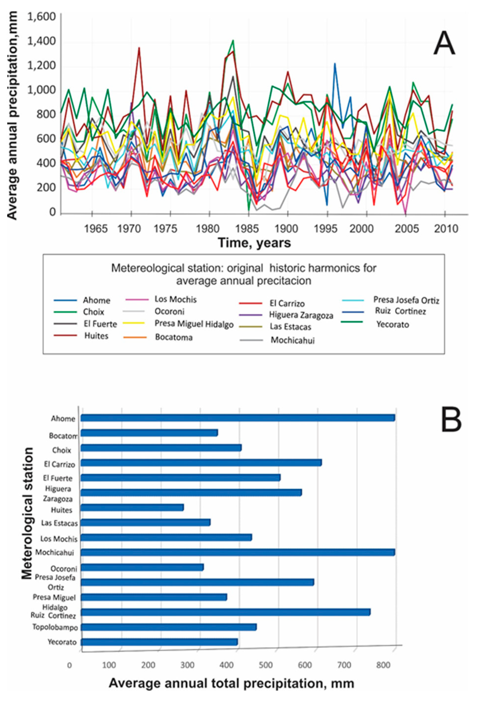
Within SMO, the station with the greatest magnitude corresponds to Yecorato, while the smallest, measuring 434.78 mm, is Las Estacas. Similarly, in the vicinity of SMO, the three largest catchments in mm were recorded, with an average total of = 811.22, 809.45, and 737.28, respectively for the stations of Yecorato, Huites, and Choix. Conversely, stations with smaller magnitudes, measuring in mm at = 260.99, 311.68, and 371.421, are identified respectively at the stations of Mochicahui, Higuera de Zaragoza, and El Carrizo in the coastal plain.
The graph in part A of Figure 2 represents the temporal variation of the original 16 St, constructed to conduct one-dimensional analysis on the behavior of . This analysis revealed irregularities; for instance, in 1986, an anomalous magnitude of = 258.59 mm, the lowest annual average within all 765 nominal values (m = 15, n = 51), was observed. The behavior continued with high annual values was characterized across the 1980s: 1980 (641.11 mm), 1982 (640.24 mm), 1983 (760.42 mm), and 1989 (639.20 mm). While the 1990s showed an irregular trend, with biannual minimum values in mm of as follows: 1994 (345.42 mm), 1996 (344.38 mm), and 1998 (364.20 mm). At the beginning of the 20th century, in 2003, an isolated and sporadic magnitude of = 671.30 mm was observed.
To classify the anomaly of 2003, considering the range R = [760.42, 288.50] corresponding to the maximum and minimum accumulated annual variation of in the area, it was deemed a medium to high rainfall event. This year marked the highest rainfall in the first decade of the twentieth century. If this outlier is disregarded, magnitudes fall within the range R = [376.90, 431.16], revolving around the value = 495.89 mm. The behavior of this first decade of 20th century presents cyclical behaviors of maximums and minimums in mm, exhibited in 2001 ( = (373.90 mm), 2002 ( = 440.18 mm), 2004 ( = 389.14 mm), 2009 ( = 392.19 mm), and 2010 ( = 431.16 mm) mm.
The Table 1 presents the results of individual statistical diagnosis applied to the original 16 datasets. The indictor punctual parameters of central tendency for min presented a range variation from 10.01 to 506.90 mm and max from 1417.60 to 551.50 mm, for from 811.22 to 261.00 mm, and from 8816.10 to 264.18 mm. The Statistical dispersion parameters showed Rabs values from 1417.60 to 551.50, σ from 228.42 to 109.37, σ2 m from 52174.74 to 11962.57, a CV range from 51.53 to 16.62, R2 from 0.11 to 2x10⁻³, and R from 0.17 to 0.52. The variation of asymmetry and shoring statistical parameters respectively present the following magnitudes: Skew_ from 1.63 to -0.16 and Kurt_ from 5.53 to -0.90. Finally, the positional statistical parameter for percentile 25% values ranges from 714.80 to 193.90 and for percentile 75% from 945.01 to 314.30.
Cconsidering respect to Ahome meteorological station an accumulated by individual variation of R = 0.45 in shared information among the others 15 St, there are high correlation in the information, indistinctively that all Sts displaying undefined trends in some positive and in others negative moments (Figure 2). This high correlation suggests a potential AC within the St, which could impact the spectral analysis of with signals from seasonal statistical processes.
For spectral analysis, it was considered preferable to work with seasonal stochastic processes due to their simpler and more stable statistical properties compared to non-seasonal processes. Non-seasonal processes can be more complex, as they may have AC over time, compromising results and introducing uncertainty and deviation from reality if not considered during the verification of seasonality assumptions.
The evolution of nominal values over time in a multiple analysis of for all meteorological stations exhibits a consistent behavior around the constant level = 504.53, with permanent changes dispersed in a joint variability. Indicated by the values of σ = 134.36 and σ2 = 18, 052.72 = 18,052.72. The result R2 = 0.21 respect to Ahome meteorological station suggests that they share 21% of their information, the distribution of nominal values more or less is converging at the same point measure of = 487.71, their asymmetry, defined by Skew_ = 0.453; indicate a slight positive concentration of nominee values slightly elongated to the right, while Kurt_ = 2.17 indicates a curve characterized by a normal or platicurve behavior.
The individual diagnosis and multiple analyses statistic of St are indicating a high level of shared information, both suggesting a potential AC within the St that may impact the spectral analysis of with signals from non-seasonal statistical processes.
Given that working with seasonal stochastic processes is more straightforward due to their simpler and more stable statistical properties compared to non-seasonal processes, which can be complex and varied; and considering the possible AC within the time series that could invalidate results, leading to uncertainty and deviation from reality, it became imperative to eradicate the level of AC in each St for verify the assumptions of seasonality in the information.
The following are the results of four statistical techniques used to analyze AC conditions. These results correspond to respective algorithms detecting AC within the St. It's important to remember that the presence of AC would invalidate any seasonality condition. The results of the first statistical tool to detect AC are presented in Table 2 and correspond to a low shared variance response of Ahome station compared to the rest of the St, making this station the dependent variable. R2 values range from 0 to 1, suggesting 100% similarity of information. A 21% correlation with R2 was considered possible with AC.
Contrasts [prob. (F_stat) vs. α], with values for prob. (F_statisitc) ranging from [0.8, 0.33], exceeded α < 0.05, indicating no significant differences between nominal values of in almost all 16 St. Prob. > 0.05 in the contrast [prob. (prob. (F_stat) vs. α] was associated with stations presenting the greatest strength in the absence of correlation (greater difference in shared information). The stations that exhibited the greatest strength in the absence of correlation (indicating greater difference in shared information) include Bocatoma Prob. = 0.74), Choix (prob. = 0.60), El Fuerte (prob. = 0.84), Las Estacas (prob. = 0.71), Ocoroni (prob. = 0.81), Presa Josefa Ortiz (Prob. = 0.79) and Yecorato (Prob. = 0.80).

Table 1.
Statistical analysis of 16 time series (1963-2011) for estimating central tendency, dispersion, asymmetry, and statistical bolstering in average annual precipitation in northwestern Mexico's mountainous zones and coastal plains.
Table 1.
Statistical analysis of 16 time series (1963-2011) for estimating central tendency, dispersion, asymmetry, and statistical bolstering in average annual precipitation in northwestern Mexico's mountainous zones and coastal plains.
| Higuera Zaragoza | Ahome | Los Mochis | Mochicahui | Bocatoma | Las Estacas | Presa Josefa Ortiz | El Fuerte | Presa Miguel Hidalgo | Yecorato | Choix | Huites | Ocoroni | El Carrizo | Topolo-bampo | Ruiz Cortines | |
| 87.10 | 68.20 | 10.00 | 26.60 | 180.00 | 152.00 | 209.60 | 338.20 | 276.80 | 506.90 | 27.40 | 418.50 | 264.50 | 127.30 | 69.50 | 164.00 | |
| 905.80 | 1228.40 | 683.70 | 551.50 | 737.10 | 724.20 | 895.20 | 1122.00 | 993.20 | 1042.50 | 1417.60 | 1357.40 | 821.00 | 729.50 | 953.00 | 797.90 | |
| 311.69 | 398.66 | 329.27 | 261.00 | 446.91 | 434.79 | 507.84 | 593.56 | 613.00 | 811.22 | 737.29 | 809.46 | 562.10 | 371.42 | 347.89 | 408.45 | |
| 282.30 | 365.00 | 328.80 | 264.18 | 421.60 | 431.99 | 500.76 | 581.50 | 580.10 | 816.10 | 733.70 | 805.43 | 556.57 | 383.10 | 341.12 | 375.60 | |
| Rabs | 905.80 | 1228.40 | 683.70 | 551.50 | 737.10 | 724.20 | 895.20 | 1122.00 | 993.20 | 1042.50 | 1417.60 | 1357.40 | 821.00 | 729.50 | 953.00 | 797.90 |
| σ | 138.83 | 205.44 | 144.59 | 112.78 | 147.77 | 109.99 | 127.54 | 153.47 | 153.21 | 134.84 | 228.42 | 213.40 | 109.37 | 120.08 | 159.95 | 147.22 |
| σ2 | 19273.46 | 42205.03 | 20906.51 | 12719.91 | 21835.74 | 12097.66 | 16265.9 | 23553.16 | 23472.22 | 18181.87 | 52174.74 | 45537.87 | 11962.57 | 14418.70 | 25585.30 | 21673.28 |
| CV | 818.70 | 1296.60 | 683.70 | 578.10 | 917.10 | 876.20 | 1104.80 | 1460.20 | 1270.00 | 1549.40 | 1445.00 | 1775.90 | 1085.50 | 856.80 | 1022.50 | 961.90 |
| R | 0.09 | 1.00 | 0.04 | 0.04 | 0.03 | 0.001 | 0.01 | 0.01 | 0.01 | 0.002 | 0.01 | 0.0002 | 0.00 | 0.11 | 0.03 | 0.05 |
| R2 | 0.45 | 0.52 | 0.44 | 0.43 | 0.33 | 0.25 | 0.25 | 0.26 | 0.25 | 0.17 | 0.31 | 0.26 | 0.19 | 0.32 | 0.46 | 0.36 |
| 1.63 | 1.61 | 0.34 | 0.06 | 0.23 | 0.24 | 0.65 | 1.16 | 0.34 | -0.12 | 0.10 | 0.43 | -0.16 | 0.34 | 0.96 | 0.85 | |
| 5.53 | 4.81 | -0.24 | 0.51 | -0.90 | 0.23 | 1.60 | 2.29 | -0.26 | -0.68 | 1.90 | 0.29 | 1.10 | 0.41 | 2.83 | 0.38 | |
| Q2 | 227.50 | 248.30 | 198.00 | 193.90 | 332.00 | 344.70 | 413.30 | 493.90 | 493.80 | 714.80 | 590.50 | 633.50 | 502.60 | 255.80 | 223.60 | 304.40 |
| Q3 | 367.80 | 496.27 | 430.20 | 314.30 | 576.80 | 531.90 | 568.80 | 669.20 | 746.00 | 908.70 | 894.10 | 945.00 | 619.81 | 443.87 | 438.40 | 469.10 |
| and = maximums and minimum limits in mm, = Arithmetic mean, = Median, Rabs = Absolute range, σ = standard deviation of the distribution, σ2 = variance of the distribution, CV = Coefficient of variation, R = Coefficient of dispersion, R2 = Coefficient of correlation, Coefficient of asymmetry, = Ccoefficient of kurtosis, Q2 = percentile 25th and Q3 = percentile 75th. | ||||||||||||||||
The counterpart of R2, namely k2 = 1 − R2 (coefficient of alienation or indeterminacy), demonstrated incidences between the nominal comparatives and the total proportion of σ2, attributing 79% of the information to no correlation. This suggests the possibility of AC within any St. The RLM result of 21% of R2 hinted at potential disturbances within the St, hindering its representation as a stationary stochastic process. Consequently, the hypothesis Ho was rejected initially, and the alternative H1 was accepted.
(t _stat_DW)
Table 2.
Multiple Linear Regression (MLR) of 16 historical series concerning shared variance in average annual precipitation with Ahome station on the coastal plains and mountain zones of northwestern Mexico.
Table 2.
Multiple Linear Regression (MLR) of 16 historical series concerning shared variance in average annual precipitation with Ahome station on the coastal plains and mountain zones of northwestern Mexico.
| Dependent Variable: AHOME Method: Least Squares Ordinary | ||||
| Sample: 1961 2011 Included observations: 51 | ||||
| Variable | Coefficient | Std. Error | t-Statistic | Prob. |
| C | 281.077 | 283.589 | 0.991 | 0.328 |
| Bocatoma | 0.132 | 0.388 | 0.339 | 0.736 |
| Choix | 0.129 | 0.244 | 0.528 | 0.601 |
| El Carrizo | 0.462 | 0.375 | 1.231 | 0.227 |
| El Fuerte | -0.086 | 0.435 | -0.198 | 0.844 |
| Higuera Zaragoza | 0.349 | 0.410 | 0.852 | 0.400 |
| Huites | -0.134 | 0.239 | -0.560 | 0.579 |
| Las Estacas | -0.175 | 0.461 | -0.380 | 0.707 |
| Los Mochis | -0.301 | 0.488 | -0.616 | 0.542 |
| Mochicahui | 0.325 | 0.377 | 0.861 | 0.395 |
| Ocoroni | -0.011 | 0.301 | -0.036 | 0.972 |
| Presa Josefa Ortiz | 0.123 | 0.466 | 0.264 | 0.793 |
| Presa Miguel Hidalgo | -0.353 | 0.423 | -0.835 | 0.409 |
| Ruiz Cortines | 0.234 | 0.362 | 0.646 | 0.522 |
| Topolobampo | 0.174 | 0.297 | 0.587 | 0.561 |
| Yecorato | -0.078 | 0.303 | -0.258 | 0.798 |
| R2 | 0.21 | Mean dependent var | 398.658 | |
| Adjusted R2 | -0.12 | S.D. dependent var | 205.439 | |
| S.E. of regression | 217.73 | Akaike info criterion | 13.855 | |
| Sum squared resid | 1,659,201 | Schwarz criterion | 14.461 | |
| Log likelihood | -337.31 | Hannan-Quinn criterion. | 14.087 | |
| F-statistic | 0.63 | Durbin-Watson stat | 1.717 | |
| (t_stat_DW) | ||||
Direct detection of AC using contrasts ([prob. (F_statisitc) vs. α) between the probabilities of F_statisitc and the significance level 0.05 serves as a partial indicator of AC. However, the methodology's uncertainties regarding specification errors led to hesitation in assuming the absence of AC. The RLM method alone did not offer sufficient guarantees to conclusively argue against AC in the models analyzed.
Hence, three statistical tools were employed to visually identify areas where AC might occur. The second method examined the spatial distribution of variation in similarity, illustrating the 21% information concentration. It also identified AC by comparing signals along a linear distribution, visually represented at the scaleogram's base. While both the RLM and MSC using R2 for analysis, the latter detects areas of AC, as depicted in Figure 3. The red vertex of the triangle highlights the high similarity between the first and last values of the matrix m x n. Similarly, the base of the triangle in the same color indicates comparison pairs showing similarity.
Although the RLM initially suggested absence of AC (Table I), the MSC reveals AC within the information previously assumed free of AC. This new insight offers a more comprehensive understanding, discouraging reliance solely on contrast tests for analyzing seasonality assumptions in the St.
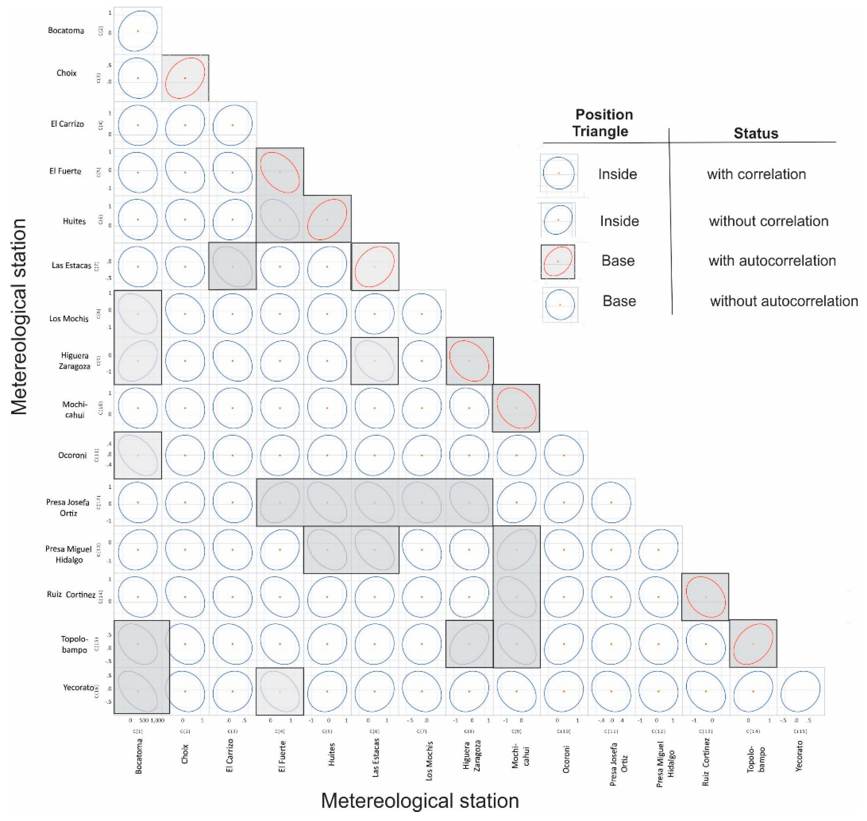
To identify the St potentially affected by the outlier AC effect and to ensure accurate data representation with series of seasonal stochastic processes, the third method GCE was employed and the results are depicted in Figure 4. Figure 4 still within the triangle indicate stations that didn't exhibit AC or correlation, meaning they didn't share their σ2 with another St or within themselves. Conversely, the figures in red within the triangle show stations displaying AC when their information is compared. Additionally, stations with no correlation when compared with each other are indicated within the triangle. Out of the 120 geometric figures formed by the contrasts, 28 tended to form an ellipse, indicating 23.33% shared information. This result closely aligns with that of the RLM (R2 = 0.21).
Among the 92 ellipses with geometric shapes tending not to form an exact ellipse but rather circles, these contrasts are exempt from correlation and AC. Specifically, the ellipses enclosed in a rectangle and marked in red in Figure 4 indicated AC when compared with themselves through this method. The tendency to form ellipses, showed the next eight datasets with presence of AC: Choix, El Fuerte, Higuera Zaragoza, Huites, Los Mochis, Mochicahui, Ruiz Cortines, and Topolobampo.
The GCE analysis revealed that 50% of the St did not exhibit AC, while the remaining 50% required adjustment to achieve stationarity.
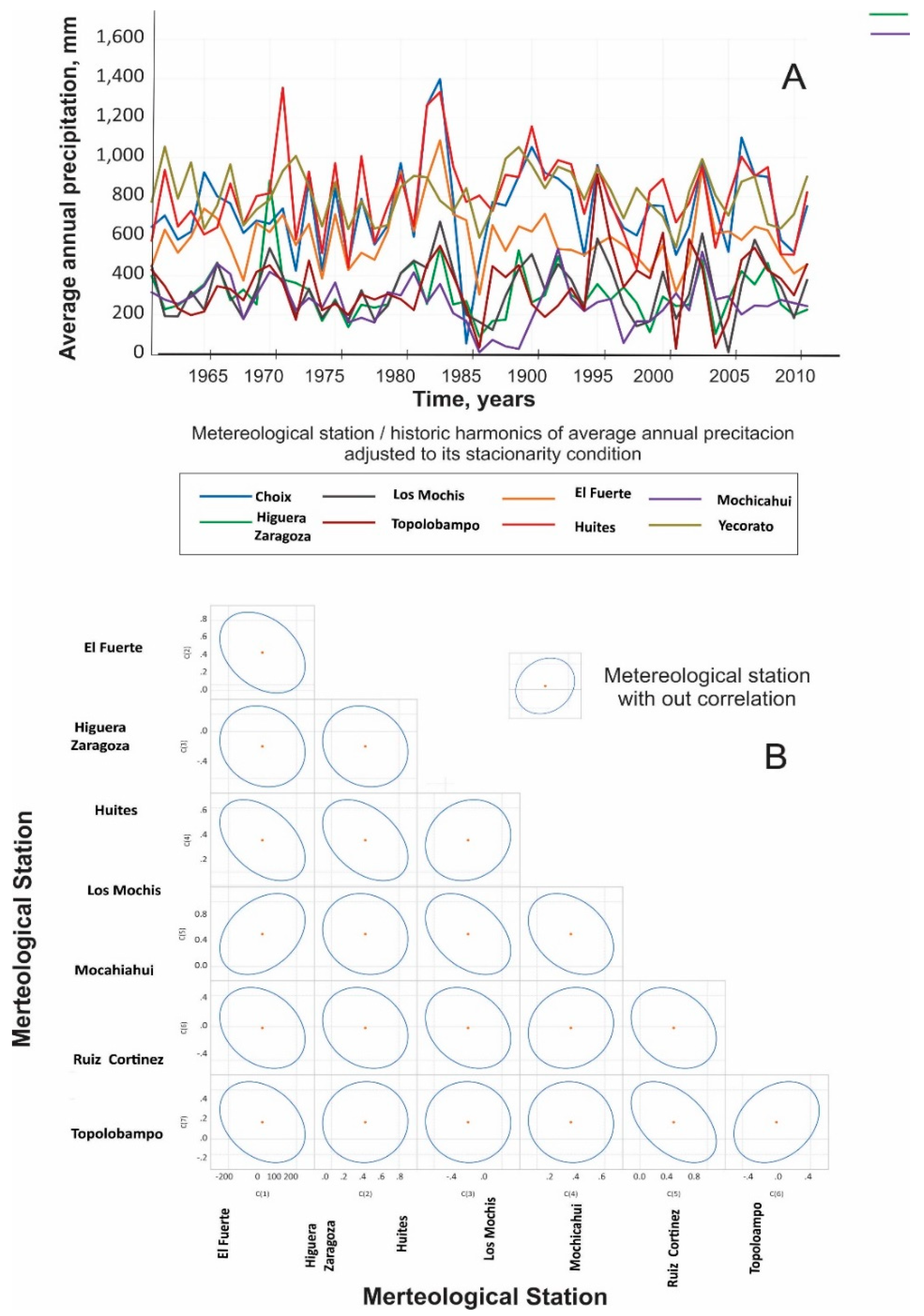
The random effects detected in GCE analysis in the dataset were found to deviate from the actual conditions observed in rainfall patterns. To address this, it was necessary to process the dataset of these 8 St using the STL-Decomposition method.
For verify if the AC was reduced, the eight St underwent adjustment, again were retested using GCE and t-stat-VIF methods. Figure 5, part A, displays the graphical representation of the adjusted 8 St with STL-Decomposition is displayed, while Part B confirms the reduced AC indicated by the change from ellipses tending to form circles. With this reduction in effect, a new RLM was conducted. The new results of R2 = 0.12 and R2 adjusted = - 0.26 reported on Table 3, were considered acceptable, thereby increasing confidence in the reduction of AC within the St. This reduction allowed for the application of the t_stat_DFA contrast to verify the seasonality condition within the dataset.
Table 3.
Multiple linear regression of 15 historical series concerning Ocoroni station (high initial correlation (Prob. = 0.972)), once 50% of non-stationary series were adjusted by STL-Descomposition to their respective stationary behavior.
Table 3.
Multiple linear regression of 15 historical series concerning Ocoroni station (high initial correlation (Prob. = 0.972)), once 50% of non-stationary series were adjusted by STL-Descomposition to their respective stationary behavior.
| Dependent Variable: AHOME Method: Least Squares | ||||
| Sample: 1961 2011 Included observations: 51 | ||||
| Variable | Coefficient | Std. Error | t-Statistic | Prob. |
| C | 428.8138 | 144.6235 | 2.965034 | 0.0054 |
| Ahome | -0.00021 | 0.096291 | -0.002179 | 0.9983 |
| Bocatoma | -0.015362 | 0.224837 | -0.068326 | 0.9459 |
| Choix | -0.007158 | 0.136069 | -0.052603 | 0.9583 |
| El Carrizo | -0.138392 | 0.210574 | -0.657214 | 0.5153 |
| El Fuerte | -0.087261 | 0.241085 | -0.36195 | 0.7196 |
| Higuera Zaragoza | -0.138028 | 0.238347 | -0.579105 | 0.5662 |
| Huites | -0.08107 | 0.132405 | -0.61229 | 0.5443 |
| Las Estacas | 0.003729 | 0.262262 | 0.014218 | 0.9887 |
| Los Mochis | -0.11531 | 0.288566 | -0.399596 | 0.6919 |
| Mochicahui | 0.185702 | 0.222917 | 0.833055 | 0.4105 |
| Presa Josefa Ortiz | 0.081122 | 0.257958 | 0.314479 | 0.755 |
| Presa Miguel Hidalgo | 0.089051 | 0.242068 | 0.367875 | 0.7152 |
| Ruiz Cortines | 0.214074 | 0.213303 | 1.003612 | 0.3225 |
| Topolobampo | -0.003981 | 0.172051 | -0.023137 | 0.9817 |
| Yecorato | 0.201397 | 0.1634 | 1.23254 | 0.226 |
| R2 | 0.12 | Mean dependent var | 562.104 | |
| Adjusted R2 | -0.26 | S.D. dependent var | 109.374 | |
| S.E. of regression | 122.67 | Akaike info criterion | 12.708 | |
| Sum squared resid | 526,687 | Schwarz criterion | 13.314 | |
| Log likelihood | -308.05 | Hannan-Quinn criter. | 12.939 | |
| F-statistic | 0.32 | Durbin-Watson stat | 1.893 | |
| Prob(F-statistic) | 0.99 | (t_stat_DW) | ||
Figure 4.
Algorithm correlating ellipses, in red marking geometric shapes at the triangle's base indicating a tendency for ellipses associated with harmonic autocorrelation.
Figure 4.
Algorithm correlating ellipses, in red marking geometric shapes at the triangle's base indicating a tendency for ellipses associated with harmonic autocorrelation.
Note that the results in Table 2 and Table 3 highlight differences between the results obtained for the F_stat and Prob(F_stat) statistics in the original 16 datasets and the new results after adjusting the 8 Sts to achieve stationarity. These adjusted datasets were then reintroduced to obtain the second RLM shown in Table 3. The first RLM in Table 1 presents values of F_stat = 0.63, Prob(F_stat) = 0.82, and R2 = 0.21. In contrast, the second RLM in Table 3 shows these magnitudes distributed as follows: F_stat = 0.34, Prob(F_stat) = 0.98, and R2 = 0.11. It is evident that there was a reduction after adjusting for seasonality using the STL-Decomposition technique.
The results of t_stat_FIV are displayed in Table 4, where the third column facilitates the establishment of the contrast [t_stat_FIV vs. VIF < 10]. It's notable that all values in this column fall within the range R = [1.3, 5.71], indicating that the magnitudes of t_stat_FIV are consistently < 10. Consequently, these findings suggest a complete absence of heteroskedasticity and correlation, effectively dismissing the potential presence of AC in the representation of .
Figure 5.
(A) displays the graphical representation of the adjusted 8 St with STL-Descomposition, and (B) confirms the reduced AC indicated by the change from ellipses tending to form circles.
Figure 5.
(A) displays the graphical representation of the adjusted 8 St with STL-Descomposition, and (B) confirms the reduced AC indicated by the change from ellipses tending to form circles.
This new condition on dataset prepares the ground for applying t_stat_DFA to ascertain the presence of seasonality in each St, employing a 5% level of critical values set at -3.5 for comparison with t_stat_DFA. This method offers full confidence in determining the presence or absence of seasonality, allowing us to either accept or reject the hypothesis “H0 = has a unit root exogenous," and depending on its presence or absence, decide regarding the definition of stationarity accept or reject the hypothesis “H0 = has a unit root exogenous: constant and linear trend”, whether the datasets of are stationary or non-stationary.
Table 4.
Results of t_stat_FIV in 16 datasets of historical series, using the significance level VIF < 10 associated with the maximum value to search a multicollinearity in respective nominal factors.
Table 4.
Results of t_stat_FIV in 16 datasets of historical series, using the significance level VIF < 10 associated with the maximum value to search a multicollinearity in respective nominal factors.
| jfigure | Coefficient Variance | Uncentered VIF | Centered VIF |
| 20915.97 | 70.89 | NA | |
| Ahome | 0.01 | 6.29 | 1.30 |
| Bocatoma | 0.05 | 37.89 | 3.67 |
| Choix | 0.02 | 37.15 | 3.10 |
| El Carrizo | 0.04 | 22.86 | 2.12 |
| El Fuerte | 0.06 | 73.86 | 4.46 |
| Higuera Zaragoza | 0.06 | 22.12 | 3.41 |
| Huites | 0.02 | 41.50 | 2.59 |
| Las Estacas | 0.07 | 46.83 | 2.76 |
| Los Mochis | 0.08 | 36.26 | 5.72 |
| Mochicahui | 0.05 | 13.56 | 2.09 |
| Presa Josefa Ortiz | 0.07 | 61.76 | 3.60 |
| Presa Miguel Hidalgo | 0.06 | 79.19 | 4.57 |
| Ruiz Cortines | 0.05 | 28.99 | 3.28 |
| Topolobampo | 0.03 | 14.63 | 2.49 |
| Yecorato | 0.03 | 61.16 | 1.61 |
The Outliers have been identified and corrected. Consequently, the following section will present the results verifying seasonality in the Sts using t_Stat_DFA to accept or reject the Ho hypothesis regarding the presence or absence of I(1), associated respectively with seasonality or non-seasonality in any St. The results of the t_Stat_DFA contrasts are displayed in Table 5. This diagnosis reflects the outcomes obtained after all 16 series passed graphical inspection and demonstrated the absence of AC.
The Table 5 show results of t_Stat_DFA obtained applying this test in its simple original manifestation and including those that were corrected by STL_Desomposition and the St themselves presented free of any process in their seasonal form, that is, all tests were performed considering as a dependent variable the first difference of , and given that, the Sts showed different positive or negative trends with respect to time, that is, without a tendency defined by a specific value around which each cloud of values was distributed; It was considered reasonable in the face of this behavior to perform the I of t_Stat_DFA without the existence of a slope. The analysis also considered the nature of positive values of the measurement with values above zero () in such a way that they did not manifest interception with the axis of the direction xi. This behavior in its seasonal form of the St allowed to select from the three forms that exist to perform the of t_Stat_DFA to analysis in levels without tendency and without intercept to leave aside the contrasts Stat_DFA in first and second differentiation. Within this test also for contrasts to again the possible existence of an AC in the information through the use of a Lag = 10 selected automatically in Eview 12.0 to compensate for this condition.
Before proceeding to accept or reject the Ho hypothesis of seasonality with the contrast of the results of t_stat_DFA and the critical significance level of 5% equivalent to -3.5, it was first verified whether the value of t_stat_DW was included among the established limits of the range R = [1.85, 2.15]; and due to it was founded ion limits established, then with all certainty was affirmed that an AC in the model not was present and also it was indicator that the algorithms applied for the detection of non-seasonality together with the adjustments criteria had the expected results.
To this moment the datasets of 16 Sts, are results based of t_stat_DW, t_stat_DFA, and p_values and indicated absence of AC within these models. Parallelly the t_stat_DFA values respect to the critical level of significance of -3.5, also confirmed the rejection of the Ho hypothesis for seasonality in all 16 St datasets, as all t_stat_DFA values fell within the rejection zone (beyond the critical level of significance of -3.5), the results suggest that the St datasets, along with their autoregressive representations, did not display tendencies towards or equal to I(1), affirming so their stochastic behavior with seasonal tendencies.
Additionally, the P_value variations ranging from 0.0001 to 0.004 further supported the verification of seasonality within the St datasets. These contrasts provided high confidence levels in rejecting the Ho hypothesis, with the errors in rejecting Ho being lower than the accepted error level of 5%.
With the absence of AC established within the models, the nominal values of the 16 St exhibited consistent behaviors around specific values of and σ2 = K. This assurance of stochastic, stationary, constant, and stable behaviors within these datasets facilitated the application of processes and algorithms, culminating in the determination of from 1961 to 2011 within each meteorological station. The spatial variation mentioned, is shown in part A of Figure 6, represents the average sum of the 51 nominee values for each dataset the datasets were transformed to the frequency domain to derive and further analyzed through radial integration to ascertain /. The statistical results obtained before transforming into frequency domains and applying similar tools used for AC and seasonality verification on the 16 St are depicted in Table 5, indicating the rejection of the Ho hypothesis of seasonality and affirming the presence of seasonality in .
The final verification of the seasonality condition in ensured that only stationary processes were employed throughout the study period, offering certainty regarding the spatial variability behavior and the gravity zoning effects caused by variable rain power in the study area, especially during the crucial initial 30 minutes where the most significant rainfall magnitudes occur, impacting the internal soil structure.
The results of t-stat_DFA analysis for are showing on Table 6 and reveals that the t_stat_DW = 1.99 within the range previously seting as R = [1.85, 2.15], indicating the absence of AC in the model. Similarly, the t_stat_DFA = -5.69 compared with NC5% = -3.06 signifies the acceptance zone, suggesting an absence of I(1) in the characteristic equation for both the original data and its first autoregressive representation. Consequently, was determined to be a stationary stochastic process represented by 504.53 mm and 18,052.72 mm for their variance.
Table 6.
Statistic test Durvin Watson (t_stat_DW) and Augmented Dickey-Fuller test (t_stat_DFA) showing respectively the absence of autocorrelation and the presence of seasonality in the historical series of total annual average precipitation in the coastal plain and mountain zone of northwestern Sinaloa, Mexico.
| Augmented Dickey-Fuller Unit Root Test on PRECIP | ||||
| Null Hypothesis: PRECIP has a unit root Exogenous: Constant, Linear Trend Lag Length: 0 (Automatic - based on SIC, maxlag = 10) | ||||
| t-stat_DFA | Prob.* | |||
| Augmented Dickey- Fuller test statistic | -5.694 | 0.0001 | ||
| Test critical values | 1% level | -4.152511 | ||
| 5% level | -3.502373 | |||
| % level | -3.180699 | |||
| *MacKinnon (1996) one-sided p-values. | ||||
| Augmented Dickey-Fuller Test Equation | ||||
| Dependent Variable: D(PRECIP) | ||||
| Method: Least Squares | ||||
| Sample (adjusted): 1962 2011 | ||||
| Included observations: 50 after adjustments | ||||
| Variable | Coefficient | Std. Error | t-Statistic | Prob. |
| PRECIP(-1) | -0.817 | 0.143 | -5.695 | 0.000 |
| C | 390.143 | 73.160 | 5.333 | 0.000 |
| @TREND("1961") | -0.021 | 0.887 | -0.023 | 0.982 |
| R2 | 0.408 | Mean dependent var | -0.104 | |
| Adjusted R2 | 0.383 | S.D. dependent var | 115.259 | |
| S.E. of regression | 90.527 | Akaike info criterion | 11.907 | |
| Sum squared resid | 385175.000 | Schwarz criterion | 12.022 | |
| Log likelihood | -294.683 | Hannan-Quinn criter. | 11.951 | |
| F-statistic | 16.215 | Durbin-Watson stat | 1.996 | |
| Prob(F-statistic) | 0.000 | (t_stat_DW) | ||
Post-transformation of domains using FFT, the real shape of // in the study area was understood, along with the intensity of the initial impulses representing the spectral power of rain in different regions.
The spatial variability of the magnitude of the first impulses, represented in part B of Figure 6, illustrated a non-random pattern. Figure 6 portrays the graphical representation of // along with the Neperian logarithms of // in relation to spatial frequency or wavenumber. The behavior of /(r)/ curves primary displays an exponential fall, with distinguishable linear relations between frequency ranges and their respective amplitudes. The exponential decay towards linear trends intensifies with increasing wavenumbers and potentially correlates with events of lower intensity originating from local sources.
Figure 6 presents a graphical representation of cycles per unit of distance, illustrating /(r)/ in terms of frequency and showcasing the magnitude of initial impulses, providing insights into the spectral power of rain.
These visualizations facilitate the comprehension of average total rainfall intensity at each meteorological station in relation to the logarithm of [//]/4 π. Hhighlights distinct patterns of /(r)/ and its exponential decay across different stations. Moreover, the analysis of first impulses reveals unique magnitudes and frequency variations, with a notable concentration at 0.06 cycles/mm. Each meteorological station exhibits distinct behaviors in terms of rainfall intensity and frequency decay. Notably, the mesh of meteorological stations displays atypical power density behavior, indicating sequential and gradual changes in intensity related to local phenomena of lower intensity within its coverage area.
Figure 7, part A, illustrates the spatial variability of revealing low accumulated historical rainfall at the Las Estacas meteorological station. This water deficiency poses a risk of water stress in this agriculturally significant area. However, for the same zone, despite the low accumulation, the rain intensity during the initial minutes suggests intermediate values, indicating potentially less damage to soil compared to “The Agricultural Heart of Mexico”, which experiences more substantial absence of rainfall. Additionally, the El Carrizo meteorological station exhibits a gradual exponential decrease in rain frequency, which may affect surrounding regions with higher rainfall, potentially diminishing their influence.
Figure 6.
Radial potential spectrum depicts 16 historical stationary series of average annual total precipitation (mm), showcasing the magnitudes of initial impulses associated with moments of peak rainfall risk within the "Río Fuerte" and "Río Sinaloa" hydrographic and agricultural basins.
Figure 6.
Radial potential spectrum depicts 16 historical stationary series of average annual total precipitation (mm), showcasing the magnitudes of initial impulses associated with moments of peak rainfall risk within the "Río Fuerte" and "Río Sinaloa" hydrographic and agricultural basins.
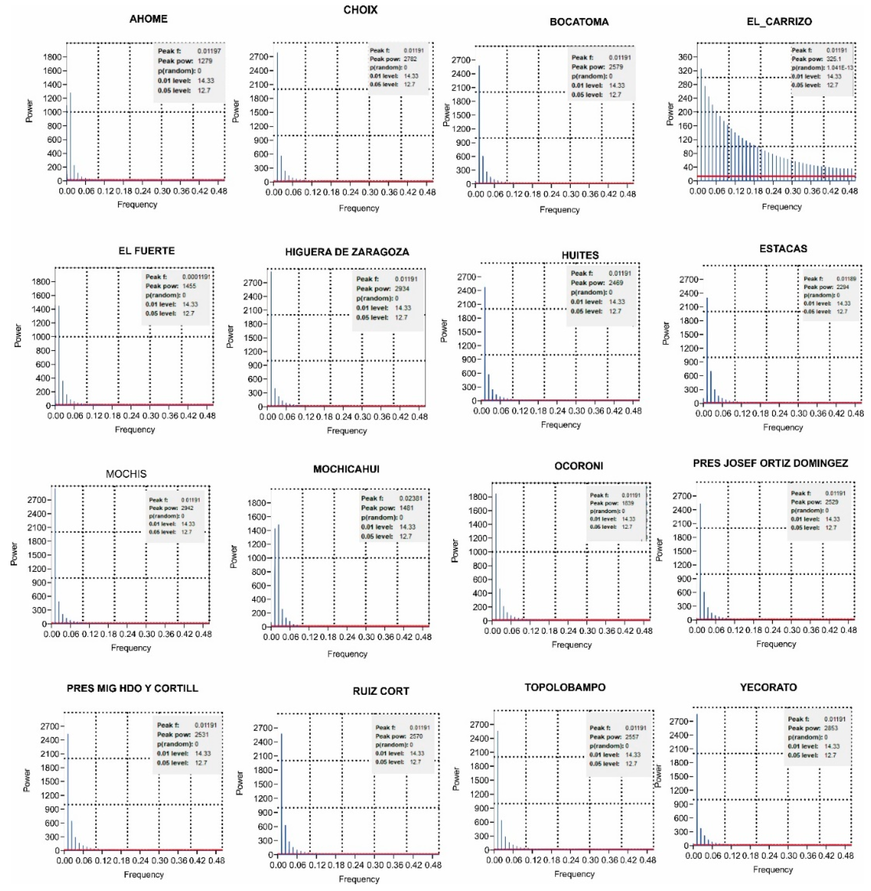
In the northern and central zones, there is noticeable variation in rainfall intensity, with maximum values ranging from 620 to 800 mm. Conversely, areas near the Sinaloa River mouth and the Sea of Cortez exhibit minimal rainfall magnitudes, ranging from 240 to 360 mm. While these minimal magnitudes support agricultural activities, they can also lead to water deficits and impact soil conditions due to high evapotranspiration rates compared to local water beginning by precipitation and groundwater flow.
This spatial variation in rainfall intensity and its initial impulses /(r)/ across maps in Figure 7 are attributed to variable microclimates affecting meteorological factors, generating convective precipitation typical of warm latitudes. Variability in atmospheric pressure, temperature, and humidity within these microclimates contributes to the diverse patterns observed during the initial moments of rainfall, crucial for understanding how rain impacts the granulometric structure of the soil.
Analysis underscores the varying consequences and severity of rain's effects on soil structure, particularly during the initial moments of rainfall, which pose a risk to soil integrity. Different microclimates across the study area significantly impact the severity of consequences resulting from rainfall power, particularly in the first 7 to 30 minutes, crucial for assessing soil degradation risks.
The is risk is more pronounced in mountainous areas and the central zone parallel to the Sea of Cortez. It highlights the potential for accelerated degradation of agricultural soils due to water deficit and structural changes caused by rainfall.
Figure 7.
(A) Spatial variability (mm) of average annual total precipitation: equipotential curves (620-800 mm), and (B) magnitudes variations of initial impulses showing severe moments of soil degradation due to rainfall.
Figure 7.
(A) Spatial variability (mm) of average annual total precipitation: equipotential curves (620-800 mm), and (B) magnitudes variations of initial impulses showing severe moments of soil degradation due to rainfall.
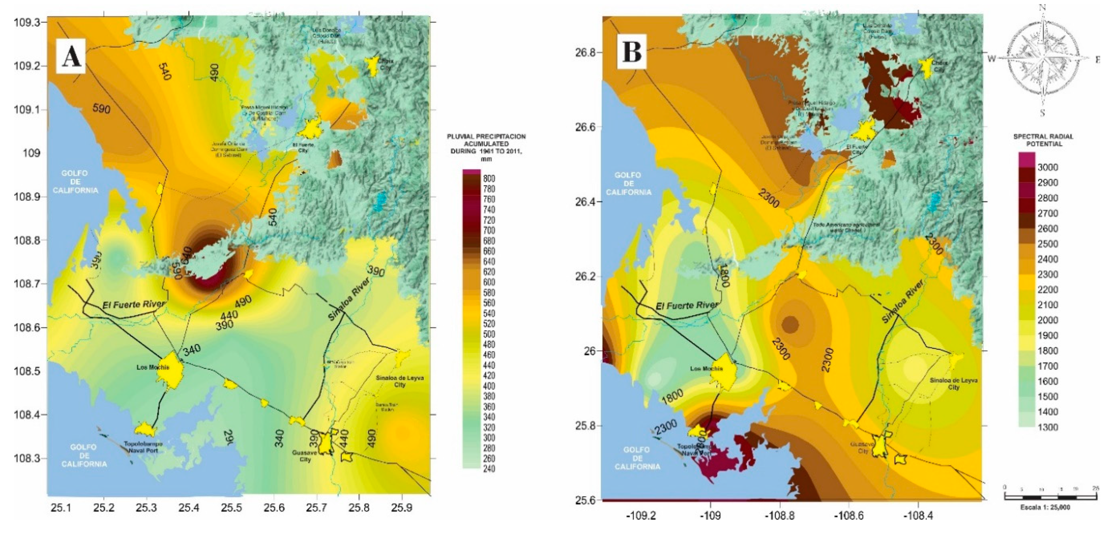
These severe consequences are not limited to “The Agricultural Heart of Mexico” but also extend along the coastal regions, demanding urgent attention for soil restoration, considering the implications of climate change and globalization demands.
Figure 8 illustrates the severity levels of consequences from the initial minutes of /(r)/. Over time, the highest severity levels extend across coastal areas, potentially accelerating land degradation. Three categories of severity with variable impacts on soil were identified:
Moderate Consequences: These areas demand immediate conservation actions to mitigate the impacts, as the consequences will persist and require significant effort for restoration.
Important Consequences: This severity category requires detailed studies to understand the current soil conditions. Immediate actions are needed to stabilize the soil structure and regulate its properties, considering porosity, water retention capacity, and organic matter development.
Catastrophic Effects: These areas have sustained severe damage and exploitation without proper consideration. They're currently unsuitable for sustainable agriculture and necessitate exhaustive recovery efforts for long-term restoration due to their difficult recovery state.
The classification of severity helps identify regions that need urgent attention for conservation, areas requiring comprehensive studies for stabilization, and those that demand long-term recovery strategies due to their current unsustainable state.
Figure 8.
Classification of levels of severity of consequences (dimensionless) on soil face to effects produced by the rainfall, situation that could produce accelerations to it degradation.
Figure 8.
Classification of levels of severity of consequences (dimensionless) on soil face to effects produced by the rainfall, situation that could produce accelerations to it degradation.
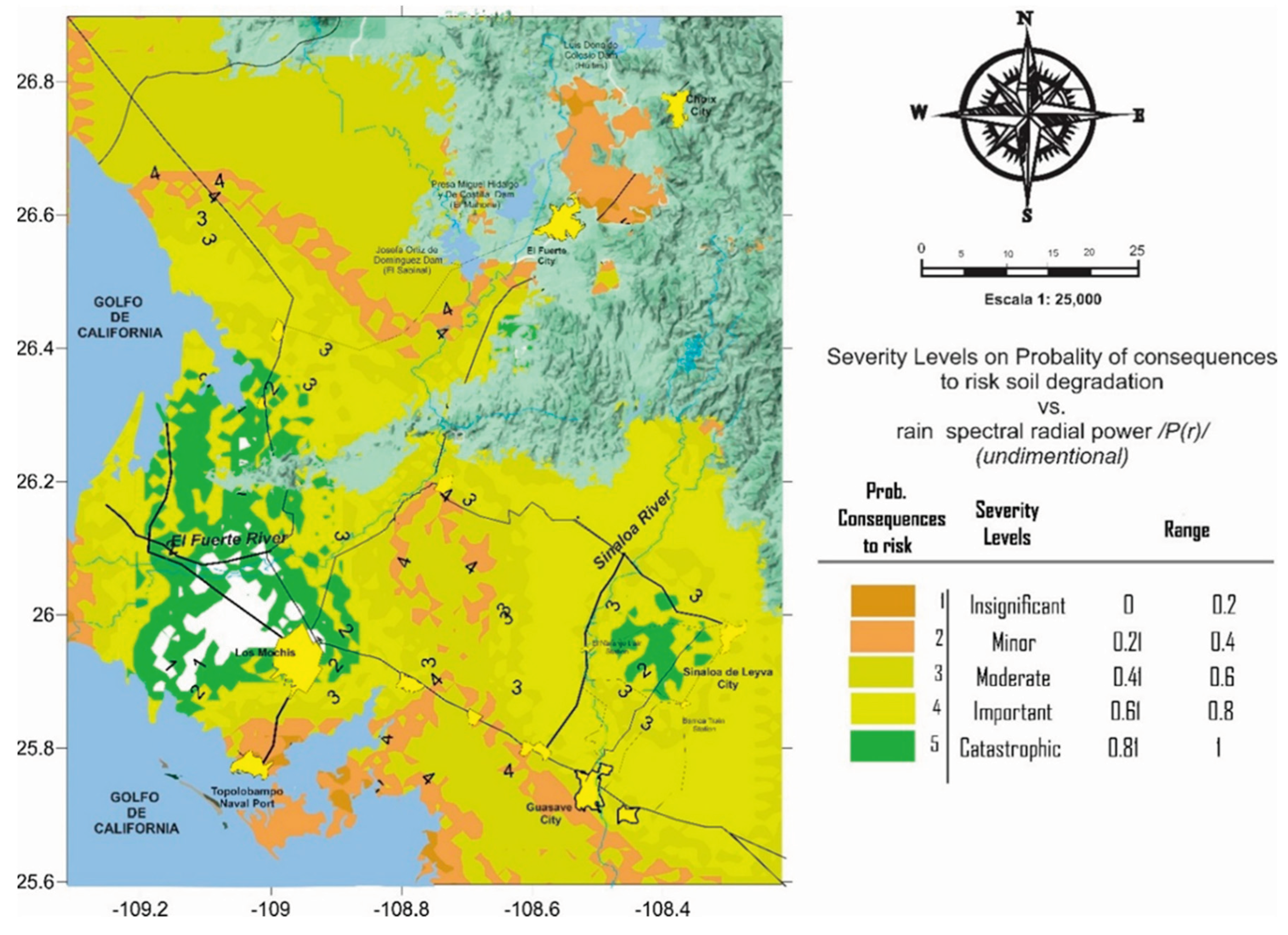
4. Discussion
The information gathered constitutes a comprehensive database and methodology that employs a suite of contemporary statistical tools. These tools are applied to generate crucial insights for the development of management plans aimed at risk mitigation based on the severity of consequences resulting from rainfall, a pivotal factor influencing soil structural degradation. This information also holds potential utility for future research endeavors, territorial planning initiatives, and various governmental or private projects focused on conserving agricultural soil in the region.
Presently, the region, comprised of the key valleys in northwester Mexico, lacks adequate recognition in the international agricultural market. The environmental value of its goods and services is not duly acknowledged, leading to a disparity in fair representation. This oversight is particularly concerning given the historical damage inflicted on the soil, directly impacting productivity across the agricultural cycle from planting to distribution.
Neglecting the genuine cost of agricultural products within the value chain creates a market failure, negatively impacting overall costs and, subsequently, the economy and welfare of the population Mexico [37]. The adverse effects of climate change on various global agricultural systems, exacerbated by a 1.1°C increase in average temperature, further underscore the urgency of addressing environmental issues in Mexico [38].
The changes in environmental components due to climate change in the region's valleys, as indicated by the historical , may contribute to accelerated soil cultural degradation. This situation could jeopardize “The Agricultural Heart of Mexico”, potentially affecting crop physiological processes, growth, and overall production.
To address these challenges, the region requires immediate optimization of both surface and underground water resources. Water deficit, aggravated by the arid and semi-arid climate and climatic instabilities, poses a significant threat to sustainable agriculture [38]. The findings highlight a water deficit persisting for decades, impacting soil structural arrangement and emphasizing the need for continued research.
To ensure sustainable agriculture in the region, a shift towards water-efficient crops is imperative. Studies focusing on crops with a balance in water management, emphasizing productivity efficiency, are crucial for adapting to the limited water environment [39]. The detected changes in the soil structure demand a commitment to repairing the damage caused and identifying the associated risks and consequences, categorizing them based on severity.
Quantifying GHG emissions associated with food production is essential for addressing climate change impacts and responses to climate change acording at its: opportunities and barriers in fazce to found a new adaptation [40]. The valuation of environmental assets, including soil resources, must become a priority in sustainable development, attributing fair environmental values based on soil characteristics. Agricultural sustainability necessitates a restructuring of natural resource management and parallel routes to international trade openness.
In this era of modern globalization, Mexican agriculture must strive for sustainability. Achieving this goal involves restructuring natural resource management and adopting parallel strategies for international trade openness. The impacts of human and natural activities altering the particle size structure of the soil must be considered in management plans for the correct and sustainable utilization of natural resources.
Assigning fair environmental values to agricultural assets, with indicators designed based on land use, GHG emissions, risk, and current vulnerability, is crucial. This is particularly relevant in the case of rainfall, a sensitive phenomenon to climate change. The information generated in this study proves useful in developing indicators that provide a fair value to agricultural assets, especially in “The Agricultural Heart of Mexico”.
For the case study, rain risk in the soil was utilized as a spectral metrology scheme to analyse energy variations concerning the historical variations of each St, aiming to determine the severity levels of damages on the soil. It's important to note that interpretations can be complex and may potentially lead to contradictory or confusing conclusions due to the inherent presence of a minimum percentage of randomness in the data that has not been entirely eliminated.
Addressing these issues requires the correction of randomness in the data series, specifically sporadic impulses or signals inserted irregularly. This study, focusing on the seasonality of the series, facilitated the observation of real and cyclical behavior, enabling meaningful contrasts between signals. This approach is crucial for understanding the severity of consequences resulting from rainfall and its impact on the structural integrity of agricultural land crucial by the economy of Mexico.
Regardless of the specific methodology employed, it is essential to correct and adjust time series data for seasonality before analysis. Failure to do so can lead to misinterpretations and false spatiotemporal behavior. To address these challenges, all countries before to take any important decision that depend of the signals with variation on time, three types of harmonics have to present: original, corrected for calendar effects, and adjusted for seasonality, eliminating randomness. Also, a methodological note each indicator to mitigate potential confusion among analysts have to accompanies.
Hence, is necessary to fostering a statistical and econometric culture is essential, especially in countries in to developing like Mexico. The lack of familiarity with econometrics in obtaining political, social, and economic indicators hinders accurate projections, often leading to responses influenced by regionalist traditions. Establishing a robust statistical culture is crucial for effective decision-making and policy formulation in the search of development.
This finding emphasizes the need for sustainable agriculture in the agricultural valleys of Mexico. Assigning appropriate environmental values to agricultural assets is crucial for achieving agricultural sustainability. This involves restructuring natural resource management, quantifying damages, and acknowledging the environmental impact of climate change. Harmonizing statistical and econometric practices is essential to ensure accurate projections and avoid misinterpretations, contributing to the overall progress countries like Mexico.
5. Conclusions
The findings of this study underscore the significant influence of precipitation intensity, as evidenced by the /(r)/ function, on soil management practices within the studied area. Addressing this phenomenon necessitates collaborative efforts from various stakeholders including agricultural producers, local communities, and governmental institutions at both municipal and state levels. It is imperative to identify and address key factors impeding soil conservation in one of Mexico's vital food production regions. Specifically, strategies must be tailored to mitigate the impacts of climate change on agricultural soils, with a particular focus on addressing water stress caused by both excessive and deficient precipitation.
Collaborative partnerships with government institutions are crucial for the development and implementation of effective local environmental policies, in line with recommendations from previous studies [41]. Agriculture should be viewed not only as a means of food production but also as a vital component of inclusive climate justice initiatives, ensuring that farmers play a role in both national food security and global food supply chains. Climate justice has emerged as an effective strategy for addressing inequalities and injustices stemming from the impacts of climate change across various regions.
In the context of global sustainable development and the competitive pressures of modern globalization, Mexico faces challenges stemming from the degradation of agricultural land due to a combination of political, economic, and cultural factors. Addressing these challenges is essential to ensure a sustainable and uninterrupted supply of nutritious food, thereby contributing to global efforts to alleviate food insecurity.
To enhance Mexico's agricultural sustainability and competitiveness, there is a pressing need to restructure and rethink approaches to agricultural trade. Efforts must be directed towards conserving agricultural soils and addressing issues such as sea salt intrusion, water stress, desertification, and erosion, particularly water erosion, which poses a significant threat to soil fertility and landscape integrity. The consequences of soil degradation extend beyond economic losses to encompass broader societal well-being.
In light of the changing precipitation patterns attributed to climate change, the information gleaned from this study is invaluable for devising tailored soil management plans. These plans should prioritize measures to mitigate the adverse impacts of water erosion, considering the specific characteristics and risks associated with different soil types in the region. Sustainable agricultural practices, water stress mitigation strategies, and initiatives aimed at reversing desertification should be central to these plans, in first instance contributing to the overall welfare of the population.
However, given that a significant portion of soils in the region comprises fine grains, it is advisable to conduct laboratory soil analyses to obtain indicators that can indirectly assess water retention based on internal soil granulometry. This process entails examining soil alterations across three Atterberg limits (shrinkage or consistency, plasticity, and liquid) to establish correlations between these limits and the soil's capacity for water adsorption [42]. Failure to address these activities in the future may result in severe damage to soil structure, rendering it unfit for agricultural purposes and diminishing the economic benefits derived from agricultural activities. Therefore, concerted efforts are needed to safeguard Mexico's agricultural resources and promote sustainable land management practices for the benefit of present and future generations [43,44].
The soil degradation observed in the valleys underscores the critical need for implementing effective management practices to preserve this essential resource, as discussed in [45] (pp. 174-176), where it is emphasized that safeguarding soil biodiversity is necessary to maintain soil productivity. Additionally, this management is crucial for preserving the cultural heritage deeply intertwined with these invaluable soils. These lands boast a rich agricultural history dating back to pre-Spanish conquest times, during which agriculture played a pivotal role in meeting the nutritional needs of indigenous communities in the region. The preservation of this cultural heritage is of utmost importance for the socio-economic development of communities such as Guasaves, Tamazulas, and Níos, who are direct descendants of the Cahíta nation residing along and near the Sinaloa River, as well as the Bajos-Pimas along the El Fuerte River. These communities represent the earliest inhabitants of Mesoamerica, whose cultivation of staple crops like corn and beans has been integral to Mexican cuisine since time immemorial. Thus, the conservation of these soils not only ensures sustainable agricultural practices but also honours and sustains the cultural legacy of these indigenous peoples for future generations.
Author Contributions
The authors contributed in the different stages of paper as follows: Conceptualization, M.C.; writing and preparation of original draft, M.C., M.L. and P.M.; methodology, M.N. and M.L.; formal analysis of present draft, M.M. and S.G.; data preparation, M.L. and O.Ll.; writing—review and editing, M.N., S.G. and M.M.; project administration, M.L. All authors have read and agreed to the present version of the manuscript.
Funding
This research was funded by the Research and Postgraduate Office (SIP) of the National Polytechnic Institute (IPN) through annual calls for individual and multidisciplinary projects, as well as by municipal governments of Sinaloa, located in northwest Mexico.
Institutional Review Board Statement
Not applicable.
Informed Consent Statement
Not applicable.
Data Availability Statement
The data presented in this study are available on request from the corresponding author.
Acknowledgments
The authors express gratitude to SIP-IPN for their continuous financial support and encouragement throughout all stages of this research, including fieldwork, office work, resource and material management, among others. Additionally, we extend our acknowledgments to the editor and anonymous reviewers. Special appreciation is extended to individuals who provided critical comments from CIIDIR departments of investigation or other research centers affiliated or not with SIP, as their insights were instrumental in developing the arguments presented in this study.
Conflicts of Interest
To mitigate any potential influence due to conflicts of interest, several measures were implemented to ensure transparent and comprehensive disclosure throughout all phases of the present research. Complete transparency was ensured by disclosing the sources that provided funding for the development of this research. Additionally, a rigorous approach was taken in data collection and analysis, with explicit mention of the sources from which data was obtained. The methodology employed was based on tools that can be independently verified, thus remaining unaffected by external influences on the research. Collaboration with experts in the field was actively sought to provide diverse perspectives not tied to any particular interests, but solely focused on an objective assessment of the developments and analyses conducted.
References
- Godfray, H.C.J.; Beddington, J.R.; Crute, I.R.; Haddad, L.; Lawrence, L.; Muir, J.F.; Pretty, J.; Robinson, S.; Thomas, S.M.; Toulmin, C. Food security: the challenge of feeding 9 billion people. Science 2010, 32, 812–818. [Google Scholar] [CrossRef]
- Pérez, V.A.; Leyva Trinidad, D.A.; Gómez, M.F. Challenges and proposals to achieve food security by the year 2050. Mexican Journal of Agricultural Sciences 2018, 9, 175–189. Available online: https://www.scielo.org.mx/pdf/remexca/v9n1/2007-0934-remexca-9-01-175-en.pdf.
- Cruz, C.; Balboltin, C.; Paz, F.; Etchevers, F.V.; Krasilnikov, P. Morphogenetic Variability of Soils in Mexico and its relationship with the National Physiographic Model. XVII Latin American Congress of Soil Science, Leon Guanajuato Mexico. September. 2007, pp. 17–21. Available online: http://www.madrimasd.org/blogs/universo/2007/06/22/68351.
- WGR. WORKING Group IUSS. World reference base for soil resources 2014. Update 2015. International soil classification system for soil nomenclature and the creation of soil map legends. Reports on world soil resources 106. FAO. Rome. 2016. Available online: https://www.fao.org/publications/card/es/c/942e424c-85a9-411d-a739-22d5f8b6cc41/.
- Semarnat e INEGI, Iniciativa Latinoamericana y Caribeña para el Desarrollo Sostenible. Indicadores de seguimiento en México 2012. CDMX. 2014. Available online: https://biblioteca.semarnat.gob.mx/janium/Documentos/Ciga/Libros2011/CD001652.pdf.
- Valle, G.A.C. Maguey (Agave salmiana) y nopal (Opuntia robusta) en el Parque Ecológico Cubitos. Doctoral dissertation, Universidad Nacional Autónoma de México. 2021. Available online: https://ru.dgb.unam.mx/bitstream/20.500.14330/TES01000814847/3/0814847.pdf.
- INEGI. Guía para la interpretación de cartografía de erosión del suelo escala 1:250 000, Instituto Nacional de Estadística y Geografía (2014a) serie I. 2014. Available online: https://www.inegi.org.mx/contenidos/productos/prod_serv/contenidos/espanol/bvinegi/productos/nueva_estruc/702825231606.pdf.
- Tanentzap, A.J.; Lamb, A.; Walker, S.T.; Farme, A. Resolving Conflicts between Agriculture and the Natural Environment. PLOS Biology 2015, 13, e1002242. [Google Scholar] [CrossRef]
- NGS. (2022). Environmental Impacts of Agricultural Modifications. 2022. Available online: https://education.nationalgeographic.org/resource/environmental-impacts-agricultural-modifications/7th-grade/ (accessed on 6 February 2023).
- Alvarado, A.A. Cotton in northern Mexico (1920–1970): regional impacts of a strategic crop. The College of the Northern Border. 358pp. Tijuana, México. 2013. Available online: https://colef.repositorioinstitucional.mx/jspui/bitstream/1014/601/2/Algod%C3%B3n%20en%20el%20norte-%C3%BAltimo.pdf.
- Maleksaeidi, H.; Keshavarz, M.; Karami, E.; Eslamian, S. Climate change and drought: building resilience for an unpredictable future. In Handbook of drought and water scarcity; CRC Press, 2017; Volume 1, pp. 63–186. [Google Scholar] [CrossRef]
- Gómez, D.G. Análisis Espectral: consideraciones teóricas y aplicabilidad. Economía y Sociedad. 2001, 6, pp. 45–60. Available online: https://www.revistas.una.ac.cr/index.php/economia/article/view/1244.
- Pacheco, P.R.; Ordoñez, G. Construcción de un indicador adelantado a partir del Método Espectral. El caso de la inflación en Costa Rica 1978-1993. Serie Comentarios sobre asuntos económico/Banco Central de Costa Rica Costa Rica. 1995.
- Carrillo, G.C. Fundamentals of Fourier Analysis. Departamento de Enxeñería Eléctrica. Escola Técnica Superior de Enxeñeiros Industriáis. University of Vigo. 2003. 160p. Available online: http://grupo_ene.webs.uvigo.es/wordpress/publicaciones/Apuntes_Fourier.pdf.
- Stein, M.L. Interpolation of spatial data: Some Theory for Kriging; Springer: New York, 1999; 247p, Available online: https://www.researchgate.net/publication/.
- Karagiannis, T.; Molle, M.; Faloutsos, M. Long-range dependence ten years of Internet traffic aforé donde dice so A modeling. IEEE Internet Comput. 2004, 8, 57–64. [Google Scholar] [CrossRef]
- Kermarrec, G.; Lösler, M.; Guerrier, S.; Schön, S. The variance inflation factor to account for correlations in likelihood ratio tests: deformation analysis with terrestrial laser scanners. Journal of Geodesy 2022, 96, 86. [Google Scholar] [CrossRef]
- Tunissen, P.; Amiri-Simkooei, A. Least-squares variance component estimation. Journal of Geodesy 2008, 82, 65–82. [Google Scholar] [CrossRef]
- Koch, K.R. Beispiele zur Parameterschätzung, zur Festlegung von Konfidenzregionen und zur Hypothesenprüfung. Nr. 87. Mitteilungen aus den Geodätischen Instituten der Rheinischen Friedrich-Wilhelms-Universität, Bonn. 2000. 382p. Available online: https://docplayer.org/64375859-Parameterschaetzung-und-hypothesentests-in-linearen-modellen.html.
- Jäger, R.; Müller, T.; Saler, H.; Schwäble, R. Klassische und robuste Ausgleichungsverfahren—Ein Leitfaden für Ausbildung und Praxis von Geodäten und Geoinformatikern. Wichmann, Heidelberg. 2005. 11p. Available online: https://link.springer.com/chapter/10.1007/978-3-540-38596-7_37.
- Niebles, V.A. Estimación de los datos estadísticos sobre la población flotante como lineamientos para el ordenamiento territorial. Tesis Doctoral, Facultad de ingeniería y ciencias básicas fundación universidad los libertadores, Bogotá Colombia, 2018. [Google Scholar]
- Thompson, M.B. A comparison of methods for computing AC time; Technical report No. 1007; University of Toronto: Toronto, Canada, 2010; 8p. [Google Scholar] [CrossRef]
- Wang, G. The 95% confidence interval for GNSS-derived site velocities. Journal of Surveying Engineering 2022, 148, 04021030. [Google Scholar] [CrossRef]
- Dickinson, R.E. Climate sensitivity. Advances in Geophysics 1985, 28, 99–129. [Google Scholar] [CrossRef]
- Kamenkovich, I.; Cheng, W.; Schmid, C.; Harrison, D.E. Effects of eddies on an ocean observing system with profiling floats: idealized simulations of the Argo array. J Geophys Res 2011, 116, C06003. [Google Scholar] [CrossRef]
- Vallejos, R.; Acosta, J. The effective sample size for multivariate spatial processes with an application to soil contamination. Natural Resource Modeling 2021, 34, e12322. [Google Scholar] [CrossRef]
- Neitzel, F. Generalization of total least-squares on example of unweighted and weighted 2d similarity transformation. Journal of Geodesy 2010, 84, 751–762. [Google Scholar] [CrossRef]
- Zuehlke, T.; Kassekert, A. Algorithmic errors in the estimation of tobit II Models and the corresponding failure to recognize selection bias. Department of economics, Florida State University 2008. 27p. Available online: http://www.asasrms.org/Proceedings/y2008/Files/302576.pdf.
- Neumann, I.; Kutterer, H. Congruence tests and outlier detection in deformation analysis with respect to observation imprecision. Journal of Applied Geodesy 2007, 1, 1–7. [Google Scholar] [CrossRef]
- Bach, F.; Jordan, M. Learning Graphical Models for Stationary Time Series. IEEE Transactions on Signal Processing 2004, 52, 2189–2199. Available online: https://ieeexplore.ieee.org/stamp/stamp.jsp?tp=&arnumber=1315939.
- Emery, X. Conditioning simulations of Gaussian random fields by ordinary kriging. Mathematical Geology 2007, 39, 607–623. [Google Scholar] [CrossRef]
- Goovaerts, P. Geostatistics for Natural Resources Evaluation. Oxford University Press: New York, USA, 1997. [Google Scholar] [CrossRef]
- Mirás-Avalos, J.M.; Paz-González, A.; Vidal-Vázquez, E.; Sande-Fouz, P. Mapping monthly rainfall data in Galicia (NW Spain) using inverse distances and geostatistical methods. Advances in Geosciences 2007, 10, 51–57. [Google Scholar] [CrossRef]
- Coulibaly, M.; Becker, S. Spatial interpolation of annual precipitation in South Africa. Comparison and evaluation of methods. Water International 2007, 32, 494–502. Available online: https://www.scielo.org.mx/scielo.php?script=sci_nlinks&pid=S2007-422201800050010600003&lng=en. [CrossRef]
- Sánchez, M.; Gallego, D.; Lamela, H. Overdrive Short Pulse High Peak Power Diode Lasers Without Catastrophic Optical Damage. IEEE Photonics Journal 2021, 13, 1–7. [Google Scholar] [CrossRef]
- López, J.V. Propuesta Metodológica para el Rediseño de una Red Meteorológica en un Sector de la Región Andina Colombiana. Publicaciones E Investigación 2014, 8, 55–76. [Google Scholar] [CrossRef]
- Chen, J. Environmental Economics: Definition, Importance, and Example. Investopedia. 2022. Available online: https://www.investopedia.com/terms/e/environmental-economics.asp (accessed on 1 January 2024).
- Cuervo-Robayo, A.P.; Ureta, C.; Gómez-Albores, M.A.; Meneses-Mosquera, A.K.; Téllez-Valdés, O.; Martínez-Meyer, E. One hundred years of climate change in Mexico. Plos one 2020, 15, e0209808. [Google Scholar] [CrossRef]
- Gheysari, M.; Sadegh, S.H.; Loescher, H.W.; Amiri, S.; Zareian, M.J.; Majidi, M.M.; Asgarinia, P.; Payero, J.O. Comparison of deficit irrigation management strategies on root, plant growth and biomass productivity of silage maize. Agricultural Water Management 2017, 182, 126–138. [Google Scholar] [CrossRef]
- Trout, T.J.; DeJonge, K.C. Water productivity of maize in the US high plains. Irrigation Science 2017, 35, 251–266. [Google Scholar] [CrossRef]
- Ioris, A.A.R.; Irigaray, C.T.; Girard, P. Institutional responses to climate change: opportunities and barriers for adaptation in the Pantanal and the Upper Paraguay River Basin. Climatic Change 2014, 127, 139–151. [Google Scholar] [CrossRef]
- Zhou, B.; Lu, N. Correlation between Atterberg limits and soil adsorptive water. J. Geotech. Geoenviron. Eng. 2021, 147, 04020162. [Google Scholar] [CrossRef]
- Santini, N.S.; Cuervo-Robayo, A.P.; Adame, M.F. Agricultural Land Degradation in Mexico. In Impact of Agriculture on Soil Degradation I. The Handbook of Environmental Chemistry; Pereira, P., Muñoz-Rojas, M., Bogunovic, I., Zhao, W., Eds.; Springer: Cham, 2022; Volume 120. [Google Scholar] [CrossRef]
- Caloiero, T.; Pellicone, G.; Modica, G.; Guagliardi, I. Comparative Analysis of Different Spatial Interpolation Methods Applied to Monthly Rainfall as Support for Landscape Management. Appl. Sci. 2021, 11, 9566. [Google Scholar] [CrossRef]
- Moreno, A.B. Soil conservation and sustainable development, utopia or possibility in Mexico? Terra Latinoamerican 1998, 16, 173–179. [Google Scholar]
Figure 3.
Mantell scalogram illustrating spatial distribution of average similarity among historical harmonics within the triangle. At the base, it compares similarity to a delayed copy of itself on each harmonic, showing correlation and autocorrelation levels from 0 to 1.
Figure 3.
Mantell scalogram illustrating spatial distribution of average similarity among historical harmonics within the triangle. At the base, it compares similarity to a delayed copy of itself on each harmonic, showing correlation and autocorrelation levels from 0 to 1.
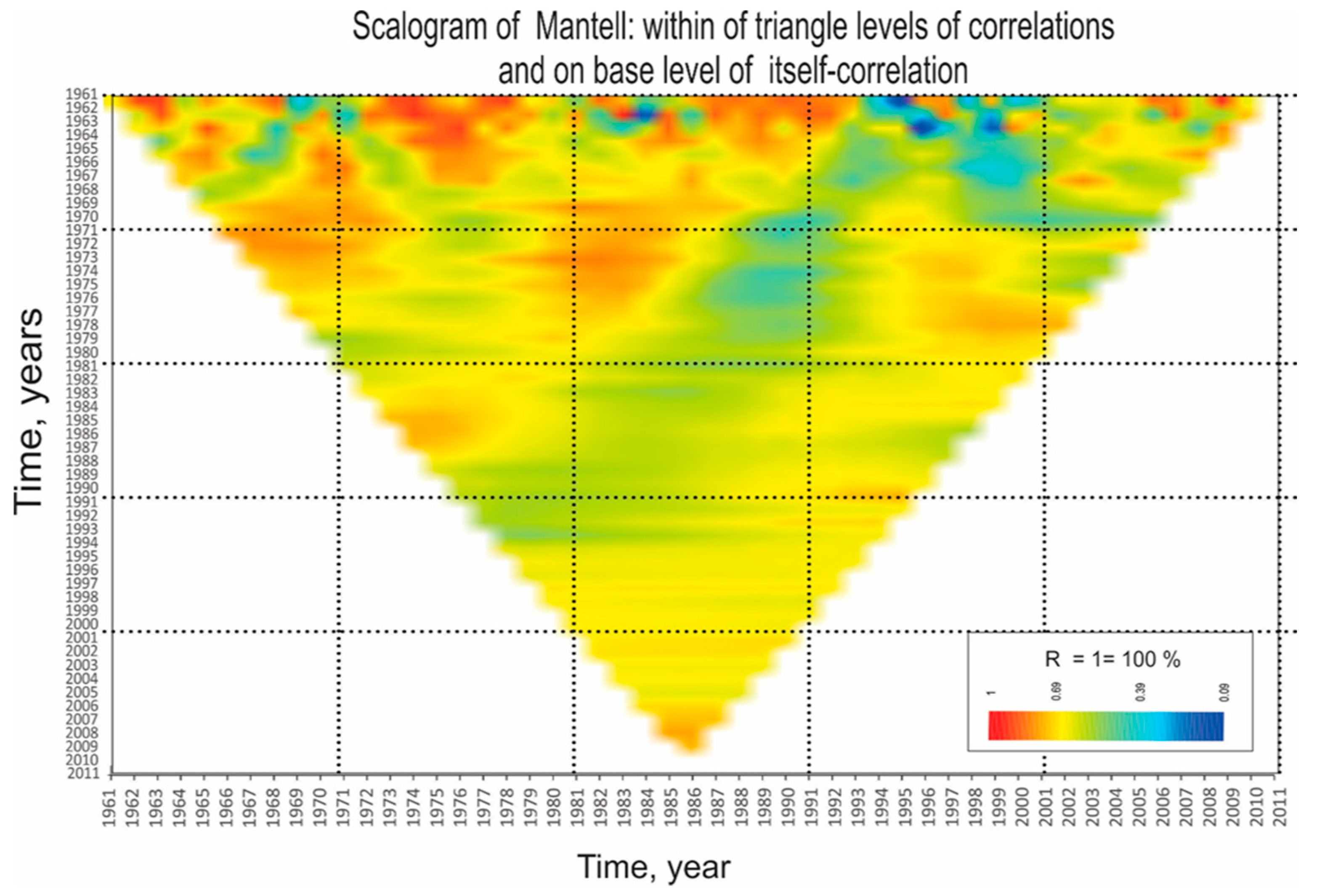
Table 5.
Values obtained from t_stat-DW ranged from 1.85 to 2.15, and the t_stat-DFA for to assess seasonality in the 16 historical datasets. If I(1) was present, it indicated non-seasonality, while its absence indicated seasonality.
Table 5.
Values obtained from t_stat-DW ranged from 1.85 to 2.15, and the t_stat-DFA for to assess seasonality in the 16 historical datasets. If I(1) was present, it indicated non-seasonality, while its absence indicated seasonality.
| Test on Null Hypothesis: variable has a unit root | ||||
| Exogenous: Constant, Linear Trend | ||||
| Lag Length: 0 (Automatic - based on SIC, maxlag = 10) | ||||
| Sample: 1961 2011 Included observations: 51 | ||||
| 5% test critical value = -3.5 | ||||
| Number | Variable | t_Stat_DW * | t_Stat_DFA ** | P(valor) *** |
| 1 | Ahome | 2.020 | -6.250 | 0.001 |
| 2 | Bocatoma | 1.990 | -7.000 | 0.001 |
| 3 | Choix | 1.950 | -6.060 | 0.001 |
| 4 | El Carrizo | 1.970 | -6.270 | 0.005 |
| 5 | El Fuerte | 2.000 | 5.820 | 0.001 |
| 6 | Higuera Zaragoza | 1.960 | -7.005 | 0.004 |
| 7 | Huites | 1.960 | -7.070 | 0.001 |
| 8 | Las Estacas | 2.120 | -5.020 | 0.001 |
| 9 | Los Mochis | 1.980 | -5.930 | 0.001 |
| 10 | Mochicahui | 2.030 | -4.400 | 0.001 |
| 11 | Ocoroni | 1.860 | -6.020 | 0.001 |
| 12 | Presa Josefa Ortiz | 2.120 | -4.940 | 0.001 |
| 13 | Presa Miguel Hidalgo | 1.970 | -6.990 | 0.001 |
| 14 | Ruiz Cortines | 1.950 | -5.510 | 0.000 |
| 15 | Topolobampo | 2.010 | -6.840 | 0.000 |
| 16 | Yecorato | 1.920 | -6.290 | 0.002 |
| * t_stat_DW = Durvin Watson Test Statistical, ** t_stat_DFA = Augmented Dickey Fuller Test Statistical, *** P(value) = Probability Value (respect to α = 0.05) | ||||
Disclaimer/Publisher’s Note: The statements, opinions and data contained in all publications are solely those of the individual author(s) and contributor(s) and not of MDPI and/or the editor(s). MDPI and/or the editor(s) disclaim responsibility for any injury to people or property resulting from any ideas, methods, instructions or products referred to in the content. |
© 2024 by the authors. Licensee MDPI, Basel, Switzerland. This article is an open access article distributed under the terms and conditions of the Creative Commons Attribution (CC BY) license (http://creativecommons.org/licenses/by/4.0/).
Copyright: This open access article is published under a Creative Commons CC BY 4.0 license, which permit the free download, distribution, and reuse, provided that the author and preprint are cited in any reuse.


