
Submitted:
29 December 2024
Posted:
30 December 2024
You are already at the latest version
Abstract
Climate change and increased demand for water are causing supply problems in the Mexico City and State of Mexico. The lack of complete and up-to-date meteorological information makes it difficult to understand and analyze climate phenomena such as droughts. Climate Engine (http://ClimateEngine.org) provides decades of climate data to analyze such changes. In this study, CHIRPS and DAYMET were used to calculate SPEI at scales of 1, 3, 6, 9, 12 and 24 months between 1981 and 2023 in the study area. The Mann-Kendall test for precipitation showed no significant change, while maximum and minimum temperatures showed a significant growth trend, which was reflected in the SPEI values. In the last 10 years, droughts have become more frequent and severe in the western part of the State of Mexico and south of Mexico City. When analyzing the last 14 years, the highest moisture values occurred in 2010, 2015 and 2018, while the most severe drought values were recorded in 2017, 2019, 2020, 2021 and 2023.
Keywords:
Climate engine
; drought index
; CHIRPS
; DAYMET
1. Introduction
Droughts are temporary and recurrent phenomena caused by a lack of precipitation that can affect water availability in a hydrological system [1]. The negative consequences could affect a wide range of social, economic and environmental sectors [2].
Their duration could be short (e.g., a few days or weeks), but they can greatly threaten water supply [3,4] and cause significant reductions in crop yields, especially during critical plant growth stages such as germination, pollination, and grain filling [5,6,7].
The recent technological development of remote sensing techniques and instruments for the spatial monitoring of variables related to the hydrological cycle has made it possible to refine their spatial and temporal resolution, which has resulted in their use as sources of information for drought analysis. This has allowed the creation of drought monitoring and assessment systems at different spatial scales (e.g., regional, national, global). Such systems integrate observations derived from different sources of information (e. g., remote sensing, ground-based radars, gauging stations, etc.) with results from climatological, hydrological and land surface models [8]. From this, it is possible to identify affected regions and response protocols are activated once an event has started [9].
This complexity is due to the difficulty of quantifying the severity of a drought, since we usually identify a drought by its effects on different systems (agriculture, water resources, ecology, forest fires, economic losses, etc.), but there is no specific physical variable that allows us to measure the severity of the drought. Therefore, droughts are difficult to identify in time and space, being very complex to determine the moment when a drought begins and ends, as well as to quantify its duration, magnitude and surface extension [9,10].
Generally, droughts can be divided into four types: meteorological drought, agricultural drought, hydrological drought, and socio-economic drought. Drought indices are available for monitoring regional drought conditions. Over the past few decades, many excellent drought indices have been developed and widely used for drought monitoring. [11]
Drought indices are vital for objectively quantifying and comparing the severity, duration and extent of a drought in regions with varying climatic and hydrological regimes. The Standardized Precipitation Index (SPI), described by McKee [12] and Guttman [13], measures normalized anomalies in precipitation and has been recommended as a key indicator of drought by the World Meteorological Organization [14] and as a universal meteorological index of drought by the Lincoln Declaration on Drought [15].
Most drought indices currently in use are suitable for the detection and assessment of dry and wet conditions on time scales of months or years, while drought indices with shorter time scales (e.g., daily), which are more suitable for drought monitoring and forecasting, are relatively scarce. With the rapidly increasing concurrence of abnormally high temperatures and droughts due to global warming [16,17], sudden droughts occur frequently [18,19].
In Mexico, droughts are monitored with the SPI index [20]. Despite this widespread acceptance, SPI does not consider atmospheric conditions other than precipitation that may affect drought severity, such as temperature, wind speed, and humidity. To address this problem, Vicente-Serrano [21] developed the Standardized Precipitation-Evapotranspiration Index (SPEI). The SPEI uses a similar form, but instead normalizes anomalies in the cumulative climatic water balance, defined as the difference between precipitation and potential evapotranspiration. This modification retains the computational simplicity, multi-temporal nature, and statistical interpretability of SPEI, while providing a more comprehensive measure of water availability that includes a broader measure of climatic conditions.
Understanding climate phenomena requires climatological information, such as rainfall measurements from conventional ground-based weather stations, which are the main sources of such climate data. However, historical records of station observations are inadequate in many parts of the world due to the sparse, decreasing or non-existent network of stations. Therefore, satellite-derived rainfall products are increasingly used as a complement or substitute for station observations [22].
New technologies have provided a complete or just partial but sufficient solution to complement the lack of information and extending to areas that due to time and budget issues would not have been possible to analyze [23].
The State of Mexico and Mexico City face a scarcity of water resources due to the increase in water demand (population growth) and its inefficient use (infrastructure in poor condition and without adequate maintenance). This problem is increased by the effects of climate change that causes low rainfall and recurrent drought phenomena in recent years [24].
The objective of this work is to calculate the SPEI indices for the State of Mexico and Mexico City for a period from 1981 to 2023, using the CHIRPS databases to obtain precipitation data and DAYMET to obtain temperature data.
2. Materials and Methods
2.1. Description of the Study Area
The study area covers the State of Mexico and Mexico City, Figure 1. The State of Mexico has an area of 22,351.8 km2, which represents 1.1% of Mexico's surface area; however, it is the most populated State with 16,992,418 inhabitants. Mexico City (CdMx) has an area of 1,494.3 km2 which represents 0.1% of the country's surface; Mexico City has 9,209,944 inhabitants [25]. The study area is located between 2,250 and 2,750 meters above sea level, the predominant climate is dry temperate, with an average annual temperature of 15.9 °C and an average annual rainfall of 686 mm with a climate known as sub-humid temperate [26].
2.2. Climatological Databases
381 meteorological stations from the National Meteorological System (SMN) station network, Figure 1 were analyzed in Mexico City and the State of Mexico for a period from January 1981 to December 2023 (42 years).
The availability of stations still operating is 59% in the study area; for this reason, the geographic coordinates of each meteorological station served as a reference for the recovery of climatic data in Climate Engine (http://ClimateEngine.org). It was decided to consider the CHIRPS database that presents daily, pentad and monthly data. For the maximum and minimum temperature, they were collected from the DAYMET database, whose values provided are daily and monthly. When analyzing the monthly CHIRPS and DAYMET data for station 15170 in Chapingo with the monthly observed data and those obtained from the CHIRPS database, a R2 = 0.8921 was obtained for precipitation, and for DAYMET, a R2 = 0.9974 was obtained for the maximum temperature and a R2 = 0.9824 for the minimum temperature.
2.3. Homogeneity Test
The statistical characteristics of the hydrological series, such as the mean, standard deviation and serial correlation coefficients, are affected when the series shows a trend in the mean or variance, or when negative or positive jumps occur; such anomalies are produced by loss of homogeneity and inconsistency.
In general, the lack of homogeneity of the data is induced by human activities such as deforestation, opening of new cultivation areas, rectification of riverbeds, construction of reservoirs and reforestation. It is also a product of sudden natural processes, such as forest fires, earthquakes, landslides and volcanic eruptions. Statistical tests that measure the homogeneity of a series of data present a null hypothesis and a rule to accept or reject it [27].
2.4. Mann-Kendall Statistical Test
HydroGeoLogic [28] considers that the Mann-Kendall test is the most appropriate method for analyzing trends in climatological series. Also, this method allows detecting and locating the approximate starting point of a given trend.
The Mann-Kendall test is a non-parametric test [29,30], suggested to evaluate the trend in environmental data series [31]. This test basically consists of the comparison between the values that compose the same time series, in sequential order [32].
If the number of positive pairs is P, and the number of negative pairs is N, then S is defined as S = P - N. For n > 10, a Z statistic can be defined that follows the standard normal distribution where Equation (1) represents the Mann-Kendall test statistic:
The result of S indicates the possible existence of trends, if the value of S is significantly different from zero. S being different from zero, the null hypothesis H0 can be rejected, and the alternative hypothesis H1 would be accepted [30].
2.5. Climate Engine
Climate Engine (htpss://app.climateengine.org) allows non-commercial users of any technical level to take advantage of the cloud storage capabilities to collect Earth observation data. Climate Engine offers specialists the opportunity to go back in time and see how our landscapes have changed due to climate changes over the past decades. It is capable of quantitatively analyzing years of data in a matter of seconds. ClimateEngine.org, which was launched thanks to the White House Climate Data Initiative and a Google Faculty Research award, now plays an essential role in Earth science research and decision support for government agencies and is trusted by thousands of users each month [33].
Climate Engine tools put petabytes of cutting-edge data with easy access. And because Climate Engine tools are backed by Google Earth Engine cloud computing, the analysis possibilities are virtually limitless [34].
The National Oceanic and Atmospheric Administration's (NOAA) National Integrated Drought Information System (NIDIS) supports the use of Climate Engine to assess vegetation condition and satellite-based climate maps at regional and field scales to improve drought monitoring and early warning systems. With several types of regional-scale data currently in use, the use of Climate Engine by U.S. Drought Monitor authors, regulatory agencies, and ranchers and farmers adds local-scale information to assess field-scale impacts such as vegetative drought (short-term soil moisture deficits) and hydrologic drought (long-term water deficits and low streamflow) [35].
2.6. CHIRPS Satellite Data
The CHIRPS algorithm combines three main data sources: (a) the Climate Hazards group precipitation climatology (CHPclim), a global precipitation climatology at 0.05° latitude/longitude resolution estimated for each month from station data, averaged satellite observations, elevation, latitude and longitude [36,37]; (b) satellite precipitation estimates based on thermal infrared precipitation (IRP); and (c) in situ rain gauge measurements. CHPclim differs from other precipitation climatology in that it uses long-term satellite mean precipitation fields as a guide to derive climatological surfaces. This improves its performance in mountainous countries [37].
Additional data from some regions, such as East Africa, the Sahel, Central America and Afghanistan, are also used [23,38]. The procedure for combining CHIRP with station observations uses the expected correlation between the precipitation of a given pixel and that of nearby stations. These correlations are estimated from the CHIRP fields. An additional correlation value is also used, which is assumed to be an estimate of the correlation between the “true” precipitation at each pixel and the CHIRP values [39].
The fusion of station data with CHIRP data is performed on pentad (5-day) and monthly time scales, subsequently re-scaling the pentads to daily level. The preliminary CHIRPS is available 2 days after the end of a pentad, while the final version is generated the third week of the following month.
2.7. DAYMET Satellite Data
Daily Surface Weather Data provides long-term, continuous, gridded estimates of daily weather and climate variables by interpolating and extrapolating ground observations using statistical modeling techniques. Daymet meteorological variables include daily minimum and maximum temperature, precipitation, vapor pressure, shortwave radiation, snow water equivalent, and day length produced over a 1 km x 1 km gridded area over continental North America and Hawaii since 1980 and over Puerto Rico from 1950 to the end of the most recent full calendar year [40].
The Daymet method for estimating daily surface meteorological parameters at locations lacking instrumentation is based on a combination of interpolation and extrapolation, using data from multiple instrumented locations and weights for each location that reflect the spatial and temporal relationships of the estimation location to instrumental observations. The approximate number of instrumental observations to be used for each estimate is defined as a parameter for each of the Daymet primary variables.
As part of a series of algorithm modifications intended to improve robustness in regions of very low station density, the Daymet V4 algorithm abandons the iterative calculation of station density and instead defines a search radius for each estimation location that is sized exactly to capture the average number of input stations, based on precomputed matrices of inter-station distances. Given the preprocessed input station observations and precomputed station lists and interpolation weights for each estimation grid location, two separate workflows are used to produce the primary Daymet output variables: one for the daily temperature variables and one for the daily precipitation variable [40].
2.8. Potential Evapotranspiration Equations
Care was taken to select the most used potential evapotranspiration methods that span the range of equation types, including temperature-based, radiation-based, and combined equations [41]. In order of complexity, these models are Thornthwaite [42], Hargreaves [43], Penman-Montieth with the Hargreaves radiation term referenced here as P-M (Hargreaves) [44], Priestley-Taylor [45] and FAO-56 Penman-Montieth referenced here as P-M (FAO-56) [44]. The FAO-56 reference crop definition [44] is used for all PET models except for the Thornthwaite equation, which uses the original definition of Thornthwaite [42]. The term “PET” is used in all models to maintain consistency with the proposed SPEI definition [21].
Of these methods, the Thornthwaite method is unique because it is based on an empirical relationship between mean monthly temperature and potential evapotranspiration. Despite its differences and limitations [46,47], the Thornthwaite method was included because it is commonly used and was cited in the original SPEI methodology [21]. The rest of the PET methods follow the general form, Equation (2):
where Rn represents the net radiation, γ is the psychrometric constant and Δ is the slope of the vapor saturation-pressure vs temperature curve at the given air temperature. The Hargreaves equation uses the daily difference between Tmax and Tmin as a proxy for estimating net radiation [43] and simplifies the mass transfer term with a constant. The P-M equation (Hargreaves) uses an identical estimate of radiation but evaluates mass transfer using wind speed from the Watch Forcing Dataset [48]. Priestley-Taylor and P-M (FAO56) use net radiation directly from the WFD, although Priestley Taylor simplifies the mass transfer with a constant and the full Penman-Monteith model (P-M FAO56) uses wind speed and atmospheric conditions from the WFD to calculate this term.
2.9. The Palmer Drought Severity Index (PDSI)
The PDSI was a milestone in the development of drought indices. It measures both wetness (positive value) and dryness (negative values), based on the supply and demand concept of the water balance equation, thus incorporating previous precipitation, moisture supply, runoff, and evaporative demand at the surface level. Many of the problems of the PDSI were solved with the development of the self-calibrating PDSI (sc-PDSI) [49], which is spatially comparable and reports extreme wet and dry events with predicted frequencies for infrequent conditions. However, the main shortcoming of PDSI has not been resolved. This is its fixed time scale (between 9 and 12 months), and an autoregressive feature whereby index values are affected by conditions up to four years in the past [13].
2.10. Standardized Precipitation Index (SPI)
The Standardized Precipitation Index (SPI) was proposed by McKee [12]. This index consists of the conversion of precipitation data to probabilities based on long-term precipitation records. The probabilities are transformed into normalized series with an average of 0 and a standard deviation of 1. The main advantage of the SPI over the Palmer indices is that it allows the analysis of drought impacts at different time scales [50], in addition to the identification of different types of droughts, since different natural systems and economic sectors may respond to drought conditions at very different time scales [21,51,52,53]. McKee [12] used the Gamma distribution to transform precipitation series to standardized units. However, Pearson's type III distribution shows a better adaptability to precipitation series computed at different time scales [54,55,56].
The SPI only uses precipitation input without considering temperature and evaporation, and the accuracy of the precipitation dataset affects the SPI accuracy. The SPEI is calculated using the water balance equation, which is the difference between precipitation and potential evapotranspiration. It not only considers the sensitivity of temperature and evaporation to drought, but also retains the characteristics of multiple time scales and comparability [11].
The SPI is calculated by fitting a probability density function to a given frequency distribution of precipitation totals for a station or grid point and for an accumulation period and then the probabilities are transformed into a normalized distribution with a mean equal to zero and a variance of one. SPI is calculated as follows in Equation (3):
where, xi refers to the current precipitation in the examined period, xj refers to the mean precipitation of the timeseries, and σ refers to the standard deviation of the timeseries [57].
SPI can be calculated based on long-term rainfall data for each meteorological station with gamma distribution using the maximum likelihood estimation method for different time scales, i.e., 1, 3, 6, 9, 12, 24, and 48 months [58].
2.11. The Importance of Including Temperature Data
Precipitation-based drought indices, including SPI, are based on two assumptions: i) the variability of precipitation is much greater than that of other variables, such as temperature and potential evapotranspiration (PET), and ii) the other variables are stationary (i.e., they have no temporal trend). In this scenario, the importance of these other variables is negligible, and droughts are controlled by the temporal variability of precipitation. However, some authors have cautioned against systematically neglecting the importance of the effect of temperature on drought conditions. Empirical studies have shown that increasing temperature markedly affects the severity of droughts [59].
The role of warming-induced drought stress is evident in recent studies that have analyzed drought impacts on net primary production and tree mortality [60,61,62,63]. The strong role of temperature in drought severity was evident in the devastating 2003 heatwave in central Europe, where extremely high temperatures dramatically increased evapotranspiration and exacerbated summer drought stress [64], drastically reducing Aboveground Net Primary Production (ANPP) [65]. Similar patterns were observed in the summer of 2010 with a strong heat wave that increased drought stress in forests and produced large forest fires in Eastern Europe and Russia [66]. Thus, empirical studies have shown that rising temperatures increase drought stress and increase forest mortality in situations of low rainfall [67]. Warming processes are also probably the triggering factor for the decline in global agricultural production observed in recent years [68]. Thus, to illustrate how warming processes are reinforcing drought stress and related ecological impacts worldwide, Breshears [69] coined the term global change-type drought to refer to drought under global warming conditions.
Over the past 150 years there has been a general increase in temperature (0.5 – 2 °C), and climate change models predict a marked increase during the 21st century. This is expected to have dramatic consequences for drought conditions, with an increase in water demand due to evapotranspiration.
Therefore, it is preferable to use drought indices that include temperature data in their formulation (such as the PDSI), especially for applications involving future climate scenarios. However, the PDSI lacks the multi-scale character essential both for assessing drought in relation to different hydrological systems and for differentiating between different types of droughts. Therefore, a new drought index (the Normalized Precipitation Evapotranspiration Index; SPEI) has been formulated based on precipitation and PET. The SPEI combines the sensitivity of the PDSI to changes in evaporative demand (caused by temperature fluctuations and trends) with the computational simplicity and multi-temporal nature of the SPI.
The SPEI cannot identify the role of temperature increase in future drought conditions, and regardless of global warming scenarios it cannot account for the influence of temperature variability and the role of heat waves. SPEI can account for potential effects of temperature variability and extreme temperatures beyond the context of global warming. Therefore, given the lower additional data requirements of SPEI relative to SPI, it is preferable to use the former for drought identification, analysis and monitoring in any climatic region of the world [70].
2.12. Standardized Precipitation Evapotranspiration Index (SPEI)
The SPEI meets the requirements of a drought index, as its multi-scale nature allows it to be used by different scientific disciplines to detect, monitor and analyze droughts.
The standardized precipitation evapotranspiration index (SPEI) is similar to SPI except for the addition of the mean minimum and mean maximum temperature to rainfall. In the SPEI calculation, we need the monthly water balance, which is based on the difference between rainfall and potential evapotranspiration (PET). [58]
Like the sc-PDSI and the SPI, the SPEI can measure drought severity based on its intensity and duration and can identify the beginning and end of drought episodes. The SPEI allows for comparison of drought severity over time and space, as it can be calculated in a wide range of climates, just like the SPI. Furthermore, Keyantash and Dracup [71] indicated that drought indices should be statistically robust and easy to calculate and have a clear and understandable calculation procedure. All these requirements are met by the SPEI. However, a crucial advantage of the SPEI over other widely used drought indices that consider the effect of PET on drought severity is that its multi-scale features allow for the identification of different drought types and impacts in the context of global warming.
A reduction in precipitation due to climate change will affect the severity of droughts. Both the sc-PDSI and the SPI identify the influence of a reduction in precipitation on future drought conditions. Because of the decrease in precipitation, recorded droughts increase in maximum intensity, total magnitude and duration. In contrast, wet periods will show the opposite behavior. Therefore, both indices could record changes in droughts related to changes in precipitation.
However, climate change scenarios also show an increase in temperature during the 20th century. In some cases, such as the A2 greenhouse gas emissions scenario, the models predict an increase in temperature that could exceed 4 °C with respect to the 1960-1990 average.
The differences between the sc-PDSI using real data and the two modelled series are also shown. This simple experiment clearly shows an increase in the duration and magnitude of droughts at the end of the century, which is directly related to the increase in temperature. No similar pattern could be identified using the SPI, demonstrating the shortcomings of this widely used index in addressing the consequences of climate change [59].
The use of drought indices that include temperature data in their formulation (e.g. the Palmer Drought Severity Index PDSI) to identify drought impacts on different ecological, hydrological and agricultural systems, although it lacks the multi-scale character essential for the assessment of drought in different systems, and for differentiating between types of droughts. The SPEI [21], based on precipitation and potential evapotranspiration records, combines the sensitivity of the PDSI to changes in evaporative demand, with the simplicity of calculation and the multi-temporal nature of the Standardized Precipitation Index (SPI).
The Standardized Precipitation and Evapotranspiration Index (SPEI) is an extension of the widely used SPI. The SPEI is designed to account for both precipitation and potential evapotranspiration (PET) to quantify drought and thus capture the main impact of rising temperatures on water demand.
The procedure for calculating the SPEI is similar to the one used for the SPI. However, the SPEI uses the difference between precipitation and reference evapotranspiration (P – ETo), rather than precipitation (P) as input. The climatic water balance compares available water (P) to atmospheric evaporative demand (ETo) and therefore provides a more reliable measure of drought severity than considering precipitation alone. ETo is the evapotranspiration rate from a reference surface (e.g. a hypothetical well-watered reference crop of grass with specific characteristics).
The SPEI uses a climatic water balance (Di = Pi – ETo) calculated for several time scales (k) (i.e. for one month, two months, three months, etc.). For example, to obtain the 6-month SPEI, a time series is first constructed by summing the D values from five months ago to the current month.
The original formulation of the SPEI suggested the use of the Thornthwaite equation for the estimation of ETo [42]. This equation only requires the mean daily temperature and the latitude of the site and was used due to limited data availability. However, other alternative equations can be used. The more robust FAO-56 Penman-Monteith equation [44] is recommended if data (relative humidity, temperature, wind speed and solar radiation) are available. If the data required for this equation is not available, the Hargreaves equation (first option) or the Thornthwaite equation (second option) are recommended. Differences between the SPEI series calculated using the different equations to estimate ETo can be significant in some regions of the world. In general, these differences were greater in semi-arid areas and smaller in humid regions [72]. In this work, the SPEI calculation was performed in the RStudio® program [73] using the SPEI.R package version 1.8.1, developed by Beguería and Vicente [72], at time scales of 1, 3, 6, 9, 12 and 24 months, with data on precipitation, minimum and maximum temperature, latitude of the study point analyzed, and the Hargreaves method was selected for the calculation of evapotranspiration.
The values obtained were analyzed based on the SPEI classification and categories [12] Table 1. With this information, a temporal analysis was carried out, with the aim of understanding the evolution of droughts; identifying periods of moderate, severe and extreme drought; and defining their intensity, duration, and approximate start and end dates.
3. Results
The test was performed at the 381 points used as reference from the 381 meteorological stations that served as location for the recovery of the climatic data collected for precipitation, maximum and minimum temperature using the Mann-Kendall test. The homogeneity test found that most of the monthly precipitation data were homogeneous with 71.13% with a non-significant increasing trend and 28.87% with a non-significant decreasing trend of the total precipitation values. For the maximum temperature, it was found that 87.93% were values with a significant increasing trend, 10.50% with a non-significant increasing trend and 1.57% with a non-significant decreasing trend. The monthly minimum temperature had a 67.98% significant increasing trend, 27.56% non-significant increasing trend and 4.46% non-significant decreasing trend. The tests performed detect whether the series or record is homogeneous, because it has no persistence or trend, change in the mean, or does not fluctuate too much. The results of these tests are presented with TSC for a significant increasing trend, TNSC for a non-significant increasing trend, TNSD for a non-significant decreasing trend, and TSD for a significant decreasing trend. The variables analyzed were precipitation, maximum temperature, and minimum temperature. A significant change in the mean is evidence of some impact by an external phenomenon, whether natural or man-made Figure 2.
Taking this into account, the drought analyzed was continued by calculating SPEI of the area with the meteorological records previously analyzed statistically. In general, the analysis of the SPEI values was carried out for the different time scales of 1, 3, 6, 9, 12 and 24 months in a period of 42 years, from 1981 to 2023 for the maximum and minimum values.
An analysis was carried out on the 3-month SPEI drought index from 2010 to 2023, which refers to the average accumulated precipitation in a 3-month period and is compared with the historical average precipitation in that same period. Positive SPEI values indicate a surplus of water content, that is, the land is receiving more water than it loses through evaporation. Negative values indicate a precipitation deficit, that is, the land is receiving less water than it loses through evaporation, Figure 3.
The 3-month SPEI drought index is a useful indicator to assess the severity of droughts in different regions and time scales, considering evaporation and accumulated precipitation over a 3-month period.
Figure 4 shows the severity of 6-month droughts for the years 2019 to 2023, with the drought being most severe in the western part of the State of Mexico, where the capital of the State of Mexico, Toluca, and the Cutzamala system that supplies drinking water to Mexico City are located (Figure 5). A three-month drought index should trigger a drought management program, but a six-month drought index is a cause for greater concern because a longer drought begins to affect aquifer recharge. Figure 5 shows the comparison of the SPEI-6-month indices, 1981-2023, for two stations located in the West and East of the State of Mexico; note that since 2015, droughts, measured through negative value indices, are more severe in the western part of the State of Mexico, where the capital Toluca and the Cutzamala system that supplies water to Mexico City are located. The word climate change is still a bit controversial, and sometimes it is preferred to call it “climate trends”; the results of drought can be natural trends and/or the influence of anthropogenic activity. The truth is that analyzing the INEGI reports on land use for the years 2009 and 2018 for the state of Mexico, the areas with human settlements, including large cities, have increased by 62% [30]. Likewise, the bare soil surface has tripled, and the agricultural area has decreased by 0.6% (61,500 ha). From 2009 to 2018, 2,600 hectares of forests have been lost. Surely in other parts of Mexico, changes in land use continue, and although they occur in other states, ultimately we live in an ecosystem, where what you do in one place finds echo in other parts, for example the famous phenomenon of El Niño and La Niña originate in the Oceans, such as in South America and end up having an echo in the distribution of temperature and rainfall in Mexico.
4. Discussion
There is sufficient evidence that the temperature in the study area over the 42-year period had a significant increase in most of the areas, the effect of which was reflected in the calculated SPEI values at the different time scales. The global warming level approach has its limitations when variables that respond quickly to warming, such as temperature and precipitation, are taken into consideration since they show little dependence on the scenario [74].
These extreme drought values began in 2010, when the maximum humidity levels did not occur in years with excess humidity compared to other years analyzed. The effects on the lack of moisture recovery are linked to changes in the area, such as the increase in urban areas and the reduction of crops and forest areas. This lack of homogeneity in the data was induced by human activities such as deforestation and not by any sudden natural process, such as forest fires, earthquakes, landslides and volcanic eruptions.
Taking this into account, the recovery of aquifers in the area is threatened by the increasing demand for water resources while the supply is affected by the conditions of the area and the climate. Authorities must take these observations into account because the areas most affected by the drought are those considered to be the areas of aquifer recharge and the most important supply system for Mexico City, which is the Cutzamala system.
5. Conclusions
The homogeneity tests provided evidence that, in the period of analysis, there is an upward trend in the values of minimum and maximum temperature. The lack of homogeneity is caused by human activities and may also be the product of a sudden natural process that, in this case, in the study area, human intervention has caused an increase in maximum and minimum temperatures in the 42 years analyzed.
This increase in temperature was reflected in the SPEI value for the region analyzed, because it captures the main impact of the increase in temperatures on water demand. Because of the increase in temperatures, the recorded droughts increase in maximum intensity, total magnitude and duration. On the contrary, the wet periods will show the opposite behavior.
Between the period of 1981 - 1985, 1988 - 1991 and 1998 - 2014 there were droughts considered as moderately dry, but the one in 1998 was the longest, which had short periods of three years of recovery in 2004 and 2008 with values considered close to normal, most of which were categorized as moderately dry and very dry.
In the last 14 years for a 3-month analysis, it was possible to see that the years with the highest humidity values were 2010, 2015 and 2018, with the year 2021 and 2023 having a moderate recovery of humidity, however, the years with the most severe drought were 2017, 2019, 2020, 2021 and 2023 as a consequence of the increase in temperatures and a constant in precipitation.
This indicates that the severity of the drought in recent years has been more severe and its recovery less severe, as a greater amount of area has been categorized as extremely dry and very dry.
Institutional Review Board Statement
Not applicable
Informed Consent Statement
Not applicable
Data Availability Statement
The data presented in this study are available on request from the corresponding author. The data are not publicly available due to privacy.
Acknowledgments
To the National Council of Humanities, Science and Technology, CONAHCYT, of Mexico for the financial support provided in the form of a postgraduate maintenance scholarship for the development of this research.
Conflict of Interest
The authors declare no conflicts of interest.
References
- Smakhtin, V. U. & Schipper, E. L. F. 2008 Droughts: the impact of semantics and perceptions. Water Policy 10 (2), 131.
- Stahl, K., Kohn, I., Blauhut, V., Urquijo, J., de Stefano, L., Acácio, V., Dias, S., Stagge, J. H., Tallaksen, L. M., Kampragou, E., van Loon, A. F., Barker, L. J., Melsen, L. A., Bifulco, C., Musolino, D., de Carli, A., Massarutto, A., Assimacopoulos, D. & van Lanen, H. A. J. 2016 Impacts of European drought events: insights from an international database of text-based reports. Natural Hazards and Earth System Sciences 16 (3), 801–819.
- Dai A. 2011b. Drought under global warming: A review. WIREs Clim Change, 2: 45–65.
- Zhang Q, Yao Y B, Li Y H, Huang J P, Ma Z G, Wang Z L, Wang S P, Wang Y, Zhang Y. 2020. Progress and prospect on the study of causes Zhang X, et al. Sci China Earth Sci February (2022) Vol.65 No.2 335 and variation regularity of droughts in China. Acta Meteorol Sin, 78: 500–521.
- Meyer S J, Hubbard K G, Wilhite D A. 1993. A crop-specific drought index for corn: I. Model development and validation. Agron J, 85: 388–395.
- Calviño P A, Andrade F H, Sadras V O. 2003. Maize yield as affected by water availability, soil depth, and crop management. Agron J, 95: 275–281.
- Hunt E D, Svoboda M, Wardlow B, Hubbard K, Hayes M, Arkebauer T. 2014. Monitoring the effects of rapid onset of drought on non-irrigated maize with agronomic data and climate-based drought indices. Agric For Meteorol, 191: 1–11.
- Real-Rangel R. A., Pedrozo-Acuña A., Breña-Naranjo J. A., Alcocer-Yamanaka V. H. 2017. Monitorización de sequías en México a través del índice estandarizado multivariado de sequía. XXIV Congreso Nacional de Hidráulica. Acapulco, Guerrero, México, marzo 2017.
- Wilhite, D.A., (2000): Drought as a natural hazard: concepts and definitions. In Drought: a global assessment. (D. Wilhite ed.). Vol 1: 3-18.
- Burton, I., R.W. Kates, and G.F. White, (1978): The environment as hazard. Oxford University Press. Nueva York, 240 pp.
- Sun, Y.; Chen, X.; Yu, Y.; Qian, J.; Wang, M.; Huang, S.; Xing, X.; Song, S.; Sun, X. Spatiotemporal Characteristics of Drought in Central Asia from 1981 to 2020. Atmosphere 2022, 13, 1496. [CrossRef]
- McKee, T. B., Doesken, N. J. & Kleist, J. (1993) The relationship of drought frequency and duration to time scales. In: Proceedings of the 8th Conference on Applied Climatology. American Meteorological Society Boston, MA, pp. 179–183.
- Guttman, N.B., (1998): Comparing the Palmer drought index and the Standardized Precipitation Index. Journal of the American Water Resources Association, 34, 113-121.
- WMO (2006) Drought monitoring and early warning: Concepts, progress and future challenges. WMO.
- Hayes, M., Svoboda, M., Wall, N. & Widhalm, M. (2011) The Lincoln declaration on drought indices: universal meteorological drought index recommended. Bulletin of the American Meteorological Society 92(4), 485–488.
- Hao Z, AghaKouchak A, Phillips T J. 2013. Changes in concurrent monthly precipitation and temperature extremes. Environ Res Lett, 8: 034014.
- Ren L, Zhou T, Zhang W. 2020. Attribution of the record-breaking heat event over Northeast Asia in summer 2018: The role of circulation. Environ Res Lett, 15: 054018.
- Wang L Y, Yuan X. 2018. Two types of flash drought and their connections with seasonal drought. Adv Atmos Sci, 35: 1478–1490.
- Yuan X, Wang Y M, Zhang M, Wang L Y. 2020. A few thoughts on the study of flash drought (in Chinese). Trans Atmos Sci, 43: 1086–1095.
- Monitor de Sequía en México. Servicio Meteorológico Nacional. 2024. https://smn.conagua.gob.mx/es/climatologia/monitor-de-sequia/monitor-de-sequia-en-mexico. Date of consultation: october 30, 2024.
- Vicente-Serrano, S. M., Beguería, S. & López-Moreno, J. I. (2010) A multi-scalar drought index sensitive to global warming: the standardized precipitation evapotranspiration index – SPEI. J. Climate 23, 1696–1718.
- Dinku T, Funk C, Peterson P, et al. Validation of the CHIRPS satellite rainfall estimates over eastern Africa. Q J R Meteorol. Soc. 2018; 144 (Suppl. 1):292–312. [CrossRef]
- Funk, C., Peterson, P., Landsfeld, M., Pedreros, D., Verdin, J., Shukla, S., Husak, G., Rowland, J., Harrison, L., Hoell, A. and Michaelsen, J. 2015a. The climate hazards group infrared precipitation with stations - A new environmental record for monitoring extremes. Scientific Data, 2, 150066. [CrossRef]
- CONAGUA (Comisión Nacional del Agua). 2014. Programa de medidas preventivas y de mitigación de la sequía. Consejo de Cuenca ríos Fuerte y Sinaloa (pp. 262). Ciudad de México, México: Comisión Nacional del Agua, Secretaría de Medio Ambiente y Recursos Naturales.
- INEGI monografías. 2024. https://cuentame.inegi.org.mx/monografias/ . Date of consultation november 4, 2024.
- INEGI (Instituto Nacional de Estadística, Geografía e Informática). 2023. 2020 Censo de Población y Vivienda. México. https://www.inegi.org.mx/datosabiertos/.
- Escalante-Sandoval, Carlos A., Reyes-Chávez, Lilia. 2002. Cap.7 Análisis de frecuencias de eventos extremos, Técnicas estadísticas en hidrología. UNAM: Facultad de Ingeniería, México, pp: 129-130. ISBN 970-32-0173-3.
- HydroGeoLogic, Inc.-OU-1 Informe anual de monitoreo de aguas subterráneas de 2004: antiguo Fort Ord, California, 2005.
- Kendall, M. G. 1975. Rank correlation methods. Charles Griffin. London. p.120.
- Mann, H. B. 1945. Nonparametric tests against trend. Econometrica 13, 245-259.
- Yu, J.-Y., & Kao, H.-Y. 2007. Decadal changes of El Niño persistence barrier in SST and ocean heat content indices: 1958-2001. Geophysical Research Letters.
- Silva, D. G. 2007. Evolução Paleoambiental dos Depósitos de Tanques em Fazenda Nova, Município de Brejo da Madre de Deus - Pernambuco. (Dissertação de Mestrado). Recife: UFPE.
- Climate Engine. 2024. Desert Research Institute and University of California, Merced. Recover april 2024. http://climateengine.org, version 2.1.
- Huntington, J., Hegewisch, K., Daudert, B., Morton, C., Abatzoglou, J., McEvoy, D., and T., Erickson. 2017. Climate Engine: Cloud Computing of Climate and Remote Sensing Data for Advanced Natural Resource Monitoring and Process Understanding. Bulletin of the American Meteorological Society, http://journals.ametsoc.org/. [CrossRef]
- Google Earth and Earth Engine. 2019. Climate Engine maps and time series help scientists and managers see and study earth observation data. Recover abril 2024. https://medium.com/google-earth/climate-engine-maps-and-time-series-help-scientists-and-managers-see-and-study-earth-observation-d59496444475.
- Funk, C., Michaelsen, J. and Marshall, M. 2012. Mapping recent decadal climate variations in precipitation and temperature across Eastern Africa and the Sahel. In: Wardlow, B., Anderson, M. and Verdin, J. (Eds.) Remote Sensing of Drought—Innovative Monitoring Approaches. London: Taylor and Francis, pp. 331–357.
- Funk, C., Verdin, J., Michaelsen, J., Peterson, P., Pedreros, D. and Husak, G. 2015b. A global satellite assisted precipitation climatology. Earth System Science Data Discussions, 7, 1–13. [CrossRef]
- Funk, C., Peterson, P., Landsfeld, M., Pedreros, D., Verdin, J., Rowland, J., Romero, B., Husak, G., Michaelsen, J. and Verdin, A. 2014. A quasi-global precipitation time series for drought monitoring. U.S. Geological Survey Data Series, 832, 4. [CrossRef]
- Maidment, R., Grimes, D., Black, E. et al. A new, long-term daily satellite-based rainfall dataset for operational monitoring in Africa. Sci Data 4, 170063 2017. [CrossRef]
- Thornton, M.M., R. Shrestha, Y. Wei, P.E. Thornton, S-C. Kao, and B.E. Wilson. 2022. Daymet: Daily Surface Weather Data on a 1-km Grid for North America, Version 4 R1. ORNL DAAC, Oak Ridge, Tennessee, USA. [CrossRef]
- McMahon, T. A., Peel, M. C., Lowe, L., Srikanthan, R. & McVicar, T. R. (2013). Estimating actual, potential, reference crop and pan evaporation using standard meteorological data: a pragmatic synthesis. Hydrol. Earth Syst. Sci. 17, 1331–1363.
- Thornthwaite, C. W. (1948). An approach toward a rational classification of climate. Geographical review 38(1), 55–94.
- Hargreaves, G. H. & Samani, Z. A. (1985) Reference crop evapotranspiration from ambient air temperature. American Society of Agricultural Engineers, 96–99.
- Allen, R., Pereira, L., Raes, D. & Smith, M. (1998) Crop evapotranspiration. FAO irrigation and drainage paper 56. FAO, Rome, Italy, 10.
- Priestley, C. H. B. & Taylor, R .J. (1972) On the assessment of surface heat flux and evaporation using large-scale parameters. Mon. Weather Rev. 100(2), 81–92.
- Jensen, M. E. (1973) Consumptive Use of Water and Irrigation Water Requirements. New York.
- Amatya, D., Skaggs, R. & Gregory, J. (1995) Comparison of methods for estimating REF-ET. J. Irrig. Drain. Div. ASCE, 121(6): 427-435.
- WFD. Hadley Centre for Climate Prediction and Research/Met Office/Ministry of Defence/United Kingdom. 2018. WATer and global CHange (WATCH) Forcing Data (WFD) - 20th Century. Research Data Archive at the National Center for Atmospheric Research, Computational and Information Systems Laboratory. Revised abril 2024. [CrossRef]
- Wells, N., S. Goddard, and M.J. Hayes, 2004: A self-calibrating Palmer Drought Severity Index. Journal of Climate 17, 2335-2351.
- Edwards, D.C. and McKee, T.B., (1997): Characteristics of 20th century drought in the United States at multiple time scales. Atmospheric Science Paper No. 634.
- Vicente-Serrano, S.M. and López-Moreno, J.I., (2005), Hydrological response to different time scales of climatological drought: an evaluation of the standardized precipitation index in a mountainous Mediterranean basin. Hydrology and Earth System Sciences 9: 523-533.
- Vicente-Serrano, S.M. (2007), Evaluating The Impact Of Drought Using Remote Sensing In A Mediterranean, Semi-Arid Region, Natural Hazards, 40: 173-208.
- Pasho, E., J. Julio Camarero, Martín de Luis and Vicente-Serrano, S.M. (2011) Impacts of drought at different time scales on forest growth across a wide climatic gradient in north-eastern Spain. Agricultural and Forest Meteorology. 151: 1800-1811.
- Guttman, N. B. (1999) Accepting the Standardized Precipitation Index: A Calculation Algorithm. J. Am. Water Resour. Assoc. 35(2), 311–322.
- Vicente-Serrano, S.M., (2006), Differences in spatial patterns of drought on different time scales: an analysis of the Iberian Peninsula. Water Resources Management 20: 37-60.
- Quiring, S.M. (2009): Developing objective operational definitions for monitoring drought. Journal of Applied Meteorology and Climatology 48: 1217-1229.
- Politi, N.; Vlachogiannis, D.; Sfetsos, A.; Nastos, P.T.; Dalezios, N.R. High Resolution Future Projections of Drought Characteristics in Greece Based on SPI and SPEI Indices. Atmosphere 2022, 13, 1468. [CrossRef]
- Moazzam, M.F.U.; Rahman, G.; Munawar, S.; Farid, N.; Lee, B.G. Spatiotemporal Rainfall Variability and Drought Assessment during Past Five Decades in South Korea Using SPI and SPEI. Atmosphere 2022, 13, 292. [CrossRef]
- Schneider, D. P., C. Deser, J. Fasullo, and K. E. Trenberth, 2013: Climate Data Guide Spurs Discovery and Understanding. Eos Trans. AGU, 94, 121–122, https://. [CrossRef]
- Williams AP, Xu Ch, McDowell NG (2011) Who is the new sheriff in town regulating boreal forest growth?. Environmental Research letters 6: . [CrossRef]
- Martínez-Villalta J, López BC, Adell N, Badiella L, Ninyerola M (2008) Twentieth century increase of Scots pine radial growth in NE Spain shows strong climate interactions. Global Change Biology 14: 2868–2881.
- McGuire AD, et al. (2010) Vulnerability of white spruvce tree growth in interior Alaska in response to climate variability: ddendrochronological, demographic, and experimental perspectives. Canadian Journal of Forest Research, 40: 1197-1209.
- Linares JC, Camarero JJ (2011) From pattern to process: linking intrinsic water-use efficiency to drought-induced forest decline. Global Change Biology 18: 1000-1015.
- Rebetez M, et al. (2006) Heat and drought 2003 in Europe: A climate synthesis. Annals of Forest Science 63: 569-577.
- Ciais Ph, et al. (2005) Europe-wide reduction in primary productivity caused by the heat and drought in 2003. Nature 437: 529-533.
- Barriopedro D, Fischer EM, Luterbacher J, Trigo RM, García-Herrera R (2011) The hot summer of 2010: Redrawing the temperature record map of Europe. Science 332: 220-224.
- Adams HD, et al. (2009) Temperature sensitivity of drought-induced tree mortality portends increased regional die-off under global-change-type drought. Proceedings of the National Academy of Sciences of the United States of America 106: 7063-7066 (2009).
- Lobell DB, Schlenker W, Costa-Roberts J (2011) Climate trends and global crop production since 1980. Science 29: 616-620.
- Breshears DD, et al. (2005) Regional vegetation die-off in response to global-change-type drought. Proceedings of the National Academy of Sciences of the United States of America 102: 15144-15148.
- Vicente-Serrano, Sergio M. & National Center for Atmospheric Research Staff (Eds). 2024 "The Climate Data Guide: Standardized Precipitation Evapotranspiration Index (SPEI).” Recover abril, 2023 de https://climatedataguide.ucar.edu/climate-data/standardized-precipitation-evapotranspiration-index-spei.
- Keyantash, J. and J. Dracup., 2002: The quantification of drought: an evaluation of drought indices. Bulletin of the American Meteorological Society 83, 1167-1180.
- Beguería, S., & Vicente, S. 2014. Calculation of the Standardized Precipitation-Evapotranspiration Index. Package SPEI.R for R or RStudio Program. https://cran.r-project.org/web/packages/SPEI/index.html. (Recover: may 2023).
- RStudio, Inc. 2023. RStudio® Version 2023.03.1 Boston: RStudio, Inc.
- Alba, V.; Russi, A.; Caputo, A.R.; Gentilesco, G. Climate Change and Viticulture in Italy: Historical Trends and Future Scenarios. Atmosphere 2024, 15, 885. [CrossRef]
Figure 1.
Location of the State of Mexico, Mexico City, and the 381 weather stations operated by the SMN.
Figure 1.
Location of the State of Mexico, Mexico City, and the 381 weather stations operated by the SMN.
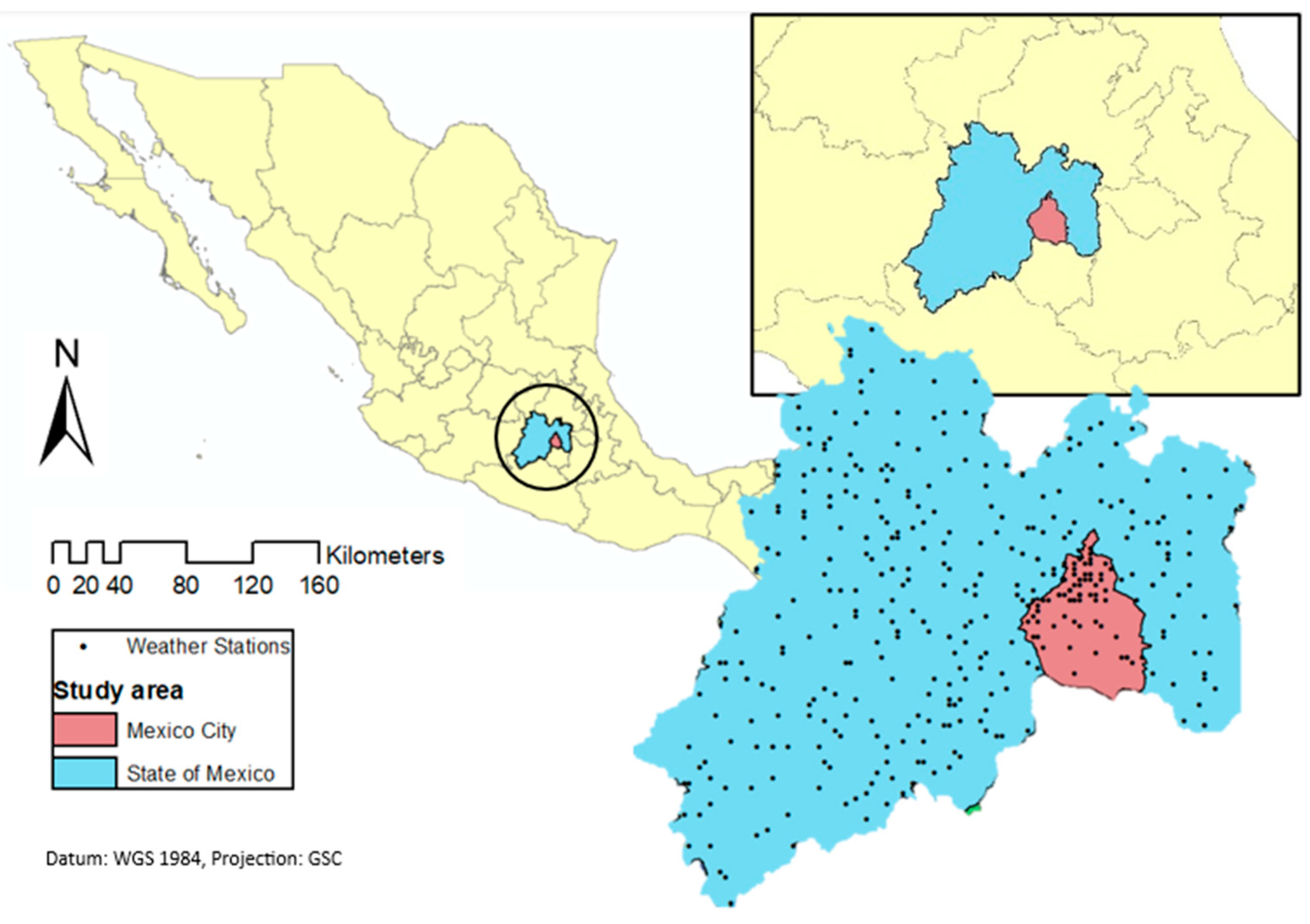
Figure 2.
Trends in the variables analyzed in the study area (TSC = significant increasing trend; TSD = significant decreasing trend; TNSC = non-significant increasing trend).
Figure 2.
Trends in the variables analyzed in the study area (TSC = significant increasing trend; TSD = significant decreasing trend; TNSC = non-significant increasing trend).
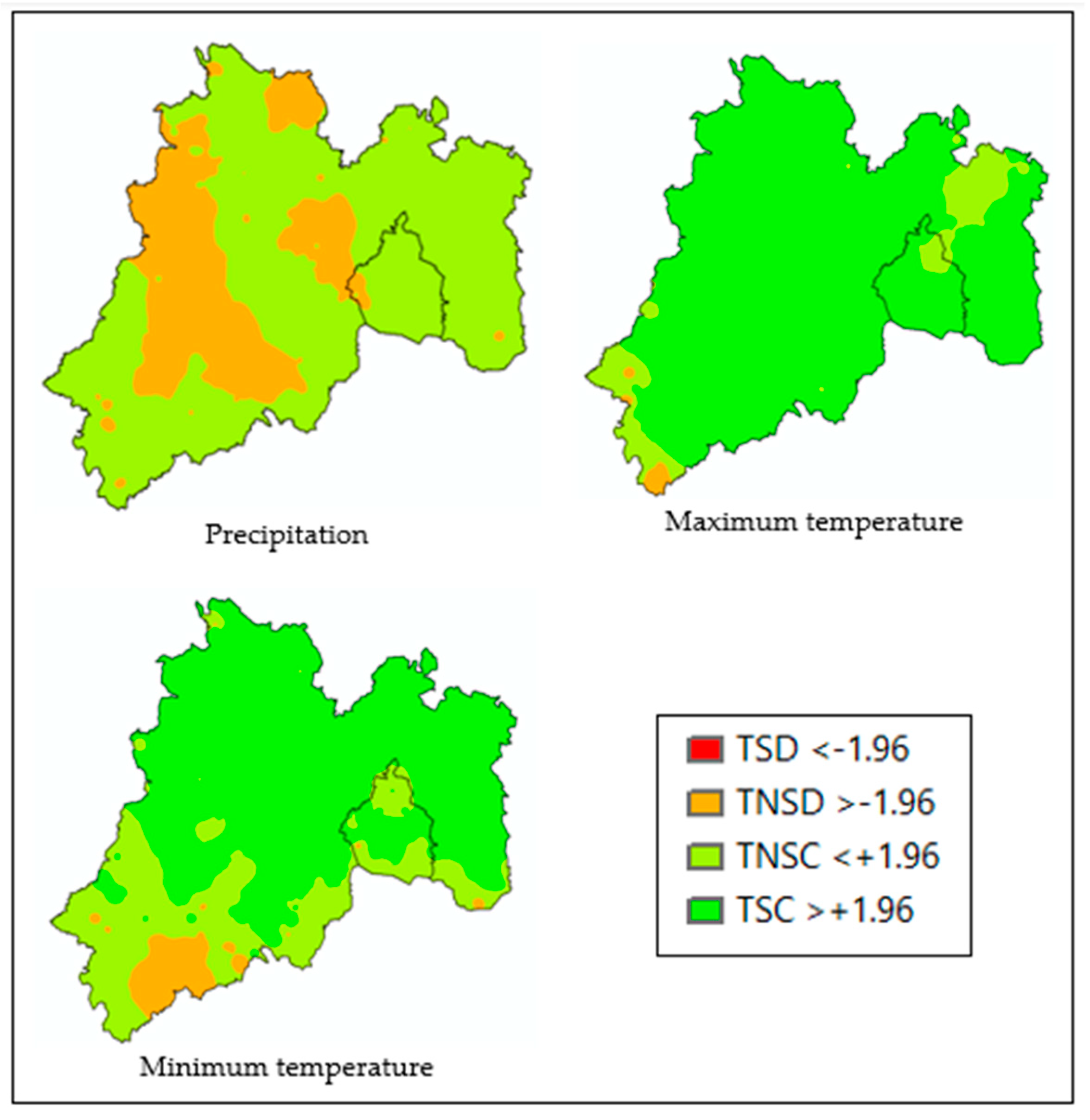
Figure 3.
Spatial distribution of maximum and minimum SPEI values calculated for a 3-month time scale (2010-2023).
Figure 3.
Spatial distribution of maximum and minimum SPEI values calculated for a 3-month time scale (2010-2023).
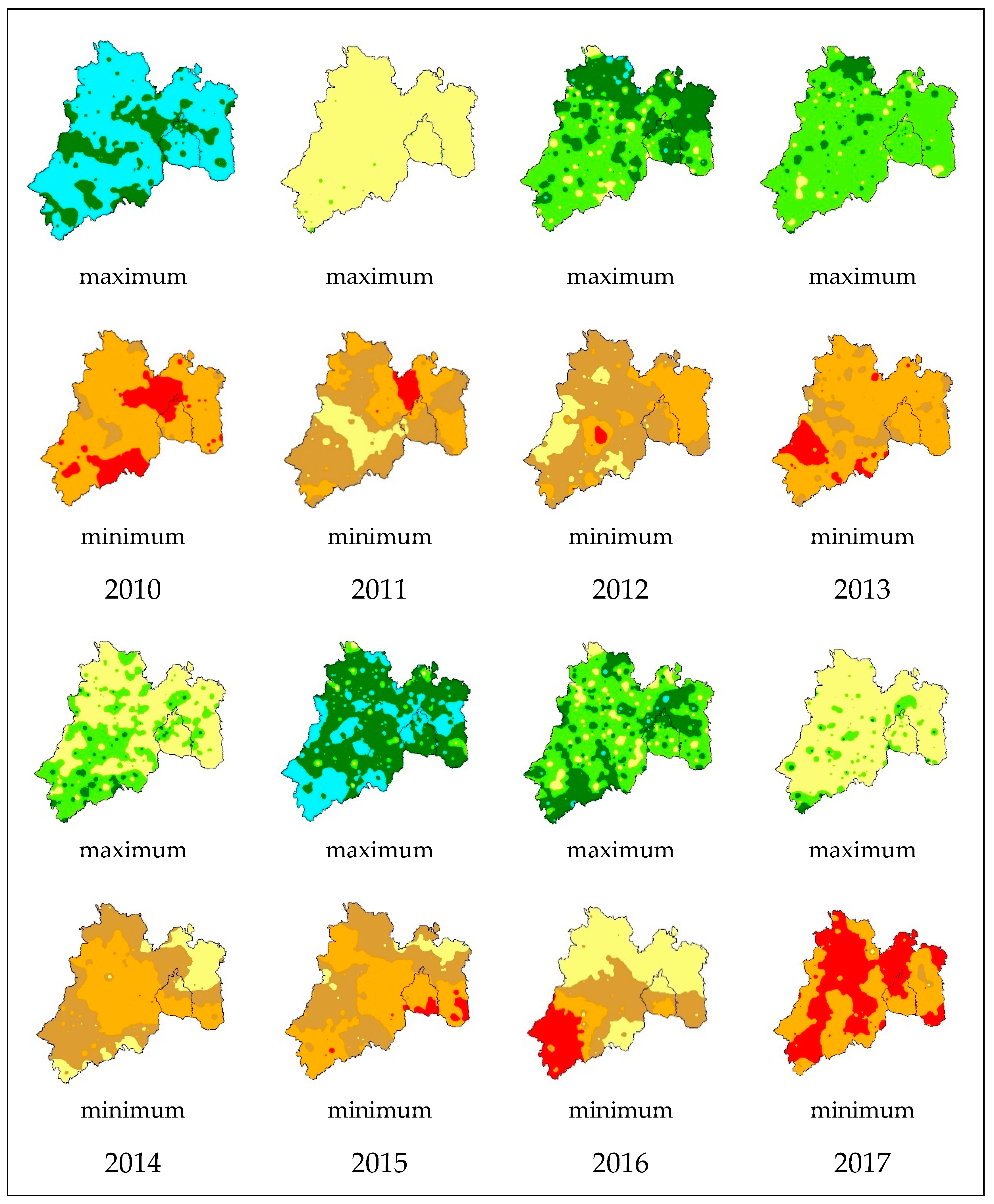
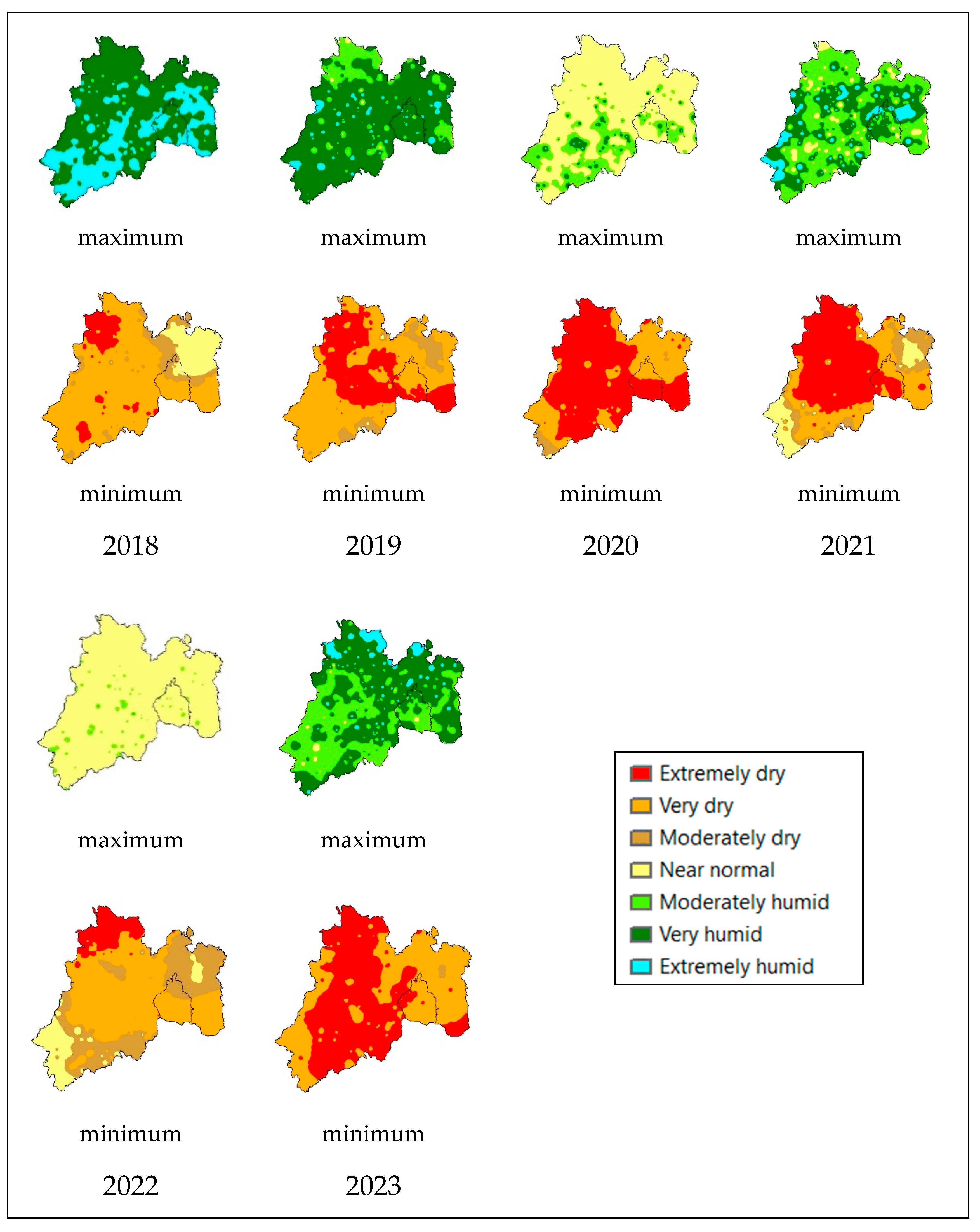
Figure 4.
The most severe six-month drought indices in Mexico City and the State of Mexico from 2016 to 2023.
Figure 4.
The most severe six-month drought indices in Mexico City and the State of Mexico from 2016 to 2023.
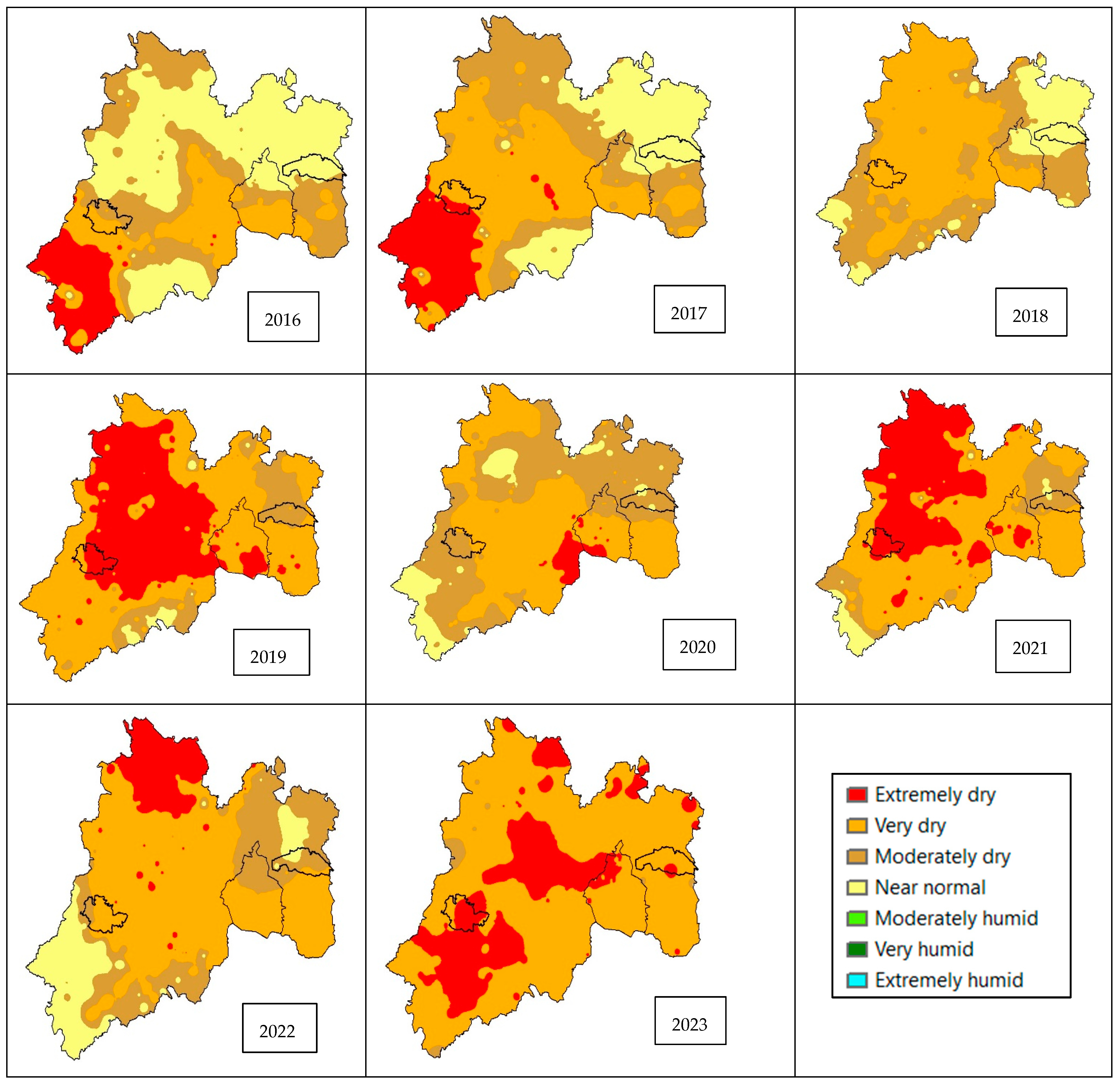
Figure 5.
Temporal variation of the 6-month SPEI index comparing a station in the West (Valle de Bravo) with a station in the East (Texcoco) of the State of Mexico.
Figure 5.
Temporal variation of the 6-month SPEI index comparing a station in the West (Valle de Bravo) with a station in the East (Texcoco) of the State of Mexico.
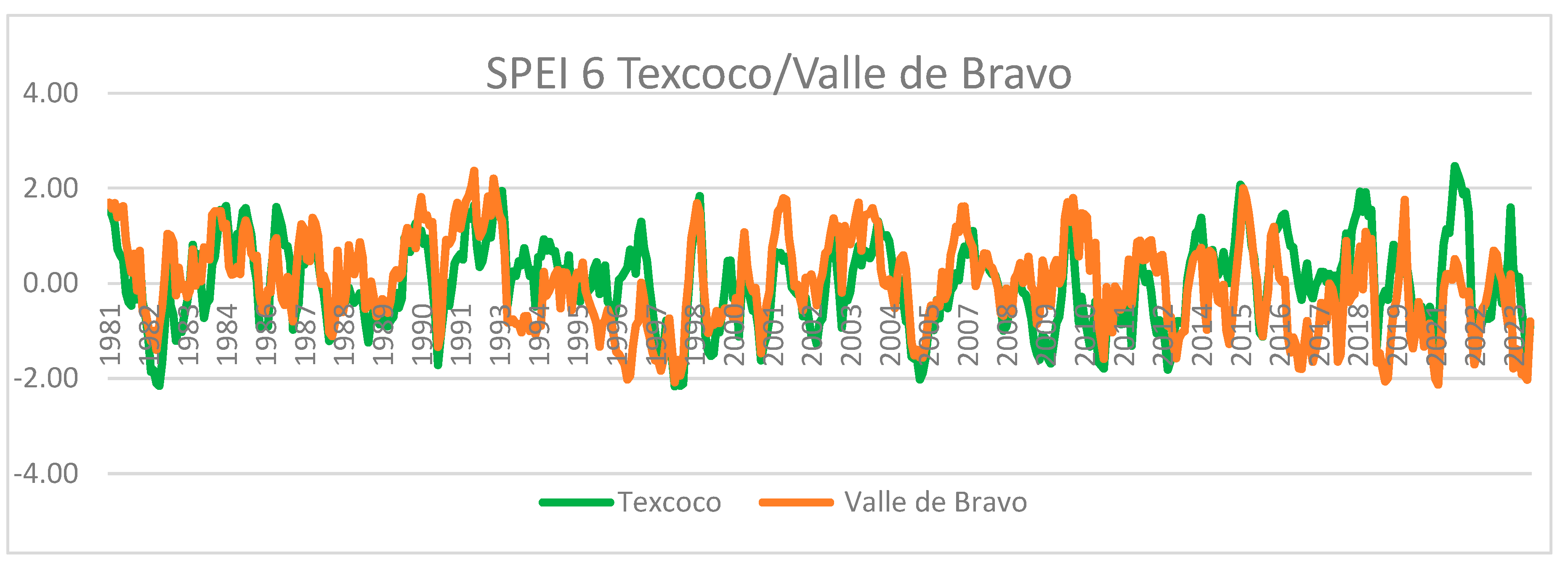

Table 1.
SPEI categories and classification [12].
Table 1.
SPEI categories and classification [12].
| Index value | Category |
| > 2.00 | Extremely humid |
| 1.50 to 1.99 | Very humid |
| 1.00 to 1.49 | Moderately humid |
| -0.99 to 0.99 | Near normal |
| -1.00 to -1.49 | Moderately dry |
| -1.50 to -1.99 | Very dry |
| < -2.00 | Extremely dry |
Disclaimer/Publisher’s Note: The statements, opinions and data contained in all publications are solely those of the individual author(s) and contributor(s) and not of MDPI and/or the editor(s). MDPI and/or the editor(s) disclaim responsibility for any injury to people or property resulting from any ideas, methods, instructions or products referred to in the content. |
© 2024 by the authors. Licensee MDPI, Basel, Switzerland. This article is an open access article distributed under the terms and conditions of the Creative Commons Attribution (CC BY) license (http://creativecommons.org/licenses/by/4.0/).
Copyright: This open access article is published under a Creative Commons CC BY 4.0 license, which permit the free download, distribution, and reuse, provided that the author and preprint are cited in any reuse.


