

Submitted:
01 March 2024
Posted:
05 March 2024
You are already at the latest version
Abstract
This paper presents a quantum formulation for classical abstract dynamical systems (ADS), defined by coupled sets of first order differential equations. They are referred as “abstract” because their dynamical variables can be of different interrelated nature, not necessarily corresponding to physics, such as populations, socioeconomic variables, behavioural variables, etc. A first order classical Hamiltonian in canonical moments can be derived for ADS by using Dirac’s dynamics for singular Hamiltonian systems. And also a corresponding first order Schrödinger equation (which involves the existence of a system Planck constant particular of each system) can be derived from this Hamiltonian. However, Bohm and Hiley’s reinterpretation of quantum mechanics produces no further information about the mathematical formulation of ADS. However, a second order classical Hamiltonian in canonical moments can be also derived for ADS, as well as a corresponding second order Schrödinger equation. In this case, Bohm and Hiley’s reinterpretation of quantum mechanics provides a quantum Hamiltonian that does provide the quantum formulation for ADS, which provides new quantum variables interrelated dynamically with the classical variables. An application case is presented: the one-dimensional autonomous system given by the logistic dynamics, where the differences between the classical and the quantum trajectories are highlighted.
Keywords:
dynamical systems
; general systems
; classical dynamics
; Schrödinger equation
; quantum formulation
; Bohm and Hiley’s interpretation
; quantum dynamics
; logistic function.
1. Introduction
General System Theory was proposed by Bertalanffy [1] as a new complementary approach to Science in order to provide it of a mathematical universal language. Since that work, some attempts to state a General System Theory have been provided. For a summary of these attempts see [2]. However, the objective to provide that universal language seems by the moment too ambitious and it has been steered to provide general systems as theories that unify different fields of Science. An example is provided by the work [3] that proposes a unified mathematical view of energy in psychology and physics. The method followed in [3] is the so-called isomorphism of systems proposed by Ferrer [4], i.e., translating a known contrasted theory from a field to another field where similar problems try to be solved.
The present paper objective holds the isomorphism of systems proposal: translating the quantum formalism from dynamics of physical systems to abstract dynamical systems. Note that the dynamical systems in physics are defined generally by Newton laws, i.e., by coupled sets of second order differential equations. However, abstract dynamical systems are here referred as dynamical models given by coupled sets of first order differential equations, where the unknown temporal variables have different interrelated nature, not necessarily corresponding to physics, such as populations, socioeconomic variables, behavioural variables, etc. Actually, these systems are known in the literature about the subject simply as dynamical systems (see for example the work by Anosov and Arnold [5]). However, including the adjective abstract presents the transdisciplinary aspect of this kind of systems. This question must be emphasized because, for instance, a system Planck constant is presented in the formalism, and it is not the physical Planck constant, but a singular constant of the particular system under study.
A first attempt of a (non-relativistic) quantum formalism for abstract dynamical systems was presented by this author’s paper in [6], but he did not reach any significant solution. Then, this paper tries to present a significant solution to that objective from a rigorous mathematical approach, although no empirical support has yet been found. Therefore, this paper tries to open a new field of research, which lies between General System Theory and mathematical-physics, by presenting the theoretical finding obtained.
To reach that formalism the well-known method to obtain the Schrödinger equation from the Hamiltonian is also followed. Then, the first step is to obtain the Hamiltonian for an abstract dynamical system. The method followed is what discovered by Dirac [7], who provides a method to obtain a Hamiltonian for which the canonical moments either cannot be explicitly isolated from the general velocities (i.e., the time derivatives of the configuration variables) or the canonical moments vanish. This last case is also known as a singular system, and it is which corresponds to an abstract dynamical system, as it is showed in this work.
Actually, the real objective of Dirac in the work [7] was to quantize the electromagnetic field due to it is given by first order partial differential equations. Therefore, it was an approach steered to solve the problem for fields rather for abstract dynamical systems. However, getting the Hamiltonian for abstract dynamical systems can also be solved with this Dirac’s formalism. See the works [8,9,10] for that solution, although only in [6,9] the subsequent quantization method is presented in two different ways: from a first order Hamiltonian in the canonical moments in [6], and from a second order Hamiltonian in the canonical moments in [9]. The differences about the Hamiltonian formulated by first or second order in canonical moments are clarified throughout this paper.
Besides Hamiltonian Dirac’s approach, there exists a Lagrangian approach provided by Havas [11], who obtains equivalent results to the Hamiltonian Dirac’s approach of [7]. Govaerts highlighted that equivalence for first order fields in [12] and it was also highlighted for abstract dynamical systems in [8]. Both problems are known in mathematical-physics respectively as the inverse Lagrange problem and as the inverse Hamiltonian problem. In other words, the inverse Lagrange problem consists in finding the Lagrangian corresponding to a coupled set of differential equations; therefore, this set must obey the Euler-Lagrange equations. Besides, inverse Hamiltonian problem consists in finding the Hamiltonian that holds the Hamilton equations; therefore, this set must obey the Hamilton equations.
Havas presents the inverse Lagrange problem solution for abstract dynamical systems in the Annex B of [11] from a set of general sufficient equations that solve the inverse Lagrange problem for a more significant number of differential systems. Those sufficient solutions were presented in a previous work [13], where a wide range of general inverse Lagrange problems were dealt and solved. However, Micó in [8] solves the inverse Lagrange problem for abstract dynamical systems by following a simpler way and also showing the equivalence with the corresponding inverse Hamiltonian problem by Dirac’s method [7].
Besides, the paper’s objective enounced as translating the quantum formalism from dynamics of physical systems to abstract dynamical systems, can be brought further by the Bohm and Hiley’s reinterpretation of quantum mechanics [14]. This reinterpretation provides a quantum potential correction to the classical equations through the quantum Hamilton-Jacobi. In fact, the quantum Hamilton-Jacobi equation arises from the polar form of the quantum wave function and its split in modulus, which provides the probability conservation, and in phase or action, which provides the quantum Hamilton-Jacobi equation. Bohm and Hiley linked this correction to the existence of a microscopic level underlying the quantum level of description. However, the present paper tries to interpret a possible quantum correction of abstract dynamical systems as a quantum term which arises rather from the own system complexity. In addition, a system Planck constant, particular of each system studied and then with different value of physical Planck constant, is presented in the formalism. Then, the formalism presented assumes an epistemological correction to the dynamics of an abstract dynamical system, playing a fundamental role the system Planck constant. Also that incapability is present in Bohm and Hiley’s formalism [14], but as emphasized above, due to the assumption of a microscopic world underlying the quantum level. In this paper this incapability is only assumed in advance as a hypothetical epistemological principle. In fact, throughout the paper, the usual predictions of the abstract dynamical systems are called as classical dynamics, while the predictions of the abstract dynamical systems quantum correction are called as quantum dynamics. Also, depending on the context, classical dynamics can be referred as classical trajectory, and quantum dynamics can be referred as quantum trajectory.
In addition, Dirac’s first order Hamiltonian in canonical moments is showed here that provides, by using the quantization rules, a first order Schrödinger equation that has not a Bohm and Hiley’s quantum potential correction. Therefore, the solution found is applying the same method provided by Dirac in [7] to a second order Hamiltonian in canonical moments. To do this, the abstract dynamical system must be previously reformulated as a second order abstract dynamical system (by taking the time derivative). In addition, some abstract masses are needed to obtain the second order Hamiltonian in canonical moments. In fact, the corresponding Hamilton equations are Newtonian-kind equations where the abstract masses play the same role as the masses in the physical systems. In the subsequent step, a canonical transformation is needed to simplify the Hamiltonian. This further Hamiltonian provides, by using again the quantization rules, a second order Schrödinger equation for which the action does provide the Bohm and Hiley’s quantum potential correction. Finally, the first order abstract dynamical system can be recovered: the quantum potential correction arises as an integral term. This integral term can be represented by a new system of first order differential equations coupled with the original ones.
Besides, one of the most important theory about abstract dynamical systems is referred as synergetics, term coined by Haken [15]. This formalism is probably the closest to here presented. In fact, it provides a partial differential equation, the Fokker-Planck equation, for a stochastic abstract dynamical equation, given by Ito equations (see also [15]), which plays a similar role to Schrödinger equation in Hamiltonian systems. The Fokker-Planck equation provides the time evolution of the probability density. However, the starting point is stochastic, not deterministic, such as the case here presented.
In fact, the deterministic or stochastic character of the formalism presented must be commented. In the present work, the approach is deterministic, i.e., the quantum correction of abstract dynamical systems is applied by deterministic dynamics, although the approach could be also stochastic in future works, due to the quantum potential is derived from the previous wave function, which has a stochastic nature. In fact, both differenced cases are considered in the Bohm and Hiley’s work [14]. This deterministic quantum correction is studied in the application case of Section 7. In this case, the quantum potential presents singularities that highlight the profound differences between the concept of classical trajectory and the quantum trajectory here provided.
In order to present the formalism announced, Section 2 is devoted to the first order Dirac’s Hamiltonian in canonical moments for an abstract dynamical system. In Section 3, the corresponding first order Schrödinger equation is obtained, showing that no quantum potential correction arises in the Hamiltonian. Therefore, Section 4 is devoted to obtain a second order Dirac’s Hamiltonian in canonical moments for an abstract dynamical system. Section 5 makes use of this Hamiltonian to obtain the corresponding second order Schrödinger equation, which does present a quantum potential correction in the Hamiltonian. Section 6 presents the quantum formulation of the abstract dynamical systems from the corresponding quantum Hamilton equations. Section 7 presents an application case: the one-dimensional autonomous system given by the logistic dynamics. Section 8 is devoted to the paper discussion and conclusions.
2. First Order Dirac’s Hamiltonian
An abstract dynamical system is defined by the following coupled set of differential equations ():
In Eq. 1 is the time variable and
represent the dynamical variables. Their nature can be arbitrary, not necessarily of physical nature, such as populations, chemical or biochemical species, socioeconomic or behavioural indicators, etc. In addition, the () represent their dynamical interactions, considering in advance equipped by all kinds of smoothness properties to develop suitably the formalism. In addition, are called as the dynamical velocities.
Following the methodology developed by Dirac [7] for fields, the works [8,10] applied it to obtain a Hamiltonian to abstract dynamical systems. The method presented in those works is also here presented due to they are needed in the subsequent sections. Such as noted Dirac in [7], a Lagrangian for Eq. 1 is only possible if it is linear in the dynamical velocities, that is:
In Eq. 2, the and functions are still undetermined. The corresponding canonical moments are then defined as ():
Note in Eq. 3 the first problem: the canonical moments do not depend on the dynamical velocities, thus the dynamical velocities cannot be isolated from the canonical moments. However, in addition, applying the Hamiltonian definition:
Note in Eq. 4 that the canonical moments are represented as . Besides the first problem provided by Eq. 3, Eq. 4 shows a second problem: the Hamiltonian does not depend on the canonical moments. Due to these two problems is referred as singular. The Dirac method [7] consists in solving both problems by, first, defining the primary constants as ():
And subsequently reinserting the primary constants in the Hamiltonian as the usual way of the (still undetermined) Lagrangre multipliers ():
Note that the Dirac method to reinsert the canonical moments implies that, in the context of the Hamiltonian , the primary constants are not identically zero, but when they are applied in the Hamilton equations. Therefore, the Hamilton equations become ():
Note that, comparing Eqs. 1 and 7, the simplest solution is: (). Then, the Hamilton Eqs. 7 and 8 become ():
In order to determine the and functions, the so-called by Dirac as consistency conditions, (), are applied. Then, from Eq. 5:
The substitution of Eqs. 9 and 10 in Eq. 11 provides, taking into account the zero value of the primary constraints, and after some calculations ():
In Eq. 12 the following functions can be defined ():
Therefore, Eq. 12 can be rewritten by using Eq. 13 as ():
In order to obtain an equation for the functions without the function, such as in Eq. 14, the following steps are followed: 1. Take the partial derivative respect an arbitrary in Eq. 14; 2. Rewrite Eq. 14 by replacing l by j; 3. Take the partial derivative respect in the rewritten equation; 4. Subtract both equations. Taking into account the equality of both crossed derivatives, the result is ():
Therefore, the process to obtain the and functions of the Hamiltonian given by Eq. 8 is: 1. Get the functions by Eq. 15; 2. Substitute these results in Eq. 13 to get the functions; 3. Substitute these results in Eq. 14 to get the function. Take into account in this process that
and that (i.e, it is antisymmetric functional matrix).
However, two different classes of solutions must be considered depending on the system dimension n. This is due to the antisymmetric definition of the functions. On the one hand, if n is even, then, in general . In this case Eqs. 14 or 15 are independent. On the other hand, if n is odd, then always , and being for the n-1 even dimension, one of the Eq. 14 is dependent on the others, which makes that some functions become undetermined parameters from which the rest ones depend on.
Actually, this last case always happens due to Eq. 14 is a coupled set of n equations and n+1 unknown variables: () and . For instance, let the special one-dimensional (n=1) odd case be. The consistence conditions that provide Eq. 14 become:
Note that Eq. 16 does not provide the
multiplying function. When this case happens, the Dirac’s method
[7] prescription is to consider the equations such as Eq. 16 as secondary constraints. In order to get the multiplying function in an equation, the time derivative is taken in Eq. 16:
Taking into account the Hamilton equations of Eqs. 9 and 10, as for the primary constraints, Eq. 17 becomes, after some calculations:
Note in Eq. 18 that just an equation is provided for two unknown variables, and , then one of the two variables become undetermined, and therefore, different solutions can be applied.
Now, with all the formalism developed, the
() and functions can be found, and the Hamiltonian can be written from Eqs. 7 and 8, as:
Observe in addition that, if the action is represented by , the corresponding Hamilton-Jacobi equation for this Hamiltonian is:
Note that in Eq. 20: .
On the other hand, Eqs. 13-15 are deduced by Havas in Annex 2 of [11] for the Lagrangian of Eq. 2, which provides that both approaches, Lagrangian and Hamiltonian, are equivalent, such as Govaerts demonstrates in [12] for fields. Also Micó in [8] deduces both formalisms and demonstrates their equivalence for the abstract dynamical systems here dealt. However, the odd n case is solved by Havas [11] and Micó [8] by adding the differential equation . With this new equation, n+1 is even and, in general, , becoming independent Eqs. 14 and 15, such as it happens in the even n case.
3. First Order Schrödinger Equation
Again, in order to provide a self-contained work, the results of [6] to obtain the quantum approach to the abstract dynamical systems given by Eq. 1, are here also provided. If is the quantum operator corresponding to a known Hamiltonian , the Schrödinger equation is written as:
In Eq. 21 is the wave function. Due to the Hamiltonian is that corresponding to an abstract dynamical system such as Eq. 19,
represents the system Planck constant different of the current Planck constant of physics. Then, the hypothesis assumed is that each abstract dynamical system has its own system Planck constant, whose value represents a limitation of the mathematical knowledge on the system. In addition, following the quantization rules provided for the Copenhagen formalism of the quantum theory [16], is an operator that acts on the wave function as:
Such that in Eq. 22: , , and . Note in Eq. 22 that the term provides that the Hamiltonian is a self-adjoint operator [16].
Then, the first order Schrödinger equation corresponding to the Hamiltonian of Eq. 19 is written as:
Note that Eq. 23 is a first order partial differential equation, contrary to the physical problems where it is second order. However, following Bohm and Hiley’s approach [14]: does Eq. 23 provide a new information for Eq. 1 through a quantum potential arising in Hamiltonian? To answer this question, splitting the wave function in its amplitude and its phase is needed:
The substitution of Eq. 24 in Eq. 23 provides, respectively for the real and the imaginary parts of the equation (after some easy operations and cancelling the term ):
Dividing Eq. 25 by and dividing Eq. 26 by and subsequently multiplying it by :
Eq. 27 provides the Hamilton-Jacobi equation of Eq. 20, corresponding to the Hamiltonian of Eq. 19, for the phase , and Eq. 28 provides the probability conservation for the square amplitude , being the vector of components () the probability current density. Note that contrary to the physical systems, despite that the probability conservation holds, a quantum potential in the Hamiltonian of Eq. 19 does not arise in this context, which would produce a further quantum term (following Bohm and Hiley’s approach) in the original abstract dynamical system of Eq. 1. Thus, the Schrödinger equation Eq. 23 does not provide further mathematical information to Eq. 1.
Therefore, is there any possibility to obtain a second order Schrödinger equation for the abstract dynamical systems of Eq. 1? The answer is positive, but previously a reformulation of Eq. 1 as a second order differential equation system is necessary, as well as finding the corresponding Hamiltonian that will be second order in canonical moments (referred as second order Hamiltonian). This is the objective of the following section.
4. Second Order Dirac’s Hamiltonian
As “second order”, this section is referred as second order in canonical moments, unlike to Eq. 19, which is first order in abstract canonical moments. Then, a corresponding second order formulation is needed instead the original Eq. 1. This alternative second order is presented as a Newtonian-kind equation by multiplying previously Eq. 1 by a set of functions (), here called as abstract masses (still unknown), and subsequently taking the time derivative, that is ():
The Dirac method [7] is also applied here to get the second order Hamiltonian in canonical moments corresponding to Eq. 29. To do this, the starting Lagrangian is also that of Eq. 2, and also the corresponding Hamiltonian of Eq. 6 with the primary constants (). However, due to the multipliers () can also depend on the canonical moments (the Dirac’s method permits it), then, the further hypothesis now assumed is that they have the following form ():
Inserting Eq. 30 in the Hamiltonian of Eq. 6:
Note in Eq. 31 that also, in addition of the functions, the and functions are still undetermined, i.e., they are not here obtained by Eqs. 13-15, due to the new hypothesis of Eq. 30. Taking into account that outside the Hamiltonian expression the primary constants are , the corresponding Hamilton equations for Eq. 31 are ():
Observe that multiplying Eq. 32 by , taking the time derivative, and substituting Eq. 33:
Comparing Eq. 34 with Eq. 29, multiplied by 2, and substituting from Eq. 32, the following equations arise ():
Applying the consistency conditions, (), and taking into account the zero values of the primary constants outside the Hamiltonian expression in the Hamilton equations Eq. 32 and 33 ():
From the last term of Eq. 36 equal to zero, the following terms can be isolated ():
And the left hand terms () of Eq. 35 can be substituted by the right hand terms () of Eq. 37:
Note from Eq. 38 that the following results hold ():
In addition, Eq. 37 can be rewritten as:
Then, from Eq. 40, the following sufficient conditions are assumed to be held:
And from Eq. 39 in Eqs. 41 and 42:
Note that both sets of Eqs. 43 and 44 must be obeyed in order that the Hamiltonian of Eq. 31 holds for Eqs. 29, which are an equivalent second order formulation of Eq. 1.
Note in addition that, by Eq. 43, these abstract masses can be arbitrary as long as they obey it. In addition, they also could be chosen by a question of practical or theoretical convenience. For instance, if the field derived from a potential, then the abstract masses could be all taken equal to unit or constant values. Also the can be arbitrary as long as it obeys Eq. 44. Also in addition, it could be chosen by a question of practical or theoretical convenience. For instance, if the dynamical system was autonomous, i.e., , then the abstract masses could be all taken as
and . However, a general solution for the abstracts masses can be provided: , being constants with the suitable dimensions. Then, Eq. 43 holds identically and it can be also considered that
.
Substituting Eq. 39 in Eq. 31, the second order Hamiltonian arises:
And the corresponding Hamilton equations given by Eq. 32 plus the substitution of Eq. 39 in Eq. 33 ():
Note that Eqs. 43 and 44 must be obeyed in Eqs. 45-47. However, to obtain the second order corresponding Schrödinger equation by applying the quantization rules [16] on the Hamiltonian of Eq. 45, imaginary terms such those of Eq. 23’s second right hand arise, due to the terms proportional to () in Eq. 45. These terms make that the corresponding time-independent second order Schrödinger equation be non-real. Then, a canonical transformation is needed on Eqs. 45-47 to cancel these terms. The proposed canonical transformation is ():
To prove that Eq. 48 is a canonical transformation the following matrix equation must be obeyed [17]:
In Eq. 49, ( is the transposed matrix of ), and are the following dimensional matrices:
In Eq. 50 is the identity matrix and is the null matrix. Taking into account Eq. 48, the
matrix and its transposed matrix become:
Where in Eq. 51 , , and , . Then, the left hand side of Eq. 49 becomes:
However, in Eq. 52, , ; but all these terms are zero due to Eq. 43. Therefore, Eq. 49 holds, and the proposed transformation in Eq. 48 is canonical, i.e., it preserves the Hamilton equations.
In order to get the transformed Hamiltonian, , from the previous Hamiltonian, , the generating function, , is needed. The three functions are related by the following equations [17]:
Taking into account Eq. 48, , then, from Eq. 53: , i.e., . Besides, from Eq. 48 in Eq. 54: , thus, , i.e., , and also, from Eq. 48: . In addition, from Eq. 48 in Eq. 55:
; thus, taking as the independent variables, the primary constants in Hamiltonian of Eq. 44 become, by Eq. 48, (), and the transformed Hamiltonian, also taking into account Eq. 48, becomes:
Note in Eq. 56 that the term must be computed. To do this, note that from the above result that: . However, from Eqs. 44 and 48: ; then, comparing both results: . Therefore, the transformed Hamiltonian becomes:
Observe that in this transformed Hamiltonian, the function obeys Eq. 44 due to the change in the dynamical variables is the identity, i.e., (). For the same reason, the same assertion can be done about the relationships of Eq. 43 that the abstract masses must obey.
From now on, for the sake of simplicity, the expressions of the dynamical velocities and of the canonical moments are recovered for the, i.e., → , → , and also for the expression of the Hamiltonian,
→ . Therefore, Eq. 46 is rewritten as:
Here, the fact that Eqs. 43 and 44 must be held in this last Hamiltonian is emphasized. However, if the abstract dynamical system of Eq. 1 is autonomous, the abstract masses can be chosen, by Eq. 43, as time-independent, and by Eq. 44, as it has been pointed out above. Then, the Hamiltonian of Eq. 58 becomes a time-conserved magnitude, which, as in the physical context, is called here as energy and represented by . Its expression form Eq. 57 is therefore:
Also, the Hamilton-Jacobi equation corresponding to the Hamiltonian of Eq. 58 is:
In addition, taking into account that the transformed primary constraints are zero outside the Hamiltonian of Eq. 58, i.e., (), the corresponding Hamilton equations of this Hamiltonian are ():
To end this section, the proof that the second order version (Eq. 29) of original Eq. 1 is recovered from Eqs. 61 and 62, is provided. Isolating from Eq. 61 and taking the time derivative, it can be equalled to Eq. 62, by also using Eq. 44, that is ():
And after handling Eq. 63, taking into account Eq. 61 ():
Note in Eq. 64 that the first and second terms of the right hand equation are the same by expanding the total time derivative of the first term, therefore:
Dropping the term 2 in Eq. 65, Eq. 29 is recovered. This deduction is important to be compared with the deduction made in the following section. There, the quantum potential (obtained from the second order Schrödinger equation) changes significantly Eq. 29, and also the original Eq. 1.
5. Second Order Schrödinger Equation
As “second order”, this section is referred to the second order partial derivatives respect the dynamical variables of the Schrödinger equation. They arise by applying the quantization rules [16] to the canonical moments of the Hamiltonian of Eq. 58, once the primary constants are substituted (that is, the second equality of Eq. 58), taking into account that in Eq. 58 the canonical moments are now second order. Therefore, if is the quantum operator corresponding to the Hamiltonian of Eq. 58 (its second equality), the Schrödinger equation is written again as:
In Eq. 66 is the wave function, where σ represents again the system Planck constant, with the same sense commented in Section 2. In addition, following the quantization rules provided by the Copenhagen formalism of the quantum theory [16], is an operator that acts on the wave function as:
Such that in Eq. 67: , and . Note that the term provides that the Hamiltonian is a self-adjoint operator (see [18] for this case, which is not dealt in [16]). In fact, by making explicit this operator in Eq. 67, and subsequently in Eq. 66, the second order Schrödinger equation arises:
If the abstract dynamical system of Eq. 1 is autonomous, the abstract masses can be chosen, by Eq. 43, as time-independent, and by Eq. 44, as it has been pointed out in Section 4. Therefore, the time-independent second order Schrödinger equation corresponding to Eq. 68 can be found by the current substitution , where corresponds to the system energy of Eq. 59, that is:
In order to find out if some quantum potential arises from the second order Schrödinger equation (Eq. 68), then, as in Eq. 24, the wave function split in its amplitude and its phase is done:
Such as it has been done in Section 3, the substitution of Eq. 70 in Eq. 68 provides an equation for the real part and another equation for the imaginary part (after some operations and cancelling the term ):
Dividing the first one by and dividing the second one by and subsequently multiplying it by :
In Eq. 73, is the quantum potential, whose expression is:
Therefore, Eq. 73 represents the quantum Hamilton-Jacobi equation
[14], due to the difference with the Hamilton-Jacobi equation of Eq. 60 is the quantum potential of Eq. 75. In addition, Eq. 74 represents the conservation of the probability density provided by , being the vector of coordinates () the current density.
6. The Quantum Hamilton Equations and the Quantum Formulation of the Abstract Dynamical Systems
By comparing the Hamilton-Jacobi equation of Eq. 60 and that corresponding to the wave equation phase of Eq. 73, the difference is the quantum potential . Then, following Bohm and Hiley’s interpretation of quantum mechanics [14], a quantum version of the Hamiltonian can be found out, , differenced from the Hamiltonian of Eq. 58 by the quantum potential, that is:
In Eq. 76 is the quantum potential of Eq. 75. Therefore,
taking into account that the transformed primary constraints are zero outside the Hamiltonian of Eq. 76 (), the quantum Hamilton equations corresponding to the quantum Hamiltonian of Eq. 76 are ():
The second order version of the abstract dynamical system corresponding to the quantum Hamilton equations, Eqs. 77 and 78, is also obtained by following the method to obtain Eq. 65 from Eqs. 61 and 62: isolating from Eq. 77 and taking the time derivative, it can be equalled to Eq. 78, by also using Eq. 44, that is ():
And after handling Eq. 79, taking into account Eq. 77 ():
Note in Eq. 80 that the first and second terms of the right hand equation are the same by expanding the total time derivative of the first term, therefore:
Dividing by 2 in Eq. 81, Eq. 29 is recovered, now with the additional quantum term . However, trying to recover the original Eq. 1, Eq. 81 can be rewritten more simplified as:
Taking now the time integral in Eq. 82 and subsequently dividing by (), the quantum version of Eq. 1 is obtained, that is ():
Note in Eq. 83 that the quantum potential is provided by Eq. 75, taking into account that , after being solved the second order Schrödinger equation (Eq. 68) for the wave function , or its time-independent version (Eq. 69) for the autonomous case for the wave function , such that . In this last case, .
In addition, if the second order Schrödinger equation of Eq. 68 (or its time-independent version of Eq. 69 for the autonomous case) provides quantized wave functions depending on an integer n, , base of a Hilbert space, this quantization can be translated to quantum formulation of Eq. 83.
However, Eq. 83 can be presented as a 2n-dimensional system by defining the additional dynamical variables (). Therefore, Eq. 83 becomes ():
Note that, in order to compute the quantum dynamics by Eq. 84, the initial values are needed: if is the initial time, then () must be known, and (), following the above integral definition of .
7. The Autonomous One-Dimensional Case: The Logistic Function Dynamics
To better support the formalism provided and its limitations, an application case is presented: the one-dimensional case particularized to the logistic function dynamics. Then, Eq. 1 can be written as:
Eq. 85 can describe a population dynamics with parameter , which avoids an infinite population growth. Parameter can be positive or negative, and represents the population growth rate (if positive) or population decay rate (if negative). If , the value is a repulsor from which the dynamics escapes, and the value is a saturation population or attractor to which the dynamics tends asymptotically (growing toward if the initial value is , and decaying toward if the initial value is ). If , the value is a repulsor from which the dynamics escapes, and the value is an attractor to which the dynamics tends asymptotically (decaying toward if the initial value is , and infinitely growing if the initial value is ).
For the application case the following values are taken: , , and , thus . Therefore, the dynamics represents the case of an asymptotic growth toward . In addition, to compute the classical logistic dynamics given by Eq. 85, the integration of the equation differential provides:
It must be highlighted that all figures and computations have been obtained with the MATHEMATICA software except for the quantized energies, which have been obtained by a C++ program.
First of all, Eq. 86 provides Figure 1 for the classical logistic dynamics with the above values chosen. Note that for a long time term of time units the dynamics tends to the attractor .
Figure 1 is important to be presented because it is compared along all section with the quantum dynamics provided by the corresponding formulation of Eq. 84. Note that being the case one-dimensional, the corresponding abstrac mass can be taken equal to the unit (). Then, Eq. 84 becomes for this case as ( , , and ):
Note that the q-derivative of the quantum potential contains already the abstract Planck system (see Eq. 75). Then, its value should be here provided. However, it is provided above for the reasons there explained. In addition, to obtain this quantum potential and its q-derivative , the corresponding time-independent Schrödinger equation of Eq. 69 must be solved. After some manipulations it becomes (note that :
Note in Eq. 88 that . The way to solve it has two differenced steps. In the first step the approach is analytical, and it is inspired in the method provided in [19] (concretely in that of the IV section called as transformation-group method) to reduce a differential equation that models a forced time-dependent oscillator to an autonomous differential equation. The second step is a numerical approach.
The first step consists in two consecutive changes: first on the dependent variable, , and second on the independent variable , then . After some calculations, including the cancellation, both changes provide:
In Eq. 89 the term multiplying can be vanished if , i.e., if or , being an arbitrary value. Then, Eq. 89 becomes:
Now, Eq. 90 is forced to hold that:
In Eq. 91 the constant . Then, Eq. 90 becomes:
The solution of Eq. 92 is then trivial:
In Eq. 93 and are two arbitrary constants. Undoing now the proposed changes, the analytical solution of Eq. 88 is:
Some additional considerations about the solution of Eq. 94 must be done. The first one is choice of the value. Note that in the neighbouring of the points and , , then, Eq. 91 becomes approximately:
A solution of Eq. 95 is an arbitrary constant , then and . Note that the energy must positive, . In addition, in the neighbouring of the critical points of (), the Eq. 94 solution becomes:
In Eq. 96, the sign of can be chosen taking into account that, also in the neighbouring of the critical points of (), Eq. 88 becomes:
Being the Eq. 97 solution (with ):
Comparing Eqs. 96 and 98, the conclusions are that the sign considered in Eq. 96 must be positive, i.e., and, in addition, the respective constants are related as and . Therefore, , and in Eq. 94: . The constant value can be arbitrary and it has been considered as . Therefore, Eq. 94 can be rewritten as:
And, in addition, Eq. 91 becomes:
This author’s paper has not been able to find the analytical solution of Eq. 100. Therefore, at this point the numerical approach is necessary to be taken. This numerical approach needs of the system Planck constant value and of the boundary conditions. Several numerical essays with different values provide an adequate value, although strangely it can look like a big value. Besides, the boundary conditions considered have been: , trying to obtain a negative domain for , and , trying that be a maximum, and that as . Therefore, in Eq. 99, , as . These assumptions are confirmed below with the numerical solutions of Eqs. 99 and 100.
In addition, under the hypothesis that the wave function cancels in the two critical points of , the wave function becomes quantized. On the one hand, if :
On the other hand, if :
Subtracting Eq. 102 minus Eq. 101, the condition of quantization arises:
Note in Eq. 103 that due to , under the above assumptions and below confirmed. Therefore, in order to compute the energies, with , Eq. 103 must be considered jointly the quantized version of Eq. 100 (the boundary conditions are now added):
Once the energies are obtained, from Eq. 102: . However, can be removed due to this term influence does not provide further mathematical information. The substitution in Eq. 99 provides the quantized wave functions:
Note that the must be positive as a consequence that the set be orthonormal, for the scalar product . In other words: . Therefore, , such as it is numerically showed below for the first three negative integers.
In order to compute the quantum dynamics by Eq. 87, the quantum potential must be computed. First of all the modulus of the wave function becomes quantized, that is:
Note in Eq. 105 that the absolute value vanishes due to the quantum potential computation is finally divided by . Effectively, from Eq. 75 for the present application case:
In the Eq. 107 derivation, the quantized differential equation of Eq. 104 has been taken into account to simplify it. Then, the q-derivative of becomes:
Taking into account Eq. 108, Eq. 87 to compute the quantum depending on the any integer becomes:
Let now present the results. First, the quantized energies have been computed by setting up a C++ program for Eq. 103 plus the phase of Eq. 105, due to the energies are involved in both equations. This program has used the 4th order Runge-Kutta method to solve the differential equations, such that is rewritten as a differential equation as with . The C++ program includes the condition that the energies must hold , with an error bound of 10-3, for each considered. The energy outcomes are presented in Table 1 for the 10 first negative integers.
The numerical results for , of Eq. 104, and the corresponding , are presented in Figure 2, for the interval . Note that and that as , which implies that, by Eq. 105, as . In addition, as it is showed below numerically, , therefore .
Similar patterns to those of Figure 2 present and for the subsequent negative integers. Therefore, from now on, the attention is focused in the wave functions of Eq. 105 and the quantum dynamics provided by Eq. 109 for the three first negative integers. All the results have been obtained from the previous results of and in the interval . Note that the q-derivative of the quantum potential of Eq. 108 present singularities when . These singularities represent the fundamental difference between the classical dynamics given by Eq. 1 and the quantum dynamics given by Eq. 109. The way that these singularities are overcome is explained below. To do this, both the wave function and the corresponding quantum dynamics are presented in the following three figures in the same interval .
Figure 3 presents the normalized wave function of Eq. 105 jointly the corresponding quantum dynamics for of Eq. 109, plotted jointly the Figure 1 classical dynamics. On the one hand, note that, such as announced above, , as . The constant is computed, as usual, as . On the other hand, no singularity arises in the quantum dynamics , at least in the interval . Therefore, the quantum dynamics represents a correction of the classical logistics dynamics of Figure 1 that should be taken into account for empirical studies. However, some singularities do arise in the following two cases.
Figure 4 presents the normalized wave function of Eq. 105 jointly the corresponding quantum dynamics for of Eq. 109, plotted jointly the Figure 1 classical dynamics. On the one hand note that, such as announced above, , as . The constant is computed, as usual, as . On the other hand, a singularity arises in the quantum dynamics in the time , corresponding to . It is represented in Figure 4 with a vertical line. The solution to represent the quantum dynamics in all the overall interval has been to consider the characteristic time interval , provided in [16]. This time represents an approximation for the Energy-Time uncertainty relation, and then it can be interpreted as a time interval for which no information about the quantum dynamics is known. Then, the quantum dynamics is computed first in the interval with the same initial conditions, and in a second interval with and . Avoiding like this the singularity, the quantum dynamics represents again a correction of the classical logistics dynamics of Figure 1 that should be taken into account for empirical studies.
Figure 5 presents the normalized wave function of Eq. 105 jointly the corresponding quantum dynamics for of Eq. 109, represented jointly the Figure 1 classical dynamics. Again, such as announced above, , as . The constant is computed, as usual, as . On the other hand, also a singularity arises in the quantum dynamics in the time , corresponding to . It is represented in Figure 5 with a vertical line. The solution to represent the quantum dynamics in all the overall interval has been to consider again the characteristic time interval , provided in [16], with the meaning mentioned above in the context of Figure 4. Then, the quantum dynamics is computed first in the interval with the same initial conditions, and in a second interval with and . Avoiding like this the singularity, the quantum dynamics represents now a very different periodic kind-pattern, not a correction of the classical logistics dynamics of Figure 1, which also could be taken into account for empirical studies.
To complete the results presented, note that , and . These outcomes point out that, numerically, it can be asserted that the set is orthonormal. However, the approximation to the zero value is lesser in the third integral than for the other two first integrals. Note that this outcome is related with density of curves in the same interval , and then with the number of zeros, of the wave function in Figure 5, versus in Figure 4 and in Figure 3. In fact, subsequent results not here presented support this trend: the density of curves in the same interval , and then the number of zeros, increase as the quantum integer becomes more negative.
That pattern indicates that, as the quantum integer becomes more negative, the number of singularities increases for the quantum dynamics of Eq. 109. For instance, for a singularity arises at , becoming also periodical the dynamics after the singularity; and for a first singularity arises at and a second one at . For this last case, the pattern between the first and second singularity is of growing-kind, while the pattern after the second singularity is also periodical, similar to that of Figure 5.
The general conclusions of this section can be summarized as:
- The system energy is positive and it becomes quantized as a function of the non-zero negative integers, over the hypotheses that the quantum wave vanishes in the critical points of the logistic function. Table 1 shows these energy outcomes.
- The set of quantized wave functions given by Eqs. 104 and 105, , define an orthonormal set of functions, i.e., .
- It is expectable that, as the quantum integer becomes more negative, the density of curves of by Eq. 105 increases in the all the domain , as well as the number of zeros in the same interval.
- As a consequence of item 3, it is also expectable that, as the quantum integer becomes more negative, the number of singularities will increase in the time interval of prediction for the quantum dynamics given by Eq. 109.
- As a consequence of item 4, the conception of quantum trajectory given by Eq. 109 becomes radically different from the classical trajectory given by Eq. 85. The growth of singularities as the negative integers become more negative seems to be the key point of this radical difference.
In addition, a general conclusion is that a fundamental objective of research must be to study if the singularities can be avoided. Avoiding the singularities will allow a better comparing between classical and quantum dynamics, such as Figure 3 provides. However, on the other hand, the singularities could be unavoidable under the quantization hypotheses stated and other quantization hypotheses should be instead stated. Note that these quantization hypotheses provided in Eqs. 99 and 100 have been and , but other hypotheses could provide a quantum dynamics that avoids the singularities. Besides, although the quantization hypotheses and maintain, the boundary conditions and in Eq. 104 could be different, in order to avoid the singularities.
Finally, the assumption of the system Planck constant as has been chosen by numerical computations’ convenience. However, finding the way to relate the system Planck constant with other significant constants of other formalisms could be necessary. For instance, in the work [20], Feigenbaum provides significant constants in the context of the logistic dynamics and similar functions. Then, could the system Planck constant be related with those constants? And, in addition, if the singularities discovered were unavoidable, could they represent also a route to chaos as the integers of the quantum approach become more negative?
Therefore, only in the context of this section, the future research is enormous and it has to be gone on.
8. Discussion and Conclusions
A first discussion and the corresponding conclusions have been presented in the final paragraphs of Section 7. It is unavoidable to present them in the context of Section 7 because the formalism presented has been put in practice for the application case of this section. Therefore, for concrete discussion and conclusions about the quantum dynamics of the logistic function, Section 7 must be addressed.
However, on the other hand, the application case of Section 7 can also enlighten the general discussion and conclusions paper. A first question that any researcher of General Systems Theory or of mathematical-physics could wonder is if there exists a need of such formalism. The answer is positive in the sense that an understanding of the world complexity needs of new formalisms such as here presented. However, this is only an epistemological assumption, and only future empirical supports could provide the formalism validity.
Besides, from a mathematical point of view, note that Dirac’s work [7] was what allowed to obtain his equation for fermionic quantum fields [21]. That equation is also first order in the partial derivatives, such the first order Schrödinger equation of Eq. 23. However, Eq. 23 is non-relativistic unlike Dirac’s equation. However, a magnitude such as the information speed, similarly to the light speed, has never been defined in the context of abstract dynamical systems. If this magnitude could be discovered and empirically supported, may be a kind of Dirac’s equation could be developed. In this context, the () of Eq. 14 could play the role of the electromagnetic field and the () and the could play the role of, respectively, its vector potential and its scalar potential. However, that theoretical advance has not been produced and, in addition, the first order Schrödinger equation of Eq. 23 presented in Section 3 no further information provides to the dynamics of abstract dynamical systems.
The last disappointing conclusion is what motivates the second order formulation presented from Section 4 until Section 7. It must be highlighted that both Hamiltonians of Section 4, those corresponding to Eqs. 47 and 58, could provide significant information besides its use to obtain a second order Schrödinger equation in Section 5. For instance, the energy conservation of autonomous systems for both Hamiltonians, could help us to better understand the classical dynamics of the abstract dynamical systems? This point should be also investigated. In addition, could there be a universal way to define the abstract masses? The answer has been provided also in Section 4: the abstract masses could be defined as (), being constants with the suitable dimensions. In this case, Eq. 43 holds identically, and it can be also considered that . Therefore, the application case of Section 7 could have been presented like this, i.e., as instead . Then, the conclusions of the application case could be different. This hypothesis must also be investigated.
However, the most important contribution of this paper is, in Section 5, the second order Schrödinger equation of Eq. 68 or tis time-independent version of Eq. 69 for autonomous systems; and besides, in Section 6, the quantum formulation of the abstract dynamical systems of Eq. 84. Note that more application cases must be developed besides that of Section 7.
On the one hand, similar theoretical contributions to that of Section 7 must be developed trying to discover if the abstract masses choice can be universal, such as discussed above, or their choice can be arbitrary (while they hold Eqs. 43 and 44). On the other hand, the formalism needs of a great amount of empirical supports. The systems that could support all the formalism presented can be of different nature. For instance, population dynamics or chemical reaction dynamics can provide a great amount of empirical data to support the formalism, basically because both kind of dynamical systems are modelled by systems of first order differential equations.
A question that must also be studied in a future research is the stochastic formulation of Eq. 84. This question was highlighted by Bohm and Hiley in [14]. In fact, in that work, the deterministic and the stochastic approaches are considered. The stochastic approach can provide reliable quantum dynamics, i.e., outcomes with confidence intervals, which are not possible with a deterministic approach. To support this possible approach, note that the wave functions of Eq. 105 are probability densities. In addition, the stochasticity consideration could provide a quantum dynamics similar to those of physical systems, such as the dynamics of an electron around the proton in a hydrogen atom [16]. However, the stochastic approach must take part of a subsequent phase of research, after having found better theoretical and empirical support for the formalism presented.
Finally, this paper’s author is conscious that the system Planck constant is, conceptually, a challenger magnitude. Its inclusion in the formalism causes epistemological and mathematical questions difficult to be explained without previous empirical or theoretical evidences. Some ways to support its existence and its value for a particular abstract dynamical system have been discussed in the Section 7 conclusions. However, from a theoretical approach, the system Planck constant arises with the translation of the quantum formalism to the abstract dynamical systems, such as it has been showed throughout this paper. However, as in all new proposed theories, the existence of the system Planck constant, as well as all the formalism background, take part of a hypothetical proposal that must be supported in a future by empirical evidences.
Author Contributions
Only one author (Joan C. Micó) has developed the work report.
Funding
This research received no external funding.
Data Availability Statement
No empirical data have been necessary for this work.
Conflicts of Interest
The authors declare no conflict of interest.
References
- Bertalanffy, L., H. General System theory. Springer, Singapore 2017.
- Caselles, A. A Method to Compare Theories in the Light of the General Systems Theory. Cybernetics and Systems Research, 27-32, Viena 1984.
- Caselles, A.; Micó, J.C.; Amigó, S. Energy and Personality: A Bridge between Physics and Psychology. Mathematics 2021, 9, 1339. [Google Scholar] [CrossRef]
- Ferrer, L. Del Paradigma Mecanicista de la Ciencia al Paradigma Sistémico (From the Mechanicist Paradigm of Science to System Paradigm). Universitat de Valéncia, Valencia 1997.
- Anosov, D. V., Arnold, V. I. Dynamical Systems I. Springer-Verlag, Berlin Heidelberg 1988.
- Micó J. C. A quantum formalism of dynamical systems. 9th Congress of the EUS-UES, 511-518, Valencia; 2014.
- Dirac, P. A. M. Lectures on Quantum Mechanics. Yeshiva University, New York 1964.
- Micó, J. C. An analytical formalism of dynamical systems. 9th Congress of the EUS-UES, 501-510, Valencia 2014.
- Micó, J. C. Designing the mesoscopic approach of an autonomous linear dynamical system by a quantum formulation. 6th International Forum of Design as a Process, 732-746, Valencia 2016.
- Micó, J. C. First Order Hamiltonian Systems. Modelling for Engineering & Human Behaviour 2022, 177-184, Valencia 2022.
- Havas, P. The connection between Conservation laws and Invariance Groups: Folklore, Fiction, and Fact. Acta Phys. Austriaca 1973, 38, 145–167. [Google Scholar]
- Govaerts, J. Hamiltonian Reduction of First Order Actions. Int. J. Mod. Phys. A 1990, 05, 3625–3640. [Google Scholar] [CrossRef]
- Havas, P. The Range of Application of the Lagrange Formalism. Nuovo Cimento (Supplemento al Volume V, Serie X). 1957; 1º Semestre, N. 3: 363-388.
- Bohm, D.; Hiley, B.J. The Undivided Universe: An Ontological Interpretation of Quantum Theory. Routledge: London, UK; New York, NY, USA, 1995.
- Haken, H. Synergetics. Springer-Verag, Berlin-Heidelberg-New York, 2004.
- Galindo, A., Pascual, P. Quantum Mechanics I & II. Springer-Verlag Berlin Heidelberg New York, 1990.
- José, J. V., Saletan, E. J. Classical Dynamics: a contemporary approach. Cambridge University Press, Cambridge, 1998.
- Ali, S. T., Englis, M. Quantization Methods: a guide for physicists and analysts. arXiv: math-ph/0405065v1 29 May 2004.
- Ray, J.R.; Reid, J.L. Invariants for forced time-dependent oscillators and generalizations. Phys. Rev. A 1982, 26, 1042–1047. [Google Scholar] [CrossRef]
- Feigenbaum, M.J. Quantitative Universality for a Class of Nonlinear Transformations. J. Stat. Phys. 1978, 19, 25–52. [Google Scholar] [CrossRef]
- Dirac, P. A. M. The Principles of Quantum Mechanics (fourth edition). Oxford Science Publications, Oxford, 2011.
Figure 1.
Classical logistic dynamics by Eq. 86, solution of Eq. 85, with the particular values provided ( , , and ), with time units. The dotted straiht line value represents the saturation value and the dot dashed curve the classical logistic dynamics.
Figure 1.
Classical logistic dynamics by Eq. 86, solution of Eq. 85, with the particular values provided ( , , and ), with time units. The dotted straiht line value represents the saturation value and the dot dashed curve the classical logistic dynamics.
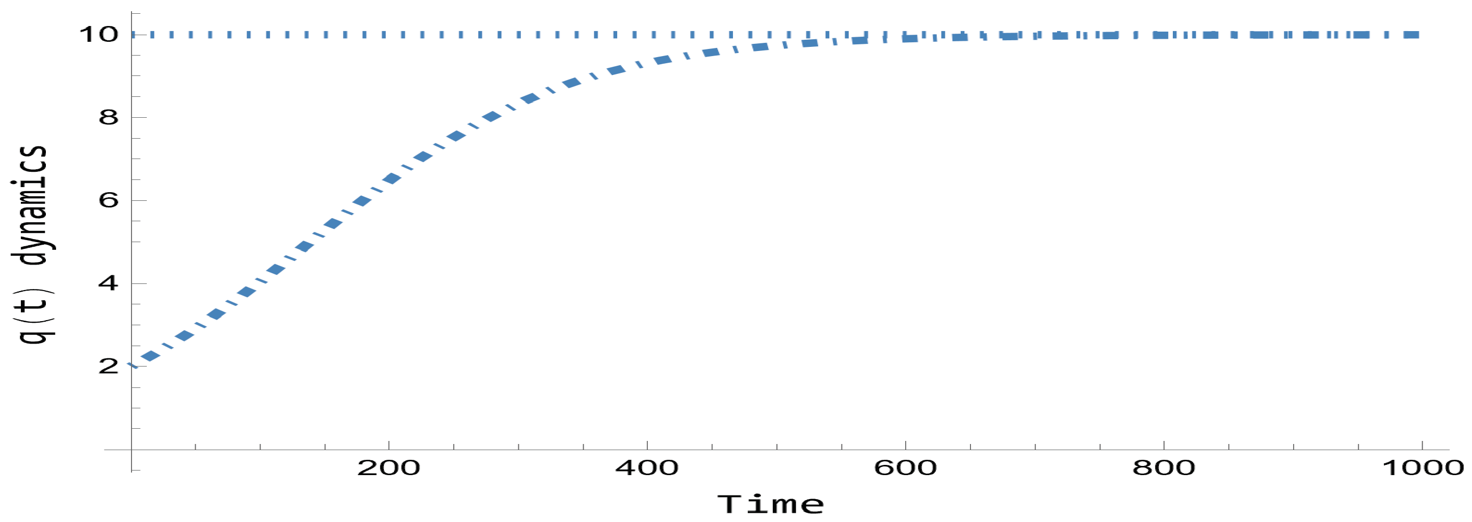
Figure 2.
(left) and the corresponding funtion (right) for the interval .
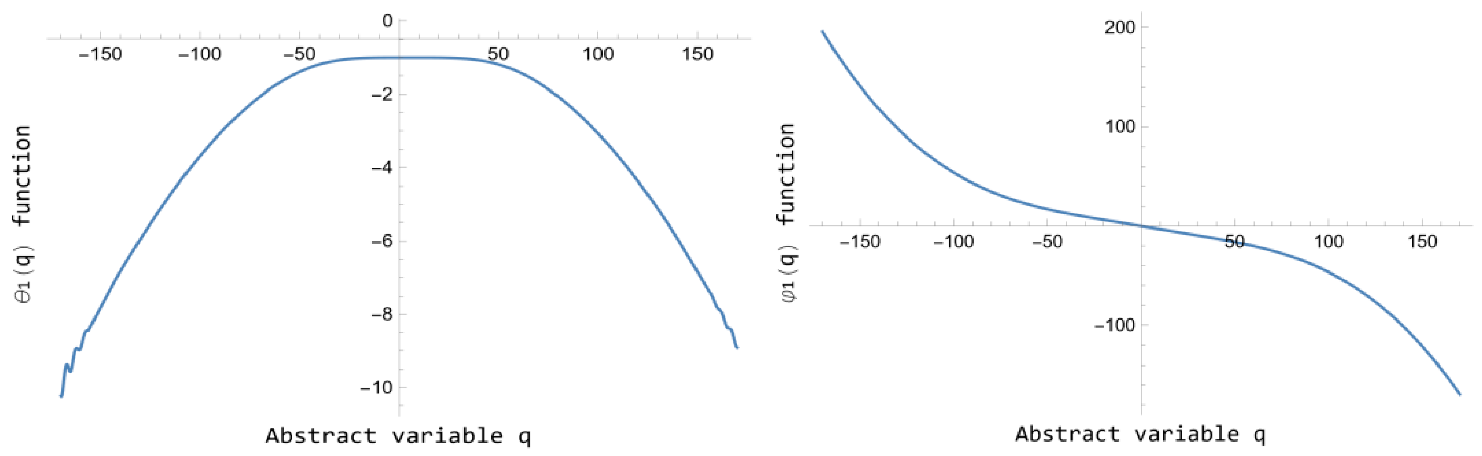
Figure 3.
Normalized wave function for (left) and the corresponding quantum dynamics for (right). The quantum dynamics corresponds to the continous curve, while the dotted straiht line value represents the saturation value and the dot dashed curve the classical logistic dynamics.
Figure 3.
Normalized wave function for (left) and the corresponding quantum dynamics for (right). The quantum dynamics corresponds to the continous curve, while the dotted straiht line value represents the saturation value and the dot dashed curve the classical logistic dynamics.
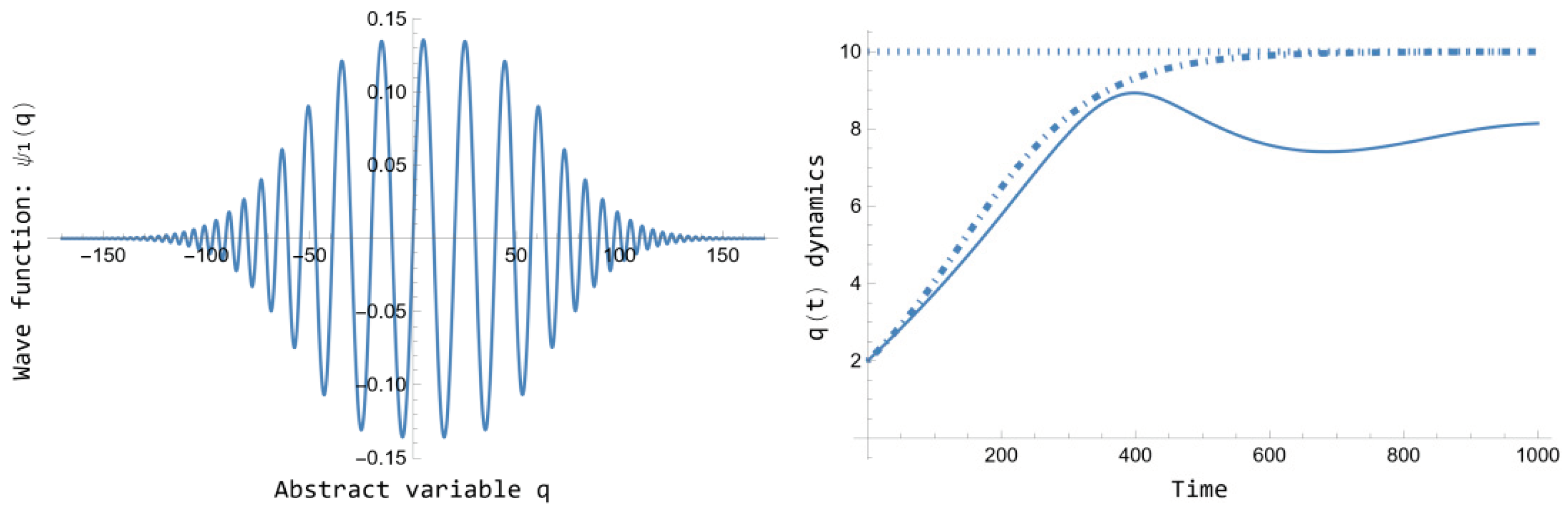
Figure 4.
Normalized wave function for (left) and the corresponding quantum dynamics for (right). The quantum dynamics corresponds to the continous curve, where the vertical line in represents the singularity, while the dotted straiht line value represents the saturation value and the dot dashed curve the classical logistic dynamics.
Figure 4.
Normalized wave function for (left) and the corresponding quantum dynamics for (right). The quantum dynamics corresponds to the continous curve, where the vertical line in represents the singularity, while the dotted straiht line value represents the saturation value and the dot dashed curve the classical logistic dynamics.
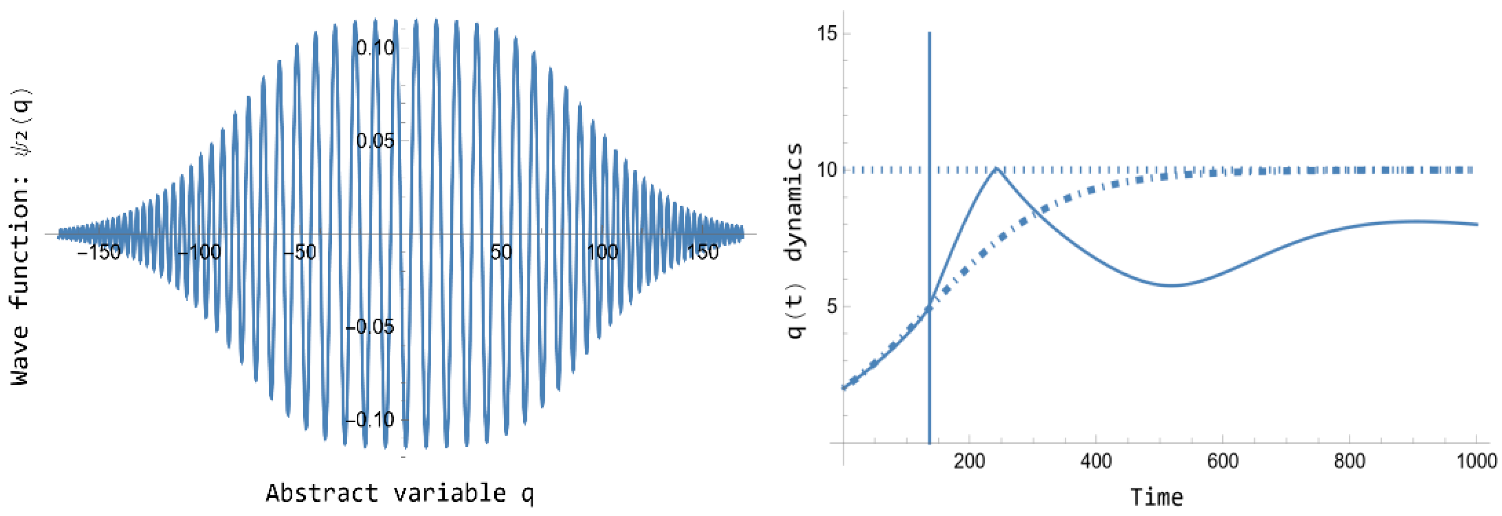
Figure 5.
Normalized wave function for (left) and the corresponding quantum dynamics for (right). The quantum dynamics corresponds to the continous curve, where the vertical line in represents the singularity, while the dotted straiht line value represents the saturation value and the dot dashed curve the classical logistic dynamics.
Figure 5.
Normalized wave function for (left) and the corresponding quantum dynamics for (right). The quantum dynamics corresponds to the continous curve, where the vertical line in represents the singularity, while the dotted straiht line value represents the saturation value and the dot dashed curve the classical logistic dynamics.
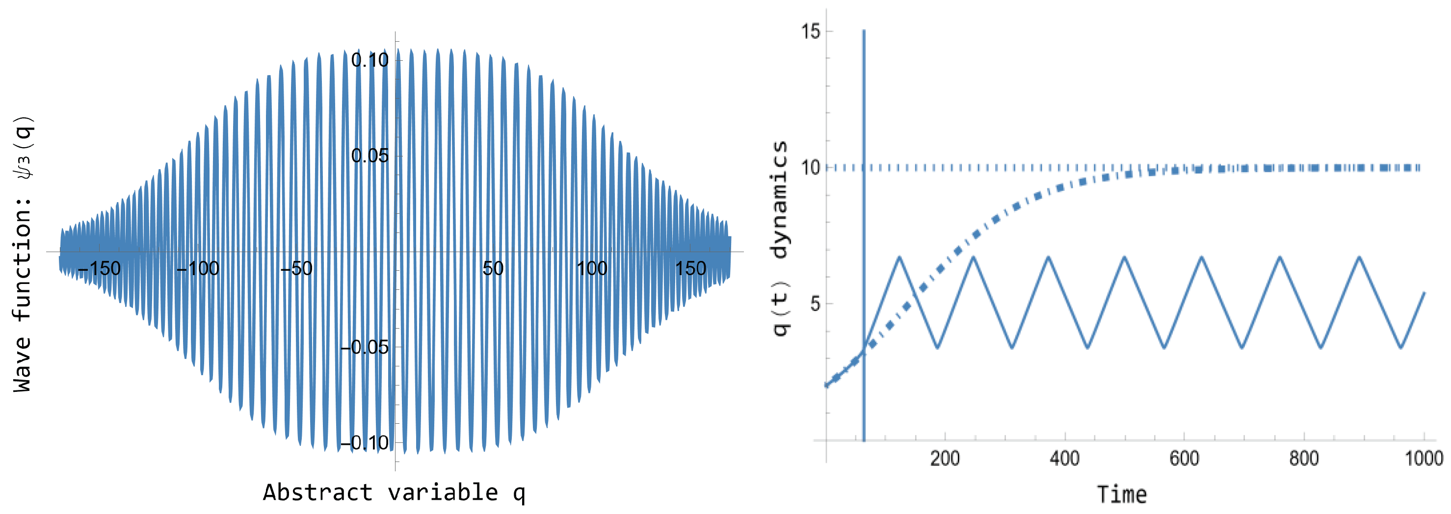

Table 1.
Quantized energies.
| n | -1 | -2 | -3 | -4 | -5 | -6 | -7 | -8 | -9 | -10 |
| 4.838 | 19.350 | 43.538 | 77.401 | 120.939 | 174.153 | 237.041 | 309.604 | 391.843 | 483.757 |
Disclaimer/Publisher’s Note: The statements, opinions and data contained in all publications are solely those of the individual author(s) and contributor(s) and not of MDPI and/or the editor(s). MDPI and/or the editor(s) disclaim responsibility for any injury to people or property resulting from any ideas, methods, instructions or products referred to in the content. |
© 2024 by the author. Licensee MDPI, Basel, Switzerland. This article is an open access article distributed under the terms and conditions of the Creative Commons Attribution (CC BY) license (https://creativecommons.org/licenses/by/4.0/).
Copyright: This open access article is published under a Creative Commons CC BY 4.0 license, which permit the free download, distribution, and reuse, provided that the author and preprint are cited in any reuse.