Submitted:
01 March 2024
Posted:
04 March 2024
Read the latest preprint version here
Abstract
A model of space-time is presented, whose origin is set before the appearance of any universe. It uses concepts of previous work, a central one being that the information about the laws of nature is stored locally everywhere in space such that all physical processes obey them. Since information storage is bound to matter or energy, space is assumed to consist of dark energy (DE), which thus assumes an importance far beyond its function as a stopgap for an energy deficit in our universe (U). The primordial state (PS) is a timeless and relatively large space of 3 dimensions described by a Wheeler DeWitt (WDW) equation, whose solution is interpreted as an arrangement of very many space quanta and possesses all the characteristics of the time-honored concept of the unmoved mover. The comparison of WDW solutions belonging to different mass densities of the DE favors one in which the space quanta are mini black holes, and allows the space quanta to be imagined as mass points that are kept at a distance compatible with the quantum volume by the Pauli principle or something equivalent. Triggered by an increase in probability, the PS is followed by a time-dependent state of space expansion (ES). The concomitant emergence of time occurs in a lightning huge crash, consuming almost all DE of the PS. The subsequent expansion proceeds in quantum leaps, whose huge size emerges from a WDW equation novelly derived from the time-dependent classical expansion solution, and is also used as size of the PS. Information is assumed to be geometrically stored in arrangements of space quanta similar to how genetic information is stored in DNA molecules. During space expansion information must be transferred from already existing "information quanta" to new ones. This requires time, slows down the expansion and is taken into account by a friction term in the cosmological momentum equation. Sinc e the Friedmann-Lemaître (FL) equation remains fully valid, the model can exclusively be based on recognized equations, so that the assumptions used to build it can be understood as interpretations.
Keywords:
space-time
; generic space expansion
; emergence of time
; dark energy
; quantum gravity
; Wheeler-de Witt-equation
; volume quantisation
; friction by information transfer
; information quantum
1. Introduction
This paper examines the model of a timeless primordial state (PS) of pure space preceding everything, the emergence of time from it, and the subsequent evolution of space-time. It results from a series of earlier investigations ([1,2,3,4,5]) each of which has provided ingredients for a new overall concept. Because it’s often about subtleties, and in order to achieve a largely self-contained presentation, some of our earlier calculations, that are important for this paper, are reproduced here (mostly in the Appendix) in compact form and adapted to the present needs. This is important also for the reason that from them partly other and partly new conclusions are drawn. Unlike the earlier studies, which dealt with the origin of , space expansion, DE, and a multiverse, this paper focuses on the origin and structure of space and time. Essential concepts on which it is based are conveyed below.
1. Already since early antiquity there has been felt a need for putting an end to the endless chain of cause and effect that makes each cause the effect of a preceding cause. For this, Aristotle proposed the concept of the unmoved mover [6], a kind of primal force which gave the impetus for all later movements in the universe without having been moved itself. In Ref. [1], an equilibrium between attractive matter and a repulsive cosmological constant or a scalar field was derived and introduced as initial state of . Because this equilibrium is unstable, the transition to a temporal evolution is triggered by disturbances. This scenario already exhibits almost all the characteristics of an unmoved mover. (The only exception could be dynamic processes in matter on microscopic scales.)
In this paper, the PS is derived by applying a WDW equation to a simple minisuperspace model. It is timeless, has only 3 spatial dimensions 1 and corresponds one hundred percent to the concept of the unmoved mover due to its complete timelessness. It turns out particularly important to formulate the WDW equation not in terms of the expansion parameter a, but of the corresponding volume , because this reveals structures which can be interpreted as space quanta. This has already been observed in Ref. [5], where the case of a PS consisting of very many space quanta was formulated as a problem. Its elaboration constitutes the content of this paper.
2. Another ingredient is the assumption that the space is uniformly curved and expands, which also pertains to concepts of e.g. Vilenkin [7,8], Linde [9], Hartle and Hawking [10] and Ref. [11]. An important reason for this is that only such a space can have come into existence at some finite time in the past, while a Euclidean space has always existed, even if it expands. Our decision for a model of this kind is also motivated by the fact that everything observed in and also itself had a beginning.
2012 it was shown by a global transformation of expanding space solutions of an FL equation, that the space expansion of can also be viewed as an explosion in a non-expanding and almost Euclidean space [2], in contrast to the general view since around 2000 at the latest. After this interpretation was initially received with skepticism, it was later devaluated as a matter of course, arguing that General Relativity (GR) would allow you to employ any coordinate system of your choice [12]. However, this argument falls short as shown by the example of a coordinate system which rigidly rotates in conformity with the earth. Already from 27.6 times the distance between earth and sun the rotation speed exceeds the speed of light, so this coordinate system is unsuitable for describing a whole universe. Another example is the coordinate system commonly used (and also employed by us) for a uniformly curved, expanding space. This space expansion cannot be transformed away globally, because the matter flowing away from the explosion site in all directions would flow back after reaching the antipodean position and collide with the flow towards the latter. 2 This means that it constitutes a generic expansion, a property that will turn out to be essential for our model.
3. In our present model, the space is uniformly filled with DE which is needed for space expansion and information storage. It thus fulfills important purposes, which have already been discussed more detailed in previous work [3,4,5]. In particular, this provides the reason why DE is even present in , observed as a gap filler for a significant energy contribution missing in the energy balance without it, and by an acceleration of ’s expansion. DE can thus be considered as a fingerprint of the space containing . In short space-time is tied to the presence of DE and would not even exist without it, i.e. DE is space energy. As in the above papers, we assume that in the PS it is due to a cosmological constant and has a huge mass density close to the Planck density.
An independent argument for our assumptions about DE is the following. Space is so slightly curved and therefore so extended that it reaches far beyond the boundaries of . According to current knowledge, within the DE is present and evenly distributed everywhere, also between the galaxies. It would be very strange if this distribution would stop at the boundary of . This consideration also led us to assume that DE is the substrate of space and gives it gravity.
4. Physics describes the elements of matter through particles and fields and their temporal behavior through interactions between them. The description of the elements comprises properties that determine which of them interact, how strong the interactions can be and what type they are. However, this description is rather simple, using just a few parameters such as rest mass, charge, spin, etc. for particles, and scalars, vectors, tensors, etc. for fields. This is by far not sufficient to determine the temporal course of interactions which is rather regulated by much more complex laws of nature that the matter elements must obey. As things stand today, this is done in a ghostly way as if following a categorical imperative [13,14]. A more scientific approach must take into account that material elements like an electron have no receiver, no brain and no power source to perceive instructions and convert them into prescribed actions.
Perhaps the most important ingredient of this work is a proposal how the obedience to all the laws of nature can be integrated into the rule book of physical description in a manageable and, as far as possible, minimally invasive way, presented for the first time in Ref. [4] and elaborated in Refs. [4,5]. The proposal was inspired by biology, where the molecules forming an animal or a plant are assigned their tasks by the genetic code written down in the DNA. Accordingly, we assume that all information about the laws of nature is encoded into submicroscopic structures of space granules (quanta) forming the timeless PS. Presumably, this will not take the form we know, but rather the form of instructions on law-conforming actions. It follows that the volume of the PS must be very large to contain the huge amount of the pertinent information. This leads to striking differences in the subsequent ES compared to the models studied in Ref. [5].
The temporal evolution following the timeless PS consists in a generic space expansion as described above (see 2.). That this is not an auxiliary mathematical construct but a real physical process has a decisive meaning for our model. Unrestrained, the huge cosmological constant would cause a strongly accelerated space expansion and thus ever faster create new space elements, to which the information about the laws of nature must be transferred from the already existing ones. This requires a fixed amount of time, while the available time becomes increasingly scarce as the rate of expansion increases. Obviously, this hinders the expansion, which we take into account in a lump sum by subtracting from the expansion acceleration a "friction force" proportional to the expansion velocity, as in our earlier work. It was left open there, how the information is stored. In this regard the present study makes a slightly more concrete proposal, which has similarities to how space quanta are arrived at in LQG, using the group properties of polyhedra and a WDW equation.
2. Basic Equations
For many calculations in this paper it is useful to be performed in dimensionless variables that refer to Planck quantities. Therefore, a section of the quantities used for this purpose and of useful relations between them is placed here in front.
2.1. Planck Quantities, Relations between Them, and Dimensionless Variables
We need the Plank-length , Plank-time , Planck-mass and Planck-mass-density :
The following relations between them are utilized:
The last one is obtained according to
Besides the dimensional quantities (essentially a radius of space curvature), time, and volume of space we use corresponding dimensionless quantities x, , and v resp., defined by
Comparing the last two relations yields
2.1.1. Approximations, Abbreviations and Numbering of Equations
In the calculations of this paper often approximations are made, which lead to extraordinarily small inaccuracies. Therefore in most of such cases = is used instead of ≈. For the readers convenience, all abbreviations are listed before the Appendices. Concerning equations, sometimes more than one appear next to each other under one number. If reference is made to one of them, the left is marked with a and the right with b in the case of two, or the middle with b and the right with c in the case of three equations.
2.2. Friedman-Lemaître Equation and Modified Cosmic Momentum Equation
Our model of space-time is based on the assumptions that the space is uniformly curved, thus closed, and uniformly filled with DE of mass density . In the framework of GR, a space-time of this kind must satisfy the (classical) FL equation
Regarding we assume as in Refs. [4,5] that the activity of the cosmological constant remains in force during the space expansion following the PS, but is impeded and thus weakened by the information transfer to the newly added space elements. As already mentioned, we take this into account by adding a friction term (linear for reasons of simplicity) in the cosmological momentum equation , which follows by time derivation from Eq (6) with , thus obtaining
where is a constant, and is the (constant) mass density of . Multiplying this equation with and integrating it with respect to t from 0 to t yields
In order to remain within the framework of recognized physics, we require that in spite of the added friction term Eq. (6) is still valid, whence or
This means that Eq. (7) implies the validity of the FL-equation (6), if the latter is satisfied for , or, in other words, the solution of Eq. (6) can be obtained from Eq. (7), if Eq. (6) is only used as an initial condition at for the latter. Inserting Eqs. (4) and using the relations (3), Eqs. (6) and (7) become
and
Eq. (9) only serves as an initial condition for Eq. (10) at , i.e., . From Eqs. (8) follows
For the system under consideration, the quantization according to the WDW method is performed at the FL equation. As already mentioned in paragraph 1. of the Introduction, we don’t do this with regard to the scale factor a as usual, but rather with regard to the volume V. Hence we still specify how the FL equation reads in terms of the volume
of a uniformly curved and closed three-dimensional space. For this purpose, we only have to insert the relation in Eq. (6) to obtain
The corresponding equation in dimensionless quantities is obtained by inserting (according to Eq. (5)) into Eq. (9) and is
2.3. Interpretation of the FL Equation with Friction Losses
Eq. (7) can also be viewed as the motion equation for a solid body of mass 1, accelerated by a force and decelerated by a frictional force . Under suitable initial conditions it can be integrated to the same energy law as that in Eqs. (8) with , i.e.
The terms on the left represent the total energy of the body, and the term on the right the accumulated friction losses, so overall there is no conservation of energy. The latter can be achieved by including the surroundings (e.g. air) of the body, where the friction losses appear as heat energy.
In our cosmological case, there is no environment to absorb energy losses, and moreover, is no kinetic energy, so the considered equation must be interpreted quite differently. For this purpose we reformulate it into
The first term on the left is the primordial rest mass density, and the second represents losses of it caused by the friction force and accumulated during the time t. The negative quantity is the energy density of the gravitational field caused by the rest mass and is reduced by the friction losses according to amount just as much as . This means that the same equation as above now implies conservation of energy as required due to the closedness of the system space as a whole. These relationships enable a simple graphical representation, as shown in Figure 1.
3. Primordial State
Because of its extremely high mass density close or equal to the Planck value , the PS of the examined space-time system must be described by a general relativistic quantum theory, in our case a WDW equation. From this follows that must be time-independent (see after Eq. (A3) of Appendix A) so that Eq. (13) reads
In Appendix A, the WDW equation (A4) with is derived from this in terms of the dimensional quantity V, and the substitution in it yields the WDW equation (A5) with ,
As in ordinary quantum mechanics, we interpret ( since is real) as a probability density, i.e.
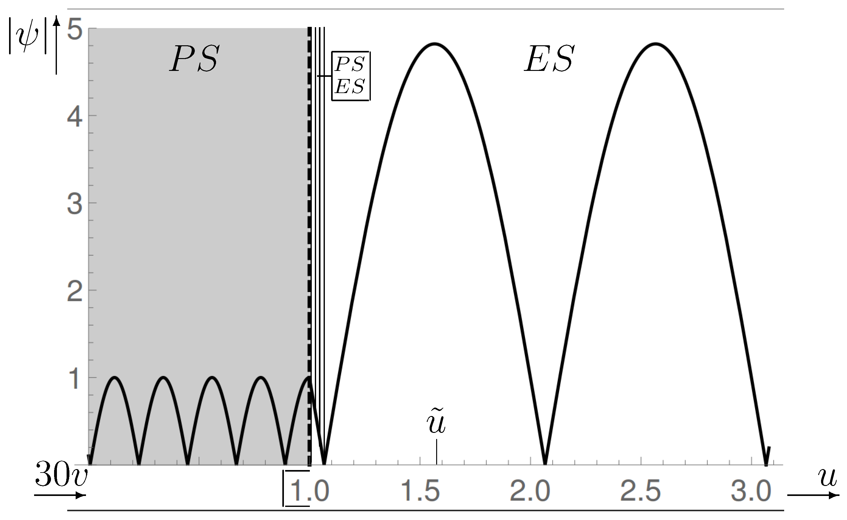
It cannot be localized at spots of one specific space, but it rather is a density with respect to contiguous volumes of independent spaces in the (virtual) ensemble (Hilbert space) of all theoretically possible spaces exhibiting the properties specified at the beginning of Section 2.2. (We come back to this interpretation in more detail in Section 5.2.2.) In Figure 2 the probability density is plotted for two solutions of Eq. (17) to small initial values and specified later in more detail. It has zeros at essentially equidistant consecutive points and nearly equal maxima close to the centers of neighboring zeros. The fact that has practically the same shape in essentially all intervals bounded by adjacent zeros constitutes a crucial point of our model: we consider in each of them as a separate quantum state in which the middle value has the highest and each edge point has zero probability. From this follows that v can only assume discrete values differing on average by , and from this it can be concluded that each of these discrete volumes consists of space quanta of average size . In principle, values from the interval would be possible for them. In order not to unnecessarily complicate our calculations, we use the most probable value in the further course. (It can be guessed, however, that refining our model – as, for example, towards the end of Section 3.1.1 – would yield sets of space quanta with slightly different sizes.)
As explained in paragraph 2. of the Introduction, the volume of the PS must be extremely large for being able to store the information about all laws of nature. In Eq. (17) the second term in parentheses can be neglected against the first for according to Eq. (33a), which is the case for almost all v, given the large size of the primordial volume we find out later. Under these circumstances, Eq. (17) simplifies to
Of the two independent solutions, a suitable one is
where for the amplitude we could arbitrarily chose the value 1, because every multiple of a solution is also a solution. The probability density has the period , from which with it follows, that
with
are the most probable volumes that the PS can assume. (For the numerical values the later result (33a) for was used.) The total volume of the PS is
where has yet to be determined. From this it can be concluded that the total volume is composed of elementary volumes whose average and also most probable size is (or in dimensionless variables). We assume that or resp. is a most probable volume between two adjacent zeros of from Eq. (20) too. We set the end point of the PS so that
For the sake of simplicity, we address or resp. as the uniform volume of space quanta in the further course. This simplification does not matter for all applications in this study, because – except for a rough determination of the primordial mass density in the next section – we always have to deal with very large numbers of space quanta, for which only their average volume matters. (This is due to the fact, that differences in size and probability, which we are actually dealing with, cancel each other out in the sum.) However, at the end of Section 3.1.1 we consider – if only qualitatively – the possibility of distinguishable space quanta that could turn out useful for the information storage so important for our model.3 Numerical values for and the corresponding extent of the PS,
are derived in Section 5.2.1. proves so large that it consists of a huge number of space quanta.
3.1. Determination of the Primordial Mass Density
From Eqs. (21) results with the definition of in Eq. (10c)
i.e. the size of the space quanta is a function of the mass density of the DE in the PS and is not fixed by the WDW quantization. However, by comparing solutions of Eq. (17) for different values we will come to a choice that is acceptable although not stringent. It appears sensible to limit our search to the range where quantum and GR phenomena are equally important, from which it follows that must be located in the region of . Accordingly, we must expect the space quanta in the PS to be tiny black holes. In the next section, we want to find out from which point on this is roughly the case. For this, we content ourselves with a simple calculation, ignoring both quantum and GR effects. We then numerically determine the solution of Eq. (17) for different values of or resp. and decide which one seems most suitable for our purposes. The preceding rough calculation will help us to get a particularly illustrative picture of the space quanta.
3.1.1. Simple Black Hole Model
Not only for the simple model now considered, but in general we assume that the whole mass of space is contained within the space quanta .
In the following more detailed calculations we restrict ourselves to space quanta forming non-rotating black holes and consider the entry point of black holes, at which the radius of a sphere of homogeneous mass density (, see Eq. (30)) just coincides with the Schwarzschild radius
where is a constant yet to be determined. From this follows with Eqs. (1) and (2)
and with this the volume of the considered Schwarzschild sphere becomes
We assume that the Schwarzschild spheres of our black hole quanta do not penetrate each other, but touch in points and arrange themselves in the closest packing possible, the one claiming the smallest total volume. According to Ref. [15], this means that the individual spheres occupy the part
of the the quantum volume from Eq. (21), found without assumptions about the shape. Substituting the non-numerical part of Eq. (21b) and Eq. (27) into Eq. (28) and solving for yields
Under the natural assumption that there is only one black hole in each space quantum of volume , the primordial mass density is
Inserting into this obtained by resolution from Eq. (10c), from Eqs. (21), from Eq. (26), and from Eq. (3), we obtain
and substituting this into Eq. (29) finally yields
With this, we get from Eq. (31) and Eq. (10c)
The fact that is only about 1 percent of indicates that our classical calculation for the mini black holes is not too wide of the mark. A numerical solution of Eq. (17) for this is shown (Figure 2) and discussed in the next section.
Besides the spherical black holes considered so far there are also rotating black holes. This opens the possibility to include space quanta with spin, that can have slightly different volumes (which is useful because our model allows for space quanta with different volumes). For massive objects with spin the quantum rules are well known and could be used for a different kind of loop quantum gravity (LQG) in a similar way as the polyhedra for the usual LQG [16,17]. In particular, space quanta with equal spin but different spin orientations could provide an alphabet for information storage.
3.1.2. Solutions of the WDW Equation for Different Values
When solving Eq. (17) numerically, we want to exclude the case of a space with vanishing volume and would therefore prefer initial conditions such that and vanish for . However, instead of zero, we have to take a very small value for v (we chose ) in order to avoid becoming singular. must also assume a value in order not to get the solution . Furthermore, we want to obtain solution (20) for large values of v. For this purpose, the initial value of was chosen so that for large v (about 20 times the largest v in each picture of Figure 2 and Figure 3) the amplitude of is 1.
In Figure 2, the left picture shows the solution for or obtained in Eq. (32) of the last section. The dashed vertical line marks the volume , which would result if the space consisting of a single space quantum had the volume of space quanta derived for large v. The horizontal line represents the amplitude of the asymptotic solution (20). For larger v there is already good agreement. That there appear increasing deviations with decreasing v is due to the fact that simultaneously the space curvature becomes more and more noticeable. According to our model the PS does not arise from a growth process, but by definition consists of a huge number of space quanta. This means that the differently shaped states of small v do not appear at all in a PS with many states. (It should be remembered that the solutions do not represent one, but many spaces of different sizes.) Rather, we can assume that all space quanta have the same volume from Eq. (21) that applies to very large v values.
Even though we have seen that the deviations from the asymptotic behavior that occur at small v do not play a role for a large PS, one will prefer if the space quanta in small spaces are approximately the same as in large spaces. This certainly does not apply to the case shown on the left in Figure 2 due to the large gap of about between and the v belonging to the first maximum of . For this reason, we have examined a number of other cases which show that the situation improves with increasing or resp. The right picture in Figure 2 shows the situation for ten times the value of as in the left picture. The first quantum state still has slightly more than twice the volume . In Figure 3, is again magnified by almost a factor of 10 to . This situation is already almost optimal, and it has turned out that further enlargements (up to ) do not result in a complete agreement with . We have therefore decided on the case
for all further calculations, which indeed represents a compromise. Since the value is almost 100 times larger than the value at which, according to our rough calculation in Section 3.1.1, the space quanta just become black holes, we can assume with considerable certainty that the space quanta, which we ended up with, are indeed black holes. According to classical GR it follows from this that they are mass points. Nevertheless, each of them requires the finite volume . This does not imply that they have a structure, but simply means that they must be spaced apart according to their volumes. However, in correspondence to the classical rotation of black holes, they can still have a spin, which is relatively easy to handle quantum mechanically.
In Table 1 the values of , and are listed for the solutions represented in Figure 2 and Figure 3 and for volume quanta obtained in the LQG [16]. The value of corresponding to the latter is calculated with Eq. (25).
Given the uncertainties associated with each of the underlying assumptions, the results reported in the Table are fairly consistent.
4. Evolution of Space-Time, Classic Treatment
When calculating classical quantities, we can leave it with the usual dependence on x instead of v, because wherever necessary we can use to switch to the v-dependent representation, without changing anything conceptually as with the derivation of a WDW equation.
The classical evolution of space-time can be completely described by the solution of Eq. (10) to the boundary conditions (A7) and (A8), according to Eq. (A6) with Eqs. (A9) of Appendix B given by
After Section 2.2, at this the FL equation (9) is already fully taken into account. With , according to Eq. (33), and in anticipation of the later results (51), , and (86), , instead of Eq. (34) we can use with extremely little error the much simpler representation
where the upper sign, −, holds for . The comparison of the two bracketed terms yields
from which follows that due to the extreme smallness of we can write with extremely high accuracy
4.1. Determination of and
Although Eq. (9) must no longer be taken into account, we can still use it to calculate or resp., i.e.
If we were to use Eq. (36) for calculating , according to Eqs. (9b) and (37) the initial value of in the ES would be which contradicts Eqs. (11a) and (33b). In order to remove this discrepancy, for calculating we must instead employ Eq. (35) to get
With Eq. (36) and the (very precise) approximation follows from this
so we finally get
With this result the discrepancy disappears, because for , neglecting and versus (based on Eqs. (33a), (51) and Eq. (86b)), we get and from Eqs. (9b) and (10c) as required. For sufficiently large values of , the second bracket term in Eq. (40) becomes negligible versus , and we obtain
To find out more precisely when this is the case, we determine when or holds. This is the case for
with
where Eqs. (1), (4), (33) and (51) were used for the numerical values. After just Planck times or seconds resp., i.e. practically instantaneously decreases from the huge value to the much smaller value
(coming about due to ). This density decrease without equal represents a practically instantaneous and exorbitantly huge crash. Detailed reasons for its occurrence are discussed further down. It is particularly noteworthy that due to the collapse of the density leads almost exactly towards the density that results from the FL equation (9) for the equilibrium at . The solution belonging to (lower sign) even leads exactly to this point, because Eq. (38) results in
In relation to our model, however, this is not an equilibrium, because from Eq. (10) follows for . Because the solutions for both signs behave essentially the same, we further on restrict ourselves to that with the upper sign, i.e. .
We can now use Eqs. (9b) and (41) to calculate by inserting for today’s value and resolving for ,
where is the present value of . Since in , DE contributes 68.3 percent of the total mass density and the latter equals the critical density with present Hubble parameter and present Hubble time, we have
Here, was plugged in, a value that is slightly higher than the age of , but slightly below the last values obtained from measurements for . (This value was chosen because it yields a particularly handy result for .) The value of can be freely specified, but only above due to Eq. (46). For illustration we relate it to the radius (slightly below present the Hubble radius ) by setting or
Inserting all this into Eq. (46), we get with
from which the condition
results for obtaining real values of . For the space curvature to be below the maximum value compatible with measurements, according to Ref. [18] the condition must be satisfied. In Appendix D it is shown, that in terms of our parameters this amounts to . In , the DE is usually attributed to a cosmological constant. Since the DE of our model fills up the entire space and thus also that of , it should share this attribute, so we assume that at least during ’s present lifetime the density of the DE is largely constant. For this reason we choose still well above 14.5. The value seems sufficient to us and shall serve as a reference value. With this, due to , we get from Eq. (49) with very little error
With the specification of now also can be calculated. According to Eqs. (9b), (36) and (41) the further evolution of the density after its crash (i.e. for ) is given by
Characteristic values, calculated with this, Eqs. (33), (48), (86), (89) and are given in Table 2.
We are additionally interested in how the expansion rate changes over time t. For this we first calculate and for some times . From Eqs. (36), (39), (51) and (86) we get
and
where the relation , used for defining , was employed to calculate . For Eq. (36) can be used for calculating , and together with the above relationships, Eq. (59a), and for , we get the values given in Table 3.
The values corresponding to are obtained from
so simply by multiplying by the speed of light.
4.2. Causes of the Density Crash and Disequilibrium of the Initial ES
The causes of the initial density crash can best be understood on the basis of Eq. (37). The values of the quantities on the right before and after the crash are given in Eqs. (53) and (54) resp. must even be larger than the already rather large extent of the PS (consisting of very many space quanta according to Eq. (97)) in order that can assume the high primordial value . (If it consisted of only one or a few space quanta, would be almost zero, and then the term in Eq. (37) would provide the required high density.) From Eqs. (53) and (54) follows that essentially whereas , i.e. changes virtually not at all during the crash, while changes by almost 62 orders of magnitude. In short, the huge extent of the PS in combination with the large initial value of requires a large initial value of (see Eq. (9a)), but both are pushed down nearly instantaneously by many orders of magnitude, by 42 (see Table 2) and by almost 62 (see Table 3).
The reason for the latter arises from Eqs. (10b) and (A6b). Solving the latter with respect to and taking advantage of the smallness of gamma we obtain
The high value of this friction coefficient combined with the high velocity leads to the extreme friction force
against which the force
can easily be neglected. Eq. (10) thus results in
The extremely fast change of at leads there as expected to an extreme curvature of which looks like a kink (see Figure 5).
The extremely high initial velocity in the initial state of the ES means that the space is in an extreme disequilibrium. Obviously, this affects the density much worse than an instability, where first a velocity or must gradually be built up. Now, from a classical point of view, the initial ES is the same as the PS, and one might assume that the latter is also in a disequilibrium and therefore decays. In the PS, however, time does not even exist, and hence the question of equilibrium or disequilibrium is irrelevant. Even so, we will see later that the density crash, initiated by the emergence of time, affects the state of the ES in such a way that an increased probability for the quantum mechanical transition from the PS to the ES comes about.
4.3. Age of Space-Time and Constancy of during U’s Lifetime
To determine the age of space-time, we first obtain from Eq. (36)
With this and Eqs. (1), (48) and (86) we get for the present age of space-time
For the reference value follows from this
where
is the age of .
Now we pursue the question of how it is about the required constancy of during the lifetime of . For this, using
we first go in Eq. (36) from to a larger time scale in which the age of becomes . In this way we obtain from Eqs. (9b) and (41) with Eq. (36)
where for the numerical evaluation Eqs. (51), (59)–(61) and (86b) were used. If future measurements should show that the per mil decrease in found herewith is too much (or too little), our reference value of could accordingly be adapted.
4.3.1. Universality of t, Irreversibility and Causal Connection
As in the theory of U’s expansion, the time of our model is a measure of change. The mass density of the DE is a monotonically decreasing function of t and thus provides the changes necessary to define a time. From the time after the end of the density crash on, or resp. is given by Eqs. (9b) and (41). Substituting from Eq. (36) and solving for yields with Eqs. (4) and (9b)
is distinguished by the fact that it can be understood as a universal time, which can even be applied to different parallel universes. It is related to the coordinate system used in our model and can physically be characterized by the fact that in it, the DE density has the same value everywhere at any fixed time t.
Due to the friction term in Eq. (7), the passage of time becomes irreversible, time is given an arrow in the forward direction. However, there is no major difference to the course of time in a universe described by reversible equations, which in many models also runs just in one direction without reversing. The only difference is that in our model, there is no solution traversing the same states backwards in time. Further below in Section 6.2.1, we still take a closer look at the problem of irreversibility.
Table 3 shows that the present expansion velocity of space is times the velocity of light. This makes it interesting to look at the observation horizon of space, given by
What is of most interest here is its relationship to the radial distance
which leads from a starting point to its antipode. For calculating the ratio we use , , and (according to Eqs. (51) and (59)) and obtain
This means that from a fairly short time on, all space is causally connected. This result is of some relevance to the issue of whether traces of the existence of earlier and, like ours, expanding universes can be detected in . For this it may matter that the space expansion of a universe can also be interpreted as an explosion [2], whereby its boundary moves almost at the speed of light. That the boundaries of two universes are consequently approaching each other at a higher speed will however only apply to relatively neighboring universes, because the ever faster expansion of space is a genuine space expansion that can only locally be transformed away. This shows again how important it is that the space expansion in our model is genuine, because without it the explosive propagation of universes would have long since led to unmissable collisions between and other universes.
5. Evolution of Space-Time, Quantum Treatment
The ES starts deep in the quantum regime, which is why one would like to have a WDW equation available for it as well. However, because is time dependent in the ES, one cannot proceed as usual. Even so, we have found a way to get around this difficulty by using the fact that we already know the classic solution . By substituting its inverses into and using one obtains the function , inserts it into the FL equation and can then derive the associated WDW equation as usual. In its solution we separately treat the short transition from timeless to time-dependent associated with the density crash and the subsequent long-lasting evolution until today.
A WDW equation for the ES that includes both the period of the density crash and the subsequent time of the space expansion is derived in Appendix C and is
The initial conditions to be satisfied by solutions are continuity of and in the transition from PS to ES at , i.e. Eq. (23),
The reasons leading to the density crash also cause extremely rapid changes in which provide considerable difficulties for a numerical solution. The latter is unavoidable because there are no analytical solutions. Some reduction in difficulty is achieved by changing from the volume v to the relative volume
( being defined in Eq. (22) and calculated in Eq. (86)) by which Eq. (64) is transformed into
and the initial conditions (65) become
(Note that describes the same physical object as but is not the same mathematical function.)
5.1. Decomposition of the Wave Function into Branches
Based on numerical results obtained for (relatively) small values and shown in Figure 4, we now seek a solution to this equation for the extremely large true value, considering two branches: one, the main or residual branch, with values of large enough for neglecting the term against 1 in Eq (67), and another, the initial branch, with values of so small that is practically indistinguishable from its initial value .
5.1.1. Main Branch
The condition to be imposed on the main branch is fulfilled if
applies for sufficiently large . Now
where the e-function was expanded into a Taylor series that could be truncated after the second term because of , due to the extremely large value of without noticeable error. In summary, the condition is
In particular, we get
The solution of the equation
obtained by omitting the term in Eq (67), can be represented in the form
where the coefficients A and still need to be determined.
5.1.2. Initial Branch
We now turn to the initial branch, extending from to . Because the point of attachment to the main branch is so extremely close to , as verified later, we can assume that up to it, is practically indistinguishable from its initial value . Under this assumption Eq. (67) can be integrated with respect to u, and with use of the initial condition we get
Executing the integration yields
Neglecting 1 against and inserting the result in Eq. (73) yields
Owing to the extremely large exponents in and we still perform the expansions
in the exponent, where was used in the last step as a very accurate approximation for the extremely small values . With this and with from Eq. (69), at we get
Due to and resp. in the denominator, the first and third term between the brackets can be omitted without noticeable loss of accuracy, so we finally obtain
where at last was omitted, since and for all .
It still remains to show that our above assumption for is justified. From for according to Eq. (73) and according to Eq. (68a) it follows . From Eq. (73) it also follows that
Integrating this inequality and using Eq. (76) together with results in
and inserting from Eq. (70) we finally get for the initial branch
i.e. we have with vanishingly small error
According to Eqs. (66), (70) and (83a), the volume of the initial branch is
so negligibly small.
5.1.3. Connecting Initial and Main Branch of
The demand for continuity of function and derivative at the junction , i.e. and , yields with the results obtained in Eqs. (72) and (78) the relations
where in the sine and cosine was replaced by 1, due to Eq. (70) with vanishingly small error. From these, elementary calculations lead to
With this and Eqs. (66), (70), (72) and (86) results for the solution of Eq. (64)
valid for all . (The value of follows directly from Eq. (64) with the term being neglected, i.e. from .) As in the PS, so in the ES the square of the wave function (81) is used for calculating probabilities. For the reason of clarity instead of is shown in Figure 5 for a combination of the ES wave function (81) and the last part of the PS wave function (20).
Figure 5.
for the wave functions of the PS and Es, for reasons of visibility as a function of in the PS and of u in the Es. In addition, is plotted instead of so that the transition from PS to ES is easier to recognize. The beginning of in the ES, that looks like a short piece of a straight line, is actually a piece of the function (72) and is connected to the function of the PS at continuously and with continuous derivative. In the main text it is called appendage branch and treated in a separate section.
5.1.4. Appendage Branch
Between and (or the corresponding values of ) there is still a short branch of the wave function Eq. (72) (or Eq. (81)), which leads from 1 to 0 and at first glance may look like a superfluous appendage. It only occurs once, because we consider the subsequent arcs of the cosine function, running between two neighboring zeros of , as separate quantum states. We assume that like the subsequent ES quantum states, it did not arise from nothing. In consequence it also belonged to the PS, but like the other ES states with a correspondingly smaller amplitude, much smaller mass density and with an independent volume that was not duplicated in the transition to the ES. In this sense, it therefore belongs to both the PS and the ES and is accordingly entered in Figure 5. The size of its volume is
In fact, this branch is not at all superfluous, because from the last section it is clear that through it the amplitude A of the ES wave function and thus the probability of the quantum states of the ES (see Section 5.2.2) is enhanced. However, the space quanta it contains can also be useful for other purposes where it is not important that they are not reproduced. One possibility is that certain fractions of them have merged and survived the density crash as somewhat larger black holes. If there are enough of them, some could later appear in just emerging universes and by sucking up matter grow to bigger ones. Another, even more speculative possibility would be that other parts could form into structures that serve as seeds for the creation of universes.
5.2. Properties of the Main Solution Branch
5.2.1. Volume Increase in Quantum Leaps
The period of , i.e. the distance from one of its maxima to the next ( = half period of ) results from and is
This result means that the volume v increases discontinuously in leaps of size . In fact, as in the case of the volume quanta (or ), quantum leaps of somewhat smaller or larger sizes are possible, if only with lower probability. However, because this would unnecessarily complicate the subsequent discussion of information transfer, we assume that the leaps are all the same size. Later results involving many leaps do not result in errors caused by this simplification because corresponding differences cancel by averaging. On the other hand, the possibility of different sizes even turns out to be advantageous for the individual processes of information transmission (see Section 5.2.4). The maxima of are at
in the middle between the zeroes, where
is the position of the first maximum (see Figure 5).
The quantum states of the ES extend over the volume regions , the width of which is so much greater than the width of the PS quantum states, that they must have a different interpretation. Furthermore, for our concept of information transfer to make sense, the volumes added to the ES with each quantum leap must contain the same information as the PS. To this end, it seems reasonable to assume that they contain the same number of space and information quanta as the PS. It is then only logical to assume that the PS has the same volume as the gradual increases in volume of the ES. Unlike in the case of the PS, each quantum state of the ES does not describe one single space quantum, but very many. Albeit, from the shape of no conclusions can be drawn about how the individual quanta are distributed in space. What we will to do, however, is draw conclusions about the probabilities of the quantum states. The assumptions just made are crucial to our model. Briefly summarized they are: The PS and the space added with each quantum leap of the ES have the same volume and contain the same number of space and information quanta.
According to the above, the quantities and defined in Eq. (22) have the values
or, after using Eqs. (4) and (1),
Expressed in multiples of the Bohr radius we have
The relative size of the volume leaps is
according to Eqs. (5) and (36). Starting from the initial value 1 deep in the quantum regime, it continually decreases, due to the small value of very slowly but nevertheless exponentially, until it disappears for . This is a paradigm of how quantum effects lose significance in the progression of the ES from the quantum to the classic regime without any approximations being made.
For the time that elapses between neighboring quantum states and is used to transfer information from already existing to newly added volume elements, we obtain from Eqs. (4), (58) with Eq. (83), and
Denoting the time elapsed until the first volume doubling with , we obtain from this with , or and according to Eq. (60)
For and according to Eq. (48), the current expansion parameter is , and with this we get
5.2.2. Probabilities
The overall wave function of space-time is composed of three piecewise solutions of the WDW equation that are continuously and with continuous derivatives interconnected: essentially Eq. (20) for the PS, Eqs. (78) for the the density crash, and Eq. (81) for the remaining ES. The value of a multiplicative factor, free in the determination of and (in Eq. (20)) deliberately set to get , can be left at its arbitrary value, because we only want to compare different contributions to the total probability, where it cancels. In our simplified determination of the quantum states by means of the respective maxima of between successive zeroes, we obtain for the ratio of the probabilities according to Eqs. (18), (20) with and (81), (84) with
where is (up to the said factor) the probability of the first quantum state of the ES, and (up to the same factor) the probability of the PS. If the amplitude of the (periodic) wave functions in the PS and ES were the same, would result instead.
In the case of variable quantum leap sizes, one would (with and ) assign the probability
to the first quantum state of the ES and compare it with the probability of the PS. Because the volume used for calculating contains all space quanta duplicated from quanta of the PS for the information transfer, we must likewise include the volume of the total PS when calculating . For this purpose, we first calculate the total probability of a single space quantum of the PS, for which with use of Eqs. (20) and (21) we get
The desired overall probability is obtained by multiplying by the total number of space quanta of the PS, given in Eq. (97), and is
This together with Eq. (92) results in
the same result as in Eq. (91).
The results (91) and (95) show that the transition from the PS with via the density crash to the first quantum state of the ES leads to a significantly higher probability. The cause is the density crash, which according to Eq. (78) leaves the value of the wave function unchanged, , but influences its further course (Eq. (72) with Eq. (80)) in such a way that either Eq. (91) or Eq. (95) becomes valid. This also influences the slope and thus the importance of the appendage branch of : the steeper the drop, the larger the maximum of .
In analogy to Eq. (91) the probability of the (simplified) n-th quantum state in the ES is (up to the irrelevant factor mentioned) , i.e. the same for all quantum states, whereas an increase with time would be indicated. The latter can be achieved by relating not to the volume but to the time with and . With this we get
so an increase with time, that plotted over v follows a step-like curve with slope .
5.2.3. Merger of Quantum States with Classical Time Evolution
The time-independence of wave functions for an entire universe (or space-time in our case) raises considerable difficulties, both in finding suitable ones and in interpreting them, particularly in view of the observed time evolution of [19]. A so-called minisuperspace model has been studied to a special extent [10], where the wave function depends only on the scale parameter a and a scalar function representing matter or energy resp. From the corresponding WDW equation solutions for a ground state of lowest excitation and states of higher excitation are derived, whereby semi-classical considerations are used for the boundary conditions to be imposed. Due to the vanishment of the total energy it is difficult to specify more precisely what is meant by excitation, but need not interest us further here.
Our model for pure space-time can also be classified into this scheme, with the important difference that we use the volume V instead of a. This difference leads to the fact that instead of the emergence of a universe from nothing as the ground state (see Figure 4 of Ref. [10] for a numerical and Eq. (101) of Ref. [5] for an analytical solution) we get the timeless primordial state PS consisting of many space quanta. The deeper reason for this marked difference is that the order of the processes of transformation from a to in the FL equation and the derivation of the associated WDW equation are not convertible. Because in Ref. [10] a wave function is searched which describes the universe we observe, it is concluded that "our Universe does not correspond to the ground state of the simple minisuperspace model but to an excited state". The latter is calculated for a universe with radiation and a cosmological constant. Accordingly, our solution (81) for the ES after the density crash can also be regarded as an excitation state, although it is derived in a completely different way and applied to a different physical situation. Furthermore, because it comes from quantization of a classical solution, it is also semiclassical. Unlike in Ref. [10], however, we do not give up our ground state but connect it continuously and with continuous derivative to our solution for the ES.
Let us now turn to the (interpretation) problem of how time-independent solutions of the WDW equation can be related to temporal evolution. A solution was already given by DeWitt [20] in 1967. With reference to this, Linde writes on page 198 of Ref. [21], somewhat simplifying, that is separated into two parts, a macroscopic observer with a clock, and the rest. Both parts can evolve in time according to the observer’s clock, but together they build the timeless universe. On page 1136 of Ref. [20] DeWitt separates the world into three parts. The material content of is one of them and can be seen "as a clock for determining the dynamical behavior of the world geometry". The latter is precisely the way in which time comes into play for the quantum states (81) associated to the volumes of Eq. (84), which in turn are associated to the densities obtained from Eq. (52). With this it finally results from Eq. (63) that the quantum states under consideration occur at times . Because Eq. (63) follows from the classical Eqs. (36) and (52), we can say that our description of the ES is an equal side by side combination of classic and quantum solutions (certainly not complementary).
Let us still briefly pursue the question of what properties a QG model must have in order to enable the transition from a ground state, e.g. our timeless PS, to a time-dependent ES. For this, the system under consideration must in addition to the quantities describing its geometry (e.g. the scale parameter a) still contain another parameter that can be used to describe changes of state. In earlier papers employing a WKB method for finding approximate quantum mechanical solutions, this parameter is an imaginary time interpreted as a space coordinate, whose continuous shift leads from imaginary via zero to real values and thus to a temporal evolution. In the WDW approach, often a scalar function is used, which e.g. is intended to describe a matter field and is quantized just like geometric parameters. In our case, where takes on the role of the additional parameter, the latter is not possible, because that part of which comes from the friction term and is essential for our model, would be treated inadequately. The new path we took to quantize the ES was therefore inevitable.
5.2.4. Cloning of Space and Information Quanta
We assume that the information about the laws of nature is geometrically stored in finite, but microscopically small bundles of partially distinguishable space quanta, which can be understood as information quanta.4The equality of the volume leaps means that they all contain the same number of space and information quanta, and that each one of them is duplicated, or, in other words, cloned during one volume leap. An immediate consequence is that the volume of the space quanta does not change in time. On the other hand, their mass is like monotonically decreasing, which means that the space quanta have both time-varying and time-invariant properties.
Note that cloning does not necessarily create just one coherent area of new space. This would only be the case if the volume added by one quantum leap would contain only one information quantum. If there were several, they would be scattered all over the already existing space, which also applies to the constructs contained in the appendage branch. According to Eq. (101) the production rate of new space quanta is constant, which agrees well with the assumption that we are dealing with a cloning process that occurs with constant probability.
Little can be said about the size of the volume which contains the information about all primary laws of nature. Due to their complexity must contain very many space quanta. However, from our assumption, that all information is transmitted during one quantum leap, it follows that . If is slightly smaller than , with relatively small integer n must hold. Thus in short we can put on record . In the case with the quantum leaps of the ES volume can have different sizes, namely with , and their description by an extended wave function makes different sizes possible.
5.2.5. Number of Space Quanta
The number of space quanta contained in the volume of the PS results from Eqs. (21) and (86) and is
According to our model, this number (or a not much smaller fraction with ) must suffice to contain the entire information about all primary laws of nature. For the present total number of volume quanta of the ES, Eqs. (83) and (104) yield
and the present number of space quanta is
For the time evolution of the number of space quanta we obtain from Eqs. (4), (5), (36) and (97)
and
5.2.6. Mass of Space Quanta and Total Mass of Space
Resulting from Eq. (21) and the mass densities given in Table 2, the mass of space quanta at various times t is listed in Table 4.
For comparison, the current upper limit of the neutrino mass (15. February 2022, see Ref. [22]) is .
For the total mass of space in the PS we get with Eqs. (32b) and (87a)
where is the mass of the sun and is the mass of the milky way [23]. (The corresponding energy is ). The total mass at the time immediately after the density crash is
where is taken from Table 2. Using Eqs. (1), (4), (47), ,
and Eq. (48), we get for the present total mass of space
For and thus we get with Eqs. (4c) and (52a)
For later purposes, in analogy to Eq. (62) we still calculate, by how much the total mass changes during the lifetime of . Using Eq. (62) first and then Eqs. (5), (36) and Eq. (61), we obtain
and finally
5.2.7. Entanglement of the Emergence of Time and the Density Crash
Mathematically, the (initial) density crash seems to be due to the (much later) extremely low present value of the DE density. This almost looks like a reversal of cause and effect, which is of course unacceptable. Conversely, a reason for the initial density drop should explain the low present value. An important hint for this is given by the equation from Table 2, by which the present DE density can be represented and from which its small value results. According to Eqs. (56) and (57), regardless of the present density a rather small value of is necessary for a large density drop, and according to Section 5.1 and Section 5.2.2, the latter is in turn the prerequisite for the high probability of the transition PS→ES and the associated emergence of time. The latter is therefore the cause of the small value of .
A comparison of the masses and given in Eqs. (102) and (103), or the corresponding energies shows that for the birth of time almost the entire DE energy as well as the corresponding (negative) gravitational energy of the PS must be spent. Due to its intrinsic entanglement with the density crash and because the latter occurs so incredibly fast, the birth of the time can truly be called a plunge birth. (This spectacular event represents an essential difference to other models (e.g. Refs. [7,8,9,10]), in which this transition is accomplished without any physical conspicuousness.)
We still want to find out if the birth of time, called emergence above, is an emergence in a scientific sense as used in system theory, philosophy or various natural sciences [24]. For this purpose we use the following definition: Emergence means that a system of many (same or different) elements has properties that are based on cooperation of the elements and which can either 1. principally not, or 2. not without knowledge of the system properties, be traced back to properties of the individual elements. Case 1 is called strong and case 2 weak emergence.
In our model, the system is space-time, and its elements are space quanta, which are treated as same in this paper for simplicity, but because of our assumption about the storage of information should consist of groups with mutually different properties. Observable system properties appear only after the entry of time or after the density crash resp., because unlike the big bang of , the big crash of our model leaves no measurable traces. From a theoretical point of view, however, the crash is an important system property, which can be traced back to a cumulative effect of the many space quanta of the PS: According to Section 5.1 and Section 5.2.2, the density crash, needed for the occurrence of time, can only come about by the fact that the PS contains extremely many space quanta and thus a very high energy , whose conservation at the transition PS→ES (i.e. and ) requires an extremely high initial expansion velocity or resp. for providing the energy to be spent in the crash. From this it becomes evident that the density crash represents weak emergence. On the other hand, the appearance of time as a fourth variable in addition to the three spatial coordinates can surely be classified as strong emergence. However, exclusively restricted to (in principle) provable properties, the system reduces to the branch of space-time or even , starting with the much smaller density or , and time is an integral part of the system from the outset and thus not emergent.
5.2.8. Schwarzschild Radii
We now address the question of how the Schwarzschild radii of the space quanta change over time. To this end, at first we slightly reshape Eq. (26) using one of the relations (3),
With this, and Eq. (21) we obtain
Typical values of this quantity are listed in Table 5.
In the PS with over space quanta, the space curvature is already so small that we can calculate the radius of a sphere of volume with the Euclidean formula, yielding
This is significantly smaller than the Schwarzschild radius , so our assumption that the space quanta in the PS are mini black holes, whose mass is concentrated in one point, is justified. We assume that the view of space quanta as point masses also applies after the density crash, even if the Schwarzschild radii are then much smaller, because there is no reason for the mass to disperse, but also because concepts with lengths wouldn’t make sense.
6. Applications and Open Problems
6.1. Mach’s Principle
Since in our model space itself has mass, it is interesting to find out about the validity of Mach’s principle. The latter received its name from Einstein in 1918 and states a relativity of inertia. More precisely it says "that the inertial forces experienced by a body in nonuniform motion are determined by the quantity and distribution of matter in the universe" [25]. Einstein was not insignificantly influenced by this principle during his work on GR and was for some time even strongly convinced of its validity. Later, however, he distanced himself from it because doubts arose about its general validity. According to Abraham Pais [26], ”after Einstein, the Mach principle faded but never died. … at stake is … whether a theory is then acceptable only if it incorporates this principle as a fundamental requirement (as Einstein had in mind 1918), or whether this principle should be a criterion for the selection of solutions within a theory, that also has non-Machian solutions.”5In our model, the behavior of material particles is controlled by information quanta from their environment, which use the information about the relevant laws of nature for causing them to act in accordance with those laws. This becomes particularly clear in the case of non-uniform motions in a gravitational field: these are forced by corresponding properties of the spatial geometry in the environment of the particles. It also applies to the theoretically possible, but extremely weak gravitational interaction with the DE making up space. Thus, it is clear that Mach’s principle is not satisfied by our model. Theoretically, it should even be possible to check this by measurements: During the present lifetime of , according to Eqs. (62) and (107), the mass density of DE has changed by per mil only, whereas its total mass has grown by more than 1000 percent. Such a dramatic change in mass of the space in which resides should somehow show up in its expansion dynamics, if Mach’s principle holds true. The fact that this apparently is not the case also speaks against the validity of this principle.
Our model has a property that, while not corresponding to Mach’s relativity of inertia, may have some kinship with Mach’s intentions or come close to them, namely: Space-time is bound to the presence of DE and thus of mass, without mass it would not even exist.
6.2. Local Properties of Space
Constancy of , Compression and Rarefaction of Space
We have assumed in many places - explicitly and also implicitly - that the volume of the space quanta is always the same even under very different conditions. At the same time we have adopted the view that their mass is concentrated in one point. As already indicated in Section 3.1.2, there must be a mechanism or a force that ensures that the mass points maintain distances that are compatible with the volume . This could be arranged by the Pauli principle, an effective repulsion enforced by the Heisenberg uncertainty principle or another adequate alternative.
Assuming the constancy of has the consequence that space cannot be compressed. Due to the finite total volume of space, it follows that space cannot be rarefied either. A possible exception to this is discussed at the end of the next paragraph.
Tear Resistance of the Space Quanta Web
According to our model, space is a web of space quanta that have a mass, albeit extremely small today. Accordingly, gravitational forces can act on it, and this raises the question of its tensile strength, that is, can space be torn apart? Nothing like this has ever been observed, but rough estimates show that the mutual gravitational attraction forces are too weak for a resilient cohesion. In consequence there must be other forces that can take on this job. Nevertheless, it is worthwhile having a look at the above-mentioned estimates about purely gravitational binding forces.
For this purpose, we consider a simple classical model, in which two spherical, touching space quanta of today’s mass and volume (according to Table 4 and Eq. (21)) are exposed to the gravitational field of a point mass . The force of attraction between the two space quanta is
Now we assume that the connecting line between the two space quanta is directed towards the point mass M and that their center of gravity is at a distance R from it. The force of attraction caused there by M is
If this were constant, it would attract both quanta equally strongly and there would be no separation effect. The only separating factor is the difference in force at the location of one quantum and the other, which due to the smallness of d is with high precision given by
The two quanta can be torn apart for or
where and . From this follows for the separation limit, that is only possible for , which is just about the total mass of ordinary matter in the observable universe [27]. If we assume that the tearing limit of space coincides with the limit for the separability of two space quanta, at least in terms of magnitude, this surprisingly means that for all black holes in it lies outside of them. Let’s find out how far this is with an example. Sagittarius A*, the supermassive black hole at the Galactic Center of the Milky Way, has million solar masses [28]. Multiplied with the solar mass this results in the mass , and inserting this in the inequality (111) yields
With we get the tear condition
where is the distance of Sagittarius A* from us. This means that its gravitational field would tear apart space already at our location, which is of course nonsense. As expected, our calculation was not worthwhile for this result. However, Eqs. (108), (110) and (111) show what properties additional binding forces must have for cohering space.6 In Eq. (111), the factor in the upper limit of is based solely on the attractive force of the central mass M, the attractive forces between space quanta only enter into . This also applies if they are reinforced by additional forces.
We first consider the case that, regardless of M, only becomes much smaller, so small that in the case of the Sagittarius A* we get the condition , i.e. the space could only be torn apart and thus rarefied within it. Because in our model space is driven to expand by an internal pressure, DE or space resp. would then presumably be substituted from outside and a flow of rarefied space till to the center would be set up. In the case of smaller black holes (i.e. smaller M), the tearing boundary would even lie outside of them.
A different situation arises if the binding forces behave similarly to those of quarks, i.e. their strength adapts to any increase in the external tensile forces enforcing an increase of the distances between the space quanta. This implies that increases with d instead to decrease as in Eq. (108a), and it fulfills the equation with the consequence . Inserting this in Eq. (108a) yields
for all M and R, from which it follows that must increase faster than linearly with d as R decreases. We only consider the case where this is limited to the interior of a black hole. In a non-rotating one, the distance between two adjacent, radially arranged space quanta would be elongated, the more the closer they are to the center. In a space spanned by space quanta, it makes sense to measure the length of a line by the number of quanta lined up along it. It then follows that the radius of the black hole becomes smaller than the Schwarzschild radius provided by GR for continuous space. The scenario associated with Eq. (114) seems the most plausible, especially because the energy, required to adjust the force when increasing the distances between the space quanta, must be procured by the gravitational field of the mass M.
6.2.1. Open Problems
Closer Look at the Irreversibility
The friction term in Eq. (7) flatly summarizes many individual processes by which 1. new space quanta are created by cloning, and 2. space quanta are bundled into new information quanta. The summary description of these processes by a friction term represents a coarse-graining and produces irreversibility similarly as in statistical thermodynamics. The same should already occur on the level of the individual processes, because a return of received information is also a time consuming information transfer, and the generation of new space quanta increases the energy of the DE and thus could also represent a source of entropy. It also increases the negative gravitational energy, but how this affects entropy is still an open question.
Replacement of the Friction Term by a Statistic of Cloning
In Section 5.2.4 it was shown that the expansion of space can be conceived as a cloning of space and information quanta, where the process of cloning a single quantum takes place with constant probability. This offers the opportunity of a statistical model, in which no friction term is introduced, but instead the space expansion is described by the cloning of space and information quanta, into which appropriate assumptions about the individual processes of information transfer must enter.
Incorporation of Matter and Evolution of Universes
How matter in the form of elementary particles can be included in the present model, and how universes are created, belongs to the most important, but also most difficult questions to be answered. Space and information quanta as well as the constructs contained in the appendage branch could play an important role in this.
Concerning elementary particles one possibility could be that they are formed from space quanta. For this it would be necessary that the present number of space quanta is significantly larger than the total number of all elementary particles in . A very rough estimate shows that this could in fact be the case: According to Ref. [29]" there are between to atoms in the known, observable universe.", and for the present our model supplies at least information and space quanta according to Eqs. (98) and (99). This is so much more that it should be enough, even if one assumes a high number of space quanta for each atom and adds several additional decimal powers for the not observable parts of , photons, neutrinos, furthermore parallel universes and a lot of empty space between the latter. Should the number of space quanta turn out to be too low after all, then the number used to calculate the number of space quanta could be increased accordingly. It still remains open, however, whether elementary particles could be built up from space quanta at all and, if so, how and such that they cannot decay into space quanta again.
The creation of universes is an even harder problem that goes far beyond the creation of matter necessary for that end. What is certain is that an enormous amount of energy must locally be released in the tightest of spaces and very abruptly.
Speed of Light
The effect of gravitation on dynamic physical processes occurs through local changes in spatio-temporal geometry. In order to remain within the physical framework of our model, we consider the propagation of gravitational waves, which as with light occurs in empty space as at the light speed c. Changes in geometry involve a rearrangement of space and information quanta. This is connected with time delay by information transfer between information quanta and by inertia of the massive space quanta. (A quantitative speed limit of information processing, based on other assumptions than our model, is derived in Refs. [30,31].) From this it follows that the propagation of gravitational waves cannot be arbitrarily fast, but is limited by a maximum speed. This could possibly explain the role of c as the local maximum speed of physical objects.
Description of Gravity and Possibly Other Forces via the Geometry of Space-Time
Our model is limited to the space-time as a whole. However, the composition of space from space and information quanta should also influence internal and especially local processes. That in GR the influence of gravity on material objects is described by local properties of space-time geometry fits well with the properties of our model. The fact that they can even be observed is probably due to the large range of the gravitational forces. It is possible that similar effects also exist at forces of smaller range, but on such small scales that they have not yet been observable. However, up to a corroboration of such effects by concrete computations there is still a long way to go.
Theory of Space Quanta with Spin
As said in Chapter 3, in our model space quanta with spin can make use of differences in its orientation for information transfer. This leads to similarities between our model and the LQG. Since LQG already exists for a longer time, it should be possible to apply methods and transfer results to our model.
7. Discussion
Our model uses generally accepted equations of physics and deviates from the usual mainly in their interpretation. An exception is only the introduction of a linear friction term into the cosmological momentum equation, but this is compensated by the fact that it is done in a way that the Friedmann-Lemaître equation keeps its full validity. In Appendix E it is even shown that our classical solution for the ES satisfies the usual equations for a minisuperspace with a scalar potential , rolling downhill in a simple parabolic potential . Our model turned out to be surprisingly consistent in all the properties discussed. For many of them this could not be expected in view of the few assumptions used as an input, but rather came out as a result. One example for this is, that space-time is much older than , another, that the average probability of the ES is significantly larger than that of the PS, and still another, that the present number of space quanta is much larger than the number of atoms in . But is our model also "correct" in the sense that it is as a whole or at least in parts actually realized? The answer to this question is not known, and it is even possible that our model is "wrong" in the sense stated. The reason for this is as follows: Physical equations have a manifold of distinct solutions, but many of them are not realized in the world we observe.7To make matters worse, it’s likely there is only one space-time, which reduces the probability that a correct solution for it is also the realized one. In the worst case, all that remains is the hope that questions posed and answered with our model make sense and are worth pursuing further.
An interesting results is the lightning-like huge crash, which initiates the emergence of time. In a way, it is the opposite of a big bang, because it prevents an expansion that starts with enormous speed. Also quite different from a big bang it does not develop from an energetic singularity, but from the very large, but finite energy of the PS. Unfortunately, one consequence of these differences is that, unlike the big bang, it leaves no trace that would be detectable today. (Note that the density crash of our model does not replace the big bang, but precedes it.)
Our most important result and of central importance for the overall concept of our model is the interpretation of the solution of our WDW equation for the PS as an aggregate of space quanta. If this turns out valid, and also according to the space quanta concept of the LQG, it raises doubts about the validity of various scenarios for the origin of , which in a WKB approach extend the solution of an FL equation from real to imaginary values of time, then interpreted as a fourth space coordinate. In Refs. [5,7,8], emerges from absolute nothingness, its volume growing from zero to Planck size. In Ref. [9], the volume of attenuates from somewhat larger size down to Planck size in a kind of tunneling process. In cases of this kind, the fourth space coordinate is an arithmetic auxiliary for an actually time-dependent process. Not so in the no boundary proposal of Ref. [11,32], where the imaginary time as fourth space coordinate is twisted so that a timeless PS is created. The above mentioned doubts arise from two arguments: 1. The four spatial coordinates supposed to describe the PS of all extend in the range of and can therefore be covered by a single space quantum. The granularity of space is therefore far too coarse to provide the structure required for the intended purpose. 2. In the more advanced theories of quantum gravity, such as loop quantum gravity, there is no time in the ground state of the quantum regime. As a result, the assumption of a fourth spatial dimension becomes obsolete.
Our model shares one problem with models about multiverses that contain parallel universes in addition to : At present there are no observations that allow to draw inferences about the results of the models. In question would be peculiarities at the edge of our observable universe, suggesting the existence of parallel universes via collisions with them. With our model, the decrease of the DE density predicted by it would be another way to check its validity.
Funding
This research received no external funding.
Acknowledgments
All numerical calculations and figures were performed with Wolfram Mathematica.
Conflicts of Interest
The author declares no conflicts of interest.
The following abbreviations are used in this manuscript:
| DE | dark energy |
| ES | expansion state |
| FL | Friedmann-Lemaître |
| GR | general relativity |
| LQG | loop quantum gravity |
| PS | primordial state |
| QG | quantum gravity |
| our universe | |
| WDW | Wheeler DeWitt |
Appendix A. Wheeler-DeWitt Equation for the PS
Once the correct Hamiltonian for the V dependent FL equation (13) is found, it is a straightforward matter to determine the corresponding WDW equation.8For this purpose, we multiply Eq. (13) with and shift all terms to the left, getting
We identified the result with the Hamiltonian because is the density of DE and therefore is its total. The other terms together are of equal size but negative and represent the gravitational energy according to GR. The fact that the different total energies sum up to zero is a consequence of the FL equation. For quantization, we do not use energy densities but total energies, because our independent variable V also refers to the space as a whole. Thereby, different values of V mean that different spaces with differing volumes V are independently considered.
The Lagrangian associated to H is where U is that part of H which is independent of . The corresponding canonical momentum satisfies and is
Substituting the resulting relationship in Eq. (A1) yields
From this we obtain a Schrödinger equation by the quantization rule
From this immediately results due to , i.e. the quantum state of the system is time independent. This is only possible if the mass density , about whose time behavior we have not yet made any assumption, is also time-independent. Note, however, that the dependency is admissible.9Applying the rule (A3) to the Hamiltonian (A2) multiplied by yields
If into this we insert according to Eq (4c), use the relations and following from Eqs. (3), and finally employ Eq. (9b), we obtain in terms of v the WDW equation10
Appendix B. Derivation of the Classical Solution for the ES
The general solution of Eq. (10) is
The coefficients A and B are determined from the boundary conditions for and at . The first one,
( extent of the PS) consists in the requirement that x is continuous across the boundary between the PS and the ES. The boundary condition for must be determined from Eq. (9) at , yielding
where Eq. (10) and at last according to Eq. (33) was used. Inserting the solution (A6) into the boundary conditions (A7)-(A8) yields , , and consequently
Appendix C. Wheeler-DeWitt Equation for the ES
To determine the WDW equation for the ES, we square the relevant classical Eq. (39), multiply it by yielding
and insert Eq. (58) to get
Thereby at last the conversion
was carried out. Inserting transforms Eq. (A10) into
Mathematically, Eq. (A11) is a special case of Eq. (14) with
and no second term on the right. The WDW equation associated with it can directly be obtained by comparison with the quantization of Eq. (14), which leads to Eq. (A5) inducing the transitions11 and
Correspondingly, the quantization leading from Eq. (A11) to its WDW equation must induce the transitions and
Since the term in Eq. (14) has no correspondence in Eq. (A11), there is no term in the sought WDW equation which thus becomes
Appendix D. Maximum Curvature
Appendix E. Conventional Interpretation of the Model
The conventional classic equations for a minisuperspace with a scalar field are the FL-equation (6) with
where is a free parameter with the dimension of a mass. Note that V (and v below) are potentials and should not be mixed up with the volumes V and v. With the transition
to dimensionless quantities and v, we obtain from this with use of Eqs. (4), (9) and (36) the set of equations
Within the PS we have or resp., and from this together with and Eq. (A14a) or Eq. (A15b) resp. we obtain
By turning to the ES, we confine ourselves to the region after the density crash. It is easy to verify by inserting, that the quantities
represent the density (A16b) or resp. and satisfy the remaining Eqs. (A16). Immediately after the density crash (but still at the time ), v assumes the value , and, as decreases, reaches today’s value which is already the limiting value obtained for or resp.
References
- Rebhan, E. “Soft bang” instead of “big bang”: model of an inflationary universe without singularities and with eternal physical past time. Astron. Astrophys. 2000, 353, 1–9. [Google Scholar]
- Rebhan, E. Cosmic inflation and big bang interpreted as explosions. Phys. Rev. D 86 2012, 123012, 1–10. [Google Scholar] [CrossRef]
- Rebhan, E. Model of a multiverse providing the dark energy of our universe. Int. J. Mod. Phys. A 2017, 32, 1750149. [Google Scholar] [CrossRef]
- Rebhan, E. Acceleration of cosmic expansion through huge cosmological constant progressively reduced by submicroscopic information transfer. Int. J. Mod. Phys. A 2018, 33, 1850137. [Google Scholar] [CrossRef]
- Rebhan, E. Possible Origins and Properties of an Expanding, Dark Energy Providing Dark Multiverse. Universe 5 2019, 178, 1–21. [Google Scholar] [CrossRef]
- Aristotle, Metaphysics. Book XII, 1072a. Available online: https://en.wikipedia.org/wiki/Unmoved mover.
- Vilenkin, A. Creation of universes from nothing. Phys. Lett. B 1982, 117, 25–28. [Google Scholar] [CrossRef]
- Vilenkin, A. Quantum origin of the universe. Nucl. Phys. B 1985, 252, 141–152. [Google Scholar] [CrossRef]
- Linde, A.D. Quantum creation of the inflationary universe. Lett. Nuovo Cimento 1984, 39, 401–405. [Google Scholar] [CrossRef]
- Hartle, J.B.; Hawking, S.W. Wave function of the universe. Phys. Rev. D 1983, 28, 2960–2975. [Google Scholar] [CrossRef]
- Hawking, S.; Penrose, R. The Nature of Space and Time; Princeton University Press: Princeton, NJ, USA, 2000. [Google Scholar]
- Tegmark, M. Understanding the expanding universe. In Our Mathematical Universe: My Quest for the Ultimate Nature of Reality; Alfred A. Knopf: New York, NY, USA, 2014; pp. 51–53. [Google Scholar]
- Kant, I., Grundlegung zur Metaphysik der Sitten; 1785, Kritik der praktischen Vernunft; 1788, Reference taken from Ref. [14].
- Available online: https://en.wikipedia.org/wiki/Categorical imperative.
- Available online: https://en.wikipedia.org/wiki/Close-packing of equal spheres.
- Rovelli, C.; Vidotto, F. Covariant Loop Quantum Gravity: An Elementary Introduction to Quantum Gravity and Spinfoam Theory; Cambridge University Press: Cambridge, UK, 2014. [Google Scholar]
- Available online: https://en.wikipedia.org/wiki/Loop_quantum_gravity.
- Planck Collaboration, A&A Article A13 594, 2016. Published online 20 September 2016. [CrossRef]
- Available online: https://en.wikipedia.org/wiki/Wheeler-DeWitt equation.
- DeWitt, B.S. Quantum Theory of Gravity. I. The Canonical Theory. Phys. Rev. 1967, 160, 1113–1148. [Google Scholar] [CrossRef]
- Linde, A. Particle Physics and Inflationary Cosmology; Contemp. Concepts Phys. 5; Harwood Academic Publishers: Reading, UK, 1990; pp. 1–362. Available online: https://arxiv.org/abs/hep-th/0503203v1.
- The KATRIN Collaboration. Direct neutrino-mass measurement with sub-electronvolt sensitivity. Nat. Phys. 2022, 18, 160–166. [Google Scholar] [CrossRef]
- Available online: https://en.wikipedia.org/wiki/Milky Way.
- Available online: https://en.wikipedia.org/wiki/Emergence.
- Available online: https://www.britannica.com/science/Machs-principle.
- Pais, A. Subtle is the Lord. Oxford University Press: Oxford, UK, 1982; p. 288. [Google Scholar]
- Available online: https://en.wikipedia.org/wiki/Observable_universe.
- Available online: https://en.wikipedia.org/wiki/Sagittarius_Aconcom*.
- Universe Today, Space and Astronomy News. Available online: https://www.universetoday.com/36302/atoms-in-the-universe.
- Bremermann, H.J. Optimization through evolution and recombination. In Self-Organizing Systems 1962; Yovits., M.C., Jacobi, G.T., Goldstein, G.D., Eds.; Spartan Books: Washington, DC, USA, 1962. [Google Scholar]
- Bekenstein, J.D. Energy cost of information transfer. Phys. Rev. Lett. 1981, 46, 623–626. [Google Scholar] [CrossRef]
- Hawking, S.W. The Boundary Conditions of the Universe. Pontif. Acad. Sci. Scr. Varia 48 1982, 563–574. Available online: https://collection.sciencemuseumgroup.org.uk/objects/co8796032/scientific- publication-the-boundary-conditions-of-the-universe-article.
- Lectures in Mathematics and Physics. In Batelle Rencontres; DeWitt, C.M., Wheeler, J.A., Eds.; Benjamin: New York, NY, USA, 1968; pp. 242–307. [Google Scholar]
| 1 | Among other topics in [5], and in a number of papers by other authors cited there, a model based on a WKB approximation is considered employing a fourth spatial coordinate, as which an imaginary time is regarded that becomes real through a zero crossing. In our present model, a fourth space coordinate is not only superfluous but even out of place. |
| 2 | A somewhat exotic and improbable possibility would be that all universes of a uniformly curved static multiverse would emerge from localized explosions and later collide with each other, with the observable part of not yet having suffered its collision. |
| 3 | In this case one would consider a discrete and finite set of different quantum volumes, set for each of them a uniform probability yet to be determined, sum up the latter and match the sum with the corresponding probability . |
| 4 | Since nature is very economical with its resources, it can be assumed that only such laws of nature are stored in information quanta that do not follow (e.g. through emergence) from deeper, or let’s say, primary laws. |
| 5 | In addition to Einstein’s above formulation there are many others, some of which also have other properties. |
| 6 | This is important not only for our model, but also for any concept of space quanta with mass. |
| 7 | There are scientists who assume that everything that is possible according to the laws of physics is also realized somewhere, even if only in a parallel universe. |
| 8 | |
| 9 | This allows us to also assign a WDW equation to the time-dependent space expansion by using instead of (see Eq. (52) with x expressed by V). (The latter is always possible if the inverse function of exists and is substituted into (or the inverse of as ). |
| 10 | The equation could also be called Wheeler DeWitt Schrödinger equation because it can be derived with the quantization method of Schrödinger. (Even DeWitt himself called his and Wheelers far more complex equations Einstein-Schrödinger equations). Probably this also applies to problems with more parameters. In these cases the difference between Schrödinger’s and WDW’s methods is similar to that between Einstein’s GR equations and their derivation from Hilbert’s variational principle. |
| 11 | We use the same notation for the wave functions of the PS and the ES because they are continuously adapted to each other at the transition point. |
Figure 1.
Change in the energies, associated with the densities in Eq. (15), due to friction losses and expansion acceleration. Black fields represent positive space energy, framed white fields (negative) gravitational energy. is the initial state of space expansion. In the middle state emerged from it, part of the "heap" of positive energy on the left was "shoveled" into the "pit" of negative energy, filling it up a little and thus reducing its size. In the state on the right, a little more positive energy was shoveled up from the pit by the acceleration forces of the expansion, so that overall the pile of positive energy has slightly increased.
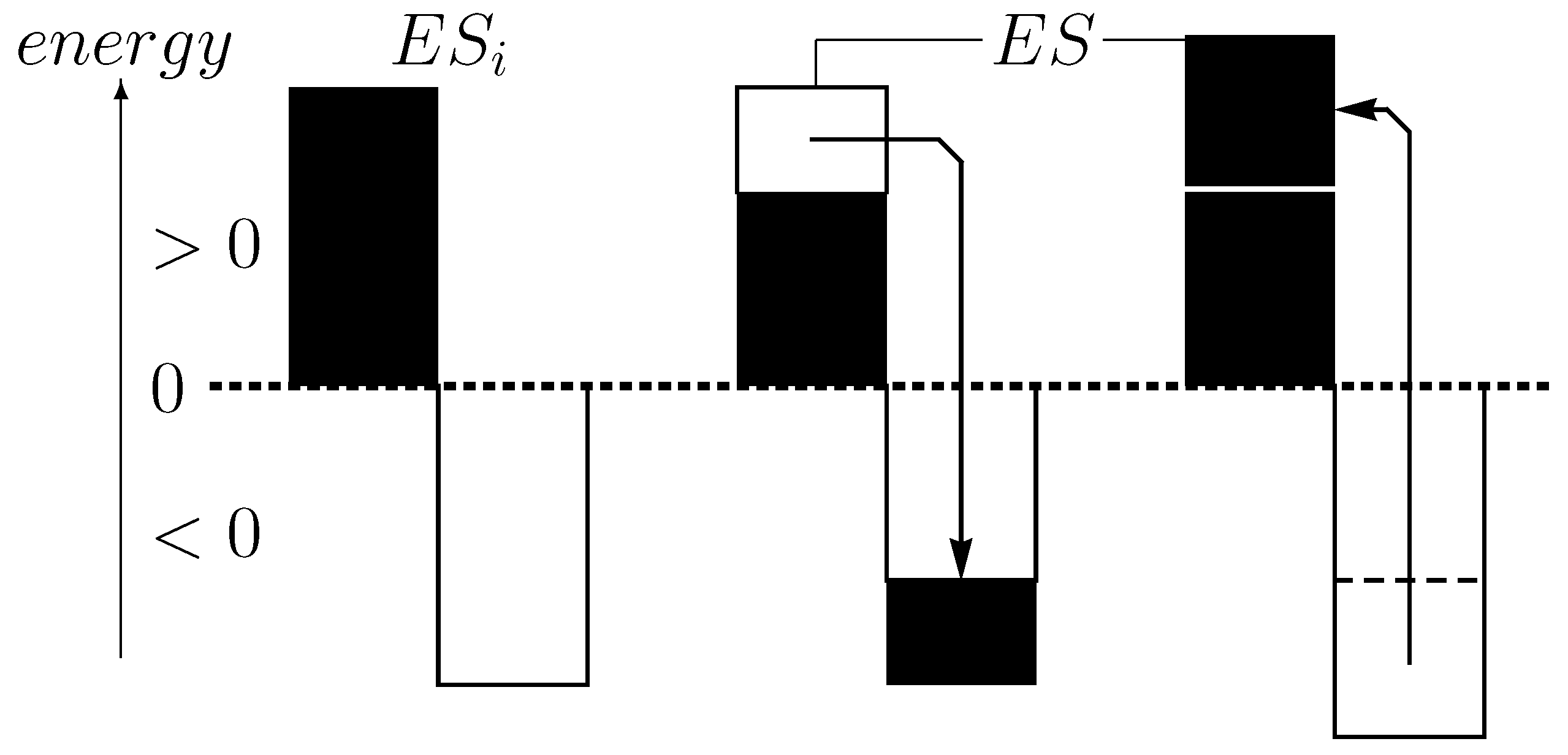
Figure 2.
Probability , obtained from numerical solutions of Eq. (17). The dashed vertical line is at size of the space quanta. Further details are provided in the main body.
Figure 2.
Probability , obtained from numerical solutions of Eq. (17). The dashed vertical line is at size of the space quanta. Further details are provided in the main body.
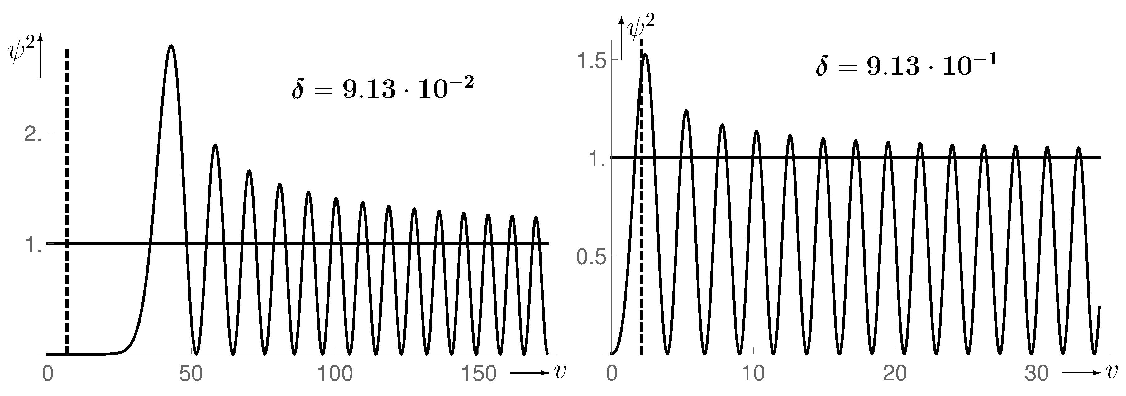
Figure 3.
Probability , obtained from the numerical solution of Eq. (20) for . The right picture shows the surroundings of the first maximum broadened in the v direction.
Figure 3.
Probability , obtained from the numerical solution of Eq. (20) for . The right picture shows the surroundings of the first maximum broadened in the v direction.
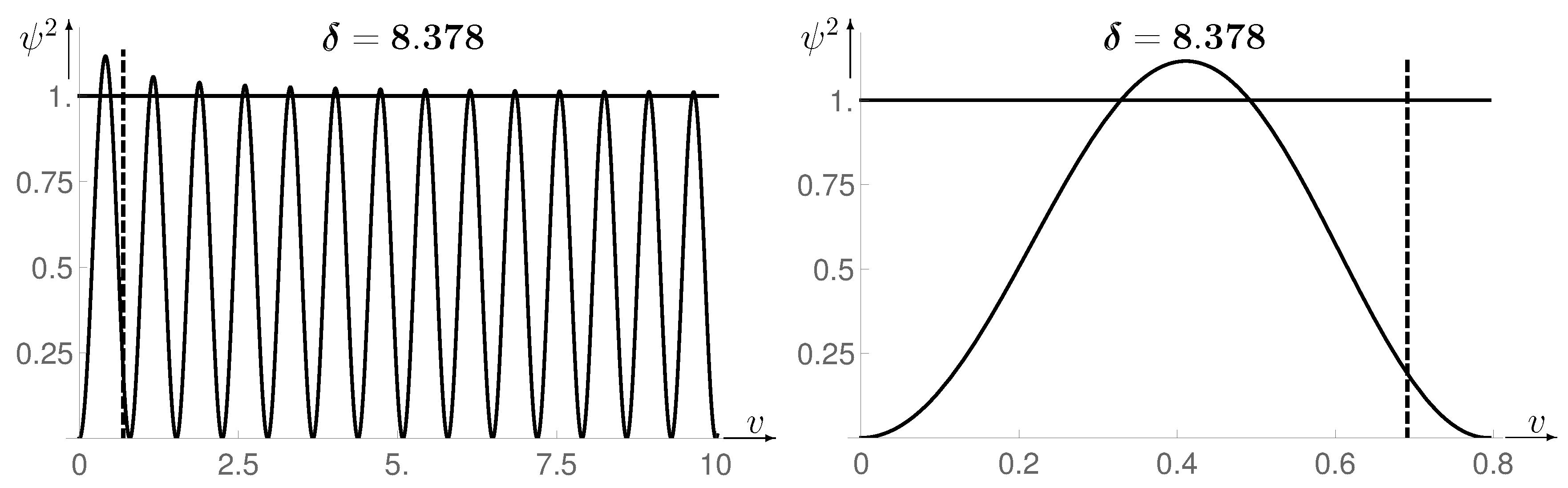
Figure 4.
Solutions of Eq (67) to the initial conditions (68) for small values of (). For and 15, the solution curves start shortly before so that their parabolic curvature at becomes visible. The amplitude of the curves increases for and decreases in turn for larger . Already for essentially the curve (81), calculated below for , is obtained.
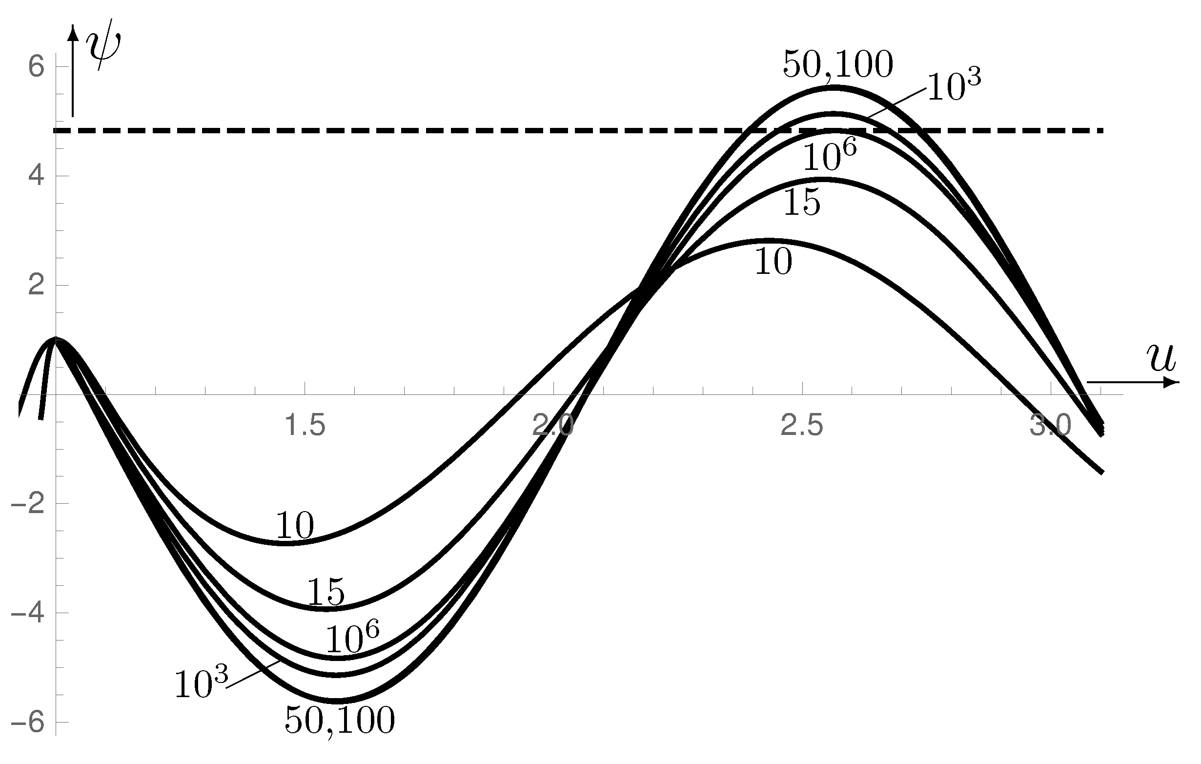

Table 1.
Comparison of solutions with different .
| LQG | ||||
|---|---|---|---|---|
| 1 | ||||
Table 2.
Characteristic values of .
| Formula | Value/( | ||
|---|---|---|---|
| 1 | |||
Table 3.
Characteristic values of .
| 0 | ∞ | ||||
|---|---|---|---|---|---|
| 1 | ∞ |
Table 4.
Mass of space quanta.
| time t | 0 | ||
|---|---|---|---|
Table 5.
Characteristic values of .
| time | 0 | |||
|---|---|---|---|---|
Disclaimer/Publisher’s Note: The statements, opinions and data contained in all publications are solely those of the individual author(s) and contributor(s) and not of MDPI and/or the editor(s). MDPI and/or the editor(s) disclaim responsibility for any injury to people or property resulting from any ideas, methods, instructions or products referred to in the content. |
© 2024 by the authors. Licensee MDPI, Basel, Switzerland. This article is an open access article distributed under the terms and conditions of the Creative Commons Attribution (CC BY) license (http://creativecommons.org/licenses/by/4.0/).
Copyright: This open access article is published under a Creative Commons CC BY 4.0 license, which permit the free download, distribution, and reuse, provided that the author and preprint are cited in any reuse.


