
Submitted:
28 February 2024
Posted:
28 February 2024
You are already at the latest version
Abstract
Chemical process control relies on a tightly controlled, narrow range of margins for critical variables, ensuring process stability and safeguarding equipment from potential accidents. The availability of historical process data is limited to a specific setpoint of operation. This challenge raises issues for process monitoring in predicting and adjusting to deviations outside of the range of operational parameters. Therefore, this paper proposes simulation-assisted deep transfer learning for predicting and optimizing the final purity and production capacity of the glycerin purification process. The proposed network is trained by the simulation domain to generate a base feature extractor, which is then fine-tuned using few-shot learning techniques on the target learner to extend the working domain of the model beyond the historical practice. The result shows that the proposed model improved prediction performance by 99% in predicting water content and 79.72% in glycerin prediction over the conventional deep learning model. Additionally, the implementation of the proposed model identified the production and product quality improvement for enhancing the glycerin purification process.
Keywords:
glycerin purification
; few-shot learning
; production optimization
; simulation-assisted.
1. Introduction
Biodiesel, a renewable energy source, is gaining prominence as the world seeks sustainable alternatives to fossil fuels. Its production, derived from natural sources such as vegetable oils, animal fats, and recycled greases, has grown significantly in recent years [1]. This increase is primarily driven by global commitments against climate change and the push towards greener energy sources. The production process of biodiesel involves transesterification, where fats and oils are converted into fatty acid methyl esters. An often-overlooked by-product of biodiesel production is glycerin. For every ten pounds of biodiesel produced, approximately one pound of glycerin is generated [2]. Despite being a by-product, glycerin holds immense value in various industries. However, the glycerin produced typically contains impurities and contaminants, necessitating purification to meet quality standards. This purification process, which removes unwanted substances such as water and fatty acids, faces challenges due to a limited operating domain and a narrow control range. These constraints hinder its ability to effectively and efficiently remove the wide array of impurities found in glycerin by-products from biodiesel production, posing a significant challenge in consistently producing high-quality glycerin [3].
Accurately predicting process efficiency is crucial, especially under operating conditions that extend beyond the standard monitoring range. This complexity raises challenges in determining controller actions to compensate for process disturbances while ensuring the desired product quality is maintained [4]. A prime example is observed in glycerin purification. Critical factors such as the composition of the feed stream, the water-to-glycerin ratio, the performance of the evaporation unit, and adjustments of manipulated variables in the distillation column must be meticulously managed. These adjustments are necessary not only to maintain the quality of refined glycerin but also to ensure that the controller actions are effective within the unit operation constraints.
Expert engineers frequently modify these conditions, relying on their specialized knowledge and on-site experimental data [5]. However, the limited scope of most operating variables can often hamper the efficiency of glycerin purification. The complexity of the process increases due to the multitude of variables influencing operating conditions, which can lead to process instability [6]. Consequently, this challenge has led researchers to turn their focus toward utilizing artificial intelligence (AI) and data-driven techniques [7]. These methods offer the ability to analyze large datasets, identify patterns, and make predictions or real-time decisions using the information provided [8]. Even if the prediction skill of the AI-based method is high, the result can be deviated by multiple characteristics of process operation [9].
In chemical process optimization, four commonly found challenges from the data characteristics are uncertainty, multi-rate information, cyclic operation, and limited data [10]. Researchers have proposed multiple innovative techniques to resolve these challenges. Regarding uncertainty, Panjapornpon et al. introduced a deep learning model constructed using compensation architecture for energy optimization addressing uncertainties in measurement [11]. Similarly, Wiebe, Cecilo, and Misener integrated data-driven stochastic degradation models with optimization strategies, using robust techniques to manage uncertainties in equipment degradation. Lastly, Moghadasi et al. proposed a gradient boosting machine with density-based spatial clustering of application with noise to optimize the steam consumption in the gas sweetening process [12]. These contributions show that the advancement of the data-driven method can be significantly useful in resolving the challenge facing industrial processes. However, a common thread among these techniques is their reliance on large datasets. The integration of data cleaning methods and network architecture modification can remove the contribution made by process disturbances, but it requires a lot of training information, as well as careful tuning of the network parameters, to ensure that the resulting model accurately reflects the underlying system dynamics without being overly influenced by noise or irrelevant data [13]. This approach typically involves iterative refinement of both the data preprocessing steps and the network architecture to strike a balance between model complexity and generalization ability [14].
When encountering complex scenarios such as the chemical industry, the framework of the AI-based model might change following the challenges that the research focuses [15]. Han et al. proposed a feed-forward neural network (FNN) with data envelopment analysis (DEA) for production optimization of ethylene production [16]. The integration of DEA with a deep learning model can help in optimization, but based on its architecture, the network might not effectively capture all nonlinear relationships. This can be resolved by using the recurrent neural network, such as long short-term memory (LSTM) [17]. The network has a recurrent interval state that helps in handling long-term dependency found in the data [5]. The performance of the LSTM network can be improved by the incorporation of an attention mechanism (AM). AM-LSTM is particularly useful in tasks where the sequence is long and not equally important along the sequence by allowing the network to weight diverse parts of input differently [18]. However, despite these advancements, AM-LSTM networks still face challenges in terms of adaptability and scalability, particularly when dealing with limited data scenarios, both in terms of quantity and domain-specific data. To resolve this issue, Han et al. proposed a hybrid approach using Monte Carlo (MC) simulation to expand the working domain of the LSTM network [19]. By simulating a wide range of possible scenarios, the MC-LSTM model can effectively deal with limited data situations. Since it provided an improvement, it is important to note that MC simulation is inherently probabilistic, relying solely on random sampling techniques. Integration of digital twin technology offers a more holistic and accurate simulation [20]. Digital twins create dynamic virtual representations of physical systems, allowing for more detailed and realistic scenario modeling while perfectly eliminating limited data problems [21].
Therefore, this study proposes the model developing framework using LSTM with simulation-assisted few-short learning (FSL-LSTM) for predicting and optimizing the glycerin product purity of the glycerin purification process and water removal of the evaporating unit under feed uncertainty and limited data. The model is trained to create a support feature extractor and weight initializer using a simulated support set, which is then used to fine-tune the prediction model in the limited data domain using a query set obtained from the large-scale glycerin purification unit. The main contribution of the proposed procedure is summarized as follows:
- Develop a glycerin purification process simulation model to determine optimal operating conditions and generate data for the support set.
- Formulate a robust predictive model based on deep learning constructed using LSTM structure fine-tuning based on few-shot learning techniques for tracking the refined glycerin production capacity and water content of refined glycerin under multiple operating conditions.
- Reveal the relationship between the input variables and the target variables of the prediction model to enhance the production capacity and water content using the proposed model.
The remainder of this work is divided into the following sections: Section 2 explains the concept of modeling procedure in developing FLS-LSTM, which includes few-shot learning, LSTM architecture, and Bayesian optimization. Section 3 presents the case study utilized in this study, incorporating system description and comparison between support and query data. Section 4 shows the performance of the proposed model in predicting glycerin production and water content, accuracy-iteration tradeoff, and production optimization results. Finally, conclusions are drawn in Section 5.
2. Materials and Methods
2.1. Simulation-assisted few-shot learning
Few-shot learning stands as a technique enabling models to understand or infer information from a very limited amount of data, which is the main focus of this study. Figure 1 depicts the schematic of a simulation-assisted few-shot learning system designed to enhance the learning process by integrating simulated support data. The system comprises several key components:
- Support and query data: The model operates on two datasets, including the support data (xs), which is excess data used to pre-train the model obtained by simulation, and the query data (xq), which refers to the limited data utilized to fine-tune and evaluate the ability of the model to generalize obtained by actual data from the large-scale glycerin purification process.
- Deep neural network: A deep neural network, in this case, LSTM (discussed in Section 2.2), functions as a feature extractor. It is optimized using the support data to derive representations that can be adapted to unseen query data or shared between domains.
- Normalization block: Within the neural network, a normalization procedure is applied to regulate the feature scaling. This can significantly help the model maintain and stabilize the training dynamics. Both input and output variables are rescaled into zero to one [0,1] using Equation (1).
- (1)
- Support initializer and extender predictor: The initializer is used to create the predictor initial weights (Ws) based on the support data, embedding the gained knowledge into the model. Subsequently, the extended predictor undergoes a few-shot learning phase using the limited query data to predict the final output (yq). In this step, partial layer freezing is applied to the initial weights to prevent overfitting and preserve previous knowledge gained from the support data while adapting to the specific query data. Only the modifying weights (Wq) are adjusted during fine-tuning using the loss gradient from query data, where the loss is a half-mean-squared error (HMSE) calculated by Equation (2). The local learning rate of initial weight is set to zero during the fine-tuning step.
where is the prediction value, is the target value, M is the total number of responses in , and N is the total number of observations in .
The proposed framework begins with using the information from the query set to set up the simulation boundary. This is followed by the development of the simulation-assisted using UniSim Design Suite to generate a support set (simulation data). The process continues with data normalization performed on both domains. Next, the model used the information from xs to train the support feature extractor and initializer, preparing the model with initial parameters that can be further refined. Bayesian optimization is applied in this step to find the best combination of hyperparameters such as hidden node, learning rate, and regularization factor.
Once the support data training is completed and the optimal hyperparameters for the support set are identified, the fine-tuning of the FSL-LSTM model using xq is performed. Again, the Bayesian optimization is applied to find the hyperparameters for the query set. Finally, the process concludes with the final FSL-LSTM model, which is then evaluated for its performance using metrics such as coefficient of determination (R2), mean squared error (MSE), and mean absolute error (MAE), calculated by Equations (3)–(5), respectively. These metrics provide a quantitative measure of how well the model is performing, indicating its accuracy and precision in predicting glycerin production and water content based on the limited query data. The overall framework for developing the FSL-LSTM framework is summarized in Figure 2.
In summary, each step in the framework of FSL-LSTM plays a vital role in ensuring that the model is not only pre-trained on a broad range of simulated data but also finely tuned to real-world scenarios. This modeling approach allows for a more robust and adaptable model capable of handling the complexities and limited data problems without raising concerns about domain differences.
2.2. LSTM network architecture
Handling complex relationships, such as the information from industrial processes, requires a network that can capture temporal dynamics and long-term dependency [22]. In recent years, LSTM has emerged as a fundamental component in the field of deep learning, especially for tasks that require processing sequential and time-series data. An LSTM network consists of a sequence of recurrent modules called LSTM cells. Every cell comes with gates, which are systems that control the flow of information inside the LSTM structure. These gates - the forget gate, input gate, and output gate - allow LSTMs to selectively remember and forget patterns over long sequences of data, as visualized in Figure 3. Inside the LSTM layer, the long-term memory is updated at the forget gated by using the cell state of the previous timestep using Equation (6).
Then, the input gate filters out unnecessary information, and only a significant part of the input will perform point-wise multiplication with the old state variable to create a cell candidate using Equations (7)–(9).
At the output gate, the updated cell state is used to determine the final values of the hidden state for the next layers using Equations (10) and (11).
A state is is contains a unit of LSTM at the time t, and it is controlled through the forget gate , input gate , candidate cell , and output gate ,is the vector of input variables at the time , and is the previous value of the hidden state.
2.3. Bayesian optimization for hyperparameter tuning
Bayesian optimization acts as a strategic tool in this process, seeking to fine-tune the hyperparameters by iteratively minimizing the objective function, which this study used validation MSE. Figure 4 illustrates the utilization of Bayesian optimization for tuning the hyperparameters in a glycerine purification process model. The process begins with the training model acting as an observer to evaluate the initial combination of hyperparameters for fitting the surrogate model (Gaussian process regression). The Expected Improvement (EI) acquisition function, calculated using Equation (12), then guides the selection of subsequent hyperparameters, aiming to maximize the expected improvement over the best current validation MSE. This is particularly useful in a few-shot learning scenario, where the model needs to generalize well from a limited amount of data. By carefully choosing where to sample next, EI helps to efficiently navigate the hyperparameter space specified in Table 1, reducing the number of iterations needed to find an optimal set of hyperparameters compared to optimization techniques such as grid-search. The process is performed iteratively until the specified iteration is reached (50 iterations), indicating that the model has potentially reached an optimum. The outcome of this process is a set of hyperparameters finely tuned to the few-shot learning task, which will be used as a final model for glycerine production and water content optimization.
where xbest as the location of the lowest posterior mean and (xbest) as the lowest value of the posterior mean.
3. Glycerin purification case study
3.1. Process description
Figure 5 illustrates the process flow diagram of the glycerin purification process under study. The process comprises three main units: neutralization, evaporation, and glycerine distillation. Initially, the crude glycerine feed, containing glycerin, water, fatty acids, and other impurities, is preheated in a heat exchanger. This pre-treatment step is crucial before sending the mixture to the neutralization unit. In the neutralization unit, a sodium hydroxide solution (at a ratio of 0.5 mol/mol and room temperature) is used to adjust the pH to a range of 7.0 to 9.0.
Since water content significantly affects the purity of glycerin during production, the neutralized mixture is then forwarded to the evaporation unit. Here, the mixture undergoes drying through a water evaporation process. Since water has a much lower boiling point than glycerin, this step effectively reduces the water content. The evaporator’s temperature must be carefully adjusted according to the feed compositions to achieve the desired water content, making evaporation a critical stage in the process. The target is to reduce the water content of the mixture to below 2% before proceeding to the next stage. Subsequently, the glycerin, now with reduced water content, is sent to a distillation column for further purification. The distillation process aims to achieve a glycerin purity of 98-99%. The column used for this purpose is a five-stage structurally packed column equipped with a two-stage rectifier and a total condenser. The primary role of each unit operation included in glycerin purification is given in Table 2.
In this study on glycerin purification, a series of input variables are identified to influence the output characteristics of the process. The glycerin and water content in the feed (X1 and X2) directly affect the quality of the output, as they determine the starting composition of the purification process. The mass flow rate of the feed (X3) and the distillation column feed rate (X5) are crucial for the throughput of the system, influencing both the production capacity (Y1) and the efficiency of water removal (Y2). The inlet temperature of the first heat exchanger (S-101) and the bottom temperature of the distillation column (X6) are key thermal inputs that drive the separation process, while the top and bottom pressures of the distillation column (X7 and X9) and the top temperature of the side stream (X10) are indicative of the energy and material balances within the system. The relationship between these inputs and the outputs—namely, the production capacity and the remaining water content in the purified glycerin—illustrates the complex interplay of thermal and material transfer within the purification process, where the list of input and output variables used in this study is given in Table 3.
3.2. Process simulation modeling
The simulation of the glycerin purification process was developed in the UniSim Design Suite Software using the nonrandom two-liquid thermodynamic and fluid model. To create comprehensive data sets, we utilized a co-simulation environment, integrating MATLAB with the UniSim Design Suite process simulator. This approach enabled us to simulate various process conditions, generating a substantial amount of data with 1000 sample points. Such a method ensures that our simulated data (support data) adequately represents the actual operational conditions (query data).
During the simulation, the crude glycerin feed compositions are varied. The adjustments included a range of 10%-20% water content, 80%-90% glycerin content, 1%-2% Matter Organic Non-Glycerol (MONG) content, and an acidity content between 0.06-0.1%. Additionally, the feed rate of the crude glycerin was altered between 3700 kg/h and 4500 kg/h. To replicate varying operational conditions, the top temperature of the distillation column, operating at atmospheric pressure, was modified between 120°C and 125°C. The simulation domain is summarized in Table 4.
Upon obtaining the 1000 data samples, the whole dataset is partitioned the data into distinct sets for training, validation, and testing. The distribution was as follows: 80% for training, 10% for validation, and the remaining 10% for the test set. The 80% in the training set is used to train the model, while the 10% in the validation set is used to evaluate the objective performance during hyperparameter optimization. Finally, the last 10% of the testing data set is applied to assess the performance of the final model after finishing training and hyperparameter tuning.
The histograms in Figure 6 display a comparison of simulated and actual operational data, providing insight into the potential to broaden the operating range of the process. Areas of strong overlap between support and query data indicate close alignment, suggesting the simulation reflects the validated operational range accurately, suggesting a high degree of correlation between the simulated environment and real-world operations. The proximity of the mean values across various parameters implies that the simulation can effectively mirror the actual process, making it a valuable tool for exploring extensions to the operating domain. Densities in the histograms suggest the frequency of certain conditions in both sets of data; where simulation data is denser at the extremes, it may indicate the potential for stable operation beyond current observed limits.
4. Result and Discussion
4.1. Water content and production capacity prediction result
The hyperparameters optimization applied to the FSL-LSTM using nine selected hyperparameters is shown in Figure 7. These optimized hyperparameters, chosen for observation, include the number of hidden layers, the number of hidden nodes, the initial learning rate, the L2 regularization, and the optimizer. As the number of iterations increases, the prediction error steadily decreases. This ongoing reduction indicates that the optimization process is effectively identifying better hyperparameter combinations. Notably, the FSL-LSTM model, after hyperparameter optimization, exhibits a significant decrease in minimum prediction error. This error drops from 0.1 to 0.02 as early as iteration 2 and remains stable until reaching its lowest point, 0.0149, at iteration 22. This minimum error value lies close to the estimated objective minimum line, further validating the effectiveness of the optimization approach. The best set of hyperparameters is located at 22 iterations. One essential point is that the optimal value for the learning rate is 0.0095. Furthermore, the remarkably low learning rate of 0.0095 highlights the importance of carefully adjusting the model’s pre-trained knowledge during fine-tuning. This minimal step size helps safeguard the valuable information encoded in the initial model, allowing it to serve as a strong foundation for learning task-specific details without causing a catastrophic forgetting of its general capabilities. This reflects that the pre-trained knowledge gained from the support data significantly helps the model during the training phase.
The comparative results of water content prediction focusing on the testing performance of the model are presented in Table 5. The accuracy performance of the testing model of water content. The FSL-LSTM model demonstrates a notable R2 value of 0.995, thereby evidencing its superior predictive accuracy compared to other traditional models: 0.793 for FNN, 0.204 for RNN, 0.149 for NARX, and 0.801 for LSTM. The result demonstrates that the FSL-LSTM provided a 24.3% improvement in R2 values in the case of LSTM with custom few-shot learning.
The effectiveness of the proposed model is further revealed by MAE values of 0.017, thereby surpassing the MAE values of FNN, RNN, NARX, and LSTM, which have MAE of 0.038, 0.099, 0.105, and 0.043, respectively. Compared to the case of traditional LSTM, the incorporation of few-shot learning fine-tuning using simulation-assisted reduced the error by 60% and up to 83% error reduction compared to other models in the study. Additionally, in the case of MSE values, the FSL-LSTM model records a minimal MSE value of 0.001, markedly lower than those recorded by FNN (0.009), RNN (0.067), NARX (0.075), and LSTM (0.009) with up to 98% error reduction.
Table 6 shows the comparative analysis for the glycerin production prediction using a testing dataset of glycerin production prediction. The FSL-LSTM model attains an R2 value of 0.895, outstripping FNN (0.541), RNN (0.309), NARX (0.397), and LSTM (0.498), which is 79.7% improvement in R2 values compared to the traditional LSTM. Additionally, the R2 performance improvement for the glycerine production prediction is higher than the improvement in water content.
In evaluating the MAE loss variable within this context, the FSL-LSTM model records an MAE of 0.050, a value that is demonstrably lower than those recorded by FNN (0.054), RNN (0.056), NARX (0.055), and LSTM (0.057). Despite the marginal disparities among the training models, the FSL-LSTM model exhibits a significantly reduced MAE value, exhibiting a 12.2% error reduction. Conclusively, the MSE evaluation of the model for production capacity further corroborates the FSL-LSTM superiority of the model. With an MSE value of 0.009, it presents a notable error reduction of 25% compared to the LSTM model.
Figure 8a shows the predicted production capacity of glycerin values from three different training models: the LSTM model, the FNN model, and the FSL-LSTM model, compared with the actual values (represented by a black line). Among these, the FSL-LSTM model (indicated by a red line) most accurately simulates changes in production capacity, closely aligning with the actual values. In contrast, the predictions from the LSTM model (shown in dark red) and the FNN model (depicted in orange) are less accurate, as evidenced by the divergence of their respective lines from the actual values, where the FSL-LSTM can track the abrupt process transition in changing production capacity.
Figure 8b focuses on the prediction performance of water content using FSL-LSTM. Here, the FSL-LSTM model is again notable for its accuracy, with its predictions (red line) closely mirroring the actual values. The LSTM model, while capable of capturing some characteristics of the actual data, falls short of the performance demonstrated by the FSL-LSTM model. Even in the water content prediction, where the noise in the process is relatively larger than the glycerin production prediction, the FSL-LSTM can accurately predict the water content under this scenario.
4.3. Accuracy-iteration in few-shot learning LSTM tradeoff
Figure 9 shows the result of decreasing and increasing the number of iterations in few-shot learning techniques. The model selection of FSL-LSTM is selected by the tradeoff between accuracy improvement among two outputs. The best number of iterations is obtained at two locations on this plot, 100 (maximum testing R2 of glycerin production is located) and 440 iterations (maximum testing R2 of water content is located)). At 100 iterations, the testing R2 values of Y1 and Y2 are 0.995 and 0.895, respectively, while the traditional LSTM performance without fine-tuning using few-shot learning is 0.495. This point provided a 99% improvement in water content prediction and a 79.72% improvement in glycerin production over the LSTM baseline. Furthermore, at 440 iterations, the R2 value of testing data for Y1 is 0.999, while Y2 is 0.547. At this point, the few-shot learning significantly improved the performance in water content prediction by up to 99.8%. However, the large improvement in Y2 results in an overfitting problem in Y1, where the testing performance drops substantially with only a 35% improvement. Thus, the justification of iteration count should be made with a primary focus on glycerin production prediction performance, and in this context, 100 iterations (1 datapoint per iteration) prove to be the optimal selection for few-shot learning with FSL-LSTM.
4.4. Production optimization result
After the FSL-LSTM is finally tested and its ability to track the water content and glycerin production, the operating condition adjustment is performed on the model to find the optimal condition for the glycerine purification process based on the prediction sensitivity. For example, Figure 10a shows the operational adjustment result for optimizing water content without changing glycerine production capacity. It can be seen that if the X1 and X3 are increased by 0.46 and 0.7 while X9 is reduced by 0.07, the water content in final glycerin product can reduced by 0.35.
In Figure 10b, there are optimization results for production maximization while the final water content remains constant. This can be done by reducing X1, X3, X6, X9, and X10 by 0.83, 0.69, 0.4, 0.23, and 0.09, respectively, and increasing X5 by 3. The production of glycerin will be improved by 0.34. Overall, these results illustrate the effectiveness of the FSL-LSTM model in guiding targeted operational adjustments for the glycerin purification process under limited operating data and working domain.
5. Conclusions
This study focuses on predicting and optimizing water removal in product and glycerin production capacity, under conditions of feed uncertainty and limited data. Utilizing the FSL-LSTM training model, coupled with Bayesian optimization for hyperparameter optimization, significant advancements are achieved over existing monitoring techniques. The model was trained using support data to create base learner, which are then applied the industrial data where the data is limited. This approach holds potential for application in other similar processes. The key contributions of this study include:
- (1)
- By utilization of digital-assisted few-shot learing approach, the proposed model achieved 0.895 and 0.955 in prediction R2 of glycerin production and water content, respectively. The incorpolated few-shot learning provides a 99% improvement in water content prediction and a 79.72% improvement in glycerin production over the LSTM baseline.
- (2)
- A simulation model for the glycerin purification process, capable of generating data for model use and determining optimal operating conditions. Though the Bayesian optimization, the updates with a low learning rate are more cautious, leading to a smoother convergence towards the optimal parameters and true function of output variables. This can be crucial for avoiding unstable training and achieving better generalization.
Author Contributions
T.J.: Methodology, software, validation, formal analysis, resources, data curation, writing—original draft preparation; C.P.: Conceptualization, validation, investigation, formal analysis, resources, visualization,, writing—original draft preparation, writing—review and editing, supervision, project administration, funding acquisition; S.B.: Validation, investigation, visualization, writing—review and editing; M.A.H.: Supervision, writing—review and editing. All authors have read and agreed to the published version of the manuscript.
Funding
This research is funded by Kasetsart University through the Graduate School Fellowship Program.
Data Availability Statement
Not applicable.
Acknowledgments
This research is funded by Kasetsart University through the Graduate School Fellowship Program. The author would like to acknowledge the support of the Faculty of Engineering, Kasetsart University, Center for Advanced Studies in Industrial Technology, and the Center of Excellence on Petrochemical and Materials Technology. Support from these sources is gratefully acknowledged.
Conflicts of Interest
The authors declare no conflict of interest.
References
- Moklis, M.H.; Cheng, S.; Cross, J.S. Current and Future Trends for Crude Glycerol Upgrading to High Value-Added Products. Sustainability 2023, 15, 2979. [CrossRef]
- Huang, H.; Jin, Q. Industrial Waste Valorization. In Green Energy to Sustainability; 2020; pp. 515–537 ISBN 978-1-119-15205-7.
- Sidhu et al. - 2018 - Glycerine Emulsions of Diesel-Biodiesel Blends and.Pdf.
- Sallevelt, J.L.H.P.; Pozarlik, A.K.; Brem, G. Characterization of Viscous Biofuel Sprays Using Digital Imaging in the near Field Region. Applied Energy 2015, 147, 161–175. [CrossRef]
- Panjapornpon, C.; Chinchalongporn, P.; Bardeeniz, S.; Makkayatorn, R.; Wongpunnawat, W. Reinforcement Learning Control with Deep Deterministic Policy Gradient Algorithm for Multivariable pH Process. Processes 2022, 10, 2514. [CrossRef]
- Liu, J.; Hou, G.-Y.; Shao, W.; Chen, J. A Supervised Functional Bayesian Inference Model with Transfer-Learning for Performance Enhancement of Monitoring Target Batches with Limited Data. Process Safety and Environmental Protection 2023, 170, 670–684. [CrossRef]
- Jan, Z.; Ahamed, F.; Mayer, W.; Patel, N.; Grossmann, G.; Stumptner, M.; Kuusk, A. Artificial Intelligence for Industry 4.0: Systematic Review of Applications, Challenges, and Opportunities. Expert Systems with Applications 2023, 216, 119456. [CrossRef]
- Quah, T.; Machalek, D.; Powell, K.M. Comparing Reinforcement Learning Methods for Real-Time Optimization of a Chemical Process. Processes 2020, 8, 1497. [CrossRef]
- Park, Y.-J.; Fan, S.-K.S.; Hsu, C.-Y. A Review on Fault Detection and Process Diagnostics in Industrial Processes. Processes 2020, 8, 1123. [CrossRef]
- Thebelt, A.; Wiebe, J.; Kronqvist, J.; Tsay, C.; Misener, R. Maximizing Information from Chemical Engineering Data Sets: Applications to Machine Learning. Chemical Engineering Science 2022, 252, 117469. [CrossRef]
- Panjapornpon, C.; Bardeeniz, S.; Hussain, M.A. Improving Energy Efficiency Prediction under Aberrant Measurement Using Deep Compensation Networks: A Case Study of Petrochemical Process. Energy 2023, 263, 125837. [CrossRef]
- Moghadasi, M.; Ozgoli, H.A.; Farhani, F. Steam Consumption Prediction of a Gas Sweetening Process with Methyldiethanolamine Solvent Using Machine Learning Approaches. International Journal of Energy Research 2021, 45, 879–893. [CrossRef]
- Panjapornpon, C.; Bardeeniz, S.; Hussain, M.A.; Vongvirat, K.; Chuay-ock, C. Energy Efficiency and Savings Analysis with Multirate Sampling for Petrochemical Process Using Convolutional Neural Network-Based Transfer Learning. Energy and AI 2023, 14, 100258. [CrossRef]
- Wiercioch, M.; Kirchmair, J. Dealing with a Data-Limited Regime: Combining Transfer Learning and Transformer Attention Mechanism to Increase Aqueous Solubility Prediction Performance. Artificial Intelligence in the Life Sciences 2021, 1, 100021. [CrossRef]
- Aghbashlo, M.; Peng, W.; Tabatabaei, M.; Kalogirou, S.A.; Soltanian, S.; Hosseinzadeh-Bandbafha, H.; Mahian, O.; Lam, S.S. Machine Learning Technology in Biodiesel Research: A Review. Progress in Energy and Combustion Science 2021, 85, 100904. [CrossRef]
- Han, Y.-M.; Geng, Z.-Q.; Zhu, Q.-X. Energy Optimization and Prediction of Complex Petrochemical Industries Using an Improved Artificial Neural Network Approach Integrating Data Envelopment Analysis. Energy Conversion and Management 2016, 124, 73–83. [CrossRef]
- Hochreiter, S.; Schmidhuber, J. Long Short-Term Memory. Neural Computation 1997, 9, 1735–1780. [CrossRef]
- Han, Y.; Fan, C.; Xu, M.; Geng, Z.; Zhong, Y. Production Capacity Analysis and Energy Saving of Complex Chemical Processes Using LSTM Based on Attention Mechanism. Applied Thermal Engineering 2019, 160, 114072. [CrossRef]
- Han, Y.; Du, Z.; Geng, Z.; Fan, J.; Wang, Y. Novel Long Short-Term Memory Neural Network Considering Virtual Data Generation for Production Prediction and Energy Structure Optimization of Ethylene Production Processes. Chemical Engineering Science 2023, 267, 118372. [CrossRef]
- Chen, K.; Zhu, X.; Anduv, B.; Jin, X.; Du, Z. Digital Twins Model and Its Updating Method for Heating, Ventilation and Air Conditioning System Using Broad Learning System Algorithm. Energy 2022, 251, 124040. [CrossRef]
- Bardeeniz, S.; Panjapornpon, C.; Fongsamut, C.; Ngaotrakanwiat, P.; Azlan Hussain, M. Digital Twin-Aided Transfer Learning for Energy Efficiency Optimization of Thermal Spray Dryers: Leveraging Shared Drying Characteristics across Chemicals with Limited Data. Applied Thermal Engineering 2024, 122431. [CrossRef]
- Agarwal, P.; Gonzalez, J.I.M.; Elkamel, A.; Budman, H. Hierarchical Deep LSTM for Fault Detection and Diagnosis for a Chemical Process. Processes 2022, 10, 2557. [CrossRef]
Figure 1.
The network training procedure of FSL-LSTM.
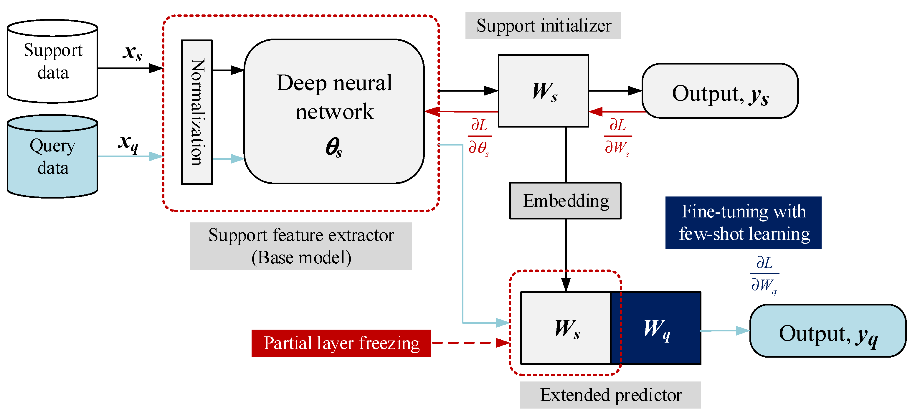
Figure 2.
The overall data-processing framework for model development.
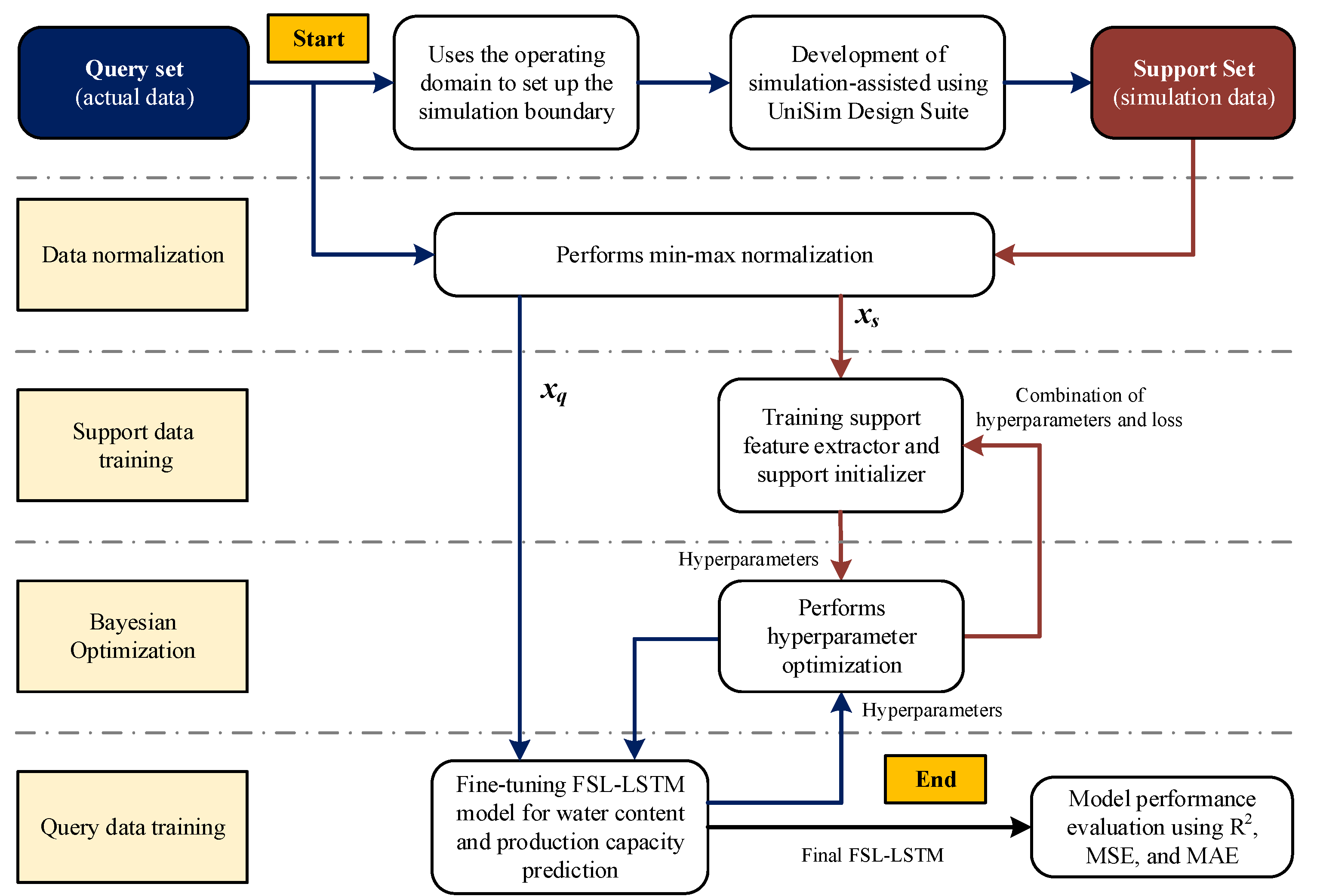
Figure 3.
The architecture and gating mechanism of the LSTM network.
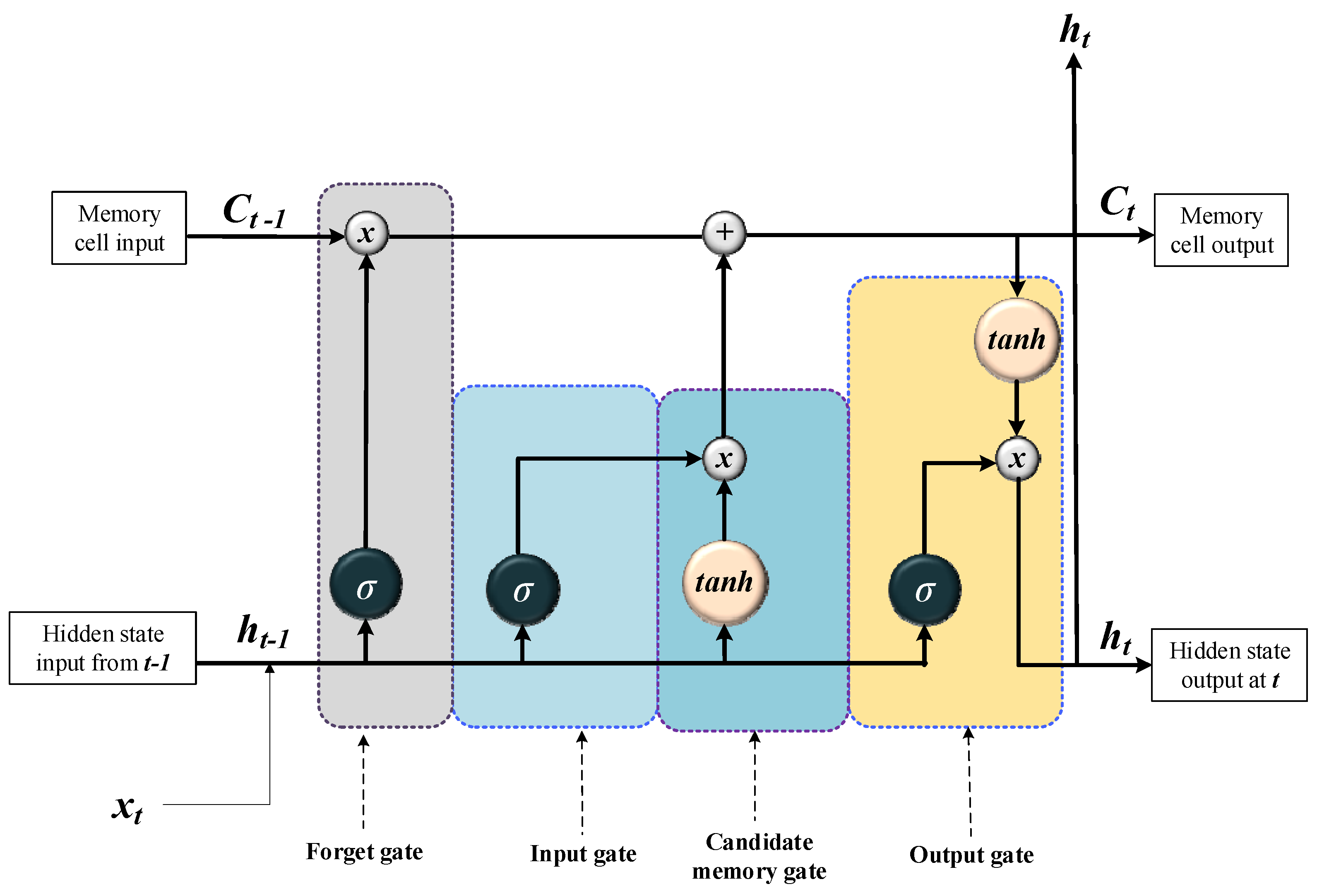
Figure 4.
Framework for hyperparameter tuning using Bayesian optimization.
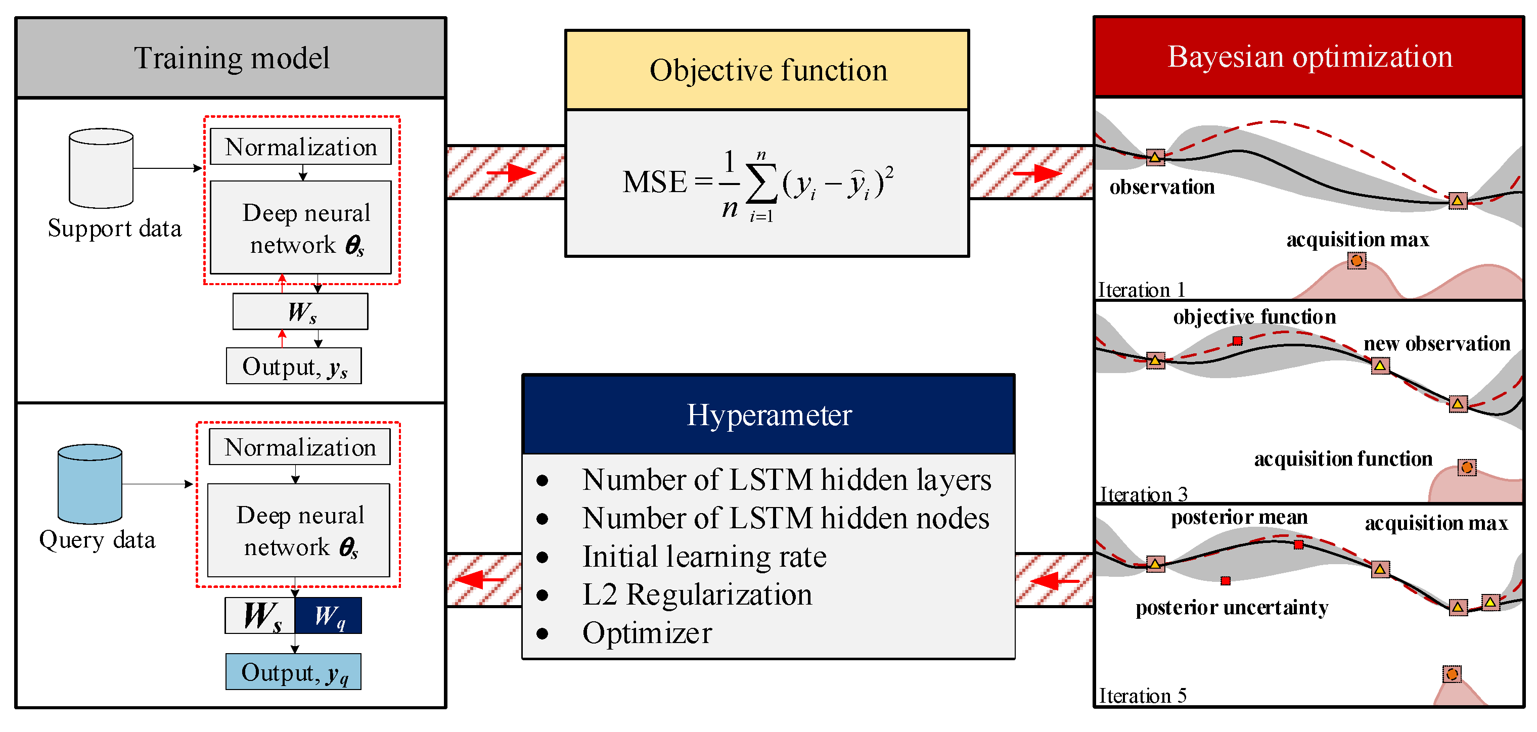
Figure 5.
Process flow diagram of the glycerin purification process.
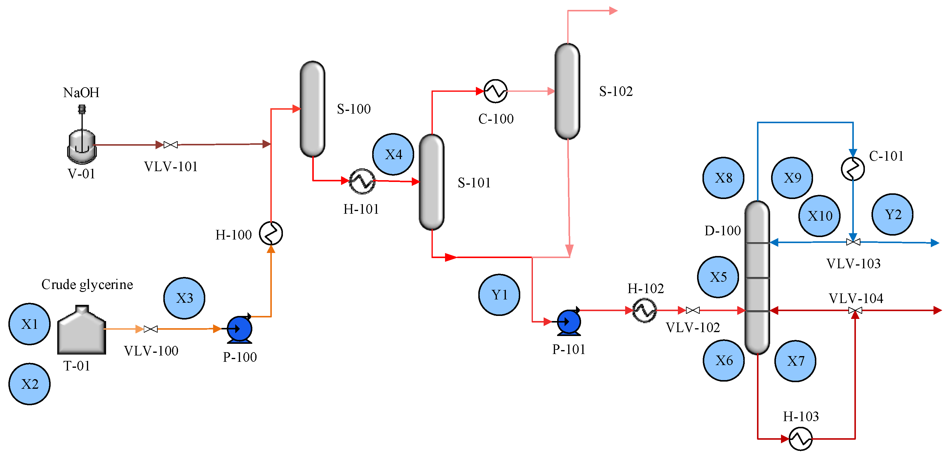
Figure 6.
The domain comparison between support data (simulation)and query data (actual).
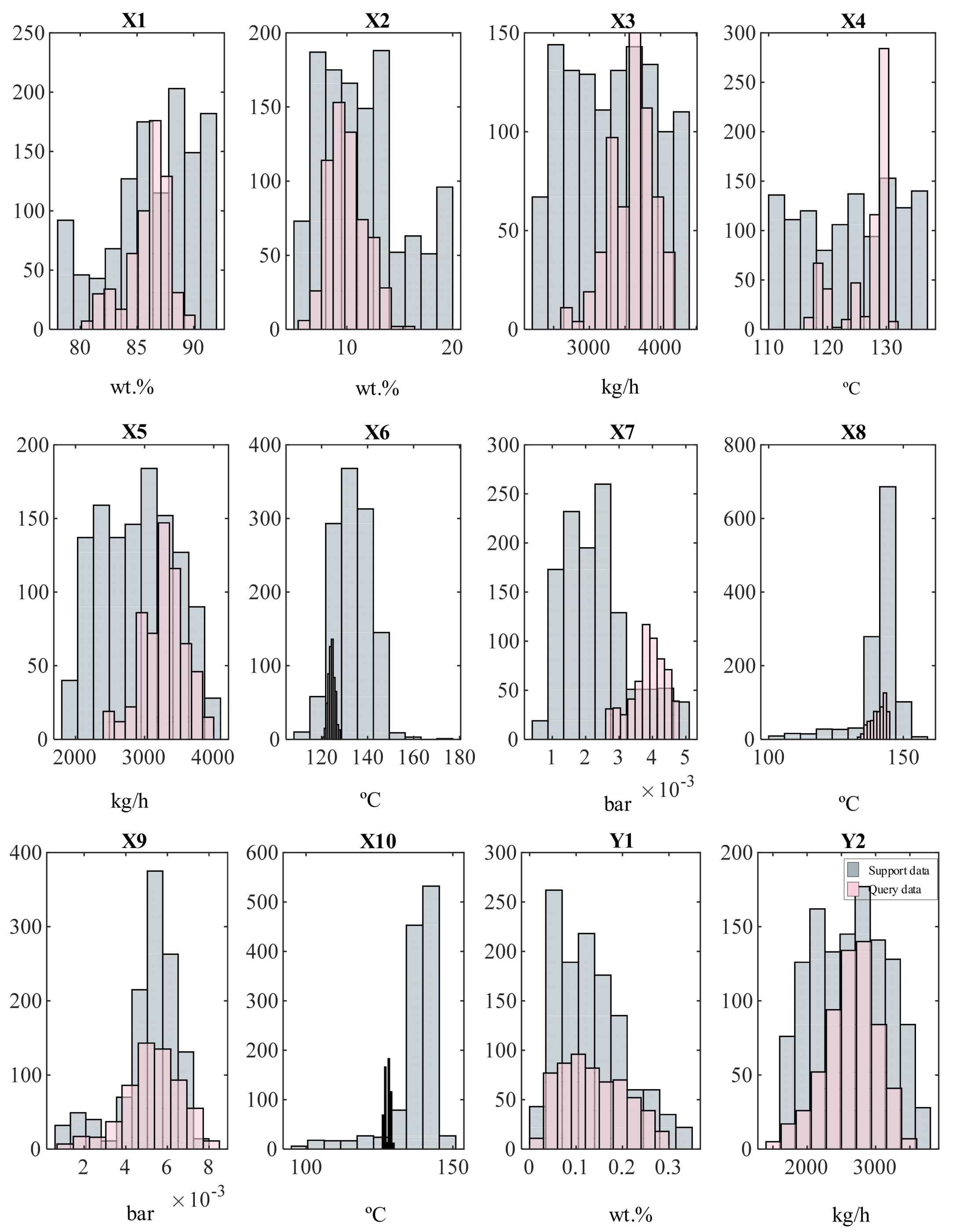
Figure 7.
The hyperparameter tuning result using Bayesian optimization.
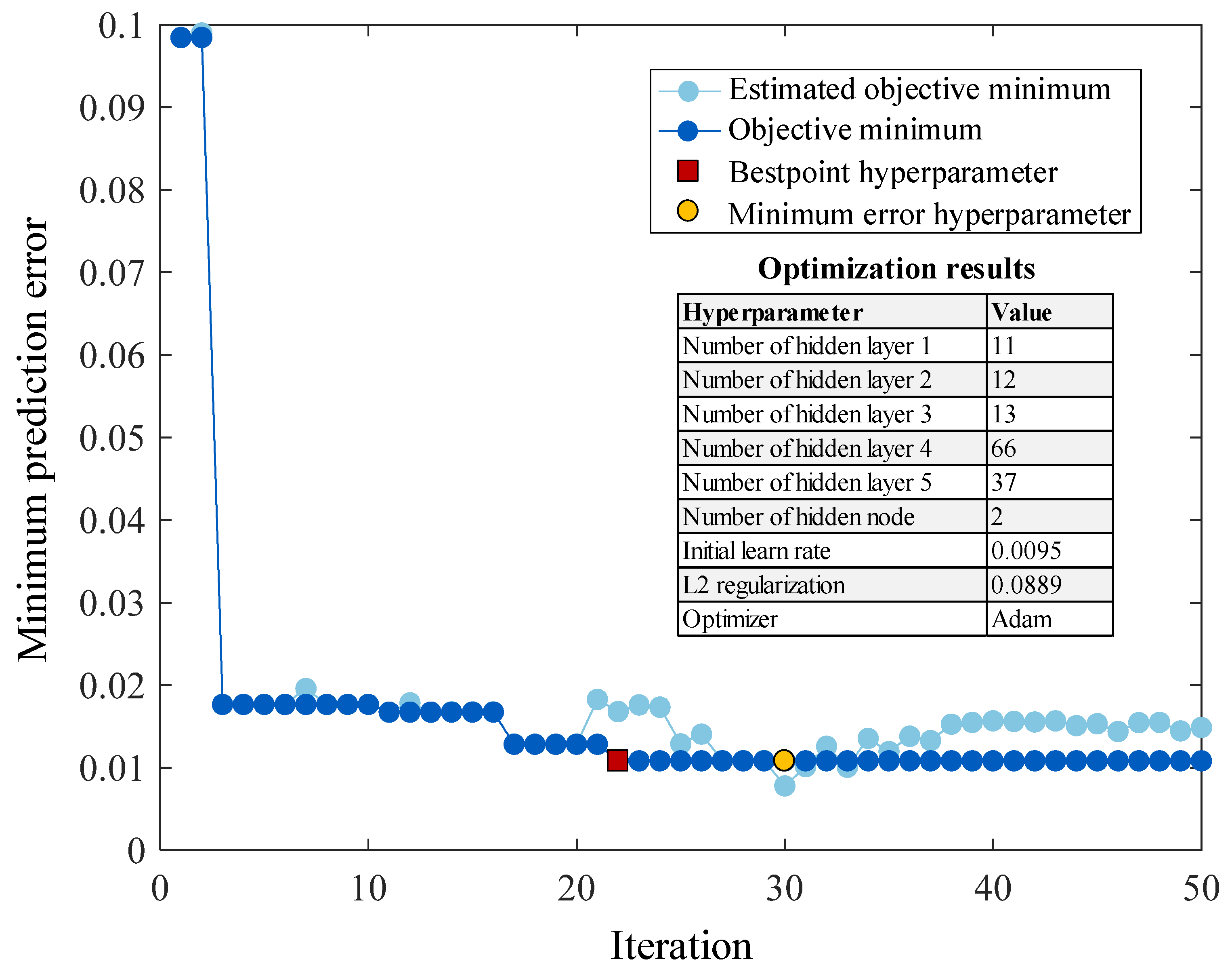
Figure 8.
Prediction performance for (a) production capacity; (b) water content.

Figure 9.
The tradeoff between accuracy improvement and the number of iterations used in few-shot learning.
Figure 9.
The tradeoff between accuracy improvement and the number of iterations used in few-shot learning.
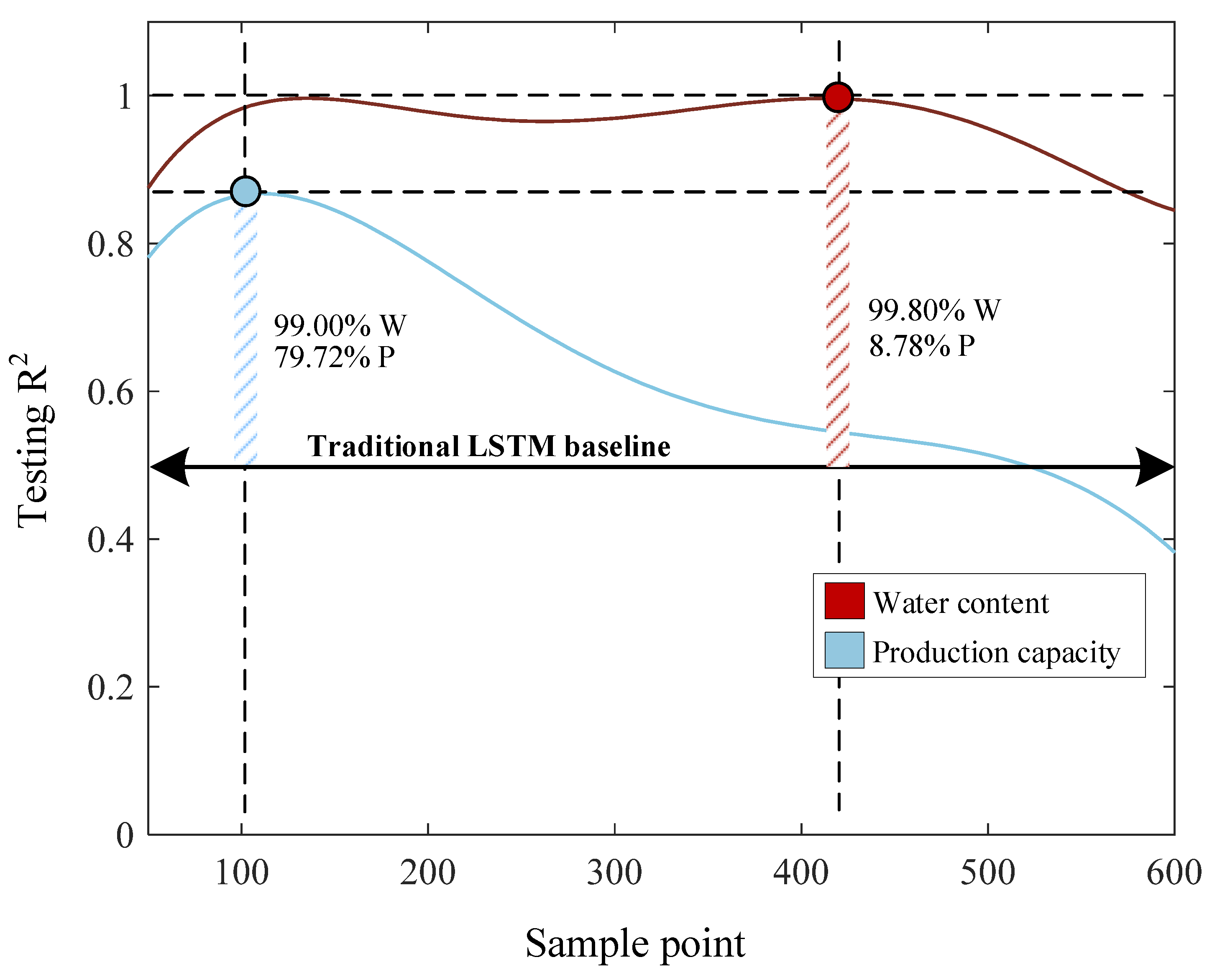
Figure 10.
FSL-LSTM guided optimization result for (a) water content and (b) glycerin production.
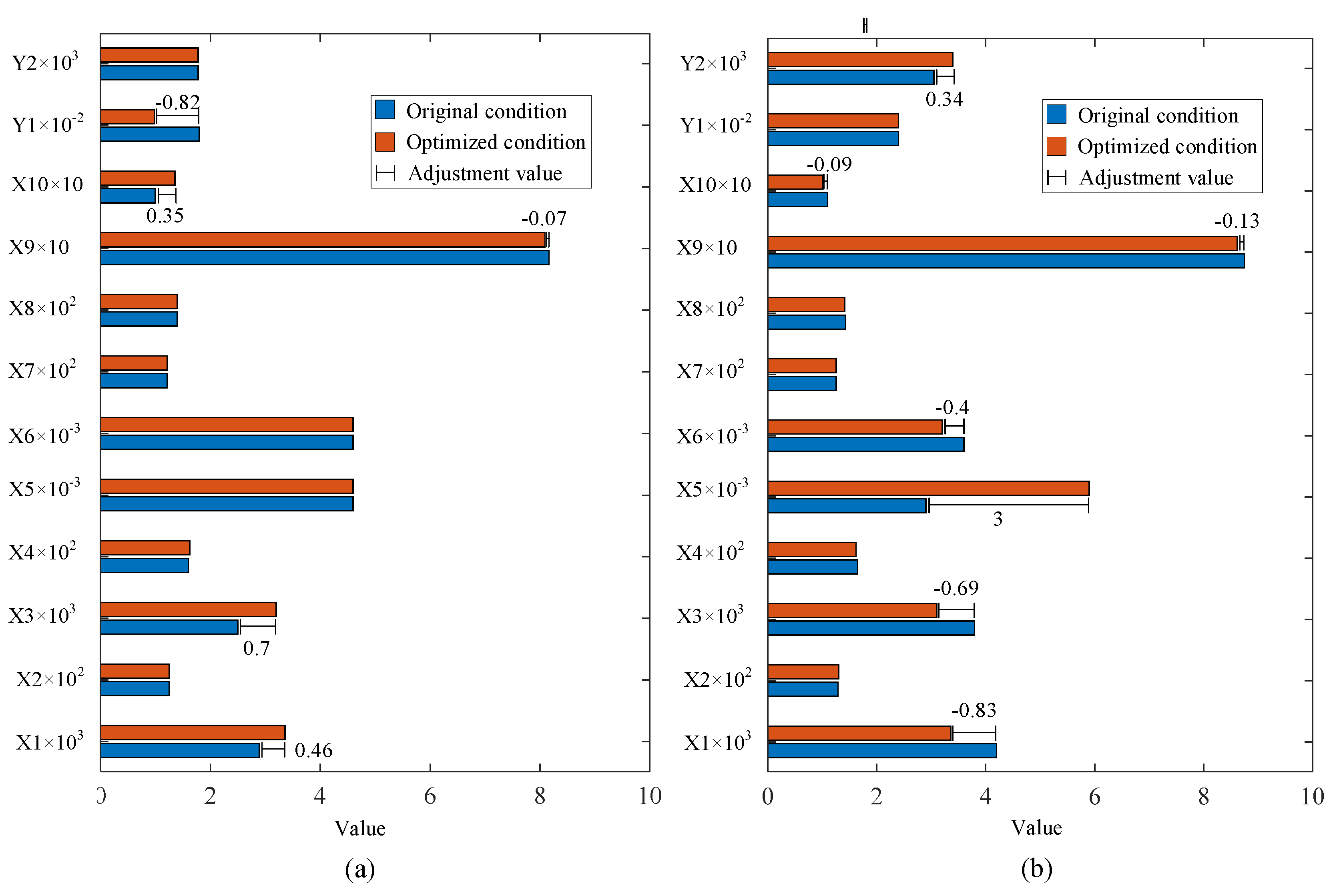

Table 1.
The search domain for hyperparameter tuning by Bayesian optimization.
| Hyperparameters | Value |
|---|---|
| Number of FNN hidden layers | [1– 100] |
| Number of LSTM hidden node | [1-5] |
| Number of LSTM hidden layersNumber of LSTM hidden node | [1– 100][1-5] |
| Number of NARX hidden layers | [1– 100] |
| Delay of NARX network | [1-5] |
| Number of RNN hidden layers | [1– 100] |
| Delay of RNN network | [1-5] |
| Initial learning rate | [1e-001 – 1e-005] |
| L2 Regularization | [1e-001 – 1e-004] |
| Max training iteration | 500 |
| Optimizer | [Adam, RMSProp, SDG] |
Table 2.
Role of each simulation unit operation in the glycerin purification process.
| Operation | Equipment | Unit | Duty |
|---|---|---|---|
| Neuralization process | Gibbs reactor | S-100 | A vessel that occurs in a transesterification reaction to obtain an outlet glycerin stream. |
| Evaporate process | Heater | H-101 | Heat mixed glycerin stream to 120 °C |
| Evaporator 1 | S-101 | Evaporator vapor stream and liquid glycerin stream | |
| Cooling | C-100 | Condense glycerin in the vapor stream | |
| Evaporator 2 | S-102 | Evaporate condenses glycerin and vapor of impurity | |
| Pump | P-101 | Boost pressure | |
| Purification process | Distillation column | D-100 | Purified glycerin to the desired purity |
| Condenser | C-101 | Condense an alloy glycerin to distillate | |
| Reboiler | H-103 | Heat glycerin returns to distillation and to the bottom product |
Table 3.
List of input and output variables used in this study.
| No. | Variable name | No. | Variable name |
| X1 | Glycerin content in feed, wt.% | X7 | D-100 bottom pressure, bar |
| X2 | Water content in a feed, wt.% | X8 | D-100 top temperature, oC |
| X3 | Feed mass flow rate, kg/h | X9 | D-100 top pressure, bar |
| X4 | S-101 inlet temperature, oC | X10 | Top temperature of side steam D-100, oC |
| X5 | Distillation column feed rate, kg/h | Y1 | Production capacity, kg/h |
| X6 | D-100 bottom temperature, oC | Y2 | Remaining water at evaporator outlet, wt.% |
Table 4.
The parameter range on the glycerin purification process.
| Name variable | Units | Setpoint | Range |
|---|---|---|---|
| Feed crude glycerin | |||
| Feed mass flow rate | kg/h | 3000 | [2500-400] |
| Component | |||
| Glycerin | wt.% | 88 | [80-90] |
| Water | wt.% | 10 | [10-20] |
| Evaporator | |||
| Inlet temperature | oC | 120 | [120-134] |
| Distillation column | |||
| Feedrate | kg/h | 2700 | [2300-3000] |
| Top temperature | oC | 125 | [125-130] |
| Top pressure | bar | 0.0025 | [0.001-0.005] |
| Bottom temperature | oC | 160 | [155-165] |
| Bottom temperature | bar | 0.0045 | [0.002-0.007] |
| Return top temperature | oC | 134 | [130-137] |
Table 5.
The performance evaluation result on water content prediction using a testing set.
| Method | MSE | MAE | R2 |
|---|---|---|---|
| FNN | 0.009 | 0.038 | 0.793 |
| RNN | 0.067 | 0.099 | 0.204 |
| NARX | 0.075 | 0.105 | 0.149 |
| LSTM | 0.009 | 0.043 | 0.801 |
| FSL-LSTM | 0.001 | 0.017 | 0.995 |
Table 6.
The performance evaluation result on glycerin production prediction using a testing set.
| Method | MSE | MAE | R2 |
|---|---|---|---|
| FNN | 0.011 | 0.054 | 0.541 |
| RNN | 0.028 | 0.056 | 0.309 |
| NARX | 0.036 | 0.055 | 0.397 |
| LSTM | 0.012 | 0.057 | 0.498 |
| FSL-LSTM | 0.009 | 0.050 | 0.895 |
Disclaimer/Publisher’s Note: The statements, opinions and data contained in all publications are solely those of the individual author(s) and contributor(s) and not of MDPI and/or the editor(s). MDPI and/or the editor(s) disclaim responsibility for any injury to people or property resulting from any ideas, methods, instructions or products referred to in the content. |
© 2024 by the authors. Licensee MDPI, Basel, Switzerland. This article is an open access article distributed under the terms and conditions of the Creative Commons Attribution (CC BY) license (http://creativecommons.org/licenses/by/4.0/).
Copyright: This open access article is published under a Creative Commons CC BY 4.0 license, which permit the free download, distribution, and reuse, provided that the author and preprint are cited in any reuse.


