
Submitted:
05 August 2025
Posted:
06 August 2025
You are already at the latest version
Abstract
The rise of Industry 4.0 has made robust forecasting and process control central to achieving sustainable smart manufacturing. While deep learning improves prediction accuracy, most models lack uncertainty quantification and process control—both critical for minimizing waste and optimizing energy use. Generative models are promising but underused in real-world manufacturing due to data and integration challenges. To address this, we propose a unified two-stage deep learning framework for real-time simulation and adaptive process control in dynamic manufacturing environments. The first stage leverages DeepAR and Monte Carlo Dropout to produce both accurate point predictions and calibrated uncertainty intervals. The second stage introduces a novel LSTM-based Conditional Variational Autoencoder (LSTM-CVAE) that reconstructs temporally coherent multivariate input sequences conditioned on target specifications. Then a two-stage filtering mechanism ensures the plausibility of generated inputs and their predictive alignment with operational goals. Experiments on two real-time industrial datasets (sugar and bioprocessing) and a public benchmark demonstrate average improvements of up to 35.7%, 21.0%, 24.6% in Balanced MAE, and 21.3%, 9.8%, 25.2% in Comprehensive Uncertainty Score metrics. The framework remains robust under batch-wise shuffling, supporting real-world deployment. Overall, it enables interpretable, forecast-aware, target-driven process control that improves resource efficiency and product cost—advancing sustainable manufacturing.
Keywords:
Industry 4.0
; artificial intelligence
; uncertainty-aware forecasting
; generative modeling
; process control
; sustainable manufacturing
1. Introduction
The emergence of Industry 4.0 has driven the convergence of cyber-physical systems, the Internet of Things (IoT), cloud computing, and big data analytics in modern manufacturing environments, generating large volumes of multivariate time-series data from machines, processes, and operating conditions [1,2,3]. These digital transformations enable advanced data-driven decision-making, which is critical not only for improving operational efficiency and product quality, but also for promoting sustainability through reduced energy consumption, waste minimization, and predictive maintenance. Leveraging recent advances in machine learning (ML) and deep learning (DL), Industrial AI has emerged as a powerful paradigm to extract actionable insights from complex manufacturing data [4,5]. However, realizing the full potential of these technologies remains challenging due to the high dimensionality, heterogeneity, and noise inherent in real-world industrial datasets [6]. Addressing these challenges is essential to support sustainable and intelligent manufacturing operations.
1.1. Background
Industry 4.0 builds upon the digital automation of Industry 3.0 by introducing interconnected, intelligent machines capable of decentralized decision-making and adaptive control without direct human input [7]. This transformation is largely driven by the integration of ML and DL algorithms, which enable manufacturing systems to perform complex tasks and adapt to dynamic conditions based on data-driven insights rather than predefined rules [8]. These algorithms are typically categorized into supervised and unsupervised learning, depending on the nature of data labeling and learning objectives [9].
In smart manufacturing, ML and DL enable four levels of analytics: descriptive, diagnostic, predictive, and prescriptive [10]. Descriptive analytics provides a summary of historical operations—e.g., Iftikhar et al. [11] visualized sensor data to identify downtime patterns. Diagnostic analytics uncovers root causes of issues, as in the CNN-LSTM-GRU model used by Han et al. [12] for detecting faults in rotating equipment. Predictive analytics forecasts future events such as Remaining Useful Life (RUL), supporting proactive maintenance strategies as demonstrated by Kang et al. [13]. Finally, prescriptive analytics recommends optimal actions to enhance outcomes, such as the reinforcement learning framework developed by Lepenioti et al. [14] for sustainable process control in steel manufacturing. Together, these analytics form the backbone of intelligent decision-making in operations, contributing not only to improved efficiency and quality but also to enhanced sustainability by reducing waste, energy consumption, and unplanned downtime.
Beyond traditional manufacturing, ML and DL have found broad applications in enabling sustainable practices across diverse industries. These include real-time decision-making in embedded AI systems [15], energy-aware adaptive factory systems [16], health and performance monitoring for human-centric manufacturing [17], optimization of energy systems for environmental sustainability [18], autonomous transportation for emission reduction [19], and AI-powered precision agriculture for maximizing yield with minimal environmental impact [20]. These examples demonstrate the critical role of AI technologies in advancing both operational excellence and sustainability across domains.
1.2. Issue
Despite the transformative potential of ML and DL in industrial settings, several barriers continue to limit their practical deployment in smart manufacturing environments. One major challenge is the organizational knowledge gap in AI: many manufacturing firms lack a clear understanding of how to collect, preprocess, and leverage high-value operational data, which undermines model reliability, scalability, and trustworthiness [21]. This gap poses a significant risk to achieving the goals of sustainable and resilient operations.
Traditional ML models often struggle to manage the dynamic and time-dependent nature of industrial processes [22,23]. A key concern is concept drift, where underlying data distributions evolve over time, leading to severe degradation in model performance once deployed. This disconnect between training and real-world conditions hinders effective decision-making and can result in wasteful or even unsafe operational outcomes [24]. Two primary obstacles restrict the effectiveness of ML/DL in production environments:
- Insufficient data volume and quality: Industrial data is often sparse, noisy, and inconsistent due to sensor malfunctions, heterogeneous sources, or environmental variability. Preprocessing is time-intensive, and accurate labeling is resource-intensive and error-prone [25,26]. These issues reduce model performance and impede sustainable insights generation.
- Limited model adaptability and transferability: ML/DL models trained for specific machines, production lines, or factories often fail to generalize across different settings. Overfitted models lack robustness, while overly generic models miss critical domain-specific dynamics. Furthermore, many existing forecasting models provide only point estimates, lacking mechanisms to quantify uncertainty—an essential capability in sustainability-critical or safety-sensitive applications [27].
Addressing these issues is critical to building intelligent, adaptive, and trustworthy decision-support systems that can contribute to sustainable manufacturing outcomes. To that end, robust frameworks are needed that:
- Adapt to concept drift while preserving model performance over time,
- Quantify predictive uncertainty to improve confidence in decisions and support risk-aware operations,
- Generalize effectively across diverse processes, equipment, and industrial contexts.
1.3. Our Idea
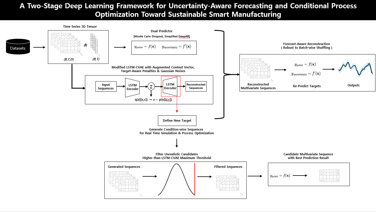
This study proposes a two-stage deep learning framework designed to enhance decision-making reliability and adaptability in dynamic manufacturing systems, with an emphasis on sustainable and resilient operations. The architecture integrates both predictive and generative components, structured as follows:
- Uncertainty-aware forecasting module: Provides calibrated point predictions along with probabilistic confidence intervals, enabling risk-aware decision support under dynamic conditions.
- Conditional generative module (LSTM-CVAE): Reconstructs realistic multivariate input trajectories conditioned on desired outcomes or target distributions, allowing controllable scenario generation.
Together, these modules empower manufacturing systems to capture temporal dynamics while simulating feasible operational pathways that align with target specifications or forecast ranges. By supporting adaptive and informed control strategies, the framework enables more efficient process optimization, reduces resource waste, and enhances operational robustness. These capabilities are particularly valuable for advancing sustainable manufacturing practices, where reliability, flexibility, and resource efficiency are essential to long-term performance.
1.4. Contributions
- Multivariate Sequence Reconstruction with Forecast Consistency: We propose an end-to-end deep learning framework that unifies uncertainty-aware probabilistic forecasting with multivariate sequence reconstruction. By recursively predicting outcomes from reconstructed inputs, the model ensures both point-wise accuracy and distributional reliability. Temporal dependencies are preserved, enabling the system to realistically capture process volatility. This conditional generation supports sustainable operations by reducing resource consumption, minimizing waste, and optimizing energy use.
- Two-Stage Filtering for Sustainable Scenario Control: We design a novel two-stage filtering mechanism that improves the realism and control of generated operational sequences. Sequences with high reconstruction errors are filtered out based on the learned MAE distribution, and the best-aligned sequence is selected based on target accuracy. This enhances scenario flexibility and decision controllability, supporting adaptive and resource-efficient production planning under uncertainty.
- Temporal Robustness Under Disrupted Conditions: Our framework demonstrates robustness to batch-order variations by preserving local temporal patterns rather than relying on fixed sequence order. This enables stable performance even under dynamically changing production schedules—an essential property for resilient, real-time decision-making in sustainable manufacturing environments.
- Generalizability Across Sustainable Manufacturing Domains: We validate the framework on diverse real-world datasets, including sugar and biomaterial manufacturing processes, as well as open-source benchmarks. The results confirm strong generalization performance, supporting its applicability across domains to enhance operational efficiency and contribute to sustainability goals.
2. Literature Review
The rapid digitization of manufacturing under Industry 4.0 has accelerated the use of machine learning (ML) and deep learning (DL) for process monitoring, quality control, and system optimization. However, as industrial systems become more dynamic and data-driven, traditional rule-based or static models struggle with adaptability, real-time performance, and scalability across heterogeneous environments. In response, recent research has explored ML/DL solutions that offer greater flexibility, predictive power, and resilience in manufacturing operations.
In the context of sustainable manufacturing, these advances hold promise not only for improving product quality and operational efficiency, but also for reducing energy consumption, minimizing waste, and enabling data-informed decision-making under uncertainty. This review highlights developments in three areas that form the foundation of our proposed approach: (1) ML/DL applications in smart manufacturing; (2) uncertainty-aware forecasting for quality management and operational risk mitigation; and (3) data-driven process optimization frameworks for adaptive and sustainable production systems.
2.1. ML and DL Applications in Manufacturing
Recent literature demonstrates the growing impact of machine learning (ML) and deep learning (DL) across a wide range of manufacturing applications, including anomaly detection, predictive maintenance, production planning, and quality control. These approaches are increasingly integrated with optimization techniques to improve decision-making at both machine and operator levels. For example, [28,29] offer comprehensive overviews of ML-based optimization strategies aimed at improving throughput and reducing downtime, while [30] highlights ongoing challenges related to model transferability, scalability, and interoperability across heterogeneous manufacturing systems.
In fault detection, deep learning models—particularly convolutional neural networks (CNNs) and recurrent architectures like LSTM—have achieved impressive accuracy rates of up to 97–100% in controlled environments [31]. Autoencoder-based anomaly detection has also been widely explored for real-time monitoring in Industry 4.0 settings [32]. Additionally, DL models have shown promise in predictive quality modeling, as discussed in [33], though deployment remains challenged by data inconsistencies, model drift, and integration complexity.
While these studies demonstrate the potential of ML/DL to enhance operational efficiency and responsiveness, their contributions to **sustainable manufacturing**—through waste reduction, energy optimization, and adaptive process control—remain less emphasized. Moreover, current models often lack the flexibility to adapt to new quality targets or operational constraints in real time, limiting their effectiveness in dynamic production environments.
Our work builds on this foundation by addressing the need for flexible, forecast-aware, and condition-driven control strategies that align predictive accuracy with sustainable operations goals.
2.2. Uncertainty Forecasting in Manufacturing Quality Management
In quality-critical manufacturing, probabilistic forecasting is essential for robust, risk-aware decision-making. While early methods focused on deterministic point estimates, recent research highlights the importance of uncertainty quantification to capture the variability inherent in industrial processes. Common approaches include Bayesian inference, Gaussian Process Regression (GPR), and Monte Carlo Dropout (MC Dropout), each balancing interpretability, scalability, and robustness differently.
For example, [34] used Bayesian SVR with Brownian modeling to forecast tool wear distributions for predictive maintenance, while [35] applied GPR to improve geometric accuracy in additive manufacturing via risk-aware tuning. [36] introduced an anomaly-based method for defect detection under limited labels. However, [37] reported that many uncertainty quantification methods degrade under distribution shift—a common issue in real-world production.
To overcome this, [38] introduced RoughLSTM, a robust deep learning architecture that incorporates temporal roughness constraints to improve anomaly detection in CNC vibration datasets. While promising, such Bayesian and uncertainty-aware forecasting models are still underutilized in manufacturing due to their complexity and the lack of real-time deployment frameworks.
Importantly, uncertainty-aware forecasting not only improves reliability and safety but also directly supports sustainability goals. By accounting for predictive confidence, manufacturers can optimize resource allocation, reduce overprocessing, and minimize energy and material waste through more targeted interventions.
Our proposed framework builds upon these insights by combining uncertainty-calibrated forecasting with conditional generative modeling, enabling real-time simulation and control tailored to specific operational targets or risk profiles. This integration enhances both predictive fidelity and decision adaptability—critical for sustainable manufacturing operations.
2.3. ML and DL Optimization in Manufacturing
Data-driven optimization techniques have significantly transformed manufacturing by enabling adaptive, real-time control without the need for explicit physical modeling. Machine learning (ML) and deep learning (DL) approaches, particularly reinforcement learning (RL), have been increasingly applied to improve process quality, reduce costs, and enhance system responsiveness.
Recent studies have applied reinforcement learning (RL) to optimize manufacturing processes, such as injection molding [39], additive manufacturing [40], forging [41], and textiles, achieving real-time control, quality improvement, and cost reduction. Approaches using DDPG, PPO, and SAC have shown significant speedups over heuristics [42] and support zero-defect and sustainable production goals [43].
While RL is effective for dynamic control, generative models offer a complementary approach by learning structured representations for controllable input generation. CVAEs and CGANs have been used for anomaly detection, data augmentation, and imputing missing sensor data [44,45,46,47,48]. However, their use for forecast-informed generation and simulation-based optimization remains underexplored in industrial applications.
These generative approaches hold strong potential for supporting sustainable manufacturing, particularly in cases requiring scenario simulation, adaptive control, and decision-making under uncertainty. By generating plausible input conditions aligned with target outcomes, they can help reduce material waste, improve process yield, and support energy-efficient production strategies.
Building on these foundations, our work explores the integration of uncertainty-aware forecasting with generative modeling to create a flexible, simulation-ready framework for target-driven process optimization—contributing directly to smart and sustainable manufacturing operations.
3. Methods
We propose an end-to-end framework for uncertainty-aware forecasting and target-conditioned input optimization in multivariate time-series manufacturing data. By jointly modeling prediction and generation, the framework reconstructs realistic input sequences that preserve temporal dependencies and align with probabilistic forecasts. This forecast-aware reconstruction (conditional generation) supports accurate, robust, and controllable process optimization under real-world variability which contributes to product cost and resource–efficient sustainable manufacturing.
Our pipeline consists of the following core components:
- (1)
-
Prediction Model Specification (Section 3.1)We implement probabilistic forecasting using:
- (2)
-
Forecast Evaluation and Predictor Selection (Section 3.2)Model performance is evaluated using:
- MAE score[51] combining both the point accuracy and volatility sensitiviy.
These metrics are used for dual-model selection: one model is chosen for point forecasting, and another for uncertainty estimation. - (3)
-
Modified LSTM-Conditional VAE (Section 3.3)
- The encoder augments each condition vector (target value) with recent statistical features from prior input sequences and learns latent distributions via KL annealing with target-aware penalties, thereby enhancing its ability to capture key temporal patterns.
- The decoder reconstructs multivariate sequences using sampled latent vectors and augmented condition vectors.
- To improve generalization and robustness, Gaussian noise is post-hoc injected into both the encoder and decoder.
- (4)
-
Three-Stage Validation (Section 3.4)To evaluate whether the reconstructed sequences preserve temporally meaningful and predictive patterns :
- Reconstruction Evaluation: Assess the temporal reconstruction quality by measuring MAE differences in point values, variability, and volatility.
- Downstream Forecast Evaluation: Use the best-trained point-wise and uncertainty-aware predictors to evaluate whether the reconstructed inputs preserve forecast-relevant dynamics by computing .
- Robustness Check: Test the model’s ability to capture both local patterns and global dynamics by evaluating performance under batch-wise temporal shuffling—independent of strict sequential batch-to-batch order.
- (5)
-
Multivariate Sequence Generation (Section 3.5)Conditioned on a defined or forecasted target, the trained decoder generates multiple candidate sequences, which are then filtered through a two-stage selection process:
- Discard sequences with reconstruction error exceeding the MAE threshold observed during training.
- Select the sequence whose point-wise predicted target is closest to the conditioning value.
This process ensures that the selected candidate sequence maintains empirical validity while remaining consistent with the forecast target.
3.1. Prediction Model Specification
To implement probabilistic forecasting, two types of Deep Learning(DL) models are used.
-
1. Monte Carlo Dropout (MCD): Dropout [56] is applied at both training and inference to enable stochastic sampling. For each input, N forward passes generate multiple output samples. Uncertainty is computed as:Here, and denote the sample mean and standard deviation, and n is the confidence factor (e.g., for 95%) [57]. MCD is implemented across various backbones such as LSTM and CNN-LSTM [58], enabling uncertainty-aware forecasting via stochastic inference.2. Likelihood-Based Model (Simplified DeepAR): This model simplifies the original DeepAR by removing the autoregressive decoder and directly predicting the Gaussian distribution parameters [59] using a single LSTM layer. Unlike the original recursive approach, all target distribution parameters are inferred at once from the input sequence, eliminating the need for iterative decoding. The standard deviation is constrained to be positive via the softplus activation [60]:The model is trained using the Gaussian negative log-likelihood (NLL) loss [61]:The predicted mean serves as the point forecast, and the uncertainty interval is computed similarly to MCD (Eq. 1).
3.2. Forecast Measurements and Predictor Selection
3.2.1. Balanced Point Forecast Metric
To evaluate predictive performance in a more comprehensive manner, we employ a Balanced MAE Score, which jointly assesses absolute point-wise accuracy and the ability to follow local temporal volatility. The Balanced MAE Score consists of two components:
- Absolute MAE — captures the average absolute deviation between predicted and true values (original MAE score).
- Differential MAE — measures the accuracy in predicting the changes (first differences) in the time series.
Let be the true value and be the predicted value. The Balanced MAE Score is defined as:
where and .
Lower values of the Balanced MAE indicate that the model not only produces accurate point predictions but also captures the underlying dynamic behavior.
3.2.2. Uncertainty Forecast Metric
To assess the distributional quality of predictive uncertainty, we evaluate the reliability of the prediction intervals using two metrics: Prediction Interval Coverage Probability (PICP) and Mean Prediction Interval Width (MPIW) which are the widely used in recent studies[62].
PICP measures the proportion of true values that lie within the predicted interval , indicating coverage quality:
MPIW captures the average width of these intervals, reflecting how sharp or concentrated the predictions are:
To jointly evaluate both aspects, we define a unified uncertainty score that balances high coverage and narrow interval width:
where controls the trade-off between coverage and sharpness. A lower score indicates more reliable and sharper uncertainty estimates. In our work, we set to equally balance the prediction uncertainty measurements.
3.2.3. Dual Predictor Selection Strategy
For point and uncertainty forecasting, the model with the lowest Balanced-MAE and Unified Uncertainty Score on the test dataset is individually selected. This selection strategy ensures not only accurate point predictions but also robust and reliable uncertainty distribution quantification across diverse inference objectives.
3.3. Modified LSTM-Conditional VAE Architecture
We propose a modified LSTM-CVAE to effectively reconstruct (conditionally generate) multivariate time-series data conditioned on augmented target-related context.
3.3.1. Augmented Condition Vector
To enrich the condition vector (target value) , we extract feature-wise statistics from recent batch-wise sequences :
If , null vectors are used:
We then compute scalar indicators:
The final augmented condition becomes:
This allows the model to adapt to statistical temporal patterns (trend and volatility) with partially available sequences prior to each condition vector.
3.3.2. Conditional LSTM Encoder
To encode the input sequence, each time step is concatenated with the augmented condition vector :
This results in a context-aware input sequence of shape , where , as it includes the original condition vector and two scalar indicators. Gaussian noise [63] is post hoc added to to improve robustness and avoid overfitting:
The resulting sequence is passed through an LSTM layer to obtain a final hidden state summarizing the temporal and conditional information:
The posterior parameters of the latent variable are then computed from :
3.3.3. Latent Sampling via Reparameterization
To allow gradient flow during training, the reparameterization trick[64] samples latent variables from the approximate posterior:
where ensures positive variance, and the element-wise product ⊙ introduces stochasticity in a differentiable way. This allows the encoder to produce a latent distribution rather than a point estimate, improving generalization [65].
3.3.4. Conditional LSTM Decoder
The latent vector is first projected into a high-dimensional hidden state using a non-linear transformation:
This transformed vector is repeated T times along the temporal axis to match the sequence length. The augmented condition vector is also repeated and concatenated at each timestep to form the decoder input:
This combined input is passed through an LSTM layer to model the conditional temporal dynamics:
Finally, the decoder outputs are projected to reconstruct the original input sequence:
Gaussian noise is post hoc added to the reconstructed sequence to improve robustness and avoid overfitting:
3.3.5. Loss Function with Target-Aware Penalty
During training, the encoder approximates the posterior to sample the latent vector , and the decoder reconstructs via the conditional likelihood .
The overall training objective consists of two components based on ELBO[66]: the reconstruction loss and the Kullback–Leibler (KL) divergence[67]. The reconstruction loss is defined as the mean absolute error (MAE) between the input and the reconstructed sequences:
The KL divergence regularizes the latent space by aligning the approximate posterior with a condition-aware prior. Specifically, it minimizes the divergence between and :
To stabilize training, we apply KL annealing [68] with a weighting factor , which gradually increases over epochs to avoid premature regularization of the latent space:
To improve the quality of reconstructions for high-value targets (e.g., peak-relative or rare outlier patterns), we introduce a target-aware penalty that adaptively increases the training loss for such samples. If the condition value exceeds a predefined threshold , a penalty weight is applied to the total loss:
where is an indicator function that outputs 1 when the condition is satisfied and 0 otherwise. This allows the model to prioritize reconstruction quality for critical cases without sacrificing overall stability.
3.4. Three-Stage Validation
3.4.1. Reconstruction Evaluation
To match the original data format, the 3D input and reconstruction tensors are flattened to 2D , where , before evaluation.
The reconstruction quality using the MAE difference is assessed with three standards:
- Point Values:
- Standard Deviation (Variability):
- First Differences (Volatility):
These metrics evaluate not only the formal closeness of reconstructed values, but also the temporal dynamics.
3.4.2. Downstream Forecast Evaluation
In addition, the reconstructed sequences are further evaluated by predicting their corresponding target values. While low reconstruction error indicates overall closeness to the original data, further evaluation is done to ensure that temporal patterns essential for point and uncertainty prediction are also well preserved. Accordingly, each reconstructed sequence is passed through the best predictors to estimate the target and its associated uncertainty, as described in Section 3.2:
This downstream evaluation ensures that the reconstruction retains forecast-relevant dynamics, rather than merely optimizing reconstruction error.
3.4.3. Robustness Evaluation of Forecast-Aware Reconstruction (Conditional Generation) under Temporal Disruption
To evaluate the robustness of the proposed architecture under temporal shifts, a batch-wise shuffling experiment is applied. For each dataset, the batch axis B is randomly permuted while preserving the temporal structure within each input–target sequence pair . This disrupts inter-batch dependencies while maintaining intra-sequence dynamics within each pair. Given input–target pairs where each and is the associated target, a random permutation is applied to the batch indices such that:
where is a random permutation of , uniformly sampled from all possible orders.
Evaluation metrics from Section 3.4.1 are recomputed on shuffled data using the best-performing fixed model identified in Section 3.4.2, without retraining. This setting assess the model’s robustness under disrupted batch-level temporal order, highlighting its reliance on localized intra-sequence patterns. Each experiment is repeated R times per dataset, and results are reported as mean ± standard deviation.
3.5. Multivariate Sequence Generation
Building on the trained LSTM-CVAE, we enable conditional generation of diverse multivariate time-series sequences that align with both target predictions and temporal dynamics captured during training.
3.5.1. Conditional Input Generation
Given a specific condition vector , the augmented condition vector is configured using recent N batch-wise sequences, as described in Section 3.3.1. A latent vector is first randomly sampled, and the trained decoder concretizes this latent space to generate a candidate sequence from the conditional distribution . This process is repeated S times to enable diverse sampling under a fixed condition, and post hoc Gaussian noise is added to each generated sequence, as described in Section 3.3.4.
3.5.2. Two-Stage Filtering
The reconstruction loss of each decoder-generated candidate sequence is computed using the trained LSTM-CVAE, measured by the Mean Absolute Error (MAE) between the generated input and its corresponding reconstruction:
where N is the number of sequences, T is the sequence length, and F is the number of features. and represent the generated and reconstructed values, respectively, for sample i, time step t, and feature f.
To filter out unrealistic candidates, the reconstruction MAE of each generated sequence is normalized with respect to the distribution of reconstruction errors observed on the training set. Any candidate whose MAE exceeds the maximum reconstruction error from the training distribution is discarded:
In the second stage, the remaining candidates are passed to the best-performing point predictor(Section 3.2.3). The predicted value for each sequence is compared with the target value , and the closest-matching sequence is selected:
The final output is returned as the most realistic and target-consistent input sequence for process optimization.
4. Experiment Results
We evaluate the proposed architecture on three multivariate time-series datasets: two from real-world manufacturing sites and one from a public benchmark. The datasets span different manufacturing domains, ensuring result diversity and generalizability.
4.1. Data Collection and Preprocessing
We used two real-world datasets from sugar and bio manufacturing sites in South Korea, and a public Kaggle dataset1 with noisy sensors. For the Kaggle data, the last 100,000 samples are used, targeting Sensor_02 (lag-1 autocorrelation [69]). Samples with target are excluded, leaving 99,573 points. First-order differences () are added to capture volatility. Table 1 summarizes dataset domains, sizes, and targets.
Final dataset sizes and splits are shown in Table 2. Deep Learning model inputs follow the format , where B, T, and D denote batch size, sequence length, and feature dimension, respectively. Data is chronologically split into train, validation, and test sets. Feature-wise Min-Max scaling [70] is applied using training set statistics, with scaling ranges of for Datasets A and C, and for Dataset B.
4.2. Prediction Model Configuration and Results
Model settings are selected via validation. Architectures use ReLU [71] or TanH [72] activations with 0.1–0.3 dropout. LSTM/DeepAR employ 32–64 hidden units; CNN-LSTM models apply 1–2 convolutional layers (16–32 filters, kernel size 2–3, causal padding)[73] followed by dense layers. All models use Adam optimizer (lr = )[74], with dataset-specific tuning of epochs, batch size, and early stopping [75].
As referenced in Section 3.1, stochastic forward passes are used in MCD. The confidence factor n is set to 2.58 () for Datasets A and B, and 1.65 () for Dataset C. Table 3 summarizes the best-performing predictors for point forecasting and uncertainty estimation across datasets.
4.3. Reconstruction Model Configuration and Results
Model configurations and parameters are selected based on validation datasets. Table 4 summarizes the parameters based our proposed LSTM-CVAE. Model-specific variations include architecture, batch size, KL weight, target-aware threshold, penalty weight and Gaussian noise level. To avoid overfitting to rare peaks or extreme fluctuations,target-aware thresholds are set using the 95th percentile bounds of the training data. The penalty weight is fixed at 1.0 to ensure stable training while maintaining constraint effectiveness.
The Adam optimizer (learning rate ) and early stopping are consistently applied, with batch sizes adjusted per dataset. KL divergence is linearly annealed over the first 50 epochs, increasing from 0 to a dataset-specific final weight to stabilize latent learning and prevent posterior collapse.
For evaluation, we compared the proposed model with four representative generative baselines: standard Conditional VAE and CGAN [76], as well as their Wasserstein variants—Wasserstein-CVAE and Wasserstein-CGAN [77,78]. Additionally, a simple statistical baseline (Mean Reversion) is included by applying the mean of each variable from the test set. All generative models use the same LSTM architecture, training epochs, and batch size to ensure fair comparison.
Table 5 reports the forecast-aware reconstruction (conditional generation) performance of our method on Datasets A, B, and C compared to baseline approaches. The reconstruction metrics and point/uncertainty forecast errors are evaluated as referenced in Section 3.4.1 and Section 3.4.2 . In addition to forecasting accuracy, these results validate that the reconstructed inputs remain both plausible and target/uncertainty-consistent under injected noise. Notably, the forecasting performance based on reconstructed inputs closely aligns with the actual test results in Table 3, highlighting their reliability for uncertainty-aware prediction.
Although reconstruction errors are not always minimal, the reconstructed inputs consistently preserve temporal dynamics critical for downstream forecasting—even under encoder and decoder noise. This robustness highlights their ability to capture key volatility in test data, which is essential for realistic, target-driven condition generation. These results emphasize that in forecast-aware reconstruction, utility for downstream tasks is as important as reconstruction fidelity.
Figure 1 illustrates that reconstructed sequences not only produce accurate point predictions closely aligned with the true targets across Datasets A, B, and C, but also provide well-calibrated prediction intervals (PI) that capture the underlying distributional uncertainty of potential target values.
In contrast, Figure 2 presents the best-performing baseline predictions (excluding Mean Reversion) for each dataset. While these models generally capture overall trends, they tend to regress toward the mean and fail to represent local volatility—limiting their ability to reflect sharp predictive fluctuations. This highlights the advantage of our LSTM-CVAE in leveraging forecast-aware reconstruction (i.e., conditional sequence generation).
Taken together, these results highlight the robustness of our architecture in synthesizing realistic, context-aware sequences for downstream decision-making. The model serves as a reliable backbone for conditional process generation, producing tailored input sequences aligned with diverse probabilistic quality targets. By maintaining predictive consistency in reconstructed sequences, it enhances the reliability of condition-based simulation and optimization—enabling precise control over process trajectories in quality-sensitive manufacturing.
4.4. Evaluation Under Batch-Wise Temporal Shuffling
As referenced in Section 3.4.3, R is set to 5, and the results—based on the identical data shapes shown in Table 2—are presented in Table 6. Despite the disruption caused by data reordering—which makes these results not directly comparable to those in Table 5—point-wise and uncertainty estimation remain stable across all datasets, although reconstruction MAE and loss slightly increase under shuffling.
Notably, the uncertainty errors remain comparable to or even better than those in Table 5, indicating that our LSTM-CVAE can reliably infer target-quality distributions even without inter-batch temporal structure. Using the fixed best-performing predictor from Section 4.2, the model effectively captures robust intra-sequence dynamics, enabling flexible process generation without strictly relying on batch-level temporal constraints.
4.5. Multivariate Sequence Generation Evaluation
Building on the predictive robustness established earlier, the practical utility of our LSTM-CVAE is evaluated in generating multivariate sequences conditioned on both probabilistic forecasts and user-defined targets. This highlights the model’s ability to produce realistic, target-aligned sequences for simulation and optimization in quality-sensitive manufacturing settings.
As referenced in Section 3.5.1, the recent N batches per dataset (Table 4) are selected from the test set (Table 2) and used to compute point-wise and uncertainty-based targets with fixed forecasting models (Table 3). These targets form the condition vector for sequence generation in forecasting-driven scenario simulation.
Each dataset uses the augmented condition vector to generate candidate sequences via the trained decoder. To expand coverage, minimum and maximum target values are additionally incorporated for simulating user-defined scenarios beyond the forecast range.
Following the two-stage selection process (Section 3.5.2), sequences below the MAE threshold are retained and the one best matching each target is selected . As shown in Table 7, generated sequences remain coherent—even under relatively extreme targets(e.g., minimum or maximum values)—demonstrating reliable target alignment.
To further evaluate robustness, all test batches are randomly shuffled, and sequences are regenerated from the last $N$ batches per dataset. Despite disrupted temporal order, comparable results (Table 8) confirm that our architecture captures localized intra-sequence patterns, consistently producing realistic, context-aware sequences across both forecast-based and user-defined scenarios.
5. Discussion
This section provides insights into how the proposed framework achieves structural preservation, conditional generation, and robustness—capabilities that are essential for sustainable and adaptive manufacturing operations.
As shown in Table 5, the LSTM-CVAE does not always yield the lowest reconstruction error. However, it more effectively retains temporal dynamics such as trend direction and volatility, which are critical for downstream forecasting and real-time decision support. Figure 1 illustrates this behavior, showing how forecast-aligned reconstructions follow both the target trajectory and the spread of the predictive distribution. This contrasts with baseline models (Figure 2), which tend to regress toward the mean and overlook process variability—limiting their usefulness in complex industrial contexts.
These advantages stem from key architectural components, including the augmented condition vector, KL-regularization guided by target-awareness, and post-hoc noise injection. Together, these elements promote the generation of plausible, data-consistent inputs that support realistic process simulations and enable flexible control strategies.
Robustness under changing temporal structures is another critical consideration in manufacturing environments, where batch order and sensor timing may not be consistent. As validated by Table 6, the model maintains stable performance even when the temporal order of test batches is disrupted. This indicates that the system captures local intra-sequence dependencies rather than relying on rigid batch-to-batch sequencing, making it suitable for dynamic, real-world deployment.
Additionally, Table 7 and Table 8 confirm the model’s ability to generate input trajectories that align with both probabilistic forecasts and user-defined targets. This conditional generation supports target-driven scenario simulation and process reconfiguration—essential tools in smart manufacturing where process control must be both accurate and resource-efficient.
Overall, these findings validate the core design principle of this work: embedding predictive relevance within the reconstruction process enables more than just statistical accuracy—it enables interpretable, controllable, and realistic simulation of future process states. This capability lays a foundation for scenario-based optimization that adapts to changing conditions, supports energy conservation, reduces waste, and enhances system resilience.
By enabling simulation-driven decision-making with forecast consistency and robust sequence generation, the proposed framework serves as a viable tool for smart, sustainable manufacturing operations. It empowers practitioners to optimize for performance while accounting for variability and uncertainty—key factors in achieving environmentally responsible and operationally resilient industrial systems.
6. Conclusion
As modern manufacturing systems grow increasingly complex and data-rich, the ability to predict, adapt, and optimize in real time has become essential for achieving both operational efficiency and sustainable outcomes [79]. Moreover, AI and machine learning enhance production efficiency and sustainability by enabling data-driven optimization of complex processes—reducing energy use, increasing throughput, and minimizing inefficiencies. These gains support cost-effective operations and resource efficiency, demanding technical robustness and alignment with business goals [80].
This study proposes a two-stage deep learning framework that integrates uncertainty-aware forecasting with conditional sequence generation, built upon an LSTM-CVAE architecture. The model supports both inference () and generative reasoning (), enabling realistic, simulation-ready scenarios that align with probabilistic forecasts or user-defined targets. By combining predictive accuracy with controllable input reconstruction, the framework facilitates adaptive process optimization under dynamic operating conditions.
Experimental results across multiple real-world datasets demonstrate that the model maintains critical temporal structures such as trend direction and local volatility, regardless of reconstruction error levels. This capability supports more robust forecasting and decision-making, especially in environments where data is noisy or production sequences are irregular. A two-stage filtering mechanism further enhances the realism and reliability of generated scenarios by selecting sequences based on reconstruction plausibility and forecast alignment with target distributions.
Importantly, the proposed framework contributes to sustainable manufacturing by enabling energy-aware and resource-efficient process adjustments in response to variable quality or performance targets. It allows practitioners to simulate, evaluate, and control manufacturing scenarios in real time, thereby supporting intelligent scheduling, proactive maintenance, and reduced environmental impact.
However, several limitations remain. The system relies on carefully tuned hyperparameters [81], and its Gaussian-based uncertainty modeling may limit expressiveness in highly skewed or multimodal settings. The filtering mechanism also lacks formal guarantees under extreme distributional shifts.
Future work could explore alternative uncertainty modeling techniques to improve adaptability and expressiveness. Reinforcement learning[82] may further enhance the sequence selection process, while transformer-based architectures [83] offer promising avenues for handling streaming data and long-range dependencies.
In summary, this research introduces a robust and extensible framework that bridges forecasting with condition-aware sequence generation to support real-time simulation, optimization, and adaptive control. By improving predictive fidelity and supporting operational flexibility, the proposed system offers a viable pathway toward smart, resilient, and sustainable manufacturing operations.
Author Contributions
Conceptualization, J.L., S.A. and H.J. ; methodology, J.L. , S.A. and H.J. ; software, J.L.; validation, J.L and S.A ; formal analysis, J.L. and S.A. ; investigation, J.L. and S.A. ; resources, J.L. ; data curation, J.L.; writing—original draft , J.L. and S.A. ; writing—review and editing, J.L. , S.A. and H.J. ; visualization, J.L. ; supervision, H.J. ; project administration, H.J. ; funding acquisition, H.J. All authors have read and agreed to the published version of the manuscript.
Funding
This research was supported by Seoul National University of Science and Technology.
Institutional Review Board Statement
Not applicable.
Informed Consent Statement
Not applicable.
Data Availability Statement
The data are not publicly available due to their containing information that could compromise the privacy of research participants.
Conflicts of Interest
The authors declare no conflict of interest .
References
- Lu, Y. Industry 4.0: A survey on technologies, applications and open research issues. Journal of industrial information integration 2017, 2017 6, 1–10. [Google Scholar] [CrossRef]
- Nizam, H.; Zafar, S.; Lv, Z.; Wang, F.; Hu, X. Real-time deep anomaly detection framework for multivariate time-series data in industrial IoT. IEEE Sensors Journal, 2: 22.23, 2283. [Google Scholar]
- Yao, Y.; Yang, M.; Wang, J.; Xie, M. Multivariate time-series prediction in industrial processes via a deep hybrid network under data uncertainty. IEEE Transactions on Industrial Informatics, 1: 19.2, 1977. [Google Scholar]
- Yadav, D. Machine learning: Trends, perspective, and prospects. Science, 2: 349.
- Gupta, C.; Farahat, A. Deep learning for industrial AI: Challenges, new methods and best practices. In: Proceedings of the 26th ACM SIGKDD International Conference on Knowledge Discovery & Data Mining. 2020. p. 3571-3572.
- Xu, J.; Kovatsch, M.; Mattern, D.; Mazza, F.; Harasic, M.; Paschke, A.; Lucia, S. A review on AI for smart manufacturing: Deep learning challenges and solutions. Applied Sciences, 8: 12.16, 8239. [Google Scholar]
- Lee, J.; Davari, H.; Singh, J.; Pandhare, V. Industrial Artificial Intelligence for industry 4.0-based manufacturing systems. Manufacturing letters, 2: 18.
- Bousdekis, A.; Lepenioti, K.; Apostolou, D.; Mentzas, G. A review of data-driven decision-making methods for industry 4.0 maintenance applications. Electronics, 8: 10.7.
- Alloghani, M.; Al-Jumeily, D.; Mustafina, J.; Hussain, A.; Aljaaf, A. J. A systematic review on supervised and unsupervised machine learning algorithms for data science. Supervised and unsupervised learning for data science.
- Roy, D.; Srivastava, R.; Jat, M.; Karaca, M. S. A complete overview of analytics techniques: descriptive, predictive, and prescriptive. Decision intelligence analytics and the implementation of strategic business management.
- Iftikhar, N.; Baattrup-Andersen, T.; Nordbjerg, F. E.; Bobolea, E.; Radu, P. B. Data Analytics for Smart Manufacturing: A Case Study. In: DATA. 2019. p. 392-399.
- Han, K.; Wang, W.; Guo, J. Research on a Bearing Fault Diagnosis Method Based on a CNN-LSTM-GRU Model. Machines, 9: 12.12.
- Kang, Z.; Catal, C.; Tekinerdogan, B. Remaining useful life (RUL) prediction of equipment in production lines using artificial neural networks. Sensors, 9: 21.3.
- Lepenioti, K.; Pertselakis, M.; Bousdekis, A.; Louca, A.; Lampathaki, F.; Apostolou, D.; Anastasiou, S. Machine learning for predictive and prescriptive analytics of operational data in smart manufacturing. In: Advanced Information Systems Engineering Workshops: CAiSE 2020 International Workshops, Grenoble, France, –12, 2020, Proceedings 32. Springer International Publishing, 2020. p. 5-16. 8 June.
- Zhao, R.; Yan, R.; Chen, Z.; Mao, K.; Wang, P.; Gao, R. X. Deep learning and its applications to machine health monitoring. Mechanical Systems and Signal Processing, 2: 115.
- Awodiji, T. O. Industrial Big Data Analytics and Cyber-Physical Systems for Future Maintenance & Service Innovation. In: CS & IT Conference Proceedings. CS & IT Conference Proceedings, 2021.
- Attal, F.; Mohammed, S.; Dedabrishvili, M.; Chamroukhi, F.; Oukhellou, L.; Amirat, Y. Physical human activity recognition using wearable sensors. Sensors, 3: 15.12, 3131. [Google Scholar]
- Muzaffar, S.; Afshari, A. Short-term load forecasts using LSTM networks. Energy Procedia, 2: 158, 2922. [Google Scholar]
- Grigorescu, S.; Trasnea, B.; Cocias, T.; Macesanu, G. A survey of deep learning techniques for autonomous driving. Journal of field robotics, 3: 37.3.
- Kotsiopoulos, T.; Sarigiannidis, P.; Ioannidis, D.; Tzovaras, D. Machine learning and deep learning in smart manufacturing: The smart grid paradigm. Computer Science Review, 1: 40, 1003. [Google Scholar]
- Plathottam, S. J.; Rzonca, A.; Lakhnori, R.; Iloeje, C. O. A review of artificial intelligence applications in manufacturing operations. Journal of Advanced Manufacturing and Processing, e: 5.3, 1015. [Google Scholar]
- Wuest, T.; Weimer, D.; Irgens, C.; Thoben, K. D. WUEST, Thorsten, et al. Machine learning in manufacturing: advantages, challenges, and applications. Production & Manufacturing Research, 2: 4.1.
- Shi, Y.; Wei, P.; Feng, K.; Feng, D. C.; Beer, M. A survey on machine learning approaches for uncertainty quantification of engineering systems. Machine Learning for Computational Science and Engineering, 1: 1.1.
- Yong, B. X.; Brintrup, A. Bayesian autoencoders with uncertainty quantification: Towards trustworthy anomaly detection. Expert Systems with Applications, 1: 209, 1181. [Google Scholar]
- Escobar, C. A.; McGovern, M. E.; Morales-Menendez, R. Quality 4.0: a review of big data challenges in manufacturing. Journal of Intelligent Manufacturing, 2: 32.8, 2319. [Google Scholar]
- Xie, J.; Sun, L.; Zhao, Y. F. On the data quality and imbalance in machine learning-based design and manufacturing—A systematic review. Engineering, 1: 45.2.
- Serradilla, O.; Zugasti, E.; Rodriguez, J.; Zurutuza, U. Deep learning models for predictive maintenance: a survey, comparison, challenges and prospects. Applied Intelligence, 1: 52.10, 1093. [Google Scholar]
- Chatterjee, S.; Chaudhuri, R.; Vrontis, D.; Papadopoulos, T. Examining the impact of deep learning technology capability on manufacturing firms: moderating roles of technology turbulence and top management support. Annals of Operations Research, 1: 339.1.
- Weichert, D.; Link, P.; Stoll, A.; Rüping, S.; Ihlenfeldt, S.; Wrobel, S. A review of machine learning for the optimization of production processes. The International Journal of Advanced Manufacturing Technology, 1: 104.5, 1889. [Google Scholar]
- Ramesh, K.; Indrajith, M. N.; Prasanna, Y. S.; Deshmukh, S. S.; Parimi, C.; Ray, T. Comparison and assessment of machine learning approaches in manufacturing applications. Industrial Artificial Intelligence, 2: 3.1.
- Kim, S.; Seo, H.; Lee, E. C. Advanced Anomaly Detection in Manufacturing Processes: Leveraging Feature Value Analysis for Normalizing Anomalous Data. Electronics, 1: 13.7, 1384. [Google Scholar]
- Liu, W.; Yan, L.; Ma, N.; Wang, G.; Ma, X. , Liu, P.; Tang, R. Unsupervised deep anomaly detection for industrial multivariate time series data. Applied Sciences, 7: 14.2.
- Tercan, H.; Meisen, T. Machine learning and deep learning based predictive quality in manufacturing: a systematic review. Journal of Intelligent Manufacturing, 1: 33.7, 1879. [Google Scholar]
- Zhang, H.; Jiang, S.; Gao, D.; Sun, Y.; Bai, W. A Review of Physics-Based, Data-Driven, and Hybrid Models for Tool Wear Monitoring. Machines, 8: 12.12.
- Hermann, F.; Michalowski, A.; Brünnette, T.; Reimann, P.; Vogt, S.; Graf, T. Data-driven prediction and uncertainty quantification of process parameters for directed energy deposition. Materials, 7: 16.23, 7308. [Google Scholar]
- Incorvaia, G.; Hond, D.; Asgari, H. Uncertainty quantification of machine learning model performance via anomaly-based dataset dissimilarity measures. Electronics, 9: 13.5.
- Kompa, B.; Snoek, J.; Beam, A. L. Empirical frequentist coverage of deep learning uncertainty quantification procedures. Entropy, 1: 23.12, 1608. [Google Scholar]
- Çekik, R.; Turan, A. Deep Learning for Anomaly Detection in CNC Machine Vibration Data: A RoughLSTM-Based Approach. Applied Sciences, 3: 15.6, 3179. [Google Scholar]
- Khdoudi, A.; Masrour, T.; El Hassani, I.; El Mazgualdi, C. A deep-reinforcement-learning-based digital twin for manufacturing process optimization. Systems, 3: 12.2.
- Dharmadhikari, S.; Menon, N.; Basak, A. A reinforcement learning approach for process parameter optimization in additive manufacturing. Additive Manufacturing, 1: 71, 1035. [Google Scholar]
- Ma, Y.; Kassler, A.; Ahmed, B. S.; Krakhmalev, P.; Thore, A.; Toyser, A.; Lindbäck, H. Using deep reinforcement learning for zero defect smart forging. In: SPS2022. IOS Press, 2022. p. 701-712.
- Kim, J. Y.; Yu, J.; Kim, H.; Ryu, S. DRL-Based Injection Molding Process Parameter Optimization for Adaptive and Profitable Production. arXiv preprint arXiv:2505.10988, arXiv:2505.10988, 2025.
- Malashin, I.; Martysyuk, D.; Tynchenko, V.; Gantimurov, A.; Semikolenov, A.; Nelyub, V.; Borodulin, A. Machine Learning-Based Process Optimization in Biopolymer Manufacturing: A Review. Polymers, 3: 16.23, 3368. [Google Scholar]
- Chung, J.; Shen, B.; Kong, Z. J. Anomaly detection in additive manufacturing processes using supervised classification with imbalanced sensor data based on generative adversarial network. Journal of Intelligent Manufacturing, 2: 35.5, 2387. [Google Scholar]
- Harford, S.; Karim, F.; Darabi, H. Generating adversarial samples on multivariate time series using variational autoencoders. IEEE/CAA Journal of Automatica Sinica, 1: 8.9, 1523. [Google Scholar]
- Bashar, M. A.; Nayak, R. Time series anomaly detection with adjusted-lstm gan. International Journal of Data Science and Analytics.
- Feng, C. A cGAN Ensemble-based Uncertainty-aware Surrogate Model for Offline Model-based Optimization in Industrial Control Problems. In: 2024 International Joint Conference on Neural Networks (IJCNN). IEEE, 2024. p. 1-8.
- Liu, Q.; Cai, P.; Abueidda, D.; Vyas, S.; Koric, S.; Gomez-Bombarelli, R.; Geubelle, P. Univariate conditional variational autoencoder for morphogenic pattern design in frontal polymerization-based manufacturing. Computer Methods in Applied Mechanics and Engineering, 1: 438, 1178. [Google Scholar]
- Gal, Y.; Ghahramani, Z. Dropout as a bayesian approximation: Representing model uncertainty in deep learning. In: international conference on machine learning. PMLR, 2016. p. 1050-1059.
- Salinas, D.; Flunkert, V.; Gasthaus, J.; Januschowski, T. DeepAR: Probabilistic forecasting with autoregressive recurrent networks. International journal of forecasting, 1: 36.3, 1181. [Google Scholar]
- Hodson, T. O. Root mean square error (RMSE) or mean absolute error (MAE): When to use them or not. Geoscientific Model Development Discussions, 1: 2022, 2022. [Google Scholar]
- Gneiting, T.; Balabdaoui, F.; Raftery, A. E. Probabilistic forecasts, calibration and sharpness. Journal of the Royal Statistical Society Series B: Statistical Methodology, 2: 69.2.
- Pearce, T.; Brintrup, A.; Zaki, M.; Neely, A. High-quality prediction intervals for deep learning: A distribution-free, ensembled approach. In: International conference on machine learning. PMLR, 2018. p. 4075-4084.
- Suh, S.; Chae, D. H.; Kang, H. G.; Choi, S. Echo-state conditional variational autoencoder for anomaly detection. In: 2016 International Joint Conference on Neural Networks (IJCNN). IEEE, 2016. p. 1015-1022.
- Hochreiter, S.; Schmidhuber, J. Long short-term memory. Neural computation, 1: 9.8, 1735. [Google Scholar]
- Nitish, S. Dropout: a simple way to prevent neural networks from overfitting. The journal of machine learning research, 1: 15.1, 1929. [Google Scholar]
- Bland, J. M.; Altman, D. G. Transformations, means, and confidence intervals. BMJ: British Medical Journal, 1: 312.7038, 7038. [Google Scholar]
- Lu, W.; Li, J.; Li, Y.; Sun, A.; Wang, J. A CNN-LSTM-based model to forecast stock prices. Complexity, 6: 2020.1, 2020. [Google Scholar]
- Zhang, X. Gaussian distribution. In: Encyclopedia of machine learning and data mining. Springer, Boston, MA, 2016. p. 1-5.
- Zheng, H.; Yang, Z.; Liu, W.; Liang, J.; Li, Y. Improving deep neural networks using softplus units. In: 2015 International joint conference on neural networks (IJCNN). IEEE, 2015. p. 1-4.
- Yao, H.; Zhu, D. L.; Jiang, B.; Yu, P. Negative log likelihood ratio loss for deep neural network classification. In: Proceedings of the Future Technologies Conference (FTC) 2019: Volume 1. Springer International Publishing, 2020. p. 276-282.
- Dufva, J. Machine Learning-Based Uncertainty Quantification for Postmortem Interval Prediction from Metabolomics Data. 2025.
- Lee, D. U.; Luk, W.; Villasenor, J. D.; Cheung, P. Y. A Gaussian noise generator for hardware-based simulations. IEEE Transactions on Computers, 1: 53.12, 1523. [Google Scholar]
- Luchnikov, I. A.; Ryzhov, A.; Stas, P. J.; Filippov, S. N.; Ouerdane, H. Variational autoencoder reconstruction of complex many-body physics. Entropy, 1: 21.11, 1091. [Google Scholar]
- Pinheiro Cinelli, L.; Araújo Marins, M.; Barros da Silva, E. A.; Lima Netto, S. Variational autoencoder. In: Variational methods for machine learning with applications to deep networks. Cham: Springer International Publishing, 2021. p. 111-149.
- Blei, D. M.; Kucukelbir, A.; McAuliffe, J. D. Variational inference: A review for statisticians. Journal of the American statistical Association, 8: 112.518.
- Joyce, J. M. Kullback-leibler divergence. In: International encyclopedia of statistical science. Springer, Berlin, Heidelberg, 2011. p. 720-722.
- Fu, H.; Li, C.; Liu, X.; Gao, J.; Celikyilmaz, A.; Carin, L. Cyclical annealing schedule: A simple approach to mitigating kl vanishing. arXiv preprint arXiv:1903.10145, arXiv:1903.10145, 2019.
- Hansen, P. R.; Lunde, A. Estimating the persistence and the autocorrelation function of a time series that is measured with error. Econometric Theory, 6: 30.1.
- Cabello-Solorzano, K.; Ortigosa de Araujo, I.; Peña, M.; Correia, L. ; J. Tallón-Ballesteros, A. The impact of data normalization on the accuracy of machine learning algorithms: a comparative analysis. In: International conference on soft computing models in industrial and environmental applications. Cham: Springer Nature Switzerland, 2023. p. 344-353.
- Banerjee, C.; Mukherjee, T.; Pasiliao Jr, E. An empirical study on generalizations of the ReLU activation function. In: Proceedings of the 2019 ACM Southeast Conference. 2019. p. 164-167.
- Zamanlooy, B.; Mirhassani, M. Efficient VLSI implementation of neural networks with hyperbolic tangent activation function. IEEE Transactions on Very Large Scale Integration (VLSI) Systems, 3: 22.1.
- Naseri, H.; Mehrdad, V. Novel CNN with investigation on accuracy by modifying stride, padding, kernel size and filter numbers. Multimedia Tools and Applications, 2: 82.15, 2367. [Google Scholar]
- Zhang, Z. Improved adam optimizer for deep neural networks. In: 2018 IEEE/ACM 26th international symposium on quality of service (IWQoS). Ieee, 2018. p. 1-2.
- Ji, Z.; Li, J.; Telgarsky, M. Early-stopped neural networks are consistent. Advances in Neural Information Processing Systems, 1: 34, 1805. [Google Scholar]
- Smith, K. E.; Smith, A. O. Conditional GAN for timeseries generation. arXiv preprint arXiv:2006.16477, arXiv:2006.16477, 2020.
- Panaretos, V. M.; Zemel, Y. Statistical aspects of Wasserstein distances. Annual review of statistics and its application, 4: 6.1.
- Tolstikhin, I.; Bousquet, O. ; Gelly, S; Schoelkopf, B. Wasserstein auto-encoders. arXiv preprint arXiv: 1711.01558, 2017. [Google Scholar]
- Lee, S. K.; Ko, H. Generative Machine Learning in Adaptive Control of Dynamic Manufacturing Processes: A Review. arXiv preprint arXiv:2505.00210, arXiv:2505.00210, 2025.
- Lee, J.; Jang, J.; Tang, Q.; Jung, H. LEE, Junhee, et al. Recipe Based Anomaly Detection with Adaptable Learning: Implications on Sustainable Smart Manufacturing. Sensors, 1: 25.5, 1457. [Google Scholar]
- Tynchenko, V.; Kukartseva, O.; Tynchenko, Y.; Kukartsev, V.; Panfilova, T.; Kravtsov, K.; Malashin, I. Predicting Tilapia Productivity in Geothermal Ponds: A Genetic Algorithm Approach for Sustainable Aquaculture Practices. Sustainability, 9: 16.21, 9276. [Google Scholar]
- Huang, W.; Cui, Y.; Li, H.; Wu, X. Effective probabilistic neural networks model for model-based reinforcement learning USV. IEEE Transactions on Automation Science and Engineering.
- Kang, H.; Kang, P. Transformer-based multivariate time series anomaly detection using inter-variable attention mechanism. Knowledge-Based Systems, 1: 290, 1115. [Google Scholar]
| 1 |
Figure 1.
Forecast-Aware Reconstruction Results based on our proposed LSTM-CVAE across Datasets A (top), B (middle), and C (bottom). True targets (blue), predictive means (red), and prediction intervals (shaded) are shown.
Figure 1.
Forecast-Aware Reconstruction Results based on our proposed LSTM-CVAE across Datasets A (top), B (middle), and C (bottom). True targets (blue), predictive means (red), and prediction intervals (shaded) are shown.
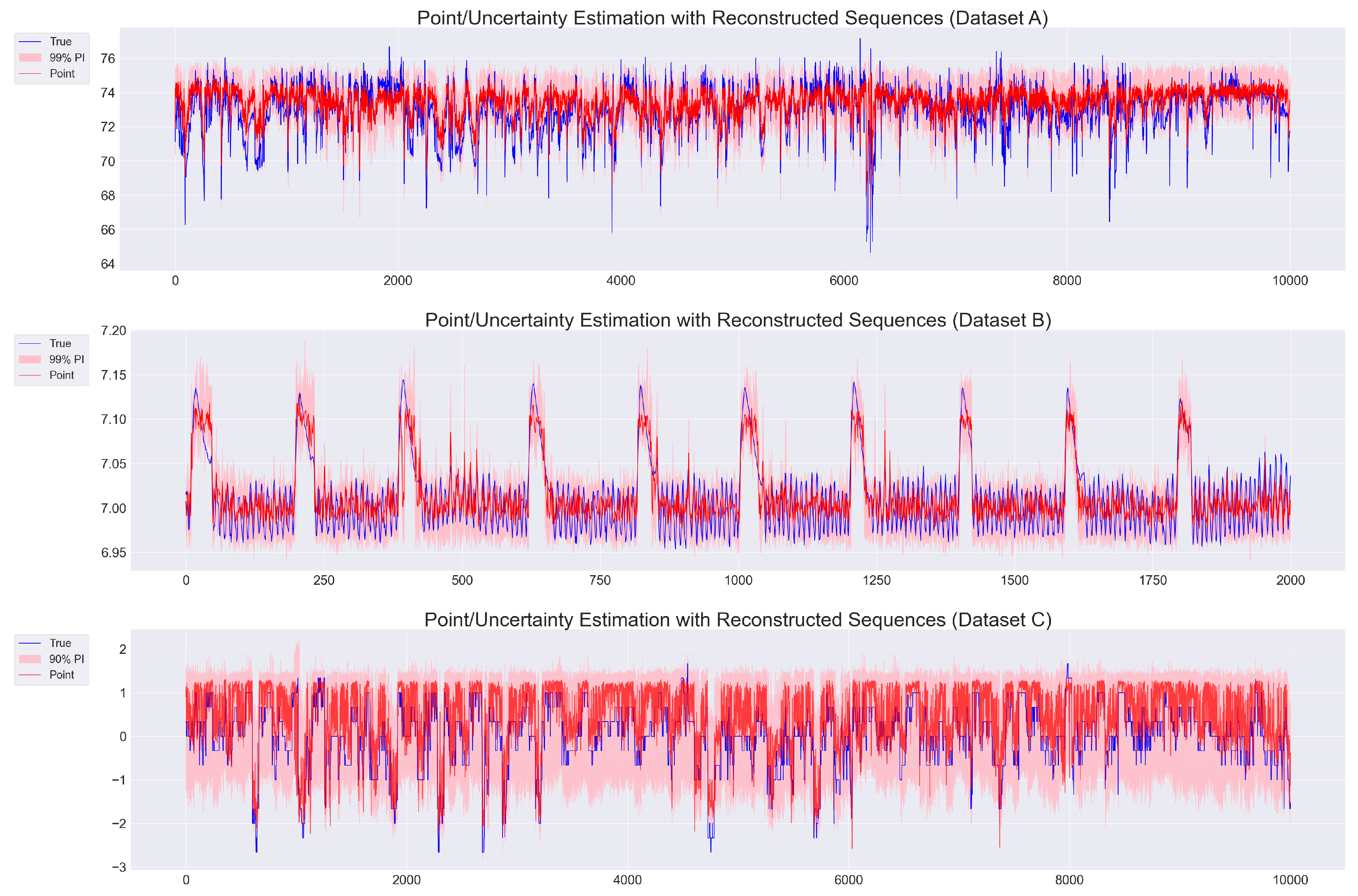
Figure 2.
Forecast-Aware Reconstruction Results based on the best-performing baselines(excluding Mean Reversion) across Datasets A (top), B (middle), and C (bottom). True targets (blue), predictive means (red), and prediction intervals (shaded) are shown.
Figure 2.
Forecast-Aware Reconstruction Results based on the best-performing baselines(excluding Mean Reversion) across Datasets A (top), B (middle), and C (bottom). True targets (blue), predictive means (red), and prediction intervals (shaded) are shown.
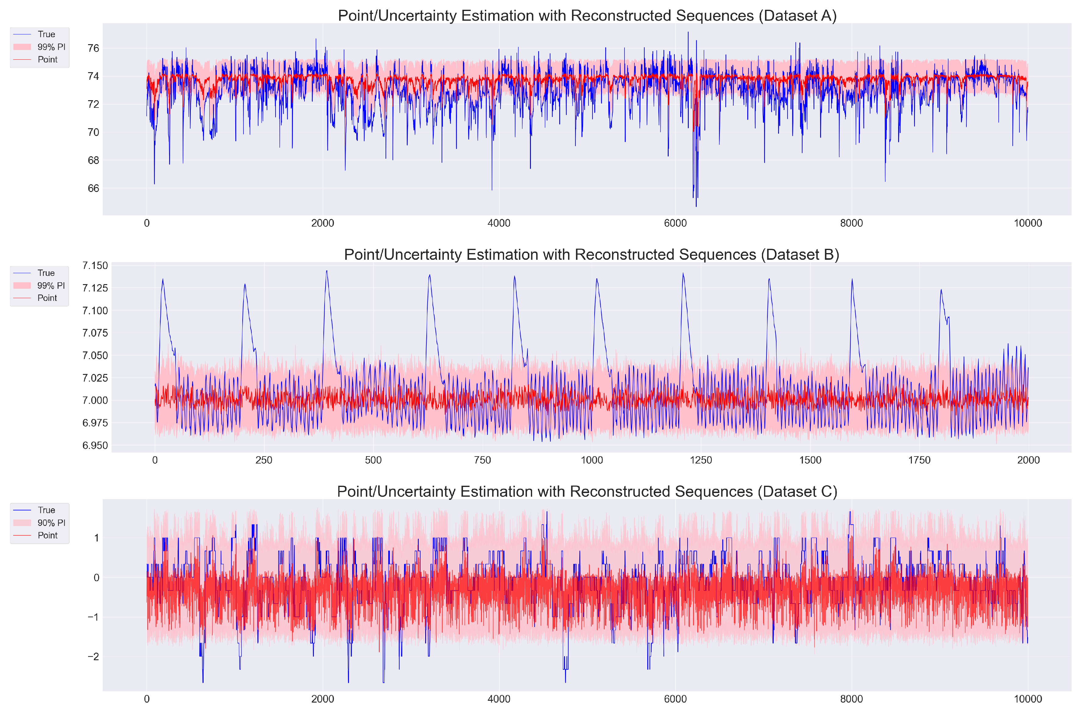

Table 1.
Summary of datasets used in this study, including their domain, size, dimensions, and target variables.
Table 1.
Summary of datasets used in this study, including their domain, size, dimensions, and target variables.
| Dataset | Domain | Raw Size | Shape (Rows × Cols) | Target Variable |
|---|---|---|---|---|
| A (Private) | Sugar | 71,820 | 71,820 × 29 | Brix concentration |
| B (Private) | Bio | 9,201 | 9,201 × 15 | pH concentration |
| C (Public) | Sensor | 99,573 | 99,573 × 25 | Raw Sensor_02 |
Table 2.
Input and target data shapes across three datasets (A, B, and C), including train, validation, and test splits.
Table 2.
Input and target data shapes across three datasets (A, B, and C), including train, validation, and test splits.
| Dataset | Split | Input Shape | Target Shape | Shape Format |
|---|---|---|---|---|
| A | Train | 59,980 × 20 × 28 | 59,980 × 1 | |
| Val | 1,241 × 20 × 28 | 1,241 × 1 | ||
| Test | 10,000 × 20 × 28 | 10,000 × 1 | ||
| B | Train | 6,415 × 85 × 14 | 6,415 × 1 | |
| Val | 531 × 85 × 14 | 531 × 1 | ||
| Test | 2,000 × 85 × 14 | 2,000 × 1 | ||
| C | Train | 83,940 × 60 × 24 | 83,940 × 1 | |
| Val | 5,454 × 60 × 24 | 5,454 × 1 | ||
| Test | 10,000 × 60 × 24 | 10,000 × 1 |
Table 3.
Best-performing models for point prediction and uncertainty estimation across three datasets. It reports the top model for each task along with its respective performance score.
Table 3.
Best-performing models for point prediction and uncertainty estimation across three datasets. It reports the top model for each task along with its respective performance score.
| Dataset | Measure Type | Best Model | Result |
|---|---|---|---|
| A | Balanced-MAE | DeepAR | 0.6673 |
| Unified Uncertainty Score | 0.1776 | ||
| B | Balanced-MAE | MCD CNN-LSTM | 0.1742 |
| Unified Uncertainty Score | DeepAR | 0.2549 | |
| C | Balanced-MAE | MCD CNN-LSTM | 0.3178 |
| Unified Uncertainty Score | DeepAR | 0.3306 |
Table 4.
Reconstruction Model configuration details stage across three datasets.
| Parameter | Dataset A | Dataset B | Dataset C |
|---|---|---|---|
| Model architecture | 128–20–128 | 64–16–64 | 32–8–32 |
| Best epoch (early stopping) | 23/500 | 81/200 | 39/500 |
| Batch size | 64 | 32 | 64 |
| Optmizer | Adam (learning rate ) | ||
| KL Weight | 0.440 | 1.00 | 0.760 |
| Validation MAE Loss | 0.0227 | 0.0376 | 0.0030 |
| Recent Batch Size (N) | 10 | 10 | 30 |
| Target-Aware threshold () | Upper 95th Percentile | Upper 95th Percentile | Lower 95th Percentile |
| Penalty weight (p) | 1.0 | 1.0 | 1.0 |
| Encoder noise (Gaussian std ) | 0.5 | 0.1 | 0.001 |
| Posthoc noise (Gaussian std ) | 0.015 | 0.2 | 0.01 |
Table 5.
Comparison of Forecast-Aware Reconstruction Performance Across Models on Three Datasets. Metrics include MAE and standard deviation of reconstruction error, MAE of first-order differences, and point/uncertainty prediction error. Best results are highlighted in bold.
Table 5.
Comparison of Forecast-Aware Reconstruction Performance Across Models on Three Datasets. Metrics include MAE and standard deviation of reconstruction error, MAE of first-order differences, and point/uncertainty prediction error. Best results are highlighted in bold.
| Model | MAE() | Std () | MAE() | Point / Uncertainty Error |
|---|---|---|---|---|
| Dataset A | ||||
| Proposed | 5.1387 | 11.4274 | 1.8455 | 0.7516/0.1805 |
| Mean Reversion | 4.8363 | 11.4224 | 1.1245 | 1.1228/0.2456 |
| LSTM-CVAE | 5.0352 | 11.9609 | 1.2786 | 1.01691/0.2582 |
| LSTM-WCVAE | 5.2271 | 12.0363 | 2.2277 | 1.1855/0.2801 |
| LSTM-CGAN | 12.6540 | 19.7733 | 4.1229 | 1.6908/0.4080 |
| LSTM-WCGAN | 6.2006 | 14.4517 | 5.5122 | 1.3956/0.3238 |
| Dataset B | ||||
| Proposed | 10.7326 | 15.7482 | 9.8223 | 0.0191/0.2604 |
| Mean Reversion | 8.1444 | 11.4462 | 0.3268 | 0.0304/0.3042 |
| LSTM-CVAE | 9.6854 | 12.8046 | 0.8718 | 0.0299/0.2970 |
| LSTM-WCVAE | 10.0363 | 12.9578 | 1.8012 | 0.0302/0.2915 |
| LSTM-CGAN | 28.0970 | 63.6527 | 11.5516 | 0.0391/0.3864 |
| LSTM-WCGAN | 11.2080 | 15.0513 | 5.9422 | 0.0308/0.3127 |
| Dataset C | ||||
| Proposed | 13.0457 | 27.4023 | 10.2044 | 0.4585/0.2948 |
| Mean Reversion | 9.3925 | 18.1818 | 3.6464 | 0.6926/0.3450 |
| LSTM-CVAE | 7.3437 | 10.2652 | 7.5356 | 0.5039/0.3060 |
| LSTM-WCVAE | 24.2246 | 55.4900 | 7.6082 | 0.5616/0.3831 |
| LSTM-CGAN | 27.6172 | 61.3529 | 7.0803 | 0.7971/0.5492 |
| LSTM-WCGAN | 10.8584 | 23.1551 | 12.3627 | 0.8194/0.4304 |
Table 6.
Evalutation of Batch-wise Temporal Shuffling on Reconstruction and Forecasting Performance Across Different Datasets.
Table 6.
Evalutation of Batch-wise Temporal Shuffling on Reconstruction and Forecasting Performance Across Different Datasets.
| Dataset | MAE() | Std () | MAE() | Point / Uncertainty Error |
|---|---|---|---|---|
| A | / | |||
| B | / | |||
| C | / |
Table 7.
Performance of Candidate Sequence Generation Across Datasets A, B, and C using various target conditions(). Metrics include maximum training MAE, number of sequences passing filtering, target value, best sequence index, and corresponding prediction.
Table 7.
Performance of Candidate Sequence Generation Across Datasets A, B, and C using various target conditions(). Metrics include maximum training MAE, number of sequences passing filtering, target value, best sequence index, and corresponding prediction.
| Dataset | Target Type | Candidate Seqs | Best Seq Index | Best Prediction | ||
|---|---|---|---|---|---|---|
| A | Point | 0.4054 | 822 / 1,000 | 74.25 | 674 | 74.2492 |
| Lower | 812 / 1,000 | 72.10 | 720 | 72.7877 | ||
| Upper | 846 / 1,000 | 75.00 | 4 | 75.0135 | ||
| Min | 867 / 1,000 | 60.08 | 499 | 65.32 | ||
| Max | 877 / 1,000 | 77.37 | 868 | 75.83 | ||
| B | Point | 0.3037 | 899 / 1,000 | 7.0016 | 22 | 7.0015 |
| Lower | 898 / 1,000 | 6.9700 | 281 | 6.9732 | ||
| Upper | 899 / 1,000 | 7.1300 | 593 | 7.1076 | ||
| Min | 898 / 1,000 | 6.9535 | 897 | 6.9726 | ||
| Max | 898 / 1,000 | 7.1527 | 592 | 7.1260 | ||
| C | Point | 0.1271 | 981/1000 | -1.11 | 886 | -1.1123 |
| Lower | 970/1000 | -2.10 | 719 | -2.0997 | ||
| Upper | 987/1000 | 1.05 | 838 | 1.0468 | ||
| Min | 953/1000 | -4.90 | 57 | -4.0312 | ||
| Max | 989/1000 | 1.67 | 649 | 1.3597 |
Table 8.
Performance of Augmented Condition-Aware Sequence Generation Across Multiple Target Types and Datasets (Batchwise-Shuffled).
Table 8.
Performance of Augmented Condition-Aware Sequence Generation Across Multiple Target Types and Datasets (Batchwise-Shuffled).
| Dataset | Target Type | Candidate Seqs | Best Seq Index | Best Prediction | ||
|---|---|---|---|---|---|---|
| A | Point | 0.4054 | 781 / 1,000 | 74.25 | 351 | 74.2512 |
| Lower | 784 / 1,000 | 72.10 | 559 | 72.0962 | ||
| Upper | 796 / 1,000 | 75.00 | 140 | 74.9187 | ||
| Min | 792 / 1,000 | 60.08 | 44 | 65.3882 | ||
| Max | 753 / 1,000 | 77.37 | 671 | 75.7628 | ||
| B | Point | 0.3037 | 869 / 1,000 | 7.0016 | 655 | 7.0015 |
| Lower | 898 / 1,000 | 6.9700 | 868 | 6.9746 | ||
| Upper | 871 / 1,000 | 7.1300 | 189 | 7.1240 | ||
| Min | 868 / 1,000 | 6.9535 | 769 | 6.9747 | ||
| Max | 816 / 1,000 | 7.1527 | 176 | 7.1356 | ||
| C | Point | 0.1271 | 980/1000 | -1.11 | 162 | -1.1083 |
| Lower | 967/1000 | -2.10 | 541 | -2.0978 | ||
| Upper | 985/1000 | 1.05 | 142 | 1.0501 | ||
| Min | 953/1000 | -4.90 | 583 | -4.1495 | ||
| Max | 986/1000 | 1.67 | 647 | 1.3514 |
Disclaimer/Publisher’s Note: The statements, opinions and data contained in all publications are solely those of the individual author(s) and contributor(s) and not of MDPI and/or the editor(s). MDPI and/or the editor(s) disclaim responsibility for any injury to people or property resulting from any ideas, methods, instructions or products referred to in the content. |
© 2025 by the authors. Licensee MDPI, Basel, Switzerland. This article is an open access article distributed under the terms and conditions of the Creative Commons Attribution (CC BY) license (https://creativecommons.org/licenses/by/4.0/).
Copyright: This open access article is published under a Creative Commons CC BY 4.0 license, which permit the free download, distribution, and reuse, provided that the author and preprint are cited in any reuse.


