Submitted:
27 February 2024
Posted:
28 February 2024
You are already at the latest version
Abstract
The statistical analysis of impact of the top 50 solar flares of X-class (1997-2023) on the global seismic activity, as well as on the earthquake preparation zones located in illuminated part of the globe and in the area of 5000 km radius around the subsolar point was carried out. It is shown by a method of epoch superposition that for all cases the increase of seismicity is observed, especially in the region around the subsolar point (up to 38%) during 10 days after the solar flare in comparison with preceding 10 days. The case study of aftershock sequence of strong M=9.1 earthquake (Su-matra-Andaman Islands, 26.12.2004) after the solar flare of X7.2 class (20.01.2005) demonstrated that the number of aftershocks with magnitude M≥2.5 increases more than 20 times after the solar flare with a delay of 7 days. For the case of the Darfield earthquake (M=7.1, 04.09.2010, New Zealand) it was shown that strong solar flares of class X and M probably triggered two strong aftershocks (M>6) with the same delay of 6 days on the Port Hills fault, which is the most sensitive to external electromagnetic impact from point of view of the fault electrical conductivity and orientation. Based on the obtained results the possible application of natural electromagnetic triggering of earthquakes is discussed for a short-term earthquake prediction using confidently recorded strong external electromagnetic triggering impacts on the specific earthquake preparation zones, as well as ionospheric perturbations due to aerosol emission from the earthquake sources recorded by satellites.
Keywords:
solar flare
; geomagnetic field variations
; geomagnetically induced currents
; electromagnetic earthquake triggering
; aerosol emission
; short-term earthquake prediction
1. Introduction
The problem of possible relation of solar activity and the Earth seismicity is discussed over 170 years [1,2,3,4,5,6,7,8,9,10,11,12,13,14,15,16,17,18,19,20], and references therein. Despite a fairly large number of publications devoted to research of the possible influence of the Sun on seismic processes, a final conclusion about a possibility of triggering earthquakes (EQs) by solar flares (SFs) or geomagnetic storms has not yet been made. The results obtained to-date are fuzzy and contradictive, and some authors deny the real existence of interrelation between the processes in the Sun and in the lithosphere resulted in occurrence of EQs [21,22].
It should be noted that all the studies mentioned above employed only a statistical approach to analysis of geophysical and seismological data when the hypothesis of the presence or absence of a possible correlation (positive or negative) between solar activity and Earth's seismicity is tested. The physical mechanisms of solar-terrestrial relations resulted in the possible triggering of EQs were not considered in detail, and their possible existence was only indicated phenomenologically when a statistically significant relationship has been found between solar activity and the response of the Earth's seismicity. Such a simplified approach to the study of the solar-terrestrial relationships may provide false results and incorrect conclusions, as well as no practical recommendations may be proposed for the seismic risk mitigation.
In contrast to pure statistical approach, the study [23] considers a possible physical mechanism of earthquake (EQ) triggering by electromagnetic (EM) impact on the area of EQ preparation due to X-ray radiation of SFs. This idea has been proposed in [16,18], when it was numerically demonstrated that due to interaction of SF X-ray radiation with ionosphere-atmosphere-lithosphere system the strong geomagnetic field pulsations occur resulted in the sharp rise of geomagnetically induced currents (GIC) in the conductive crust faults. It is known that EQ can be triggered by strong variations both of natural and artificial electric currents in the Earth crust as a result of interaction of EM and electric fields with rocks and faults in the Earth's crust under subcritical stress-strain state [24].
The results of numerical studies obtained in [23] using the developed physical model and computer code indicate that after the X-class SF the geomagnetic field pulsations up to 100 nT can occur, and the density of GIC in the conductive layer of the lithosphere can rise to 10-8 - 10-6 A/m2. In this case the current pulse duration is about 100 s, and the duration of the current rise front is ~10 s. These values are 2 - 3 orders of magnitude higher than the average density of telluric currents in the lithosphere [25] and they are comparable with the parameters of electric current pulses generated in the lithosphere (10-7 - 10-8 A/m2) by artificial pulsed sources of electrical energy [24]. It should be noted that the injection of electrical impulses into the Earth's crust in seismically active regions resulted in the EM triggering of weak EQs and the regional spatiotemporal redistribution of seismicity in the Pamirs and Northern Tien Shan. This means that strong SFs providing an energy flux density above 0.005 J/m2 are also capable to trigger EQs in seismically hazardous regions, as was assumed in [18,23,26]. This conclusion is confirmed by cases of observation of magnetic pulses before an EQ [27,28] similarly to the obtained numerical estimates of magnetic pulses generated by X-rays of SF provided telluric current pulses in the conductive layer of the lithosphere, as well as the case of observation of a sharp increase in global and regional seismicity (Greece) after the SF of X9.3 class that occurred on September 6, 2017 [18].
For addition verification of numerical results obtained with application of the physical model of the Sun-Earth interaction [23] we carried out the statistical analysis of impact of the top 50 SFs of X-class on the global seismic activity, the EQs located on illuminated part of the globe, and the EQs located in the area of 5000 km radius around the subsolar point (SSP). We demonstrate that for all cases the increase of seismicity is observed, especially in the region around the SSP (up to 38%) during 6-8 days after the SF. Moreover, we found that the maximum seismic sensitivity to the SF impact is observed in the aftershock area of strong EQ. The case study of aftershock sequence behavior of strong M=9.1 EQ (Sumatra-Andaman Islands, 26.12.2004) after the SF of X7.2 class (20.01.2005) demonstrated that starting from 7th day after the SF the number of aftershocks with magnitude M≥2.5 increases more than 20 times by 8th day and returns to the background level within the following two days. In addition, we consider the case of the Darfield EQ (04.09.2010, M=7.1, New Zealand) with two strong aftershocks (M>6) occurred in the Port Hills fault, which is most sensitive to external EM impact from point of view of the fault electrical conductivity and orientation, with a delay of 6 days after strong SFs of class X and M.
Finally, based on the obtained results we discuss a possibility of application of natural EM triggering of EQs for a short-term EQ prediction using confidently recorded strong external EM triggering impacts on the specific electromagnetically sensitive EQ preparation zones, as well as ionospheric perturbations recorded by satellites due to aerosol emission from the specified EQ preparation zones.
2. Methods of Verification of Hypothesis of Electromagnetic Earthquake Triggering by Strong SFs of X-Class
2.1. Testable Hypothesis of Earthquake Triggering by Strong SFs
In [16,18,23] a possible mechanism of EQ triggering by ionizing radiation of SFs has been proposed. A theoretical model [23] considers a disturbance of electric field, electric current, and heat release in lithosphere associated with variation of ionosphere conductivity caused by absorption of ionizing radiation of SFs. The model predicts generation of geomagnetic field disturbances in a range of seconds to tens of seconds as a result of large-scale perturbation of a conductivity of the bottom part of ionosphere in horizontal direction in the presence of external electric field. Amplitude-time characteristics of the geomagnetic disturbance depend upon a perturbation of integral conductivity of ionosphere. Numerical calculations demonstrated that depending on relation between integral Hall and Pedersen conductivities of disturbed ionosphere the oscillating and aperiodic modes of magnetic disturbances may be observed. For the strong perturbations of the ionosphere conductivities the amplitude of pulsations may obtain ~102 nT. In this case the amplitude of horizontal component of electric field on the Earth surface will obtain 0.01 mV/m and the electric current density in lithosphere may reach 10-6 A/m2. Thus, it was shown that the absorption of ionizing radiation of SFs can result in variations of a density of telluric currents in seismogenic faults comparable with a current density 10-8 - 10-7 A/m2 generated in the Earth crust by artificial pulsed power systems (geophysical MHD generator "Pamir-2" and electric pulsed facility "ERGU-600"), which provide regional EQ triggering and spatiotemporal variation of seismic activity [24]. Therefore, we can expect that the triggering of seismic events is possible not only due to EM impact of the artificial pulsed power sources on the lithosphere, but also due to SFs. Based on the theoretical study above mentioned and numerical results obtained with employment of theoretical model [23] the hypothesis was put forward about the triggering of EQs by strong SFs under certain favorable conditions (electrical conductivity of the fault in the Earth's crust, its orientation relative to the direction of the geomagnetically induced current density vector and the level of stress-strain state of the fault, e.g. its maturity for the dynamic rupture). This study is directed to verification of the hypothesis by analysis of variations of geomagnetic field recorded at INTERMAGNET observatories during strong SFs of X-class, as well as by analysis of seismicity behavior after the flares.
2.2. Analysis of Geomagnetic Field Variations and Seismic Activity during Strong SFs of X-Class
According to theoretical model [23] the SF X-ray radiation will be absorbed in ionosphere resulted in the short-term increase of its conductivity (Figure 1) and disturbances of geomagnetic field in various ranges of periods in the presence of external electric field. It was assumed that the maximal currents in lithosphere are induced by short-period oscillations of the geomagnetic field. The “Earth-ionosphere” resonator generates the geomagnetic field oscillations with periods of 1 to 100s in the process of ionization of the ionosphere by SF radiation with a short front of increase in its amplitude. Considering that the increase in ionosphere conductivity occurs on the illuminated part of the globe, we will analyze the records of INTERMAGNET observatories located there [29] during the SFs from the catalog of the strongest 50 SFs of X-class with intensity of X-ray at peak above 10-4 W/m2 [30]. Coordinates of SSP and area of illuminated part of the globe were determined with application of solar calculator [31].
For verification of the proposed model and obtained numerical results on possible triggering of EQs by SFs [23], an analysis of the Earth seismicity before and after the strongest SFs of class X was carried out. A representative part of the US Geological Survey (USGS) EQ catalogue (M≥4.5) [32] and a catalogue of 50 strongest SFs of class X for the period 1997-2017 [30] were used. The analysis of the possible correlation between SFs and EQs employs the epoch superposition method, when for the time windows of 10 days before and after the arrival of X-rays from the SF to the Earth (~8 min) all EQs occurred in the selected region of the Earth crust were summed up for each day. In accordance with the physical model [23], according to which the maximum burst of telluric currents in the Earth’s crust should occur on the illuminated part of the globe, seismicity of two regions with a center in the SSP and radii of 5000 km and 10000 km was analyzed. The SSP coordinates were determined by the date and time of the SF occurrence.
3. Results of Verification of Hypothesis of Earthquake Triggering by Strong Solar Flares
3.1. Response of Geomagnetic Field to Strong Solar Flare: The Case Study of Solar Flare X5.01 of 2023.12.31
We consider behavior of geomagnetic field (Bx) during strong SF X5.01 occurred on 2023.12.31. The SF occurred at 21:36 UTC, the maximal X-ray flux was reached at 21:55 UTC, and the end of SF was at 22:08 UTC (Figure 2).
According to the model [23] we analyze the recordings of geomagnetic observatories located just near the SSP (23.067°S, 147.733°W) at the distance of 640.96 km and at the distances of 4287.45 to 10003.97 km (on illuminated part of the globe at the moment of the SF), and on the non-illuminated part of the globe at a distance of 15780.24 km from the SSP (Table 1). We consider records of horizontal component Bx of geomagnetic field and its derivative dBx/dt keeping in mind their maximal contribution to GIC in the lithosphere [33]. The magnetograms for different geomagnetic observatories at different distances R from the SSP Bx (a), (c), (e), (g), (i), (k), (m) and dBx/dt (b), (d), (f), (h), (j), (l), (n) for the time around the SF occurrence downloaded from INTERMAGNET site [29] for 2023.12.31 are shown in Figure 3. The SF duration is depicted by shadowed rectangular.
The analysis of recorded variations of geomagnetic field in different parts of the globe (illuminated and non-illuminated) at various distances from the SSP demonstrate that the pulses of Bx and dBx/dt predicted by the model [23] during the SF are observed on the illuminated part of the globe. At the same time there are no pulses of geomagnetic field during the SF of X class on the border of illuminated part (FRD observatory) and on the non-illuminated part. Sharp increase of Bx during the SF is 20-25 nT, and dBx/dt pulsations may obtain 1-4 nT/min. These observations confirm the numerical results obtained with employment of the model [23] that the pulses of geomagnetic field generated by X-ray radiation of the SF and resulted in GIC occurrence in lithosphere are not anticipated at the non-illuminated part of the globe. Thus, the analysis of response of seismic activity to SFs should consider the illuminated part of the globe only. The next question arises: "Are observed pulsed variations of geomagnetic field capable to provoke EQs according to hypothesis of EM triggering of EQs by strong SFs?"
3.2. Seismic Activity before and after Strong SFs of X-Class
For analysis of possible response of seismic activity to the impact of strong SFs we use the representative part (M≥4.5) of the USGS earthquake catalog [32] and a catalogue of 50 strongest SFs of class X [33]. The analysis of the possible correlation between SFs and EQs employs the epoch superposition method, when for the time windows of 10 days before and after the arrival of X-rays from the SF to the Earth all numbers of EQs occurred in the selected region of the Earth crust were summed up for each day. In accordance with the physical model [23], when the maximum burst of telluric currents in the Earth’s crust is anticipated in the illuminated part of the globe, we consider seismic activity in two regions with a center in the SSP and the radii of 5000 km and 10000 km (illuminated part of the globe), and compare the results with seismicity of the whole Earth.
The results obtained are shown in Table 2, where ΣR=5000 is a sum of EQs in the area with a radius of 5000 km around the SSP, ΣR=10000 is a sum of EQs in the area with a radius of 10000 km around the SSP, Σglobal is a sum of EQs for the whole globe, a is the cumulative number of EQs occurring within 10 days after the SF, b is the cumulative number of EQs occurred 10 days before the SF, ΔEQ is an increase in a number of EQs after the SF (%).
The analysis of values of Table 2 demonstrates that according to the physical model [23] and the results of the numerical studies obtained with its application there is a significant seismic response in the illuminated part of the Earth. The maximum increase in the number of EQs (37.88%) is observed in the region with a radius of 5000 km around the SSP. As the radius of the region increases to 10,000 km, which is equivalent to the entire illuminated area of the globe, seismic growth decreases to 13.33%, similar to decrease of geomagnetic field variations (see Section 3.1). In comparison with the global seismicity, the ΔEQ for illuminated part is twice more. The histogram of distribution of a daily number of EQs before and after the SF is shown in Figure 4. It should be noted that the increase in seismicity for the illuminated area of the globe is observed with a delay of 7-8 day after the SF occurrence (Figure 4a,b similar to a few-day delay of response of seismic activity to artificial EM impact on the Earth crust [24].
One of the general conditions for the triggering effect of EM impact on the earthquake preparation zone is the level of stress-strain state of rocks and the crust fault, which, according to the results of laboratory modeling [24], should be 0.98-0.99 of the critical stresses when the dynamic rupture of the fault occurs. The current level of stresses in particular region of the globe can be estimated by indirect signs, e.g. by current seismic activity that is used by methods of mid-term earthquake forecast [34].
However, there are situations when it is possible with a high degree of probability to determine areas where subcritical stresses arise regularly in the Earth's crust. Such areas are aftershock zones of strong EQs. Aftershocks are a sequence of seismic events that occur after a larger main earthquake around the fault zone of the main shock. Aftershocks are a consequence of the stress field redistribution in the Earth's crust after the main displacement along the fault as the result of the main shock. In the aftershock zone the areas occur constantly where the stresses in the Earth's crust will be close to critical values when the rock rupture (aftershock) occurs. Aftershocks become less frequent over time, although they may continue for days, weeks, months or even years e.g., [35]. Thus, due to the indicated stress redistribution in the aftershock zone the areas with a subcritical stress-strain state always appear, which are most sensitive to triggering impacts. In this case, when such an area is located near the SSP during the occurrence of a strong SF, it is possible to anticipate the EM triggering of aftershocks. In this regard, to confirm the hypothesis of EM triggering of earthquakes by SFs, it is quite reasonable to consider the seismic activity in the aftershock zones located near the SSP at the time of the SF occurrence.
As a case study we consider an impact of X7.1 SF of 20.01.2005 on the aftershock zone of the Sumatra-Andaman M9.1 EQ occurred on 26.12.2004. The aftershock zone [36] is covered by the area of 5000 km radius around the SSP of the SF (20.083°S, 77.767°E) of X7.1 class (Figure 5).
The histogram of daily distribution of aftershock number after the main shock of 26.12.2004 is shown in Figure 6. The redistribution of stresses in the crust just after the M9.1 EQ triggered many aftershocks during the first two days (269 and 202), then the daily aftershock number is reduced up to average number of about 20, and after the X7.1 SF, with delay of 6 days, we observe the sharp rise of seismic activity that lasts four days with two peaks of 244 and 240 aftershocks during 27-28 January, 2005. Thus, for the favorable conditions from point of view of generation of geomagnetic field pulsations (for this case recorded at PHU observatory located at a distance of 2933.4 km from SSP and 2248.2 km from the M9.1 EQ epicenter, Figure 7), as well as for the zone with subcritical stress values close to the fault rupture (aftershock zone) we observe clear EQ triggering effect of SF of X7.1 class.
Thus, this case study of aftershock seismicity variation under impact of strong SF confirms that if the aftershock zone is located near the SSP during the occurrence of a strong SF (Figure 5), then we can expect the EM triggering of aftershocks, which can have a magnitude comparable with the main shock, and they are dangerous as well, especially during rescue operations after the catastrophic EQ. For the Sumatra-Andaman M9.1 EQ the maximal magnitude of aftershocks was M6.3.
The obtained results are confirmed by the occurrence of strong aftershocks after SFs of class X and M in the New Zealand region in 2011. A strong M7.1 EQ occurred near Darfield on the South Island of New Zealand [37], which injured about 100 people. After this EQ an aftershock sequence began, which included a strong M6.3 aftershock that occurred on February 21, 2011 and killed 185 people. It should be noted that 6 days before this strong aftershock a SF of class X2.3 occurred (15.02.2011, 01:44-02:06 UTC) when New Zealand was in the central zone of the illuminated part of the globe at a distance of 3853.7 km from the SSP to the M6.3 aftershock epicenter. The EYR observatory (New Zealand) recorded pulsations of geomagnetic field during the SF about 20-25 nT.
According to the results of calculations using the model [23], the current density vector in this region has a southeastern direction and is at a level of 10-7 A/m2, which is comparable to the current density created in the Earth’s crust by an MHD generator, resulted in triggering of EQs at the Northern Tien Shan [24]). For the case of New Zealand, the current density vector coincides with the direction of strike of the Port Hills fault [38], where a strong aftershock occurred. Thus, to trigger an EQ by a SF, the presence of all three conditions of the EM triggering effect was ensured: subcritical stress-strain state fault (EQ aftershock zone), the required level of telluric currents (10-7 A/m2) and the optimal direction of the current density vector (parallel to the direction of the Port Hill fault). It should be noted that this M6.2 aftershock occurred with a delay of 6 days after the SF, which is similar to the response of seismicity to artificial EM influences [24], as well as aftershock activity for the Sumatra-Andaman M9.1 EQ (delay of aftershock response to the SF of 6-8 days). The relationship between these two events (SF and aftershock) is not accidental, since on the same fault there was a repeated strong M6.0 aftershock on 06.13.2011 after M3.64 SF (06.07.2011) with the same delay of 6 days).
4. Discussion
During verification of the physical model [23] by comparison of numerical results on possible triggering of EQs by strong SFs with field observations of variations of geomagnetic field and seismic activity during and after the 50 top strong SFs of X-class we obtained the following results:
- 1)
- Pulsations of geomagnetic field predicted by the model [23] due to interaction of X-ray radiation of SFs with ionosphere are observed during the SF on the illuminated part of the globe. The maximal Bx and dBx/dt pulsations are observed in the area of 5000 km radius around the SSP at the time of SF occurrence. With increasing the area radius, Bx and dBx/dt pulsations decrease and practically disappeared at the border of illuminated part. Such pulsations are not observed on the non-illuminated part of the globe.
- 2)
- The observed sharp variations of geomagnetic field are capable to generate GIC in the conductive elements of lithosphere including seismogenic faults. According to the model [23] these GIC are comparable with a splash of telluric currents generated by artificial pulsed power systems resulted in the EQ triggering and spatiotemporal redistribution of seismicity of Northern Tien Shan and Pamir [24]. Our analysis of seismicity after strong SF confirmed the hypothesis of [24] of EM EQ triggering by SFs (Table 2). For illuminated part within 10 days after the X-class SF seismicity increased in comparison with 10 days before the SF by 13.33 to 37.88% depending on the distance from the SSP. It is much more than for consideration of response of seismicity of the whole Earth. This result confirms the hypothesis [23] of EQ triggering by X-ay radiation of the SF and indicates the incorrectness of pure statistical approach to the study of interrelation of solar and seismic activities without of any physical model explained a possible relation between the process on the Sun and the Earth. For further study it looks reasonable to consider the solar-terrestrial relations based on the physical model [23], or any models considered another physical mechanism of these relations provided refined approach to select the data for statistical analysis. The Physics should be ahead of Statistics.
- 3)
- The next finding of the presented analysis is a response of aftershock area to the impact of SF, where the areas of subcritical stress-strain state appear constantly due to redistribution of the stresses in the crust after the main shock. Based on two case studies of aftershock zones of strong EQs of magnitude M7.1 and M9.1 in New Zealand and Indonesia the clear response of aftershock sequences to the SFs of X-class was discovered. The general feature of this response is a 6 to 8 days delay which may indicate a multi-stage physical mechanism of triggering processes in the crust fault including fluid migration under EM impact that require some time for fluid diffusion into the fault reducing its frictional properties and strength.
In our opinion, the presented results of the analysis of field observations not only confirm the possibility of EQs triggering by strong SFs, but also, taking into account the delay of several days in the response of seismicity to EM impact, indicate the possibility of application of natural EM triggering effects as additional prognostic information for methods of short-term EQ prediction along with other known precursors of strong EQs.
In this case a concept of EQ predictability based on triggering phenomena, which was formulated by Sobolev G.A. [39] may be used. Based on observations of the behavior of seismicity before strong EQs, as well as laboratory studies of the response of acoustic emission (crack formation) from rock samples in a subcritical stress-strain state under external triggering impacts, the following algorithm for short-term EQ prediction based on triggering phenomena was proposed: (a) determining the volume of the unstable zone (a system of unstable zones of various scales; (b) monitoring of triggering effects and assessing their impact on unstable areas; (c) assessing the probability of the location, time and magnitude of the impending EQ.
The first step (a) of this concept can be performed based on various methods for selecting regions with an impending EQ [e.g. [40] and references herein]. For the case of EM impact on the EQ preparation zone in these regions, it is necessary to select additionally the faults in the Earth's crust, taking into account their orientation and electrical conductivity, where the generation of maximum GICs can be expected. It is obvious that the maximum GICs in the fault will be generated in the case when the current density vector is parallel to the fault direction, that contributes to the current concentration in the fault and increases the efficiency of its impact on rocks.
Numerical results [23] demonstrate that the maximum current density values should be observed in the southern hemisphere, while the SSP is located in the northern hemisphere. Thus, the response of seismic activity to a strong SF can be expected with a higher probability in the southern hemisphere. Current density vectors in the northern hemisphere at low and middle latitudes are oriented mainly in the latitudinal direction, and in high latitudes - in the meridional direction. In the southern hemisphere they are usually oriented in the meridional direction. This is important when choosing regions and faults where the response of seismic activity to SFs will be statistically analyzed. In this case, the selection of EQs from seismic catalogs in step (b) should be made only for faults where the expected triggering effect from the EM impact will be maximal. To increase the reliability of the statistical analysis, taking into account the numerical results obtained above, only those regions should be selected where the orientation of the faults in the Earth's crust coincides with the direction of the current density vector. Otherwise, the GIC density generated in the fault may be insufficient to EM triggering of EQ, resulting in the false statistical results and conclusions about solar-terrestrial relationships when seismic activity is analyzed for the entire region with faults of different orientations and electrical conductivity.
Another important aspect when selecting crustal faults that are sensitive to strong variations in space weather is their electrical resistivity, which is usually determined by magnetotelluric (MT) sounding [41]. The results of field studies showed that the San Andreas fault (California, USA) [42] and other major faults, for example, the Alpine fault in New Zealand [43] and the Fraser River fault in British Columbia, Canada [44] have conducting zones with resistivity from 0.8 to 50 Ohm⋅m. At the same time, some large faults demonstrate the presence of both conductive and resistive zones. For example, MT sounding of the Tintina fault in the Northern Cordillera [41] showed that the fault is associated with a resistive zone (>400 Ohm⋅m) of 20 km wide at depths greater than 5 km. The Denali fault in Alaska also has a relatively resistive structure in the upper layers of the Earth's crust [45], and the San Andreas fault in the Carrizo Plain region has a resistive zone in the mid-deep region [46]. The resistivity of these faults varies in the range of ~250 to 10000 Ohm⋅m, and, therefore, the generation of a telluric current pulse due to strong variations in space weather parameters sufficient to trigger an EQ is unlikely or impossible.
Keeping in mind the obtained numerical estimates [23] and their field verification during this study the further detailed correct statistical analysis of solar and seismic activities, firstly, should be based on a physical model of the mechanism of solar-terrestrial relations, and secondly, for the specific model of EM triggering of EQs should be carried out as follows:
a) determination of an unstable area (a fault section in the Earth’s crust) where strong EQs are expected based on existing mid-term methods for selecting seismic-prone regions [40];
b) selection of crustal faults in the regions identified in step (a) that are most sensitive to EM impact in terms of their orientation close to the direction of the GICs density vector, as well as their electrical conductivity;
c) selection from regional seismic catalogs of those EQs that occurred in the faults identified in step (b);
d) correlation analysis of the time of EQ occurrence and variations in space weather parameters to determine the delay time of EQ triggering and threshold values of space weather parameters resulted in the triggering effect in the EQ preparation zone.
As mentioned above, in our opinion, the results obtained, both using the model [23] and field observations employed in this study, can be used in methods for short-term EQ prediction. The algorithm for such a prediction can be as follows. After a strong SF of class X, the areas of possible triggering of EQs are determined, where the impact of the flare can be most effective in terms of medium-term forecast of seismic hazard, electrical conductivity of faults where EQs are expected, and their orientation. In these areas, immediately after the flare, monitoring of other known EQ precursors should be carried out. Based on a multi-parameter approach for analysis of possible precursors a seismic alarm can be issued, taking into account the delay in the response of the EQ preparation zone to the EM triggering effect of several days (6-8 days according to the analysis results obtained above). Obviously, this algorithm is not universal, but can only be used for seismically hazardous areas that are sensitive to EM impacts.
As one of the possible precursors that can be considered after SF in the areas of possible EQ triggering, we propose to consider anomalous variations in ionospheric parameters caused by the emission of aerosols from the EQ preparation zone. To confirm the reliability of this precursor we provide a brief overview of theoretical research and satellite observations below.
It is well known that the process of EQ preparation is accompanied by intensification of emission of soil gases into atmosphere carrying charged soil aerosols. The change of aerosol concentration over the seismic area is determined by satellites measuring the Aerosol Optical Depth (AOD) parameter. This parameter is calculated based on measured data of absorption of solar radiation reflected from the lower atmosphere with a wave length of 550 nm. The authors [47,48,49,50] detected significant AOD increase a few days before EQ that pointed to intensification of aerosol injection into atmosphere. During the similar time period before EQ a rise of quasistatic electric field of 10-2 V/m was detected by satellites in the ionosphere over the epicenter of impending EQ [51,52,53,54,55,56]. Numerous observational data reliably prove the strengthening of electric field in the ionosphere and, at the same time, the absence of a noticeable change in the electric field on the Earth's surface during a few days, that is explained by a model [57,58]. The model relates the increase of electric field with the current rise in the global circuit due to occurrence of electromotive force (EMF) of the external current as a result of injection of charged aerosols into atmosphere (see detailed explanations in [59,60,61,62]). The diagram of the processes in the model is given in Figure 8 where the diagram of a chain of processes resulted in increase of electric field in the ionosphere is shown.
Soli gases (1) carry charged aerosols (2) into the ionosphere which form an external current in the lower atmosphere due to turbulent and convective transport, as well as gravitational precipitation. Inclusion of the external current into the global circuit results in the current increase and, consequently, in the rise of electric filed in ionosphere. An existence of potential barrier at injection of aerosol into atmosphere limits the electric field rise on the earth surface. Perturbation of electric field and current in the global circuit results in numerous plasma and electromagnetic phenomena, which may serve as precursors of increase of seismic activity. The mechanisms of the processes confirmed by field observations are given below.
An increase of electric field in the ionosphere before impending EQ is accompanied by instability of acoustic-gravitational waves (AGW) [63,64]. The critical electric field for the instability occurrence is 6-10 mV/m. The instability results in occurrence of small-scale (about 10 km) heterogeneities of ionosphere conductivity. The high plasma conductivity along the magnetic field results in occurrence of fluctuations of plasma concentrations with an amplitude ∆N/N0 about 1.6 to 16 % elongated along the magnetic field and cross-sectional dimension of about 4 to 40 km.
When the satellite crosses perturbed area of ionosphere with elongated plasma heterogeneities and longitudinal currents with a velocity of 8 km/s, it detects oscillations of plasma density and magnetic field of amplitude about 5 nT with period of 0.4 to 4.0 s. These heterogeneities play a role of whistler ducts [66]. Besides, the small-scale heterogeneities exert an influence on parameters of very low frequency (VLF) transmitter signals recorded by satellites [65]. Blecki et al. [67,68] observed an increase of extra low frequency (ELF) radiation within 1-6 days before strong EQs. This radiation occurs in the ionosphere as a result of the scattering of electromagnetic pulses from lightning strikes on plasma inhomogeneities in the disturbed region [69]. The mechanism of generation of ultralow frequency (ULF) magnetic field due to interaction of background EM field with heterogeneities of ionospheric conductivity is considered in [70]. Polarization currents in the conductivity heterogeneities generate coherent gyro-tropic waves (GTWs), which propagate in the conductive layer. As a result, the magnetic field oscillations occur with a frequency of 0.1 to 10 Hz.
Perturbation of electric current in the global electric circuit is accompanied by ionosphere modification. Laptukhov et al. [71] considered a model of perturbation formation in the D-layer of ionosphere as a result of electric current in the «Earth-ionosphere» layer and electron heating by the current field. The mechanism of disturbance of E-layer of ionosphere as a result of the current rise in the global circuit is considered in [72]. The Ampère force in this layer due to the action of ionospheric wind modifies properties of internal gravitational waves (IGW). This effect results in occurrence of anomalies in VLF/LF signals of transmitters with propagation paths located over seismic area [73–78].
The model of perturbation of F-layer of ionosphere is considered in [79]. The current rise in the global circuit is accompanied by heat release in the E-layer, F-layer heating and plasma drift. These effects result in disturbance of the total electron content.
Occurrence of the external current source in the lower atmosphere as a result of injection of charged aerosols can lead to breakdown electric field at altitudes of 5 to 10 km and electric discharges [80]. The very high frequency (VHF) radiation of these discharges was observed in [81]. The propagation of VHF signals of transmitters beyond the horizon as a result of their scattering by these discharges is considered in [82]. The results obtained are confirmed by observations [83,84].
5. Conclusions
The statistical analysis of impact of the top 50 SFs of X-class (1997-2023) on the seismic activity carried out for verification of the physical model of EM triggering impact of strong SF on the EQ preparation zone confirmed the possibility of EQ triggering on illuminated part of the globe. It is shown that an increase of seismicity is observed, especially in the region around the SSP with a radius of 5000 km (up to 38%) during 10 days after the SF. The case study of aftershock sequence behavior of strong M=9.1 EQ (Sumatra-Andaman Islands, 26.12.2004) after the SF of X7.2 class (20.01.2005) demonstrated that the number of aftershocks with magnitude M≥4.5 increases more than 20 times with delay of 7 days. For the case of the Darfield EQ (M=7.1, New Zealand) it was shown that strong SFs of class X and M probably triggered with observed a delay of 6 days two strong aftershocks (M>6) on the Port Hills fault, which is most sensitive to external EM impact from point of view of the fault electrical conductivity and orientation. Based on the obtained results we conclude that natural EM triggering of EQs may be applied for a short-term EQ prediction using confidently recorded strong external EM triggering impacts on the specific EQ preparation zones, as well as satellite-recorded ionospheric perturbations due to aerosol emission from the EQ preparation zone.
Author Contributions
Conceptualization, V.S. and V.N.; methodology, V.N.; software, V.S.; formal analysis, V.N.; writing—original draft preparation, V.N.; writing—review and editing, V.S. All authors have read and agreed to the published version of the manuscript.
Funding
The study was supported by the Ministry of Science and Higher Education of the Russian Federation (State Assignments of IZMIRAN No. 1021060808637-6-1.3.8, JIHT RAS No. 075-00270-24-00, and IDG RAS No. 122032900167-1).
Conflicts of Interest
The authors declare no conflicts of interest.
References
- Wolf, R. On the periodic return of the minimum of sun-spots: The agreement between those periods and the variations of magnetic declination. Philos. Mag. 1853, 5, 67. [Google Scholar]
- Simpson, J.F. Solar activity as a triggering mechanism for earthquakes, Earth and Planetary Science Letters. 1967, 3, 417-425. [CrossRef]
- Gribbin, J. Relation of sunspot and earthquake activity. Science 1971, 173, 558. [Google Scholar] [CrossRef] [PubMed]
- Meeus, J. Sunspots and earthquakes. Physics Today 1976, 29, 6–11. [Google Scholar] [CrossRef]
- Florindo, F.; Alfonsi, L. Strong earthquakes and geomagnetic jerks: A cause/effect relationship? Ann. Di Geofis. 1995, 38, 457–461. [Google Scholar] [CrossRef]
- Florindo, F.; Alfonsi, L.; Piersanti, A.; Spada, G.; Marzocchi, W. Geomagnetic jerks and seismic activity. Ann. Di Geofis. 1996, 39, 1227–1233. [Google Scholar] [CrossRef]
- Sobolev, G.A.; Zakrzhevskaya, N.A.; Kharin, E.P. On the relation between seismicity and magnetic storms. Izv. Phys. Solid Earth 2001, 37, 917–927. [Google Scholar]
- Zakrzhevskaya, N.A.; Sobolev, G.A. On the seismicity effect of magnetic storms. Izv. Phys. Solid Earth 2002, 38, 249–261. [Google Scholar]
- Sobolev, G.A. The effect of strong magnetic storms on the occurrence of large earthquakes. Izv. Phys. Solid Earth 2021, 57, 20–36. [Google Scholar] [CrossRef]
- Duma, G.; Ruzhin, Y. Diurnal changes of earthquake activity and geomagnetic Sq-variations. Nat. Hazards Earth Syst. Sci. 2003, 3, 171–177. [Google Scholar] [CrossRef]
- Odintsov, S.; Boyarchuk, K.; Georgieva, K.; Kirov, B.; Atanasov, D. Long-period trends in global seismic and geomagnetic activity and their relation to solar activity. Phys. Chem. Earth 2006, 31, 88–93. [Google Scholar] [CrossRef]
- Rabeh, T.; Miranda, M.; Hvozdara, M. Strong earthquakes associated with high amplitude daily geomagnetic variations. Nat. Hazards 2010, 53, 561–574. [Google Scholar] [CrossRef]
- Tavares, M.; Azevedo, A. Influence of solar cycles on earthquakes. Natural Science. 2011, 3, 436–443. [Google Scholar] [CrossRef]
- Shestopalov, I.P.; Kharin, E.P. Relationship between solar activity and global seismicity and neutrons of terrestrial origin. Russ. J. Earth Sci. 2014, 14, ES1002. [Google Scholar] [CrossRef]
- Urata, N.; Duma, G.; Freund, F. Geomagnetic Kp Index and Earthquakes. Open Journal of Earthquake Research, 2018, 7, 39-52. 7. [CrossRef]
- Sorokin, V.M.; Yashchenko A.K., Novikov V.A. A possible mechanism of stimulation of seismic activity by ionizing radiation of solar flares. Earthq. Sci., 2019: 32, 1, 26-34. 32. [CrossRef]
- Marchitelli, V.; Harabaglia, P.; Troise, C.; De Natale, G. On the Correlation between Solar Activity and Large Earthquakes Worldwide. Sci. Rep. 2020, 10, 11495. [Google Scholar] [CrossRef] [PubMed]
- Novikov, V.; Ruzhin, Y.; Sorokin, V.; Yaschenko, A. Space weather and earthquakes: Possible triggering of seismic activity by strong solar flares. Ann. Geophys. 2020, 63, PA554. [Google Scholar] [CrossRef]
- Tarasov, N.T. Effect of Solar Activity on Electromagnetic Fields and Seismicity of the Earth. IOP Conf. Ser. Earth and Env. Sci. 2021, 929, 012019. [CrossRef]
- Anagnostopoulos, G.; Spyroglou, I.; Rigas, A.; et al. The sun as a significant agent provoking earthquakes. Eur. Phys. J. Spec. Top. 2021, 230, 287–333. [Google Scholar] [CrossRef]
- Love, J.J.; Thomas J., N. Insignificant solar-terrestrial triggering of earthquakes. Geophys. Res. Lett. 2013, 40, 1165–1170. [Google Scholar] [CrossRef]
- Akhoondzadeh, M.; De Santis, A. Is the Apparent Correlation between Solar-Geomagnetic Activity and Occurrence of Powerful Earthquakes a Casual Artifact? Atmosphere 2022, 13, 1131. [Google Scholar] [CrossRef]
- Sorokin, V.; Yaschenko, A.; Mushkarev, G.; Novikov, V. Telluric Currents Generated by Solar Flare Radiation: Physical Model and Numerical Estimations. Atmosphere 2023, 14, 458. [Google Scholar] [CrossRef]
- Zeigarnik, V.A.; Bogomolov, L.M.; Novikov, V.A. Electromagnetic Earthquake Triggering: Field Observations, Laboratory Experiments, and Physical Mechanisms - A Review. Izv., Phys. Solid Earth 2022, 58, 30–58. [CrossRef]
- Lanzerotti, L.J.; Gregori, G.P. Telluric currents: The natural environment and interaction with man-made systems. In The Earth's Electrical Environment; The National Academic Press: Washington, DC, USA, 1986; pp. 232–257. [Google Scholar]
- Han, Y.; Guo, Z.; Wu, J.; Ma, L. Possible triggering of solar activity to big earthquakes (Ms ≥ 8) in faults with near west-east strike in China. Sci China Ser G: Phy & Ast. 2004, 47, 173–181. [Google Scholar]
- Scoville, J.; Heraud, J.; Freund, F. Pre-earthquake magnetic pulses. Nat. Hazards Earth Syst. Sci. 2015, 15, 1873–1880. [Google Scholar] [CrossRef]
- Guglielmi, A.V.; Zotov, O.D. Magnetic perturbations before the strong earthquakes. Izv. Phys. Solid Earth 2012, 48, 171–173. [Google Scholar] [CrossRef]
- INTERMAGNET Data Viewer. Available online: https://imag-data.bgs.ac.uk/GIN_V1/GINForms2 (accessed on 1 February 2024).
- Real-time data and plots auroral activity. Available online: https://www.spaceweatherlive.com/en/solar-activity/top-50-solar-flares.html (accessed on 1 February 2024).
- Day and Night World Map. Available online: https://www.timeanddate.com/worldclock/sunearth.html) (accessed on 1 February 2024).
- Search Earthquake Catalog. Available online: https://earthquake.usgs.gov/earthquakes/search/ (accessed on 1 February 2024).
- Thomson, A.W.P.; McKay, A.J.; Viljanen, A. A Review of Progress in Modelling of Induced Geoelectric and Geomagnetic Fields with Special Regard to Induced Currents. Acta Geophys. 2009, 57, 209–219. [Google Scholar] [CrossRef]
- Zavialov, A.D.; Morozov, A.N.; Aleshin, I.M.; Ivanov. S.D.; Kholodkov, K.I.; Pavlenko, V.A. Medium-term Earthquake Forecast Method Map of Expected Earthquakes: Results and Prospects Izv., Atmos. Ocean. Phys. 2022, 58, 908–924. [CrossRef]
- Sedghizadeh, M.; Shcherbakov, R. The Analysis of the Aftershock Sequences of the Recent Mainshocks in Alaska. Appl. Sci. 2022, 12, 1809. [Google Scholar] [CrossRef]
- Araki, E.; Shinohara, M.; Obana, K.; Yamada, T.; Kaneda, Y.; Kanazawa, T.; Suyehiro, K. Aftershock distribution of the 26 December 2004 Sumatra-Andaman earthquake from ocean bottom seismographic observation. Earth Planet Sp. 2006, 58, 113–119. [Google Scholar] [CrossRef]
- Potter, S.H.; Becker, J.S.; Johnston, D.M.; Rossiter, K.P. An overview of the impacts of the 2010–2011 Canterbury earthquakes. Int J Disaster Risk Reduct, 2015, 14, 6-14. [CrossRef]
- New Zealand Active Faults Database. Available online: https://data.gns.cri.nz/af/ (accessed on 5 February 2024).
- Sobolev, G.A. Seismicity dynamics and earthquake predictability. Nat. Hazards Earth Syst. Sci. 2011, 11, 445–458. [Google Scholar] [CrossRef]
- Dzeboev, B.A.; Gvishiani, A.D.; Agayan, S.M.; Belov, I.O.; Karapetyan, J.K.; Dzeranov, B.V.; Barykina, Y.V. System-Analytical Method of Earthquake-Prone Areas Recognition. Appl. Sci. 2021, 11, 7972. [Google Scholar] [CrossRef]
- Ledo, J.; Jones, A.G.; Ferguson, I.J. Electromagnetic images of a strike-slip fault: The Tintina fault-Northern Canadian. Geophys. Res. Lett 2002, 29, 1225. [Google Scholar] [CrossRef]
- Unsworth, M.J.; Malin, P.E.; Egbert, G.D.; Booker, J.R. Internal Structure of the San Andreas Fault Zone at Parkfield, California. Geology 1997, 25, 359–362. [Google Scholar] [CrossRef]
- Ingham, M.; Brown, C. A magnetotelluric study of the Alpine Fault, New Zealand. Geophys. J. Int. 1998, 2, 542–552. [Google Scholar] [CrossRef]
- Jones, A.G.; Kurtz, R.D.; Boerner, D.E.; Craven, J.A.; McNeice, G.W.; Gough, D.I.; DeLaurier, J.M.; Ellis, R.G. Electromagnetic constraints on strike-slip fault geometry - The Fraser River fault system. Geology 1992, 20, 561–564. [Google Scholar] [CrossRef]
- Stanley, W.D.; Labson, V.F.; Nokleberg, W.J.; Csejtey, B.; Fisher, M.A. The Denali fault system and Alaska Range of Alaska: Evidence for underplated Mesozoic flysch from magnetotelluric surveys. Bull. Geol. Soc. Am. 1990, 102, 160–173. [Google Scholar] [CrossRef]
- Mackie, R.L.; Livelybrooks, D.W.; Madden, T.R.; Larsen, J.C. A magnetotelluric investigation of the San Andreas Fault at Carrizo Plain, California. Geoph. Res. Lett. 1997, 24, 1847–1850. [Google Scholar] [CrossRef]
- Qin, K.; Wu, L.X.; Zheng, S.; Bai, Y.; Lv, X. Is there an abnormal enhancement of atmospheric aerosol before the 2008, Wenchuan earthquake? Adv. Space Res. 2004, 54, 1029–1034. [Google Scholar] [CrossRef]
- Okada, Y.; Mukai, S.; Singh, R.P. Changes in atmospheric aerosol parameters after Gujarat earthquake of January 26, 2001. Adv. Space Res. 2004, 33, 254–258. [Google Scholar] [CrossRef]
- Akhoondzadeh, M. Ant Colony Optimization detects anomalous aerosol variations associated with the Chile earthquake of 27 February 2010. Adv. Space Res. 2015, 55, 1754–1763. [Google Scholar] [CrossRef]
- Akhoondzadeh, M.; Chehrebargh, F.J. Feasibility of anomaly occurrence in aerosols time series obtained from MODIS satellite images during hazardous earthquakes. Adv. Space Res. 2016, 58, 890–896. [Google Scholar] [CrossRef]
- Chmyrev, V.M.; Isaev, N.V.; Bilichenko, S.V.; Stanev, G.A. Observation by space-borne detectors of electric fields and hydromagnetic waves in the ionosphere over on earthquake center. Phys. Earth Planet. Inter. 1989, 57, 110–114. [Google Scholar] [CrossRef]
- Gousheva, M.; Glavcheva, B.; Danov, D.; Angelov, P.; Hristov, P.; Kirov, B.; Georgieva, K. Satellite monitoring of anomalous effects in the ionosphere probably related to strong earthquakes. Adv. Space Res. 2006, 37, 660–665. [Google Scholar] [CrossRef]
- Gousheva, M.N.; Glavcheva, R.P.; Danov, D.L.; Hristov, P.L.; Kirov, B.B.; Georgieva, K.Y. Electric field and ion density anomalies in the mid latitude ionosphere: Possible connection with earthquakes? Adv. Space Res. 2008, 42, 206–212. [Google Scholar] [CrossRef]
- Gousheva, M.; Danov, D.; Hristov, P.; Matova, M. Ionospheric quasi-static electric field anomalies during seismic activity August-September 1981. Nat. Hazard. Earth Sys. 2009, 9, 3–15. [Google Scholar] [CrossRef]
- Zhang X.; Chen, H.; Liu, J.; Shen, X.; Miao, Y.; Duc, X.; Qian, J. Ground-based and satellite DC-ULF electric field anomalies around Wenchuan M8.0 earthquake. Adv. Space Res. 2012, 50, 85–95. [CrossRef]
- Zhang, X.; Shen, X.; Zhao, S.; Yao, L.; Ouyang, X.; Qian, J. The characteristics of quasistatic electric field perturbations observed by DEMETER satellite before large earthquakes. J. Asian Earth Sci. 2014, 79, 42–52. [Google Scholar] [CrossRef]
- Sorokin, V.M.; Chmyrev, V.M.; Yaschenko, A.K. Theoretical model of DC electric field formation in the ionosphere stimulated by seismic activity. J. Atmos. Sol. Terr. Phys. 2005, 67, 1259–1268. [Google Scholar] [CrossRef]
- Sorokin, V.M.; Yaschenko, A.K.; Hayakawa, M. A perturbation of DC electric field caused by light ion adhesion to aerosols during the growth in seismic-related atmospheric radioactivity. Nat. Hazards Earth Syst. Sci. 2007, 7, 155–163. [Google Scholar] [CrossRef]
- Sorokin, V.M.; Chmyrev, V.M.; Hayakawa, M. Electrodynamic Coupling of Lithosphere–Atmosphere–Lonosphere of the Earth; Nova Science Publishers: NY, 2015; p. 355. [Google Scholar]
- Sorokin, V.M.; Chmyrev, V.M.; Hayakawa, M. A Review on Electrodynamic Influence of Atmospheric Processes to the Ionosphere. Open J. Earthq. Res. 2020, 9, 113–141. [Google Scholar] [CrossRef]
- Sorokin, V.M.; Hayakawa, M. Generation of seismic-related DC electric fields and lithosphere-atmosphere-ionosphere coupling. Mod. Appl. Sci. 2013, 7, 1–25. [Google Scholar] [CrossRef]
- Sorokin, V.M.; Hayakawa, M. Plasma and electromagnetic effects caused by the seismic-related disturbances of electric current in the global circuit. Mod. Appl. Sci. 2014, 8, 61–83. [Google Scholar] [CrossRef]
- Sorokin, V.M.; Chmyrev, V.M.; Isaev, N.V. A generation model of mall-scale geomagnetic field-aligned plasma inhomogeneities in the ionosphere. J. Atmos. Solar-Terr. Phys. 1998, 60, 1331–1342. [Google Scholar] [CrossRef]
- Chmyrev, V.M.; Sorokin, V.M. Generation of internal gravity vortices in the high-latitude ionosphere. J. Atmos. Solar–Terr. Phys. 2010, 72, 992–996. [Google Scholar] [CrossRef]
- Chmyrev, V.M.; Sorokin, V.M.; Shklyar, D.R. VLF transmitter signals as a possible tool for detection of seismic effects on the ionosphere. J. Atmos. Solar-Terr.Phys. 2008, 70, 2053–2060. [Google Scholar] [CrossRef]
- Hayakawa, M.; Yoshino, T.; Morgounov, V.A. On the possible influence of seismic activity on the propagation of magnetospheric whistlers at low latitudes. Phys. Earth Planet. Inter. 1993, 77, 97–108. [Google Scholar] [CrossRef]
- Blecki, J.; Parrot, M.; Wronovski, R. Studies of electromagnetic field variations in ELF range registered by DEMETER over the Sichuan region prior to the 12 May 2008 earthquake. Int. J. Remote Sens. 2010, 31, 3615–3629. [Google Scholar] [CrossRef]
- Blecki, J.; Parrot, M.; Wronovski, R. Plasma turbulence in the ionosphere prior to earthquakes, some remarks on the DEMETER registrations. J. Asian Earth Sci. 2011, 41, 450–458. [Google Scholar] [CrossRef]
- Borisov, N.; Chmyrev, V.; Rybachek, S. A new ionospheric mechanism of electromagnetic ELF precursors to earthquakes. J. Atmos. Solar-Terr. Phys. 2001, 63, 3–10. [Google Scholar] [CrossRef]
- Sorokin, V.M.; Chmyrev, V.M.; Yaschenko, A.K. Ionospheric generation mechanism of geomagnetic pulsations observed on the Earth’s surface before earthquake. J. Atmos. Solar-Terr. Phys. 2003, 64, 21–29. [Google Scholar] [CrossRef]
- Laptukhov, A.I.; Sorokin, V.M.; Yashchenko, A.K. Disturbance of the ionospheric D region by the electric current of the atmospheric - ionospheric electric circuit. Geomagn. Aeron. 2009, 49(6), 768–774. [Google Scholar] [CrossRef]
- Sorokin, V.M.; Yaschenko, A.K.; Hayakawa, M. Formation mechanism of the lower ionosphere disturbances by the atmosphere electric current over a seismic region. J. Atmos. Solar-Terr. Phys. 2006, 68, 1260–1268. [Google Scholar] [CrossRef]
- Biagi, P.F.; Piccolo, R.; Castellana, L.; Maggipinto, T.; Ermini, A.; Martellucci, S.; Bellecci, C.; Perna, G.; Capozzi, V.; Molchanov, O.A.; Hayakawa, M.; Ohta, K. VLF-LF radio signals collected at Bari (South Italy): A preliminary analysis on signal anomalies associated with earthquakes. Nat. Hazards Earth Syst. Sci. 2004, 7, 685–689. [Google Scholar] [CrossRef]
- Rozhnoi, A.A.; Solovieva, M.S.; Molchanov, O.A.; Hayakawa, M.; Maekawa, S.; Biagi, P.F. Anomalies of LF signal during seismic activity in November–December 2004. Nat. Hazards Earth Syst. Sci. 2005, 75, 657–660. [Google Scholar] [CrossRef]
- Rozhnoi, A.A.; Molchanov, O.A.; Solovieva, M.S.; Gladyshev, V.; Akentieva, O.; Berthelier, J.J.; Parrot, M.; Lefeuvre, F.; Hayakawa, M.; Castellana, L.; Biagi, P.F. Possible seismo-ionosphere perturbations revealed by VLF signals collected on ground and on a satellite. Nat. Hazards Earth Syst. Sci. 2007, 7, 617–624. [Google Scholar] [CrossRef]
- Hayakawa, M.; Surkov, V.V.; Fukumoto, Y.; Yonaiguchi, N. Characteristics of VHF over-horizon signals possibly related to impending earthquakes and a mechanism of seismo-atomospheric perturbations. J. Atmos. Solar-Terr. Phys. 2007, 69, 1057–1062. [Google Scholar] [CrossRef]
- Sorokin, V.M.; Pokhotelov, O.A. The effect of wind on the gravity wave propagation in the Earth’s ionosphere. J. Atmos. Solar–Terr. Phys. 2010, 72, 213–218. [Google Scholar] [CrossRef]
- Sorokin, V.M.; Pokhotelov, O.A. Model for the VLF-LF radio signal anomalies formation associated with earthquakes. Adv. Space Res. 2014, 54, 2532–2539. [Google Scholar] [CrossRef]
- Ruzhin, Y.Y.; Sorokin, V.M.; Yaschenko, A.K. Physical mechanism of ionospheric total electron content perturbations over a seismoactive region. Geomag. Aeron. 2014, 54, 337–346. [Google Scholar] [CrossRef]
- Sorokin, V.M.; Ruzhin, Y.Y.; Yaschenko, A.K.; Hayakawa, M. Generation of VHF radio emissions by electric discharges in the lower atmosphere over a seismic region. J. Atmos. Solar–Terr. Phys. 2011, 73, 664–670. [Google Scholar] [CrossRef]
- Ruzhin, Y.; Nomicos, C. Radio VHF precursors of earthquakes. Natural Hazards 2007, 40, 573–583. [Google Scholar] [CrossRef]
- Sorokin, V.M.; Yaschenko, A.K.; Hayakawa, M. VHF transmitter signal scattering on seismic related electric discharges in the troposphere. J. Atmos. Solar-Terr. Phys. 2014, 109, 15–21. [Google Scholar] [CrossRef]
- Fukumoto, Y.; Hayakawa, M.; Yasuda, H. Investigation of over-horizon VHF radio signals associated with earthquakes. Nat. Hazards Earth Syst. Sci. 2001, 1, 107–112. [Google Scholar] [CrossRef]
- Yasuda, Y.; Ida, Y.; Goto, T.; Hayakawa, M. Interferometric direction finding of over-horizon VHF transmitter signals and natural VHF radio emissions possibly associated with earthquakes. Radio Sci. 2009, 44, RS2009. [Google Scholar] [CrossRef]
Figure 1.
An example of the spatial distribution of the integrated Pedersen (left panel) and Hall (right panel) conductivities in the latitude range -80° - 80° for the universal time 12:00UT. The red vertical line shows the position of the subsolar meridian.
Figure 1.
An example of the spatial distribution of the integrated Pedersen (left panel) and Hall (right panel) conductivities in the latitude range -80° - 80° for the universal time 12:00UT. The red vertical line shows the position of the subsolar meridian.
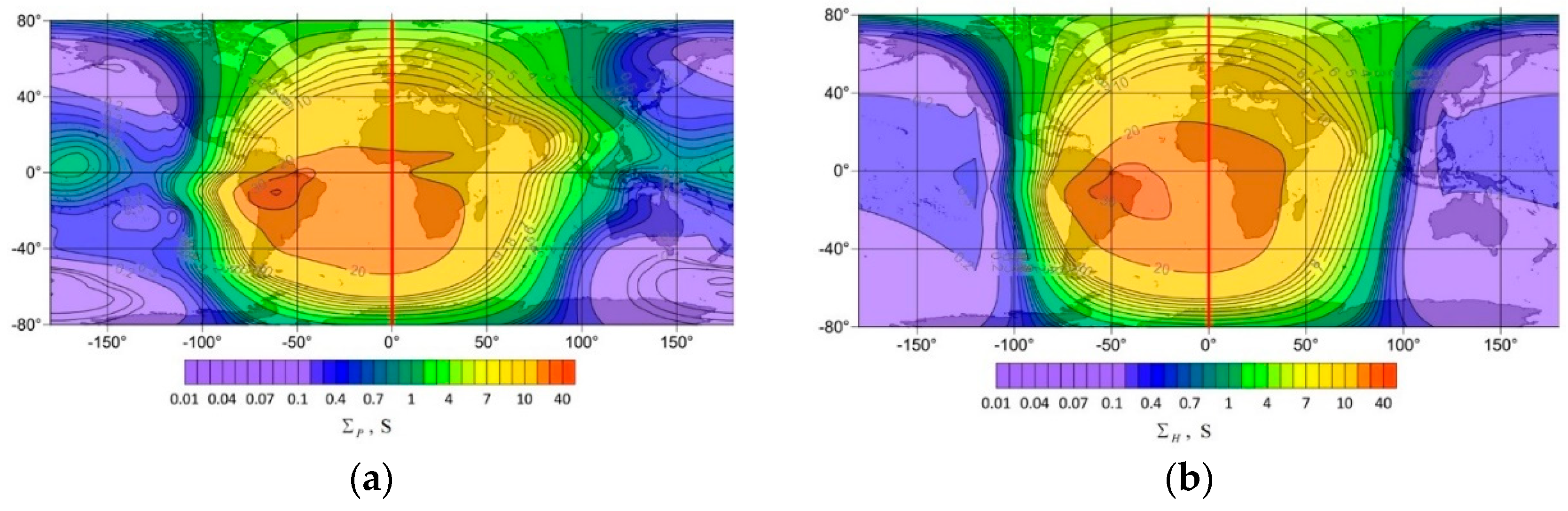
Figure 2.
(a) Location of SSP for X5.01 SF of 2023.12.31 with coordinates 23.067°S, 147.733°W during the peak radiation on 21:55 UTC; (b) GOES X-ray satellite 1-minute solar X-rays average in the 1-8 Angstrom passband [30].
Figure 2.
(a) Location of SSP for X5.01 SF of 2023.12.31 with coordinates 23.067°S, 147.733°W during the peak radiation on 21:55 UTC; (b) GOES X-ray satellite 1-minute solar X-rays average in the 1-8 Angstrom passband [30].
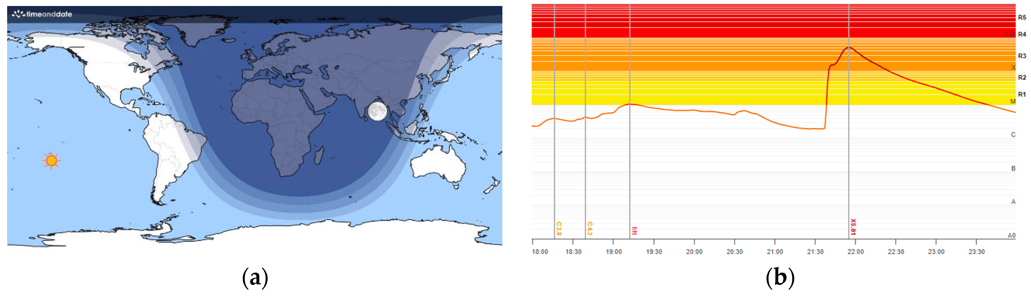
Figure 3.
Variations of geomagnetic field Bx (left panels) and dBx/dt (right panels) recorded at various geomagnetic observatories (Table 1) during the SF of X5.01 class of December 31, 2023: (a), (b) – PPT, R=640.92 km; (c), (d) – EYR, R=4287.45 km; (e), (f) – HON, R=5059.38 km; (g), (h) – CTA, R=6774.29 km; (i), (j) – AIA, R=7388.67 km; (k), (l) - FRD, R=10003.97 km; (m), (n) - ABG, R=15780.24 km. The SF duration is depicted by shadowed rectangular.

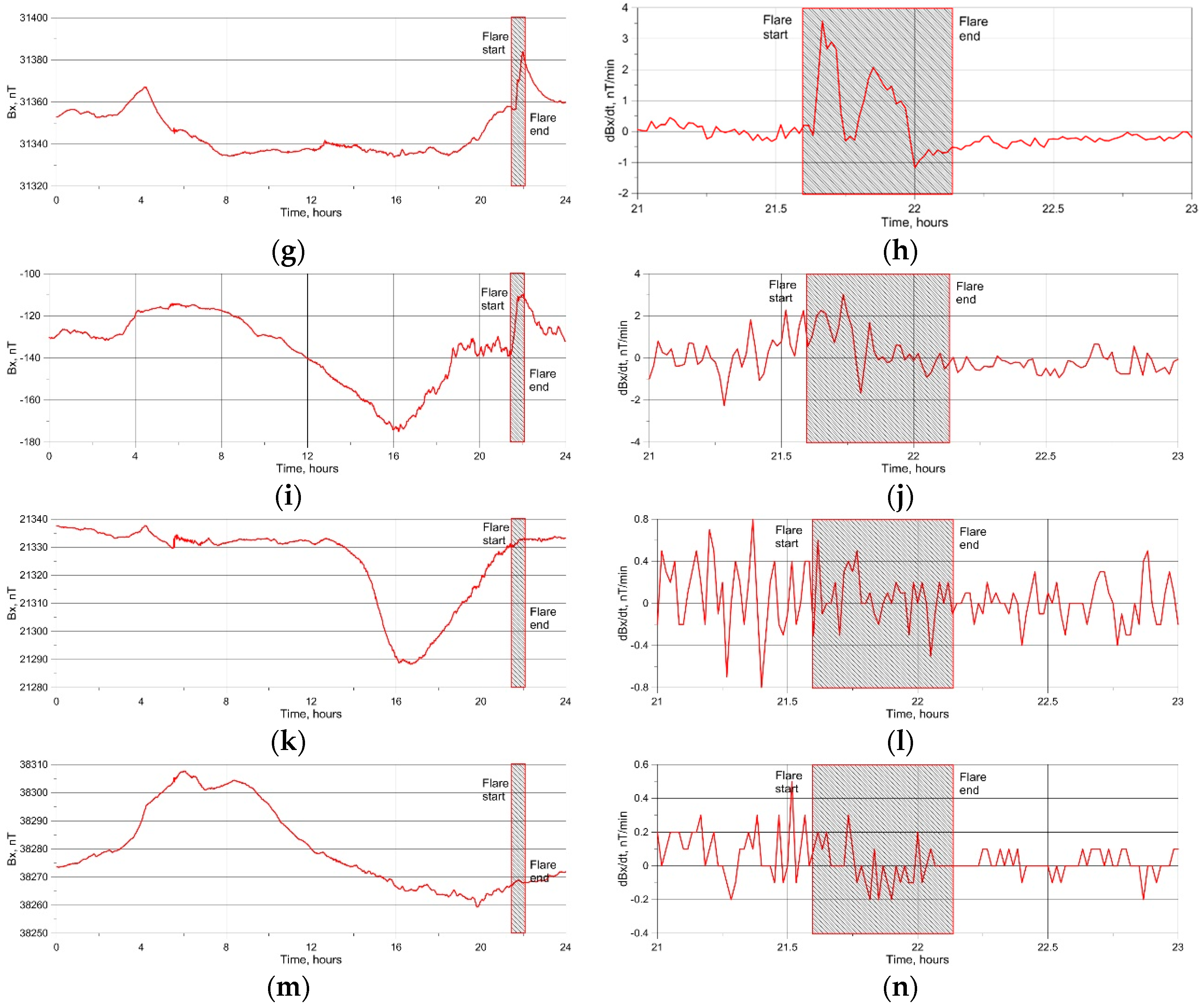
Figure 4.
Seismic activity before and after SF for (a) illuminated part of the globe; and (b) for the area with radius of 5000 km around the SSP.
Figure 4.
Seismic activity before and after SF for (a) illuminated part of the globe; and (b) for the area with radius of 5000 km around the SSP.
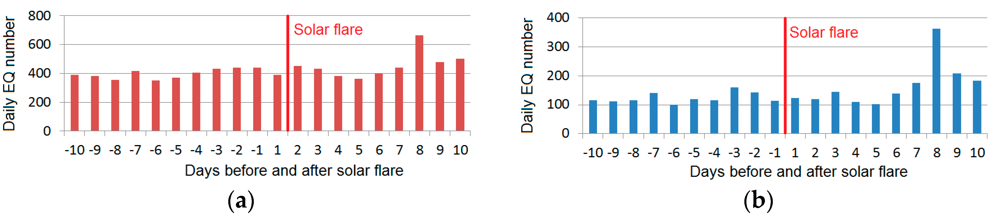
Figure 5.
(a) SSP location (20.083°S, 77.767°E) for the X7.1 SF of 20.01.2005; red circle is the Sumatra-Andaman M9.1 EQ epicenter location (3.295°N, 95.982°E) [31]; (b) Enlarged aftershock zone of Sumatra-Andaman M9.1 EQ of 26.12.2004; red circle is the EQ epicenter located at a distance of 2717.6 km from SSP; grey circles are epicenters of aftershocks (M≥2.5) [32].
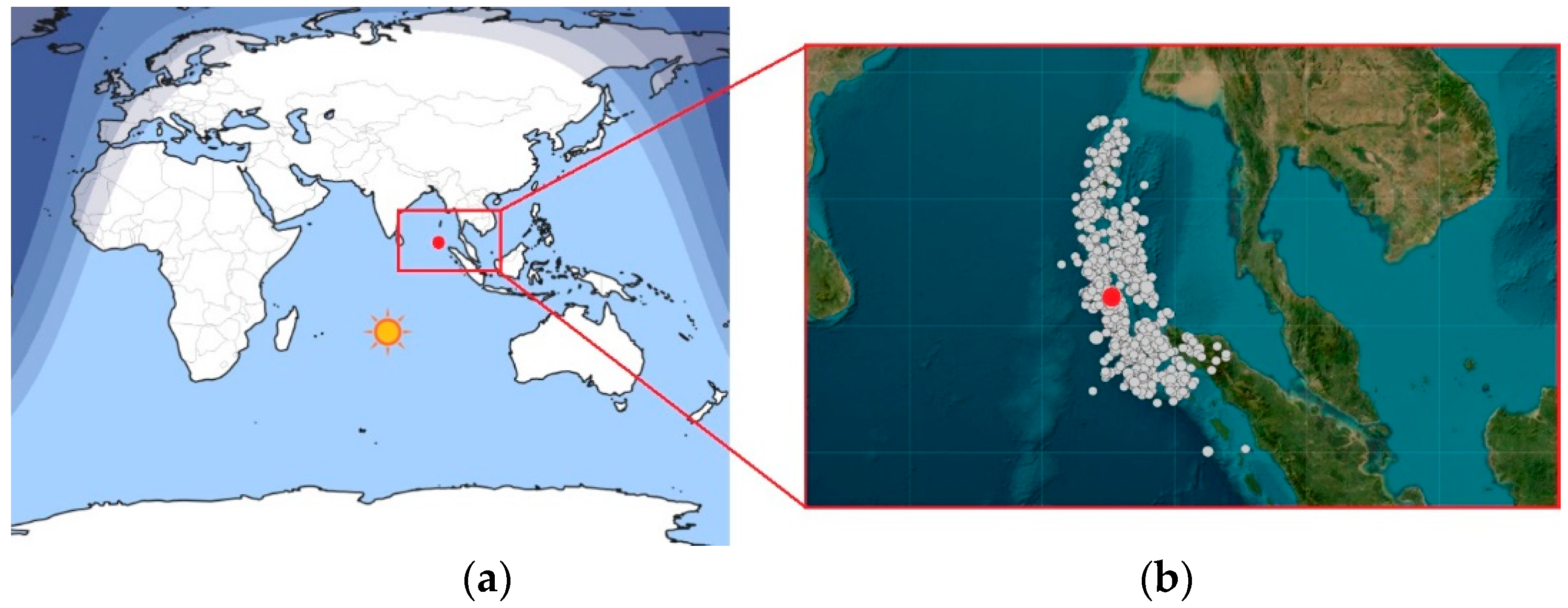
Figure 6.
Daily distribution of aftershock number of Sumatra-Andaman M9.1 EQ (depicted at the left by thick black vertical line). The date of X7.1 SF (20.01.2005) is depicted by thick red vertical line.
Figure 6.
Daily distribution of aftershock number of Sumatra-Andaman M9.1 EQ (depicted at the left by thick black vertical line). The date of X7.1 SF (20.01.2005) is depicted by thick red vertical line.

Figure 7.
Variations of geomagnetic field Bx and (b) dBx/dt recorded at PHU observatory located at a distance of 2933.4 km from SSP and 2248.2 km from the M9.1 EQ epicenter during the SF of X7.1 class of January 20, 2005. The SF duration is depicted by shadowed rectangular.
Figure 7.
Variations of geomagnetic field Bx and (b) dBx/dt recorded at PHU observatory located at a distance of 2933.4 km from SSP and 2248.2 km from the M9.1 EQ epicenter during the SF of X7.1 class of January 20, 2005. The SF duration is depicted by shadowed rectangular.
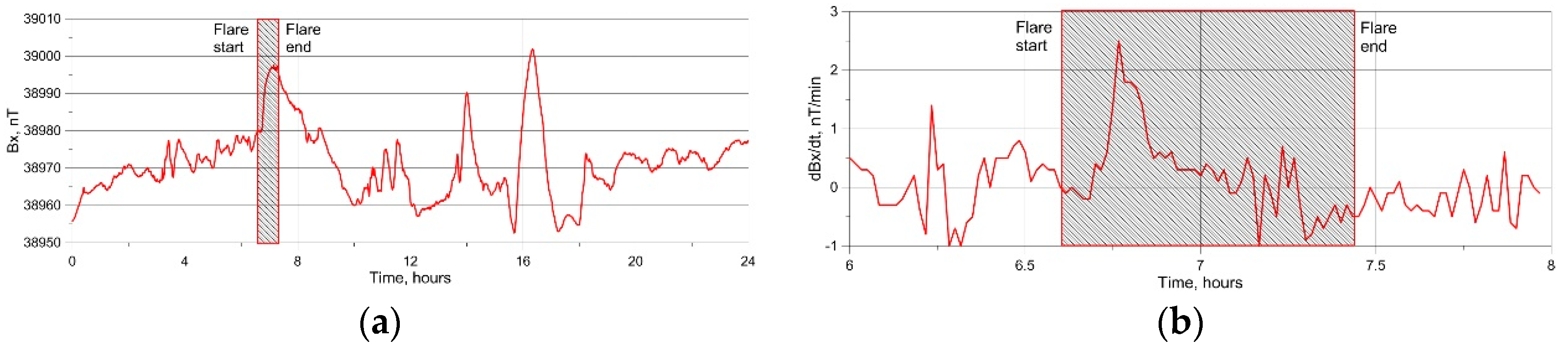
Figure 8.
The model of DC electric field penetration into ionosphere. 1 – soil gases; 2 – charged aerosols injected into atmosphere; 3 – electromotive force in atmosphere; 4 – perturbation of electric field in the global circuit; 5 – conductive layer of ionosphere.
Figure 8.
The model of DC electric field penetration into ionosphere. 1 – soil gases; 2 – charged aerosols injected into atmosphere; 3 – electromotive force in atmosphere; 4 – perturbation of electric field in the global circuit; 5 – conductive layer of ionosphere.
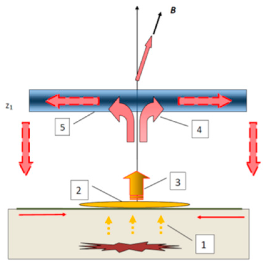

Table 1.
Location of INTERMAGNET observatories with IAGA codes used for analysis of Bx and dBx/dt variations during X5.01 SF on 2023.12.31.
Table 1.
Location of INTERMAGNET observatories with IAGA codes used for analysis of Bx and dBx/dt variations during X5.01 SF on 2023.12.31.
| IAGA Code | Latitude | Longitude | Distance to Subsolar Point R, km |
|---|---|---|---|
| PPT | -17.567 | 210.426 | 640.92 |
| EYR | -43.474 | 172.393 | 4287.45 |
| HON | 21.320 | 202.000 | 5059.38 |
| CTA | -20.090 | 146.264 | 6774.29 |
| AIA | -65.245 | 295.742 | 7388.67 |
| FRD | 38.210 | 282.633 | 10003.97 |
| ABG | 18.638 | 72.872 | 15780.24 |
Table 2.
The number of EQs (M≥4.5) after (a) and before (b) SF at the distance of 5000 km (ΣR=5000), 10000 km (ΣR=10000) from the SSP, as well for the whole globe (Σglobal).
Table 2.
The number of EQs (M≥4.5) after (a) and before (b) SF at the distance of 5000 km (ΣR=5000), 10000 km (ΣR=10000) from the SSP, as well for the whole globe (Σglobal).
| ΣR=5000 | ΣR=10000 | Σglobal | ||||
|---|---|---|---|---|---|---|
| a | b | a | b | a | b | |
| 1667 | 1209 | 4507 | 3977 | 8664 | 8140 | |
| ΔEQ, % | 37.88 | 13.33 | 6.44 | |||
Disclaimer/Publisher’s Note: The statements, opinions and data contained in all publications are solely those of the individual author(s) and contributor(s) and not of MDPI and/or the editor(s). MDPI and/or the editor(s) disclaim responsibility for any injury to people or property resulting from any ideas, methods, instructions or products referred to in the content. |
© 2024 by the authors. Licensee MDPI, Basel, Switzerland. This article is an open access article distributed under the terms and conditions of the Creative Commons Attribution (CC BY) license (http://creativecommons.org/licenses/by/4.0/).
Copyright: This open access article is published under a Creative Commons CC BY 4.0 license, which permit the free download, distribution, and reuse, provided that the author and preprint are cited in any reuse.


