Wide-Angle Repeat Pass Bistatic SAR Interferometry: A Geometrical Introduction

Fabio Rocca

doi:10.20944/preprints202402.1505.v1

Submitted:

26 February 2024

Posted:

27 February 2024

You are already at the latest version

Abstract

Keywords: SAR; interferometry; bistatic

Keywords:

SAR

;

interferometry

;

bistatic

Subject:

Engineering - Other

1. Introduction

Bistatic SAR is a well-established technique, both theoretically and experimentally, and optimal references are widely available such as [1], [2]. Bistatic SAR interferometry has demonstrated its potential in extracting interferograms with minimal temporal decorrelation noise and atmospheric phase screen suppression [3], which are crucial for applications like Digital Elevation Models (DEM) and ground motion measurements. In the bistatic SAR applications mentioned, there must be coherence between the illuminator (transmitter) and the bistatic receiver and thus they are located as close as possible to each other.

Wide-angle bistatic imaging offers advantages like the removal of corner reflector reflectivity and can provide an improvement in the recovery of the object characteristics as, according to diffraction tomography [4,5], the recovered wavenumbers are changed with respect to those obtained using monostatic SAR's. However, as there is no coherence with the wavenumbers recovered by the monostatic SAR, multi-pass interferometry is mandatory thus leading to temporal decorrelation issues. Finally, wide-angle bistatic SAR provides the advantage of offering new Lines of Sight (LOS) directions which, when combined with the monostatic illuminator, might enable a full 3D recovery of slow ground motions [6] including the along-track one, important for seismologists.

Wide-angle bistatic imaging was studied in the evaluation of a companion to the Argentinean SAOCOM L band satellite [7]. A mission for a companion to a Sentinel-1 satellite, namely the ESA mission Harmony, was approved for a launch [8]. This mission involves Sentinel-1 as illuminator and two companions in various relative locations. Among its many goals, Harmony aims to better identify the North-South (NS) motion of the terrain by positioning two companions 300km up and down the track. It should be observed that Sentinel - 1 and also the two companions of the Harmony mission are large satellites and their position along the orbit is and will be very well defined (the radius of the orbital tube is lower than 100m and the distance of the companions controlled to 400m [8].

Aim of this paper is to identify theoretically the limits of the volume in which the companion has to be positioned with respect to the illuminator, to be able to propose much lighter and less controlled receivers. The LOS perturbations are first discussed, emphasizing that only the components of the LOS perturbations that are orthogonal to the LOS will impact the interferometric coherence, as obvious if the diffraction tomography approach is adopted. Then, only the illumination and reception angles are involved and, together with the azimuth and range resolution, define the obtainable common wavenumbers. The fact that indeed the LOS distance change has a very limited impact on interferometry is corroborated by the analyses made.

As the perturbations of the positions of the satellites are easily determined in cartesian geometry, the paper then introduces the rotation matrix needed to move from Cartesian to LOS-aligned coordinates and simply parameterizes the geometry of the wide-angle bistatic SAR. The layover line is identified and the additional phase shifts due to the height of the scatterer is determined as a function of now three baselines (the two orthogonal to the receiver LOS for the receiver and the vertical one for the illuminator). The spectral support and thus the resolution in range and azimuth is then calculated. Then, the coherence of distributed scatterers is evaluated. The analysis is extended to the wavenumber domain. The paper concludes by highlighting that the bistatic wide-angle case is more tolerant of baseline changes due to their statistical combinations, whereas in the monostatic case illuminator and receiver baselines coincide, leading to maximal sensitivity. Finally, the use of bistatic SAR for the determination of the location of interferers is analyzed.

I. LOS distance perturbations

Let us consider the LOS distance

R

between a target and the transmitter and its perturbations due their position changes on the three axes. Indexes

t

refer to the transmitter and

r

to the target

d = \sqrt{{(R + a_{t} + a_{r})}^{2} + {(b_{t} + b_{r})}^{2} + {(c_{t} + c_{r})}^{2}}

Using a series expansion to evaluate the distance changes due to the displacements of both transmitter and target, we notice that different terms have different dependence on

R^{- 1}

. Namely, terms as

b_{t} b_{r}, c_{t} c_{r}

depend on

R^{- 1},

whereas terms as

a_{t} b_{r} (- 2),

b_{t} c_{r} (- 3), a_{t} a_{r} (- 3)

depend on higher powers of the inverse distance, as indicated by the number in parentheses. Then, the perturbations of interest belong only to the two planes orthogonal to the LOS. Indicating with

Q_{t}, Q_{r}

the positions of the transmitter and target (namely the LOS based coordinates are

Q_{t} = (R + a_{t}, b_{t}, c_{t}); Q_{r} = (a_{r}, b_{r}, c_{r}))

then the approximation of the double difference will be of the type:

\frac{\partial^{2} d}{\partial Q_{t} \partial Q_{r}} = \frac{b ₜ b ᵣ + c ₜ c ᵣ}{R} + t e r m s i n R^{- 2}

Now, indicating with

T, R

the 3D vectors of the 2D components of the displacements of transmitter and receiver orthogonal to their LOS and with

P

the target displacement on the ground (again a 2D vector in 3D) we have the formula

d ~ P_{t}^{T} (\frac{T}{R_{t}} + \frac{R}{R_{r}})

(1)

not so far from the monostatic one, and also consistent with the wavenumber approach. However, now the baseline positioned in the horizontal plane may count, and it should be considered in the evaluation of the critical baseline.

We notice now and we will recall later that moving along and across the resolution cell in the ground plane, changes in

b_{r}, c_{r}

will be induced, and thus a linear change of the distance

d_{t}

, and therefore a phase plane will be added to the returns. Another phase plane will be added by the changes of the receiver position and the changes in

d_{r}

. The sum of the two planes is a third plane. The final fringe frequency will be directed along the summed plane gradient, and two different fringe frequencies will be created along the

x, y

axes. As separability applies, a simple calculation will check that now the coherence is the product of the two

s i n c

’s on the two axes.

II. LOS based coordinate systems

We consider now how to move from Cartesian to LOS aligned coordinates and back. For that, we define the direction cosines of the two LOS's (transmitter, receiver). We establish a Cartesian coordinate system with the origin in the nadir of the transmitter, z the height, y the orbit direction and finally x as the ground range. Let θ_t, θ_r be the incidence angles as indicated in Figure 1. Hence, we have that the LOS distance of the transmitter and its direction cosines are:

\begin{matrix} R_{t} & = & \frac{H}{c o s θ_{t}} \\ c o s i n e s : & \frac{H t a n θ_{t}}{R_{t}}; 0; \frac{H}{R_{t}}; \end{matrix}

If the distance of the receiver along the orbit of the receiver is D, then the LOS distance of the receiver and the direction cosines are:

\begin{matrix} R_{r} & = & \sqrt{\frac{H^{2}}{{c o s}^{2} θ_{t}} + D^{2}} \\ c o s i n e s : & \frac{H t a n θ_{t}}{R_{r}}; \frac{D}{R_{r}}; \frac{H}{R_{r}}; \\ θ_{r} & = & a r c c o s \frac{H}{R_{r}} \end{matrix}

For brevity, let us consider the following symbols only dependent on

θ_{t}, D, H .

α = t a n θ_{t}; η = \frac{D}{H}; β = \frac{1}{\sqrt{1 + α^{2}}}; γ = \frac{1}{\sqrt{1 + α^{2} + η^{2}}}; δ = \frac{1}{\sqrt{α^{2} + η^{2}}} R_{t} = \frac{H}{β}; R_{r} = \frac{H}{γ}

(2)

The direction of the bistatic range is the bisector of the two LOS’s and therefore has the direction of their vector sum. Its direction cosines are as follows, where Q is a normalizing factor.

\frac{H t a n θ_{t}}{R_{t} Q} + \frac{H t a n θ_{t}}{R_{r} Q}; \frac{D}{R_{s} Q}; - \frac{H}{R_{t} Q} - \frac{H}{R_{r} Q}

And then they are

\frac{α (β + γ)}{Q}; \frac{η γ}{Q}; - \frac{β + γ}{Q}

Q = \sqrt{{(1 + \frac{γ}{β})}^{2} + {η^{2} γ}^{2}}

The bistatic angle is:

β_{b} = a r c t a n (η β)

(3)

On the ground plane, the direction of the projection of the bisector is,

ϕ = a r c t a n \frac{η γ}{α (β + γ)}

(4)

not orthogonal to the orbit. Further, the angle of the bisector with the z axis, that is always larger than

θ_{t}

is

χ = a r c c o s (\frac{β}{\sqrt{1 + {(\frac{η β γ}{β + γ})}^{2}}})

(5)

We define now the rotation matrix

R_{r}

from the Cartesian coordinates to those that have the LOS of the receiver as first axis, and the second axis in the horizontal plane. Indeed,

η, α

suffice for the description of the matrix; for the transmitter

η = 0

. With some algebra we reach the following result in the case of the LOS of the receiver at a distance

D

from the transmitter:

R_{r} = [\begin{matrix} α γ & η & - 1 \\ - η δ & α δ & 0 \\ - α γ δ & - η γ δ & 1 / δ^{2} \end{matrix}]

(6)

Its transpose will allow to pass from a LOS based coordinate system where it is easy to define the orthogonal plane, to the Cartesian one. Posing

η = 0

, we find the transmitter matrix:

R_{t} = [\begin{matrix} α β & 0 & - β \\ 0 & 1 & 0 \\ - β & 0 & - α β \end{matrix}]

(7)

III. Resolution in bistatic range and cross range

We will now consider the impact of η on the resolution in bistatic range and cross range. Let us consider the ellipse that has foci in source and receiver and passes through the target. If the target moves of a distance δ along the projection of the bisector on the ground, the ellipse will inflate of

δ

sin

χ

where

χ

is the angle of the bisector with the z axis. The travel path will further increase of the factor

2 \cos (\frac{β_{b}}{2}) .

Increasing η, and thus with the bisector moving towards a more grazing incidence, the travel path will globally slightly increase to

2 δ s i n χ c o s (\frac{β_{b}}{2})

.

Expanding in series the previous formula with respect to

η,

the resolution change is approximately proportional to:

r a n g e r e s . c h a n g e : 1 + \frac{3}{16} η^{2}

Looking at the resolution of bistatic images along bistatic cross range we have to evaluate the change in the deflection of the projection of the bisector in the ground plane due to the change in illumination direction from the transmitter. As found in the Appendix the change of the angle with the x axis of the projection of the bisector as a function of the illumination aperture ɛH is decreasing with η and thus we found:

φ = a r c t a n \frac{η γ + β ɛ + γ ɛ - η^{2} γ^{3} ɛ}{- α β - α γ + η α γ^{3} ɛ} = a r c t a n \frac{η γ}{α (β + γ)} + ɛ α \frac{η^{2} β γ^{3} - β^{2} - γ^{2} - 2 β γ}{2 α^{2} β γ + η^{2} γ^{2} + α^{2} β^{2} + α^{2} γ^{2}}

(8)

and the resolution loss with η is proportional to

Cross range res . change : 1 - \frac{15}{16} η^{2}

Hence, we see that the overall areal resolution will decrease with

η .

To summarize, we have seen that indeed the bistatic fast (and slow) time resolutions are slightly higher (and lower) than in the monostatic case. In the fast time case, because the wavenumber modulus, shorter due to the bistatic angle increase, was more than compensated by the more grazing incidence, whereas for the slow time case we have observed a progressively smaller angular excursion for the same illumination slow time.

IV. The layover line

After azimuth focusing, the natural coordinate system will be bistatic-range and azimuth, not orthogonal. All points from the target that are along the line intersection of

- a vertical plane orthogonal to the y axis (constant azimuth)

- the plane tangent to the rotational ellipsoid (with foci in the satellites) that is also orthogonal to the bisector will have approximately the same travel time.

After azimuth and bistatic range focusing, the targets laying on this line will layover into the ground plane. We indicate this as the layover line. The excess phase found in the focused point will depend on the height of the target:

Bistatic geometry: two positions of the receiver are shown. In green the orthogonal baselines, in black the bistatic ground range gradient direction. The angles θ_t, θ_r are those between the LOS’s (the blue lines) and the verticals through source (left) and receivers (right).

The direction cosines of the layover line are

- β; 0; - α β

We find that the slope in the vertical plane is the same of the monostatic one, orthogonal to the transmitter LOS. As the direction cosines of the transmitter LOS are

s i n θ_{t}; 0; - c o s θ_{t};

and those of the layover line are

c o s θ_{t}, 0, s i n θ_{t}

we see that these lines are orthogonal, as in the monostatic case.

V. Phase rotations along the layover line

We can now calculate the phase shifts along the layover line and also the altitude of ambiguity, determining the effect not of the four baselines, but just three as the horizontal baseline of the transmitter is irrelevant, provided that D is calculated relative to the actual position of the illuminator. Let L be the distance from ground of the target, along the layover line. All orthogonal to the LOS’s, the vertical baseline of the transmitter is indicated as B_tv and the horizontal and vertical ones of the receiver are indicated as B_rh, B_rv.

The rotation along the layover line is determined as follows,

φ = \frac{2 π L}{λ H} {[\begin{matrix} β \\ 0 \\ - α β \end{matrix}]}^{T} (β R_{t} [\begin{matrix} 0 \\ 0 \\ B_{t v} \end{matrix}] + γ R_{r} [\begin{matrix} 0 \\ B_{r h} \\ B_{r v} \end{matrix}]) = = \frac{2 π L}{λ H} ({β B}_{t v} + {β γ^{2} B}_{r v} (1 + \frac{α}{δ}) + η {β γ^{2} (α δ - 1) B}_{r h})

(9)

We just notice that for small

η

, the effect of B_rh increases with

η^{3}

, and it is smaller than that of B_rv.

To find the altitude of ambiguity h_amb, it is only necessary to define as L_amb the one that makes the phase shift φ equal to 2π, and then recall that the height is:

h_{a m b} = L_{a m b} s i n θ_{t} .

VI. Distributed scatterers: coherence losses

We have now to consider the effects of bistatic interferometry on distributed scatterers. The first question that we have to consider is that the illuminated data will backscatter at a completely different angle, so that a change in the illumination direction due to the vertical baseline will indeed impact on the scattered spectrum. E analyze now how the baselines effects will combine.

Same vertical plane

For simplicity, let us start with the simplest case: two satellites in the same orbital plane at different heights; indeed, their velocity will be different, but the lower will slowly overtake the upper during the orbital cycle, and in some locations the two may be considered to be at the same azimuth at the same time, repeatedly in every cycle. So, let us consider to have transmitter and receiver in the same vertical plane, illuminating with different incidence and reflection angles a cell of length

L = N δ,

containing

N

scatterers. In the second passage both angles are slightly changed (we reuse some of the symbols, for brevity)

\begin{array}{r} y_{1} & = & \sum_{n = - N / 2}^{N / 2} x_{n} e x p j \frac{2 π δ n}{λ} (s i n θ_{t} + s i n θ_{r}) \\ y_{2} & = & \sum_{n = - N / 2}^{N / 2} x_{n} e x p j \frac{2 π δ n}{λ} (s i n (θ_{t} + σ) + s i n (θ_{r} + α σ)) \end{array}

The cross-correlation of the data will yield the coherence that we wish to calculate, trying to keep it as high as possible. For example, we will calculate if and how we could compensate the baseline of the transmitter with that of the receiver, compensating the angle change in transmission with another complementary change in the reception. The cross-correlation is

\begin{array}{r} σ_{x}^{2} \sum_{n = - N / 2}^{N / 2} e x p j \frac{2 π n δ}{λ} \times \end{array} \times (s i n (θ_{t} + σ) + s i n (θ_{r} + α σ) - s i n θ_{t} - s i n θ_{r})

Expanding in a power series of

σ

and zeroing the constant and the linear term, so that we obtain the observation angles needed for total compensation, we get

α = - \frac{c o s θ_{t}}{c o s θ_{r}}

and then the next term that would lower the coherence is

- \frac{σ^{2}}{2} (s i n θ_{t} + {(\frac{c o s θ_{t}}{c o s θ_{r}})}^{2} s i n θ_{r})

Just to have a number, let us suppose that the upper satellite height is 619km and the incidence angle is

20^{0} .

The lower satellite height is 420km. The illuminated target is at ground range 217 km and the incidence angle of the second satellite is about

27^{0}

. Imposing that the reduction of the coherence be

\frac{2 π n δ}{λ} \frac{σ^{2}}{2} (s i n θ_{t} + {(\frac{c o s θ_{t}}{c o s θ_{r}})}^{2} s i n θ_{r}) = 2.67 σ^{2} \frac{n δ}{λ} < \frac{π}{18}

and with a 3 m cell and

λ = 0.03

we get

σ < \sqrt{\frac{π}{18 * 2.67} * \frac{3 * 2}{300}} = 0.036

so that the baselines could compensate each other as long as they are both contained in a diameter of about

17 k m .

They will not compensate, in general, but the fact that they could is interesting and allows us to sum statistically their effects.

Two vertical planes

Let us now consider the case of two satellites in the same orbit at distance

D

. We have seen before that there are two vertical baselines for the two LOS. How do they combine? Let us consider the two phase-planes describing the distance changes on a square of side

ρ

.

The three baselines will induce three distance change planes, each with different inclination and direction, dependent also on the bistatic angle

β

and the offset D. However, considering the total effect we still have a planar variation along and across the resolution cell. We indicate with

z_{1 i j}, z_{2 i j}

the scatterers within the cell along the

x, y

axes. The cell is

L \times L = N δ \times N δ

and with

p (x, y) = α x + β y

we indicate the total linear change of the distance. Then, we have for the correlation between

z_{1 i j}, z_{2 i j}

in the two passes

z_{2, m n} = z_{1 m n} e x p (\frac{2 π δ}{λ} j (m α + n β))

and the coherence is

γ = \frac{\sum_{m n} z_{1 m n} z_{1 m n}^{*} e x p (- \frac{2 π δ}{λ} j (m α + n β))}{\sqrt{\sum_{m n} {|z_{1 m n}|}^{2} \sum_{m n} {|z_{2 m n}|}^{2}}}

The

x, y

variables can be separated and thus we have, approximately

E [γ] = \frac{N^{2} σ^{2}}{N^{2} σ^{2}} \sum_{m n} e x p (\frac{2 π δ}{λ} j (m α + n β)) = \frac{s i n π μ}{π μ} x \frac{s i n π ν}{π ν}

where

μ, ν

are the fractions of cycles made in the resolution cell by the two frequencies along the two axes.

VII. Calculation of the coherence

Using the matrices introduced for the change of coordinates, we can calculate

μ, ν

in the case of a cell of sides

ρ

directed along the axes. As we have again

\begin{array}{r} R_{r} & = & H \sqrt{1 + α^{2} + η^{2}} \\ R_{t} & = & H \sqrt{1 + α^{2}} \end{array} \begin{array}{r} μ & = & {[\begin{matrix} \frac{ρ}{λ H} \\ 0 \\ 0 \end{matrix}]}^{T} (β R_{t} [\begin{matrix} 0 \\ 0 \\ B_{t v} \end{matrix}] + γ R_{s} [\begin{matrix} 0 \\ B_{r h} \\ B_{r v} \end{matrix}]) \\ μ & = & \frac{ρ}{H λ} (β^{2} B_{t v} + γ^{2} B_{r v} {- η γ}^{2} B_{h r}) \end{array} \begin{array}{r} ν & = & {[\begin{matrix} 0 \\ \frac{ρ}{λ H} \\ 0 \end{matrix}]}^{T} (β R_{t} [\begin{matrix} 0 \\ 0 \\ B_{t v} \end{matrix}] + γ R_{s} [\begin{matrix} 0 \\ B_{r h} \\ B_{r v} \end{matrix}]) \\ ν & = & \frac{ρ α γ δ B_{r h}}{H λ} \end{array}

(10)

we see how the baselines affect the result.

VIII. Azimuth critical baseline

For a simple assessment of the impact of the horizontal baseline we notice as follows. If the ground resolution is say

δ =

3m, the wavefield is decorrelated after an angle

\frac{λ}{δ} = 0.01 r a d

The beam opening is then:

Δ θ = \frac{2 λ}{δ}

The bistatic angle is

β = a r c t a n \frac{D}{R_{t}}

The horizontal critical baseline is then:

\frac{619 * Δ θ}{2 c o s (π / 6)} * \frac{1}{{c o s}^{2} β} = \frac{619}{2 c o s (π / 6)} (1 + \frac{D^{2}}{R^{2}}) * 0.02 > 7.1 k m

As seen previously, the vertical baselines have a bigger impact, so in principle the iso-dispersion volumes are shaped as elongated rugby balls rather than spheres.

IX. Wavenumber shifts: bistatic

The previous analysis was carried out hypothesizing that no interferogram flattening had happened. Then, the additional phase plane due to the baselines operates on the data as an additional phase screen reducing the coherence as the product of the two sinc's, as said.

The situation is different if there is no significant volumetric effect and the local slope is approximately stationary. Then, the interferogram can be "demodulated" times the local fringes, the coherence re-established to 1, but the spectrum of one of the images is shifted along both directions and thus the area of the wavenumbers that have their correspondent in the other image is reduced, as well known from diffraction tomography [4,5]. In other words, the resolution of the interferogram is reduced as part of the spectra will not correlate, being independent as not co-located.

In order to briefly recall the wavenumber's approach, we remember that the analysis start with the hypothesis that the wave-front is locally planar. So, its spherical character is lost. Indeed, in the previous analyses the LOS distance was found to have a minor contribution and used only to calculate the propagation angles, that will be found again in the wavenumber approach. The incident and the reflected wavenumbers

k_{t} {, k}_{r}

have the direction cosines that have already been calculated and length

|k_{t}| = |k_{r}| = \frac{ω}{c} = \frac{2 π}{λ};

The wavenumber of the reflector

k_{o}

is the sum of the incident and reflected wavenumber

|k_{o}| | = |k_{r} + k_{t}| = 2 \frac{ω}{c} c o s (\frac{a r c t a n (η β)}{2})

(11)

and finally, the wavenumber of the target on the ground plane

|k_{g}|

is the projection of

k_{o} .

So we have to multiply times the cosine of the grazing angle i.e. the sine of the angle with the z axis, namely sin

χ

|k_{g}| = | k_{o} | s i n χ = 2 |k_{t}| * \cos (((arctan (η β)) / 2) \sin χ

(12)

All these wavenumbers lay in the target, source, receiver plane. The illuminated wavenumber domain will change with ω as the different frequencies will correspond to different values of λ, and thus a different modulus of k_o. This corresponds to the bistatic range resolution. Notice that this resolution will depend also on η, as the incidence angle of the bisector and thus its wavenumber length will increase with η.

We observe then that also the overall shape of the 2D spectrum is dependent on η. This shape is approximately rectangular if η =0 and if the extension of the illumination slow time is negligible. Increasing the illumination time, it becomes trapezoidal, even in the monostatic case, considering the ensuing non-orthogonality between the LOS’s and the y axis of the orbit.

In the appendix, we calculate the angle with the x axis of the projection of the bisector on the ground plane and its change with the slow time. We see that the extent of the change, i.e. the resolution in the cross-range direction, is slightly dependent on η.We have seen that the projection of the wavenumber on the ground plane will be longer with increasing η, and thus we expect a parallelogram shape of the spectrum, for significant values of η.

In Figure 2 we show some spectra for equal radio frequency bandwidth and illumination duration and, for increasing η, we see that the shape changes into that of a parallelogram.

Then, in order to appreciate the impact of the baselines, we can still recur to the values of μ, ν previously calculated. To do so, we have to consider also the rotation of the angle

ϕ

(eq. 4) so that the phase shifts are oriented along the data spectrum. Then, it is possible to determine the wavenumber shifts along the directions of the spectral parallelograms, the parallelograms superpositions, and the ensuing interferogram resolution changes.

Spectral support for η = 0.5 and two different baselines sets

Superposition of spectral supports for receiver’s baselines in a sphere of rms radius 1km. Left η=0, right η = 0.8

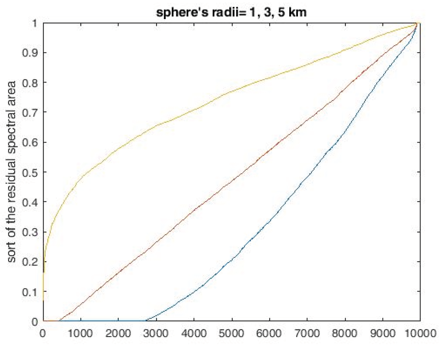
In Figure 2 a, b, I show how the wavenumber domain support changes, as a function of η. The azimuthal resolution is, on purpose, made much lower to be able to identify the two axes. In Figure 3 the superposition is shown of the spectral supports for different baselines, gaussian distributed in a sphere of radius (rms) of 1km and an offset of 0 and 500km. The common part of the spectrum was calculated numerically and it is shown sorted in Figure 4 for rms radii =1;3;5 km.

Sort of the residual interferogram area, for gaussian distributed baselines in a 1, 3, 5 km rms radius sphere; H=619km, D=150km; ρ=3m

X. Localization of interferers

Let us suppose that both satellites can receive at the same time the same interfering signal and the travel time difference can be measured with a precision dependent only on the bandwidth of the interferer. The source is then located on a rotational hyperboloid with foci in both satellites and their junction, namely the common orbit, as the axis. The hyperboloid will intersect the ground with a hyperbola with foci on the nadir of the orbit. As the satellites move along the orbit, so do their images in the ground plane and the intersection of all these hyperbolas all passing through the target will improve the definition of its position.

The rotational hyperboloids

Let

y

be the abscissa on the orbit,

p

the location of the center of the hyperboloid and let the foci be in

p - D / 2; p + D / 2

If

R

is the radius of the cylinder, the equation of the hyperboloid passing through the interferer is

{(\frac{y - p}{a})}^{2} - {(\frac{R}{b})}^{2} = 1

\sqrt{a^{2} + b^{2}} = \frac{D}{2}

Further,

2 a

is the measured difference of the two distances. The interferer is supposed to be on the ground in

y = 0

and

2 a = \sqrt{R^{2} + {(p + D)}^{2}} - \sqrt{R^{2} + {(p - D)}^{2}} \sim 2 p \frac{D}{\sqrt{R^{2} + D^{2}}} \sim \frac{2 p D}{R}

a = \frac{p D}{R}; b \sim \frac{D}{2}; \frac{b}{a} = \frac{D}{2 \frac{p D}{R}} = \frac{R}{2 p}

Let now

H

be the orbit height, and

x

the third coordinate. The rotational hyperboloid has the same equation, but now

R^{2} = H^{2} + x^{2}

{(\frac{y - p}{a})}^{2} - \frac{H^{2} + x^{2}}{b^{2}} = 1

{(\frac{y - p}{a})}^{2} - \frac{x^{2}}{b^{2}} = 1 + \frac{H^{2}}{b^{2}}

The ground hyperbola is

{(\frac{y - p}{a_{1}})}^{2} - \frac{x^{2}}{b_{1}^{2}} = 1

a_{1} = a \sqrt{1 + \frac{H^{2}}{b^{2}}}; b_{1} = b \sqrt{1 + \frac{H^{2}}{b^{2}}}

and thus

x = b_{1} \sqrt{{(\frac{y - p}{a_{1}})}^{2} - 1}

Its slope in the interferer location is

\frac{d x}{d y} = \frac{b_{1}}{a_{1}} \frac{y - p}{\sqrt{(p^{2} - a_{1}^{2} - 2 p y + y^{2})}};

The x direction resolution increases with the width of the angle Δξ covered by all the hyperbolas, namely

Δ ξ \sim \frac{p_{m a x}}{R}

and it is likely to be much lower than that along the y direction.

The situation is opposite in the case that the two satellites have different orbit, and they both receive the interferer. If they are on top of each other, then the hyperboloid has a vertical axis, and the intersection with the ground is a circle passing through the interferer and centered in the common nadir of the two satellites. Now the resolution across the x axis will be maximal, limited only by the interferer band. Similarly, the superpositions of all the circles will better define the position of the interferer along track, but now the along track resolution is much worse.

XI. Conclusions

We have introduced novel formulas that expand upon the calculation of resolution, coherence, altitude of ambiguity, fringe direction, residual interferogram resolution due to the wavenumber shift, specifically addressing bistatic wide-angle radar. In comparison to monostatic systems, bistatic configurations are less susceptible to baseline changes. This reduced sensitivity is attributed to the random combination of three baselines in bistatic setups, which effectively mitigates their impact on the data quality. Further, bistatic systems yield a partial identification of the positions of interferers.

Acknowledgment

The author wishes to thank the Agenzia Spaziale Italiana for the proposal of the theme of the research and the colleagues of the Mission Advisory Group for Platino, namely Proff. Antonio Moccia, Daniele Riccio, Gianfranco Fornaro, and Stefano Perna for many helpful discussions.

Appendix

We calculate the deflection of the projection of the bisector, if the illuminator moves of a length ɛH along the orbit. The transmitter, receiver, target position vectors are:

\begin{array}{r} P_{t} & = [\begin{matrix} 0 \\ ε \\ H \end{matrix}] \end{array} \begin{array}{r} P_{r} & = [\begin{matrix} 0 \\ D + ε \\ H \end{matrix}] \end{array} \begin{array}{r} P_{t} & = [\begin{matrix} H α \\ 0 \\ H 0 \end{matrix}] \end{array}

The incident and reflected vectors are

\begin{array}{r} P_{t} - T & = [\begin{matrix} - H α \\ ε \\ H \end{matrix}] \end{array} \begin{array}{r} P_{r} - T & = [\begin{matrix} - H α \\ D + ε \\ H \end{matrix}] \end{array}

The sum of the two direction cosines is

\begin{array}{r} B & = \frac{1}{Q_{t}} [\begin{matrix} - H α \\ ε \\ H \end{matrix}] & + \frac{1}{Q_{r}} [\begin{matrix} - H α \\ D + ε \\ H \end{matrix}] \end{array} \begin{array}{r}  \end{array}

and to the first order in ɛ

B = β [\begin{matrix} - α \\ ε \\ 1 \end{matrix}] + γ (1 - ε η γ^{2}) [\begin{matrix} - α \\ η + ε \\ 1 \end{matrix}]

The angle with the x axis is:

\begin{array}{l} φ (ɛ) = \arctan \frac{η γ + β ɛ + γ ɛ - η^{2} γ^{3} ɛ}{- α β - α γ + η α γ^{3} ɛ} = \\ = - \arctan \frac{η γ}{α β + α γ} + \frac{ɛ}{α} (1 - \frac{η^{2} γ^{2} (1 + α^{2} β γ)}{{(α (β + γ))}^{2}}) \\ (A 1) \end{array}

References

R. Wang, Y. Deng: Bistatic SAR System and Signal Processing Technology, Springer Singapore, 2018.
G. Krieger, Bistatic and Multistatic SAR: State of the Art and Future Developments, Youtube Webinar.
G. Krieger; A. Moreira; H. Fiedler; I. Hajnsek; M. Werner; M. Younis; M. Zink TanDEM-X: A Satellite Formation for High-Resolution SAR Interferometry, IEEE Transactions on Geoscience and Remote Sensing, 2007, Vol. 45, 11.
Wu, R. S. and M. Nafi Toksöz. "Diffraction tomography and multisource holography applied to seismic imaging." Geophysics 52 (1987): 11-25. [CrossRef]
F. Gatelli, A. Monti Guarnieri, F. Parizzi, P. Pasquali, C. Prati and F. Rocca, "The wavenumber shift in SAR interferometry," in IEEE Transactions on Geoscience and Remote Sensing, vol. 32, no. 4, pp. 855-865, July 1994. [CrossRef]
F Rocca: 3D motion recovery with multi-angle and/or left right interferometry, Proceedings of the third International Workshop on ERS SAR, 2003.
N. Gebert, B. Carnicero Dominguez, M. W. J. Davidson, M. Diaz Martin and P. Silvestrin, "SAOCOM-CS - A passive companion to SAOCOM for single-pass L-band SAR interferometry," EUSAR 2014; 10th European Conference on Synthetic Aperture Radar, Berlin, Germany, 2014, pp. 1-4.
Harmony: EARTH EXPLORER 10 CANDIDATE MISSION: HARMONY REPORT FOR MISSION SELECTION ESA – EOPSM - HARM-RP-4129 Issue/Revision 1.1 Date of Issue 30/06/202.

Figure 1.

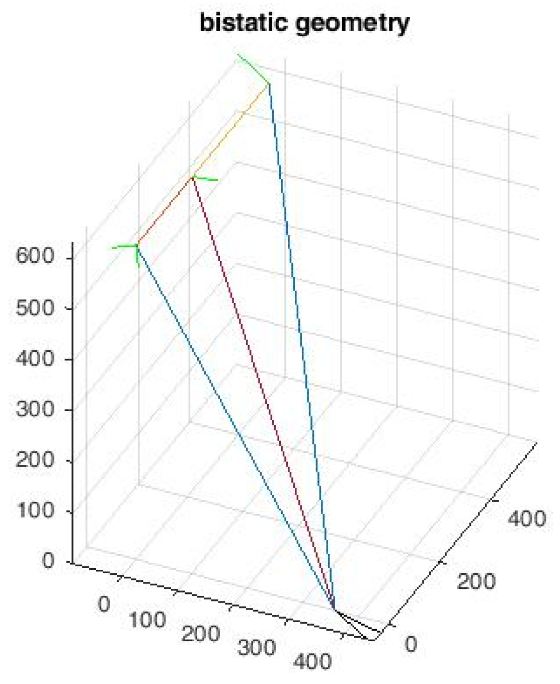
Figure 2.

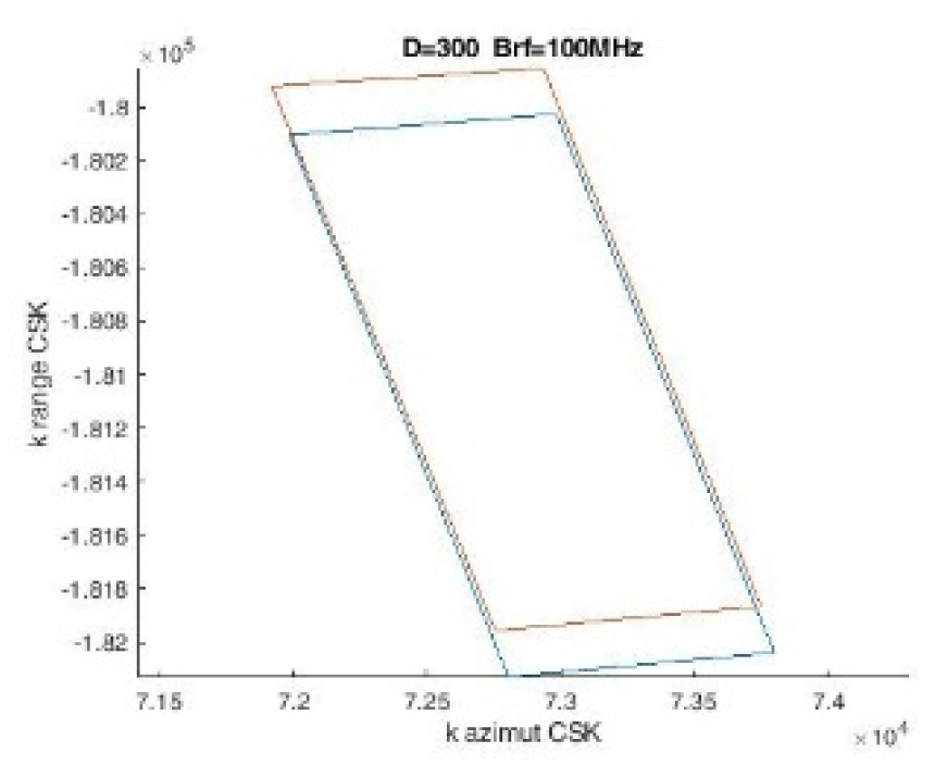
Figure 3.

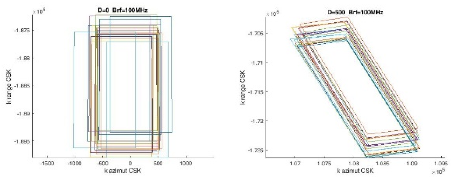
Figure 4.

Disclaimer/Publisher’s Note: The statements, opinions and data contained in all publications are solely those of the individual author(s) and contributor(s) and not of MDPI and/or the editor(s). MDPI and/or the editor(s) disclaim responsibility for any injury to people or property resulting from any ideas, methods, instructions or products referred to in the content.

© 2024 by the authors. Licensee MDPI, Basel, Switzerland. This article is an open access article distributed under the terms and conditions of the Creative Commons Attribution (CC BY) license (http://creativecommons.org/licenses/by/4.0/).

Copyright: This open access article is published under a Creative Commons CC BY 4.0 license, which permit the free download, distribution, and reuse, provided that the author and preprint are cited in any reuse.