Gleason Score Prediction for the Severity of Prostate Metastasis Using Machine Learning

1. Introduction

Cancer is among the main causes of death worldwide. One of the most common cancers that affect men worldwide is prostate cancer with incidence; 1.276 million new cases were diagnosed in 2019. To date, most cancer studies have concentrated on finding biomarkers that enable differentiating malignant tumors from benign ones.

More recent studies, though, have focused on specific clinical aspects of tumors, such as recurrence, progression, survivability, and metastasis, among others. In the 1950s, Pierre Denoix devised a system that categorizes solid tumors into different stages. The classification (TNM) of cancer progression is done by utilizing (T) the extension and the size of the main tumor, (N) the lymphatic involvement, and (M) the metastasis levels. Researchers focused on identifying gene expression patterns that correlate with disease progression, and can be used as predictive tools for patient treatment and outcome. Moreover, advances in next-generation sequencing (NGS) technology have made genomic data analysis widely available. The output of NGS sequencers requires preprocessing algorithms to do things such as align the reads to a reference human genome and assemble them into transcripts. Many genomic tools that align the RNA-Seq reads to the human genome have been proposed, especially BLAST is one of the first tools developed to align reads. TopHat2 is a widely used, open-source tool that incorporates Bowtie sequence alignment to align reads. STAR is the fastest RNA-Seq sequence alignment algorithm to date, although it requires huge computational resources to perform efficiently. Based on the need for understanding the biological basis of the visual Gleason microscopic assessment.

The Gleason score is a pathological grading system to examine the potential aggressiveness of the disease in the prostate tissue. Advancements in computing and next-generation sequencing technology now allow us to study the genomic profiles of patients in association with their different Gleason scores more accurately and effectively. This score is calculated by adding two numbers: the most common pattern of the tumor cells is used as the first number, while the second number corresponds to the next most common pattern. Each individual score varies from 3 to 5, depending on the aggressiveness of the tumor, where the highest score means the most aggressive form of cancer.

In addition to radiation therapy, which has improved survival rates through the development of equipment and combination with hormonal therapy, the development of new drugs, such as androgen signaling target drugs and chemotherapeutic agents, continues to reduce mortality rates associated with single and combined therapy. To facilitate early diagnosis and to avoid unnecessary prostate biopsies, multipara metric magnetic resonance imaging (mpMRI) using a Prostate Imaging-Reporting and Data System (PI-RADS)6 and biomarkers such as free prostate-specific antigen (PSA), total/free PSA ratio and 4Kscore,7 prostate health index,8 and PCA3 (prostate cancer antigen 3)9 may be used to diagnose prostate cancer. The developed techniques of surgery, medicine, and diagnostic tools could help to reduce mortality of prostate cancer.

Recently, artificial intelligence technology and machine learning methods have been applied to analyze large amounts of data the medical field, and their adequacy and usefulness in diagnosis are increasing. Analysis using a combination of machine learning methods and mammograms has led to an accurate diagnosis of breast cancer, and an automatic grading system has been applied to determine the Gleason grade of prostate cancer using histopathological images. Thus, in this study, we will evaluate the applicability of machine learning methods that combine data on age and PSA levels in predicting prostate cancer.

1.1. Problem Statement and Motivation

Gleason grading is associated with substantial interobserver variability, resulting in a need for decision support tools to improve the reproducibility of Gleason grading in routine clinical practice. While there are several methods to detecting prostrate metastasis with good performance on Gleason score calculation and prediction such as prostate-specific antigen (PSA) blood test, a digital rectal exam (DRE), biopsy methods etc. drawbacks associated with these current systems have motivated further research into improvement in the Gleason score prediction processing system using machine learning.

The first drawback is that some of these methods have varying cut-off point on severeness detection. The prospect of having prostate cancer goes up as the PSA level goes up, however no set cutoff point can tell for sure if a man has prostate cancer or not.

Second drawback is that some of these methods can be less effective and are often not comfortable especially when DRE is the adopted method.

Lastly, non-standardized Gleason score from urologist after biopsy have been carried out can lead to under or over treatment of the patients.

Machine learning and deep learning are approach for analyzing medical images. Using deep learning to assess biopsy images results may improve the identification of salient characteristics in the images which could enhance the Gleason score prediction and automate prediction process even at the absence of enough specialists. However, training a deep neural network to achieve this goal would require a large number of expertly labelled images.

1.2. Research Aim and Objectives

The aim of this study is to evaluate the ability of machine learning and deep learning system (DLS) to automate the grading of diagnostic prostate biopsy specimens through the following objectives:

• Train and evaluate a deep learning architecture on the MRI to predict Gleason score.
• Examine the need for transfer learning approach to overcome the issue of more data in deep learning towards achieving better accuracy at Gleason score prediction.
• Improve on the existing ways of deploying Gleason score predicting system for clinical decision making.

1.3. Scope and Limitations

We expect this decision support system to help pathologists to cut back the chance of over-or under-diagnosis by providing pathologist-level second opinions on the Gleason score when diagnosing prostate biopsy, and to support analysis on glandular carcinoma treatment and prognosis by providing consistent diagnosing fully based on the standards of artificial intelligence. However, the result of the system on each biopsy should rather been seen as the probability of obtaining the predicted Gleason score and not the exact Gleason score for the sample tissue.

Also, the generality of the deployed model is limited to samples that are carefully preprocessed as the training data with a tolerance level of 0.3. The author assumptions on properly captured data are that the source of the data and labelling processes have carefully done by the providing institutes ( Karolinska Institute and Radboud University Medical Center)

1.4. Structure of dissertation

The rest of the dissertation is organized as follows. Chapter 2 reviews literature relating to Machine Learning Approaches for the Prediction of Severity of Prostate Metastasis using the Gleason score. Chapter 3 gives an overview of the methodology used to meet the objectives of the study. Chapter 4 entails evaluating the outcome of the trained deep learning model and deployment options including SaaS. Chapter 5 investigates deep learning techniques for model improvement.

2. Literature Review

This chapter reviews literature related to the epidemiology and pathology of cancer with special attention to prostate cancer metastasis, as well as existing methods used to detect the severeness of prostate cancer. Artificial intelligence approach to Gleason scores prediction and grading system for prostate cancer through the use of biomedical image analysis which could be used to improve and automate the Gleason score calculation. Literature related to existing alternative methods was also reviewed, and the development areas in these new approaches highlighted. Special attention is given to the existing machine learning paradigm and frameworks of the web-based Gleason score prediction for prostate cancer metastasis severity detecting tool currently in development.

2.1. Epidemiology and pathology of prostate cancer metastasis

Cancer is a massive cluster of diseases which will begin in nearly any organ or tissue of the body once abnormal cells grow uncontrollably, transcend their usual boundaries to invade neighboring organs of the body and/or unfold to completely different organs. The latter method is named metastasizing and may be a major reason behind death from cancer. in line with the World Health Organization (WHO), Prostate cancer is the fourth commonest cancer overall and also the second commonest cancer in men. There are approximately 1.1 million men worldwide diagnosed with prostate cancer in 2012 (which accounted for 15% of all cancer incident cases in men), with almost 759 000 of the cases (70%) occurring in more developed regions. Prostate cancer is the second commonest reason behind male cancer deaths in Western countries (Roberts et al., 2000). Its incidence varies by a factor of more than 25 worldwide and the rates square measure highest in Australia/New island and North America (with 2012 age-standardized incidence rates of 111.6 and 97.2 cases per 100000 men, respectively) and in the western and northern Europe geographical regions, because the adoption of prostate-specific substance (PSA) testing and the ensuant diagnostic test (biopsy) has become widespread in those regions. With over 300 000 deaths in 2012, prostate cancer is the fifth leading reason behind death from cancer in men which account for 6.6% of all cancer deaths in men.

Figure 2.1. Estimated age-standardized rates (World) in the world (per 100 000).

Figure 2.1. Estimated age-standardized rates (World) in the world (per 100 000).

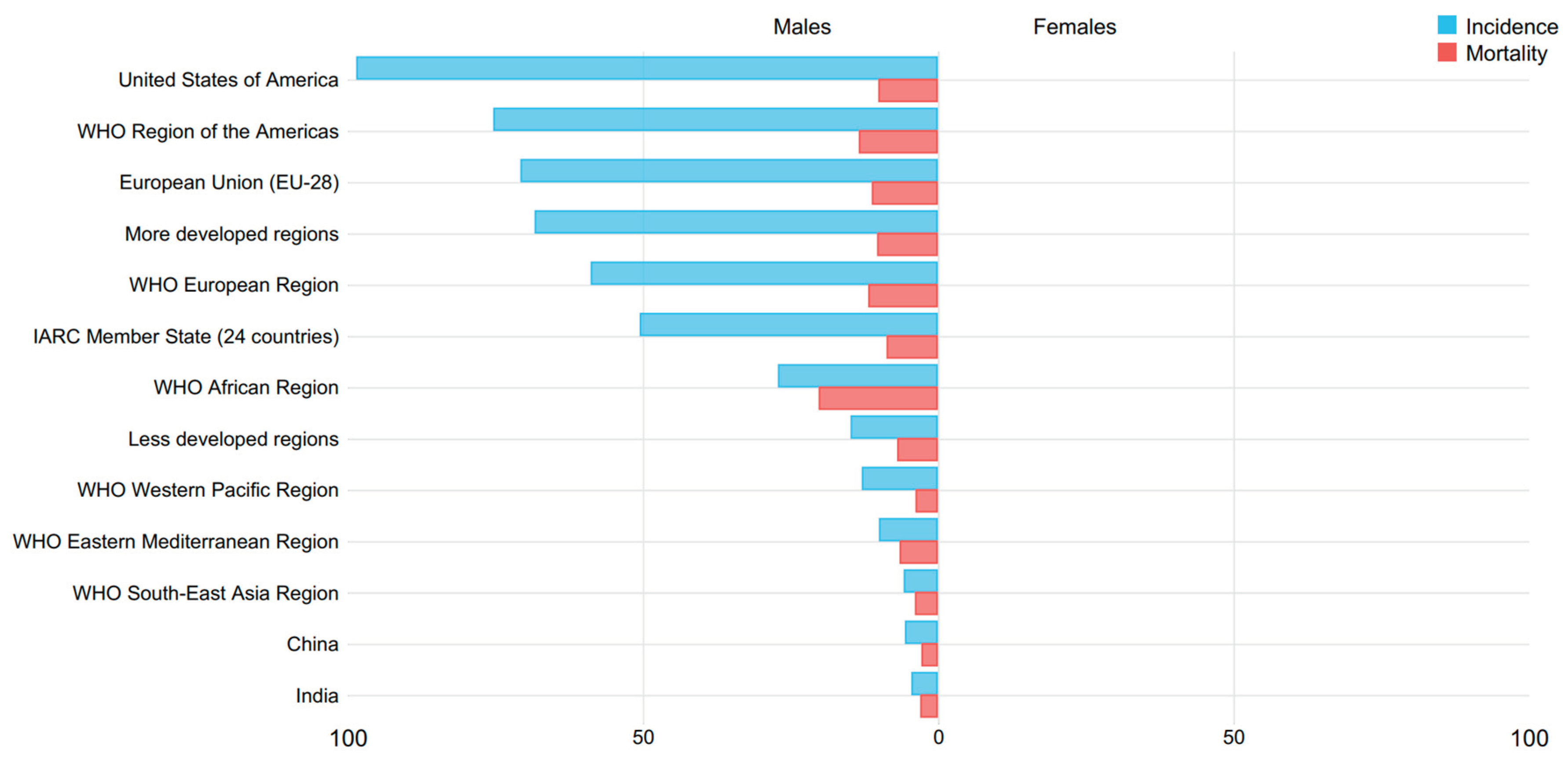
Table 2.1. Estimated incidence and mortality worldwide in 2012.

Table 2.1. Estimated incidence and mortality worldwide in 2012.

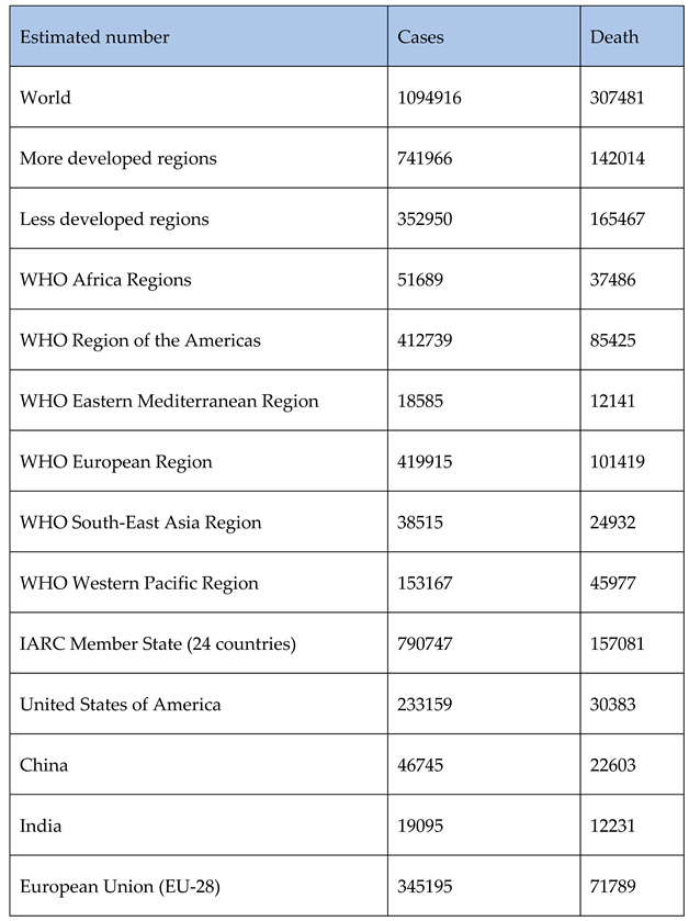Figure 2.2. Estimated age-standardized rates (World) of incidence cases, males, prostate cancer geographical mapping, worldwide in 2012.

Figure 2.2. Estimated age-standardized rates (World) of incidence cases, males, prostate cancer geographical mapping, worldwide in 2012.

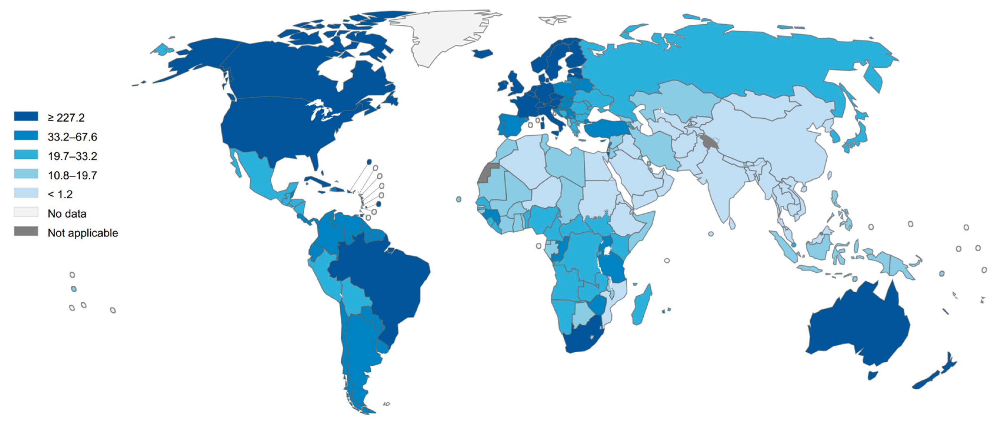
Figure 2.3. Estimated age-standardized rates (World) of incidence cases, males, prostate cancer trend, worldwide in 2012.

Figure 2.3. Estimated age-standardized rates (World) of incidence cases, males, prostate cancer trend, worldwide in 2012.

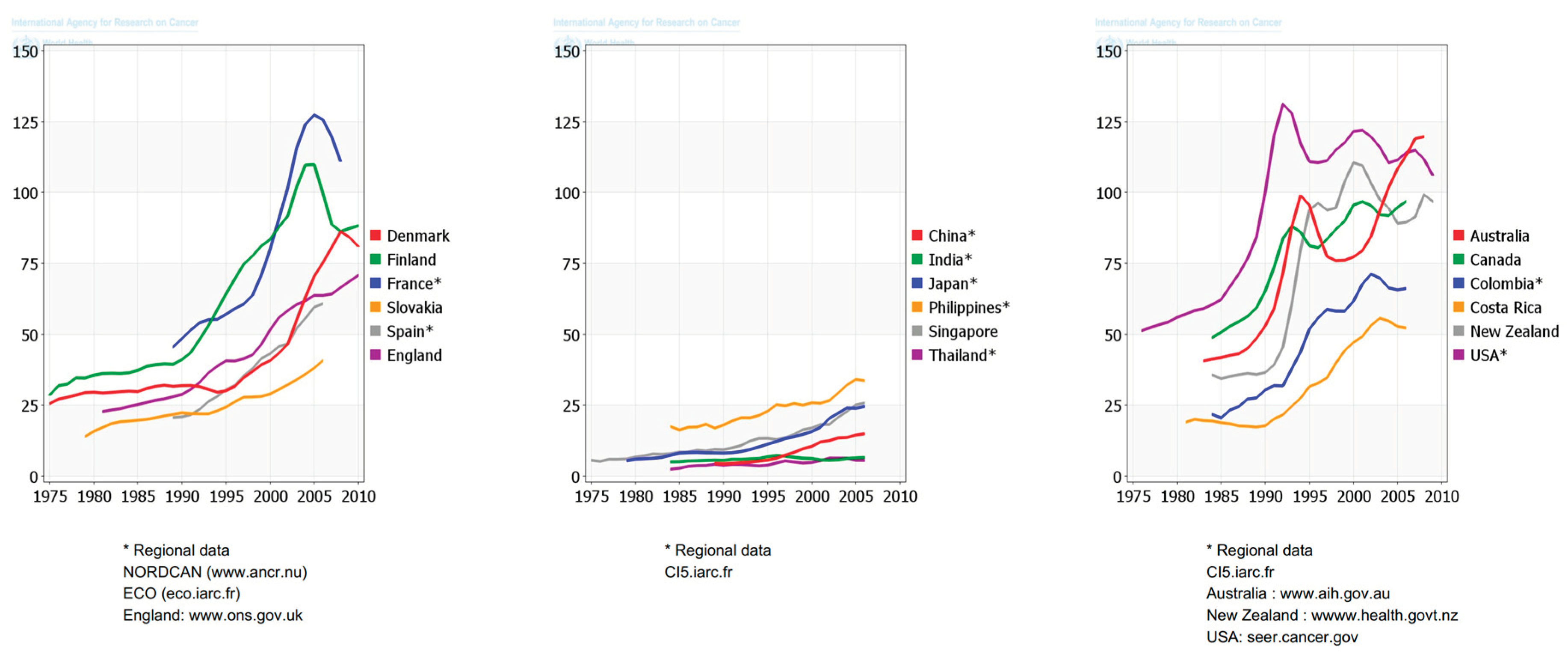
Figure 2.4. Estimated age-standardized rates (World) of deaths, males, prostate cancer geographical mapping, worldwide in 2012.

Figure 2.4. Estimated age-standardized rates (World) of deaths, males, prostate cancer geographical mapping, worldwide in 2012.

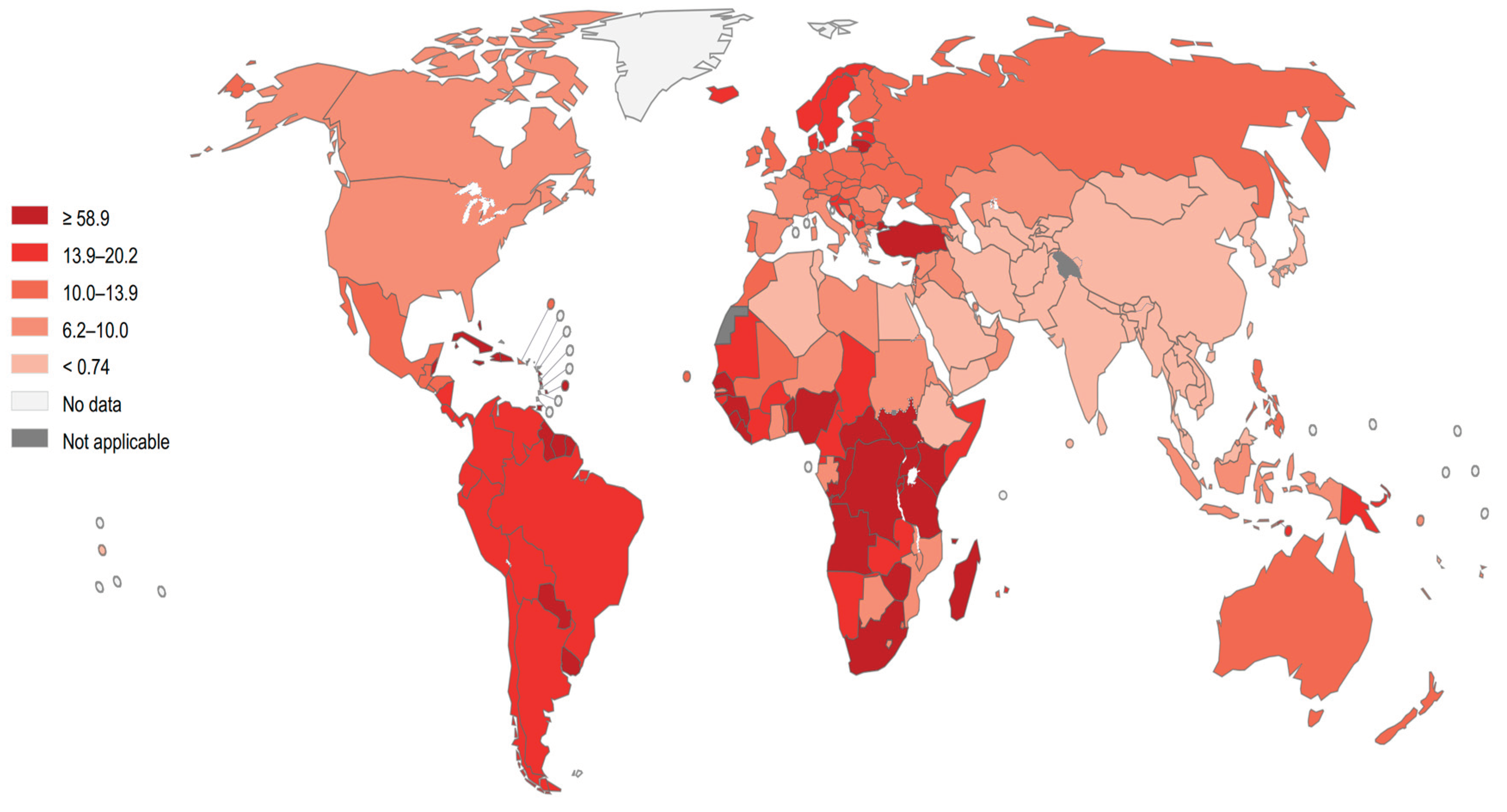
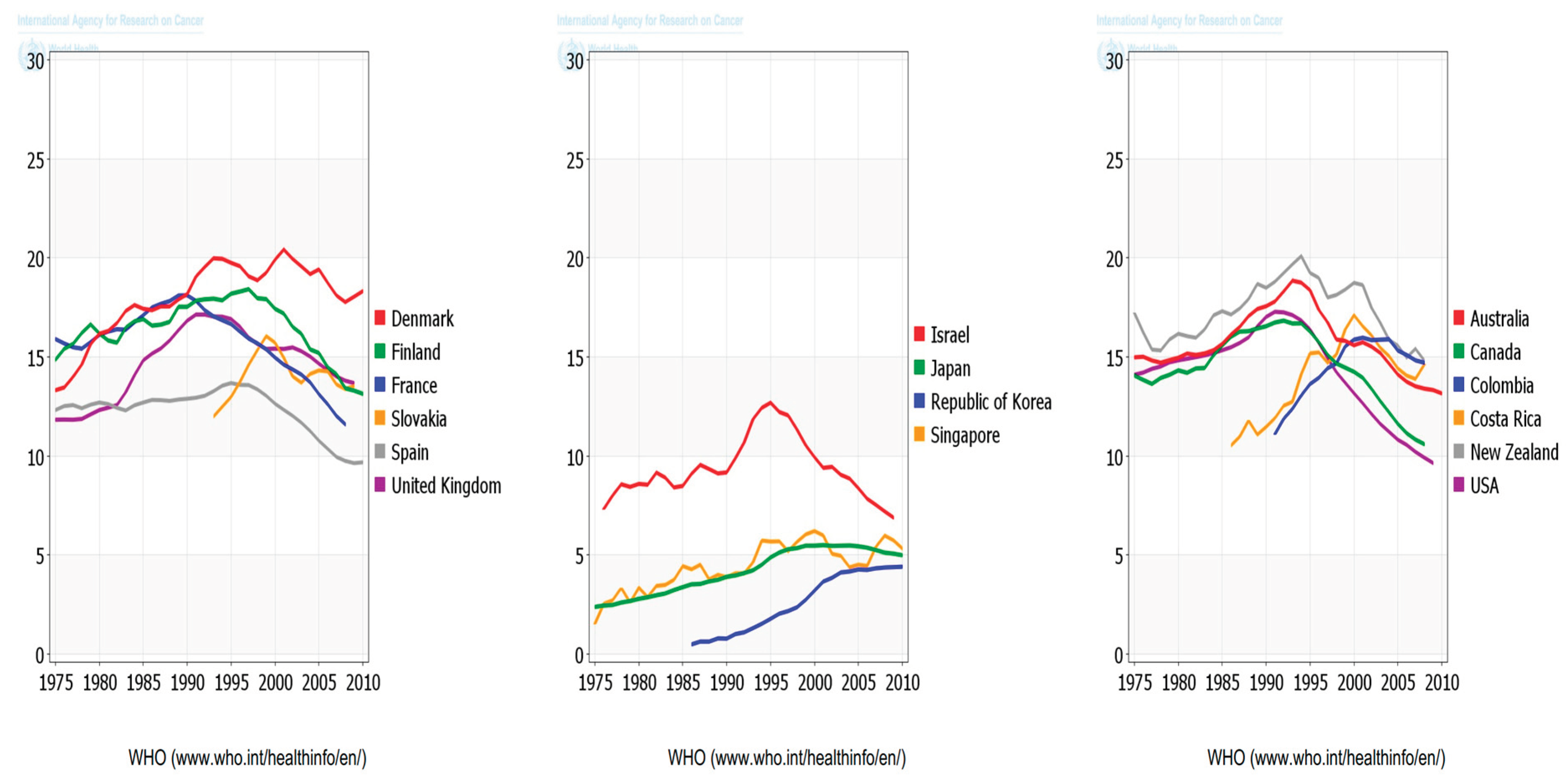
Figure 2.5. Estimated age-standardized rates (World) of incidence cases, males, prostate cancer trend, worldwide in 2012.

Figure 2.5. Estimated age-standardized rates (World) of incidence cases, males, prostate cancer trend, worldwide in 2012.

According to the World Health Organization (WHO), Cancer is the second leading reason for death globally, accounting for 9.6 million deaths estimation, (or one in six deaths). Lung, prostate (1.28 million cases), colorectal, stomach and liver cancer are the commonest types of cancer in men, whereas breast, colorectal, lung, cervical and thyroid cancer are the commonest among ladies (WHO, 2018).

Figure 2.6. Number of new cases (a) and deaths (b) in 2018, both sexes, all ages.

Figure 2.6. Number of new cases (a) and deaths (b) in 2018, both sexes, all ages.

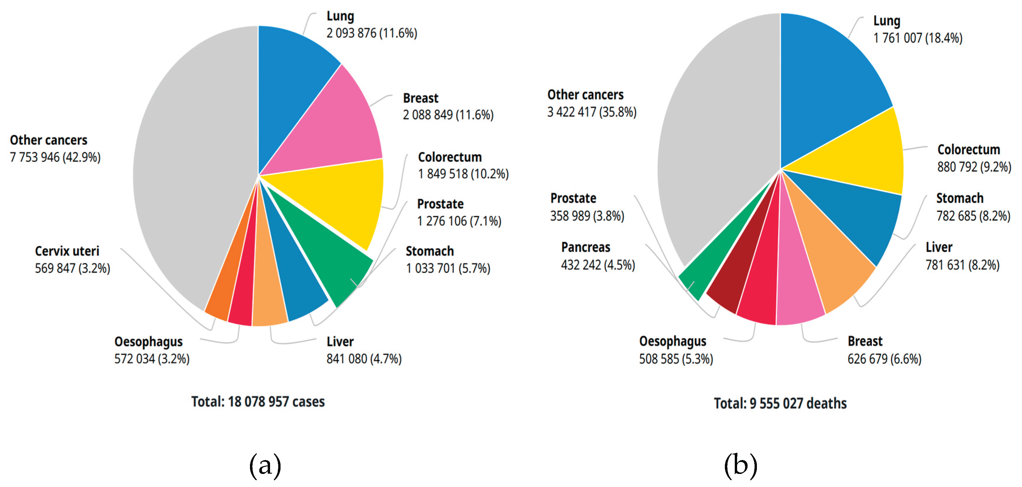
Table 2.2. Cancer incidence and mortality statistics worldwide and by region.

Table 2.2. Cancer incidence and mortality statistics worldwide and by region.

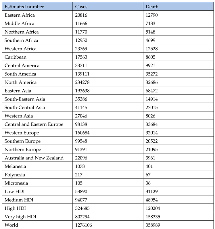Figure 2.7. Incidence (a) and Mortality (b), both sexes.

Figure 2.7. Incidence (a) and Mortality (b), both sexes.

Figure 2.8. Age-standardized (World) incidence rates, prostate, all ages.

Figure 2.8. Age-standardized (World) incidence rates, prostate, all ages.

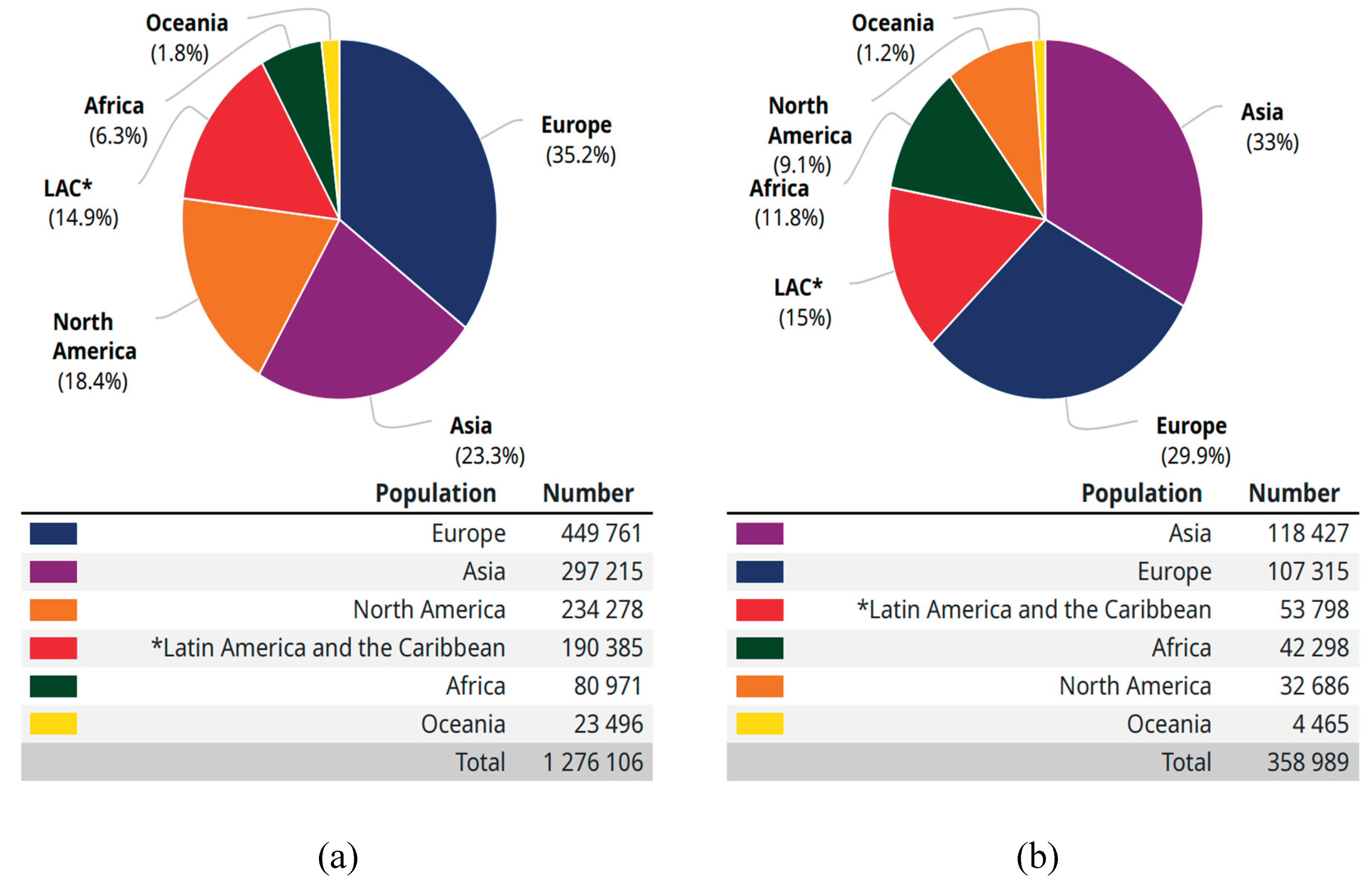
Figure 2.9. Age-standardized (World) mortality rates, prostate, all ages.

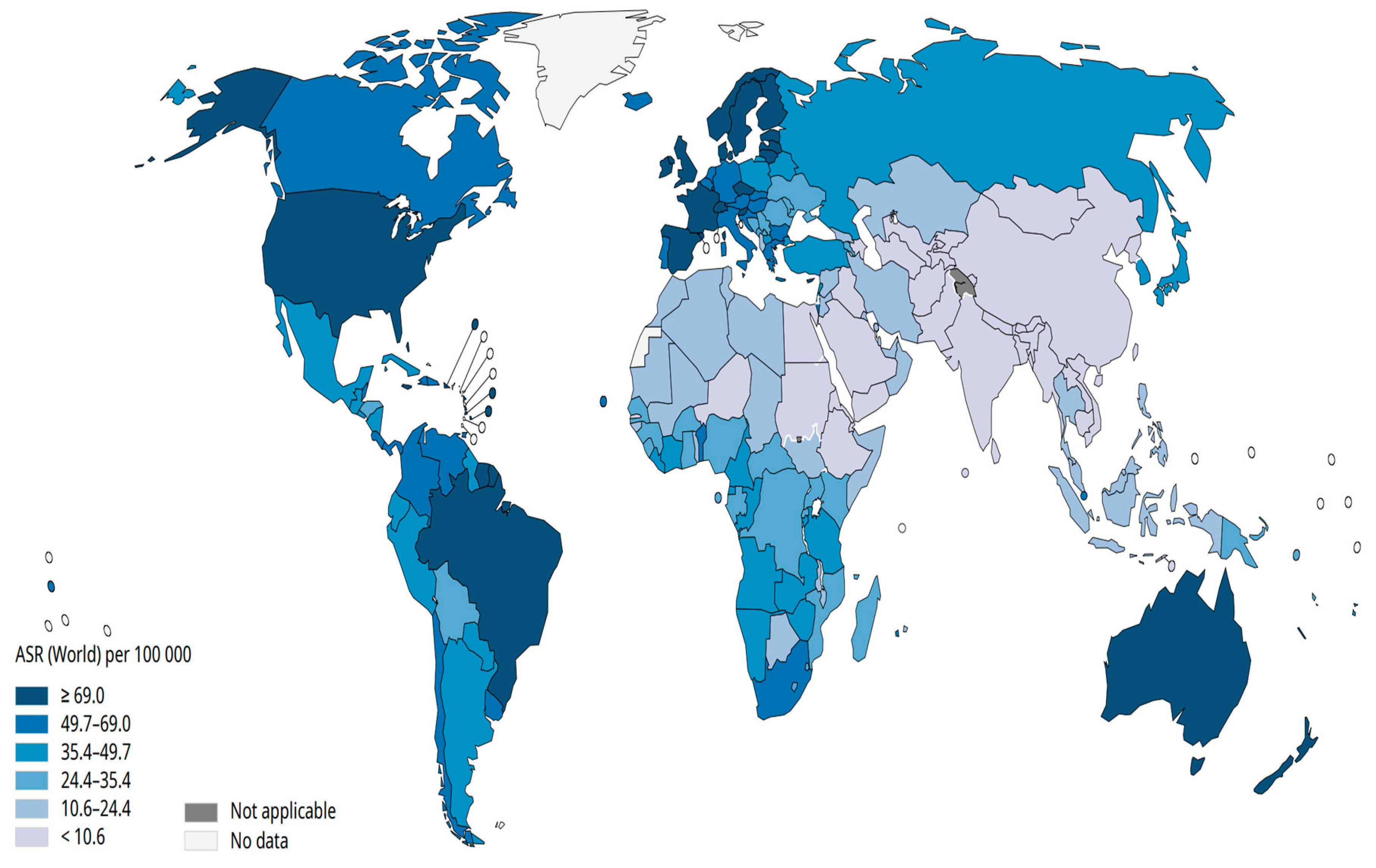
Figure 2.9. Age-standardized (World) mortality rates, prostate, all ages.

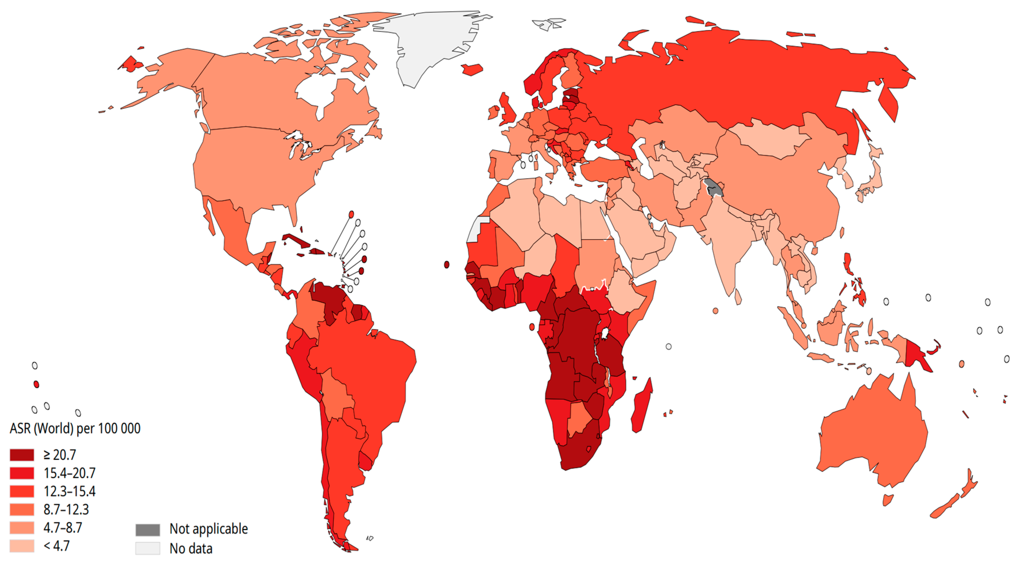
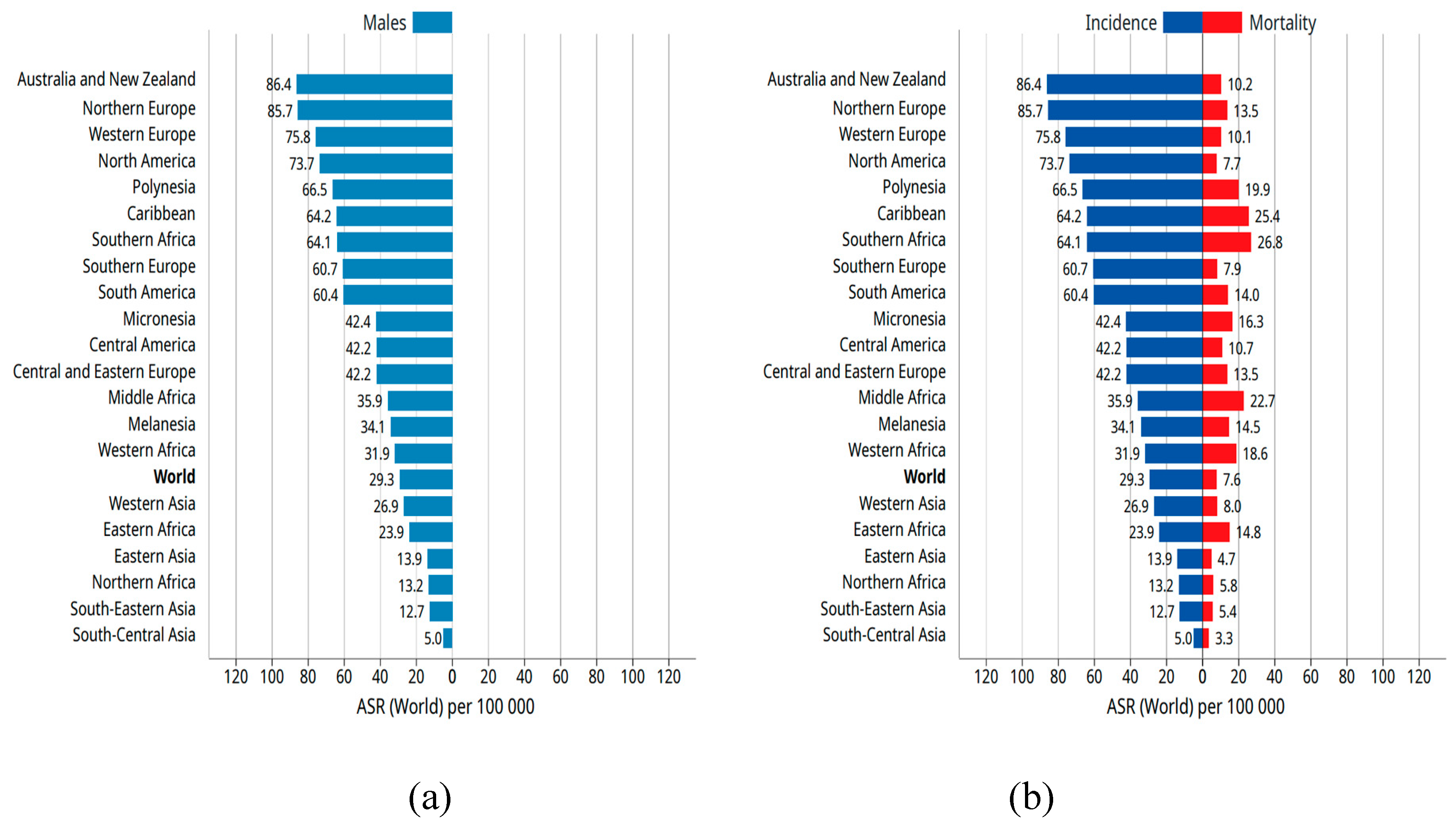
Figure 2.10. Age-standardized (World) incidence rates, prostate, by sex (a) and Age-standardized (World) incidence and mortality rates, prostate.

Figure 2.10. Age-standardized (World) incidence rates, prostate, by sex (a) and Age-standardized (World) incidence and mortality rates, prostate.

Prostate cancer is cancer that happens within the prostate — a little walnut-shaped secreter (gland) in men that produces the seminal fluid that nourishes and transports spermatozoon. it's one amongst the foremost common forms of cancer in men. Prostate cancer usually grows slowly and is initially constricted to the prostate secreter, where it should not cause serious harm or damages. However, while some kinds of prostate cancer growth rate are slow and may need minimal or even no treatment, other kinds are aggressive and can unfold rapidly. Prostate cancer begins once some cells in your prostate become abnormal. Mutations within the abnormal cells' deoxyribonucleic acid cause the cells to grow and divide sooner than healthy cells do. The abnormal (unhealthy) cells continue living while other cells would die. The accumulating abnormal cells form a tumor which then grows to invade near tissue. Some abnormal cells also can break off and unfold (metastasize) to different organs of the body. While several factors can increase the risk of prostate cancer, research and analysis has highlighted age, race, family history and fatness as the major factors to prostate cancer (Prostate Cancer - Symptoms and Causes - Mayo Clinic, n.d.).

2.2. Prostate metastasis severity detection

There is a scarceness of high-level proof that early that early diagnosis of prostate cancer can forestall or minimize the issues ensuing from an outsized girdle tumor however one in all the foremost contentious topics in medication continues to be whether or not testing for this quite common tumor is within the best interests of individual patients. though there's a spectrum of progression rates for this tumor, in most instances, prostate cancer replicates and spreads slowly. As this tumour is uncommonly diagnosed before the age of forty years and therefore the chance of clinical detection will increase as men age, most patients have comorbidities once diagnosed with glandular (prostate) cancer. For this reason and since there aren't insignificant potential disadvantages with the detection method and its consequences, it's necessary to see whether or not the advantages of detection are likely to be greater than the unwanted effects of leaving a possible prostate cancer undiagnosed. (Roberts et al., 2000). Several methods exist for detecting prostate metastasis. Most prostate cancers are first found as a result of screening with a prostate-specific antigen (PSA) blood test or a digital rectal exam (DRE).

2.2.1.1. Prostate-specific antigen (PSA) blood test

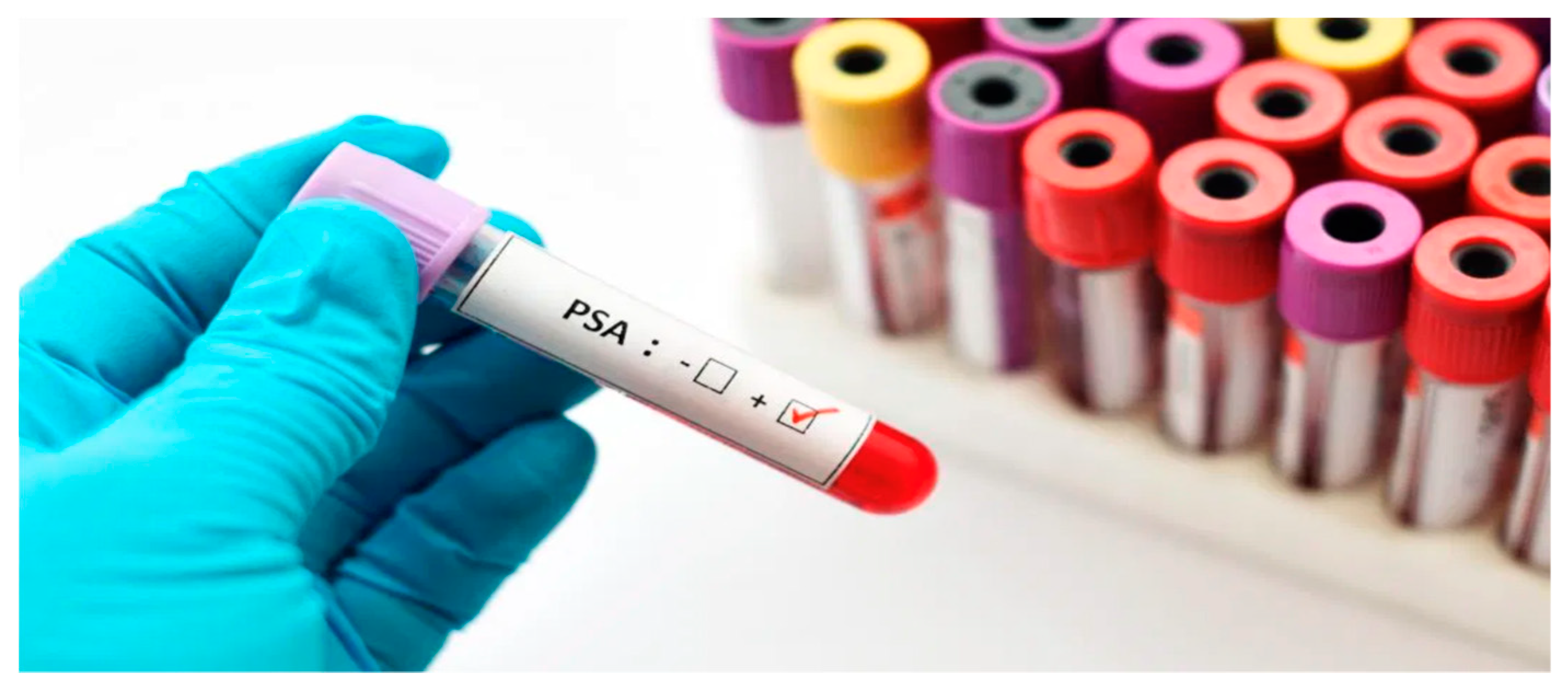
Prostate-specific antigen (PSA) is a protein made by cells within the ductless gland (both normal cells and cancer cells). PSA is usually found in body fluid (Siemen), however a tiny low quantity is additionally found within the blood. The PSA level in blood is measured in units referred to as nanograms per cubic centimeter or milliliter (ng/mL). The prospect of having prostate cancer goes up as the PSA level goes up, however no set cutoff point can tell for sure if a man has prostate cancer or not. several doctors use a prostate specific antigen cutoff point of 4 ng/mL or higher when deciding if a man might need further testing, whereas others may advocate it beginning at a lower level, such as 2.5 or 3. One reason it’s onerous to use a set cutoff point with the prostate specific antigen test when searching for prostate cancer is that many factors aside from cancer may have an effect on PSA levels. Factors like age enlarged prostate, redness, ejaculation, riding a bicycle, sure medical specialty such as urology procedures, certain medicines and medications, 5-alpha reductase inhibitors, herbal mixtures etc. could alter (raise or lower) PSA levels

Figure 2.11. PSA test (Free PSA: Test, Results, and Prostate Cancer, n.d.).

Figure 2.11. PSA test (Free PSA: Test, Results, and Prostate Cancer, n.d.).

2.2.1.2. Digital rectal exam (DRE)

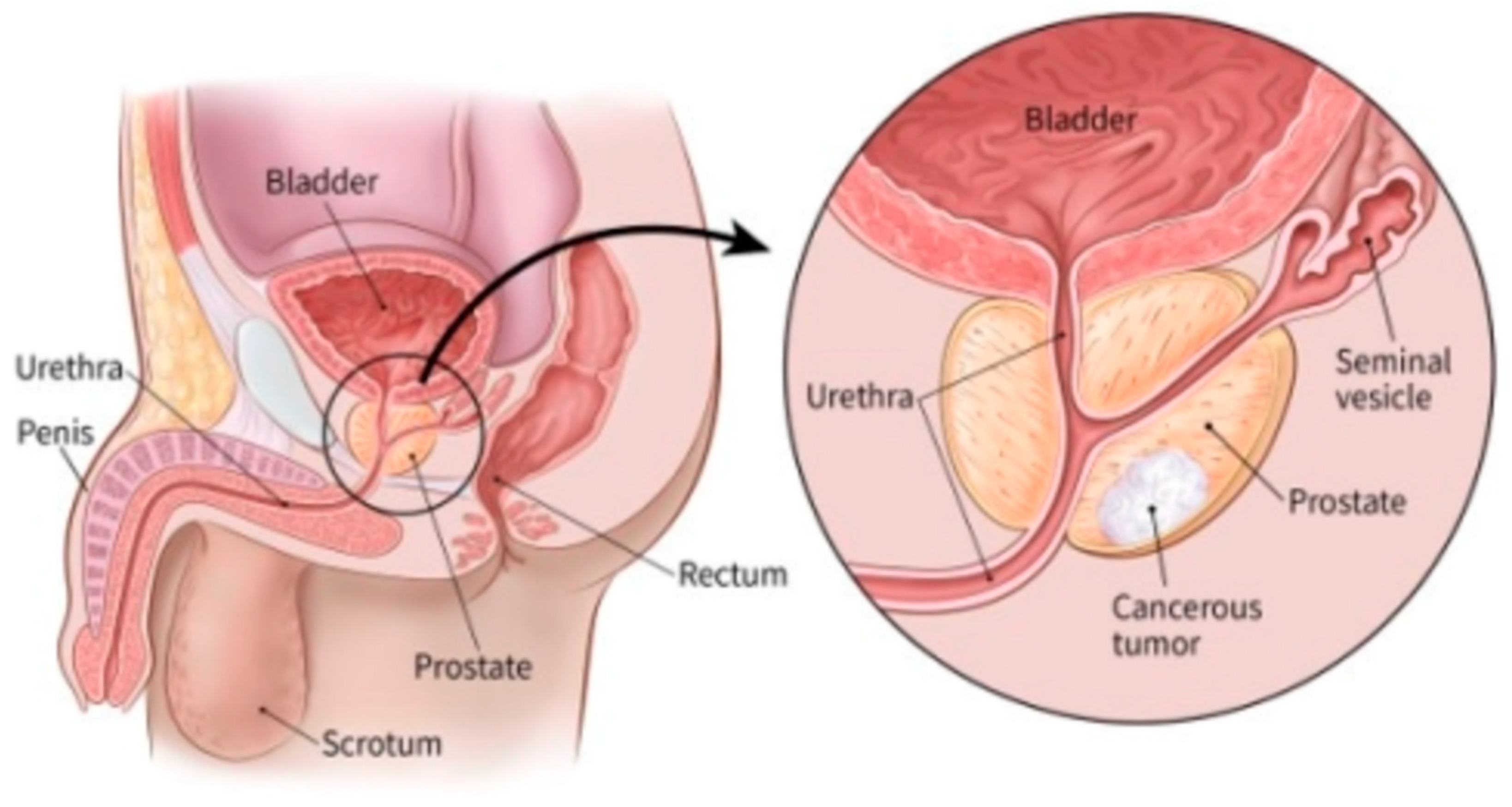
For a digital rectal examination (DRE), the doctor inserts a gloved, lubricated finger into the body part (rectum) to feel and gently check for any bumps or exhausting areas on the prostate that may be cancer. Prostate cancers many times begin within the back a part of the gland and may typically be felt when performing a rectal test. This test is often uncomfortable (especially for who have hemorrhoids), however it always isn’t painful and solely takes a brief time. DRE is less effective than the PSA biopsy at finding prostate cancer, however it can sometimes find cancers in men with normal PSA levels.

Figure 2.12. Detect prostate cancerous tumor with DRE.

Figure 2.12. Detect prostate cancerous tumor with DRE.

2.2.2. Biopsy methods for Prostate Cancer

The screening tests mentioned above (PSA biopsy, DRE, or other tests) are used to look for possible signs of prostate cancer. however, these tests can’t tell as expected if you have got cancer. If the results of one among these tests is abnormal, there'll in all probability be a necessity for prostate diagnostic test (biopsy) to know for sure if you have got cancer.

A biopsy is a procedure during which little samples of the prostate are removed then checked out with a magnifier or microscope. A core needle biopsy is the main method used to diagnose prostate cancer and it's mostly carried out by a specialist (urologist) to determine the presence, cause and extent of disease in a living body. in line with (Brunese et al., 2020), biopsy for prostate cancer can be done in several ways which can generally be categorized into:

• The invasive methods: These are medical procedures that invade the body usually by puncturing or cutting the skin or by inserting medical instruments into the body. According to (Thomas, n.d.), the 3 major techniques used within the invasive methodology are:

  (a)

  transrectal ultrasound (TRUS) guided systematics biopsy: This is considered to be the best among these methods. The procedure is usually done after sedation whereby a doctor inserts an ultrasound probe into the rectum to obtain images of the prostate.

  (b)

  transurethral biopsy: this methodology is not usually employed and involves the insertion of cystoscope into the urethra with the aim of recovering tissue samples from the prostate through the urethral wall.

  (c)

  transperineally prostate biopsy: this method is becoming popular due to the better opportunity it offers at sampling the prostate in a systematic manner whereby, a brachytherapy template is used to recover tissue for examination.

• The non-invasive methods: These are medical procedures in which there is no break in the skin. In prostate cancer imaging, the magnetic resonance imaging (MRI) with ultrasound are being introduced to achieve targeted prostate biopsy instead of blind systematic biopsies. The techniques have been proven to be the best currently due to the level of accuracy and high detection rate in diagnosis.

The end goal of any of these biopsies is to get the current representation of the cells which can then be further examined for prostate metastasis grading. Gleason score or grade can be calculated using different techniques and approaches based on the method of choice.

2.2.3. Gleason Score

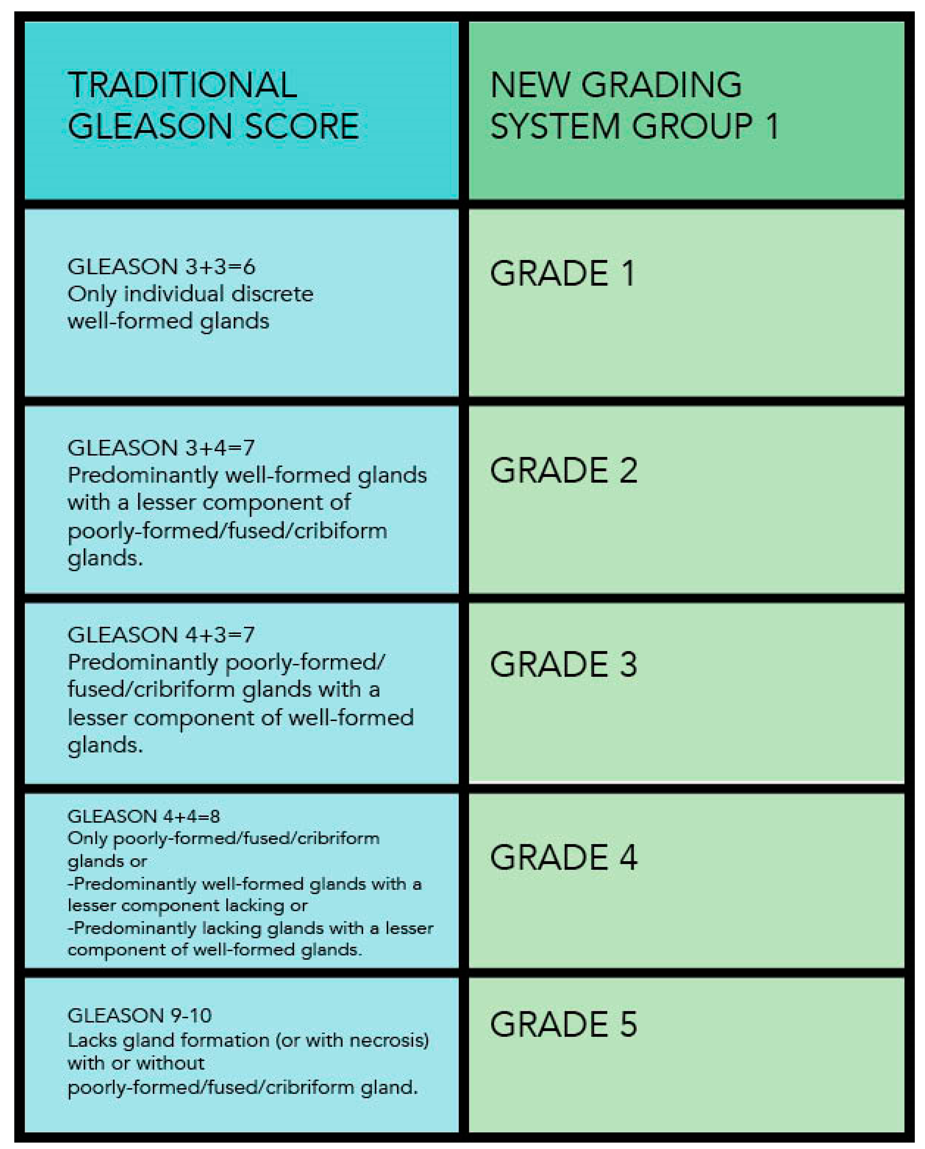
The strongest correlating predictor of recurrence for prostate cancer is the Gleason score is the but has substantial inter-observer variability, limiting its usefulness for individual patients. Specialized urological pathologists do have a greater concordance, but such expertise and experience are not widely available and accessible. Therefore, prostate cancer diagnostics could benefit from reproducible, robust Gleason grading. Gleason score is a grading system used in the determination of the severity or aggressiveness of diagnosed prostate cancer. Donald Gleason, a pathologist devised this grading system that ranges between 1 (low risk) and 5 (high risk) to explain the severity of cancerous cells from a biopsy. According to Gleason, cancerous cells can be grouped into five different patterns based on the changes that can occur in normal cells to tumorous cells. lower grade tumor cells are those with a score of 1 or 2 while higher-grade tumor cells are those closer to a score of 5. The lower graded cells usually look similar to healthy cells and the higher graded cells look entirely different from a regular cell due to mutation. The Gleason score in biopsies is the sum of the most common pattern (primary) and the highest secondary pattern (e.g. 3+5). In the latest revision of the Gleason grading system, five prognostically distinct grade groups were introduced; assigning scores 3 + 3 and lower to group 1, 3 + 4 to group 2, 4+3 to group 3, 3+5, 5+3, and 4+4 to group 4, and higher scores to group 5. Although clinically relevant, initial research shows that this transition has not reduced the observer variability of the grading system, (Ryu et al., 2019).

Figure 2.13. Demystified Gleason scores and meanings.

Figure 2.13. Demystified Gleason scores and meanings.

2.2.3.1. Methods and Approaches to Gleason Score Prediction

After a biopsy has been carried out, the resulting images need further examination for grading to measure the severity of the prostate cancer which is key in determining in identifying appropriate, patient-tailored treatment options. Several methods and techniques have been proposed, experimented with and used in the determination/prediction of Gleason Score.

A review by (Vargas, 2014) to determine prostate cancer aggressiveness via Gleason scoring system, Whole-Lesion Histogram Analysis of the Apparent Diffusion Coefficient was used. This method intends to evaluate the relationship between prostate cancer aggressiveness and histogram-derived apparent diffusion coefficient (ADC) parameters obtained from Whole-Lesion assessment of diffusion-weighted magnetic resonance (MR) metric to The ADC may be a comparatively easy metric which will be calculated on a pixel-by-pixel basis with the quality clinical commercial magnetic resonance imaging platforms after which the mean or media can be used to correlate the ADC values with the prostate cancer Gleason scores. However, there is no consensus on the best metric to determine lesion ADCs derived from the multiple pixels that are contained within each prostate cancer focus. The standardization of quantitative ADC metrics is of crucial importance in order to establish the ADC as a robust and sturdy biomarker for predicting prostate cancer Gleason scores. The heterogeneous nature of prostate cancer imposes bound limitations on a number of the most commonly used metrics. In contrast to the traditional practice of treating medical images as pictures intended solely for visual interpretation, the emergence of radionics which is a method used in the extraction of a large number of features from radiographic medical images using data characterization algorithms opened lots of possibilities at the application other advance techniques in the determination and prediction of the Gleason score with improved and better predictive accuracy.

In accordance to (Brunese et al., 2020), a set of radiomic biomarkers can be computed directly from magnetic resonance image making it possible to obtain high-quality medical radiomic featured images using the non-invasive approach. In his contribution, he provided a formal model fully based on an algorithm designed by him to detect the prostate cancer Gleason score and whether the prostate cancer needs surgical treatment. the formal specifications considered for the formal model heavily on mathematical syntax and semantics. The system behavior was represented with as Labeled transition System (LTS) consisting of a set of nodes and a set of a labelled edge connecting the nodes. With this model, one can detect the Gleason score and the surgery treatment is predicted directly from MRIs exploiting radiomic features. Though this formal method can discriminate between several Gleason scores prostate cancers and even predict the surgery treatment, but there is no room for improvement without altering the entire system designed. The use of radiomic features as a non-invasive biomarker in the prediction of the Gleason score for prostate cancer never seized as seen in (Chaddad et al., 2018). Studies emphasized on the fact that prostate-specific Antigen alone is not an accurate indicator of prostate cancer but rather, the combination with magnetic resonance (MR) imagery of the type multi-parametric sequence can contribute greatly in diagnosis, staging and treatment monitoring of different types of tumor. In addition to this, Prostate Imaging Reporting and Data System showed that this scoring method is capable of predicting the risk of prostate cancer presence based on the MR images. However, the method is highly dependent on the interpretation of the images from the experienced radiologists that carried out inter-reader variability. Non-invasive techniques for the analysis of tumor properties based on MR images known as radiomics has recently been the starting point for tumor heterogeneity study to properly determine the associated Gleason score. Leveraging machine learning on radiomic features has made it possible to analyze large numbers of prostate cancer images which is gradually eradicating the limitations to Gleason score prediction.

2.3. Artificial Intelligence in Gleason score grading system

Artificial intelligence like machine learning and notably deep learning has the potential to improve the standard and quality of Gleason grading by improving consistency and providing expert-level grading independent of location (Ryu et al., 2019). The use of machine learning and deep learning in the determination of prostate cancer aggression through Gleason score prediction cannot be neglected. Trained models may be used to automate pattern identification utilized in decision-making and extract predictions on future data (Lee et al., 2017).

2.3.1. Machine learning for Gleason score prediction

Machine learning, a branch of artificial intelligence which uses a variety of probabilistic, statistical and optimization techniques that allows computers to learn and detect latent patterns from past examples in large, noisy and complex data sets has greatly been used in Gleason score prediction. As seen in (Cruz & Wishart, 2006), Early use of machine learning in cancer research centered around identifying, classifying, detecting, or distinguishing tumors and other malignancies. In different words, ML has been used primarily as an aid to cancer detection and diagnosing. But of recent, researchers have tried to use machine learning for cancer prediction and prognosis. There are many machine learning algorithms readily available for researchers depending on the method of approach and dataset. These algorithms can majorly be categorized into unsupervised, supervised and reinforcement learning. Most researches that have adopted artificial intelligence in Gleason score prediction utilizes supervised learning which is a type of machine learning that learns from historical labelled data. (Citak-Er et al., 2014) used discriminant analysis and Support Vector Machine to predict Gleason score based on Preoperative Multiparametric MR imaging of Prostate Cancer. Computer-aided detection and diagnosis (CAD), which is a combination of imaging feature engineering and ML classification, has shown potential in assisting radiologists for accurate diagnosis, decreasing the diagnosis time and the cost of diagnosis. Traditional feature engineering methods are based on extracting quantitative imaging features such as texture, shape, volume, intensity, and various statistical features from imaging data followed by an ML classifier such as Support Vector Machines (SVM), Adaboost, and Decision Trees etc. (Yoo et al., 2019). Several studies have shown the diagnostic power of multiparametric MRI for prostate cancer. In their study, a computer-aided diagnosis system that combined clinical and multiparametric MR findings were developed to predict preoperatively the final Gleason score of prostate cancers. While various machine learning algorithms were tested for the prediction and classification of prostate cancer and they mainly differed in the selection of the predictive parameters, the 5-point Likert scales of prostate MR images have not been previously evaluated. Linear discriminant analysis and support vector machine (SVM) classifiers which is a type of supervised machine learning algorithm were compared for their classification performances after a standard or a Gaussian kernel principal component analysis. Additionally, the work evaluated the contributions of the predictive parameters on prostate cancer malignancy detection by employing an SVM based recursive feature elimination and utilized the kernel trick to enhance the performance of classifiers. The SVM algorithm performed better at the construction of optimal separating hyperplane that maximizes the margin where the margin is the largest distance to the nearest training data point of any class. A major success was recorded when MRI along with prostate cancer analysis was used in the research. While magnetic resonance imaging has been rumored to own diagnostic worth for prostate cancer, it was proposed that quantitative diffusion tensor imaging (DTI) analysis can be used to discriminate PC from normal tissue. The application of a Gaussian kernel PCA improved the performances of each classification models for an accurate prediction of final Gleason score based on clinical findings and preoperative multiparametric Magnetic Resonance imaging for the limited patient population whereas exploiting the complicated relationship between predictive features. The LDA provided gave marginally higher clearness than the SVM strategy, which might be known with the tiny intraclass separation. It was seen that multiparametric-MRI highlights were a higher priority than clinical highlights dependent on SVM-RFE scores, and applying highlight disposal technique expanded the order exhibitions of the models.

2.3.2. Deep learning for Gleason score prediction

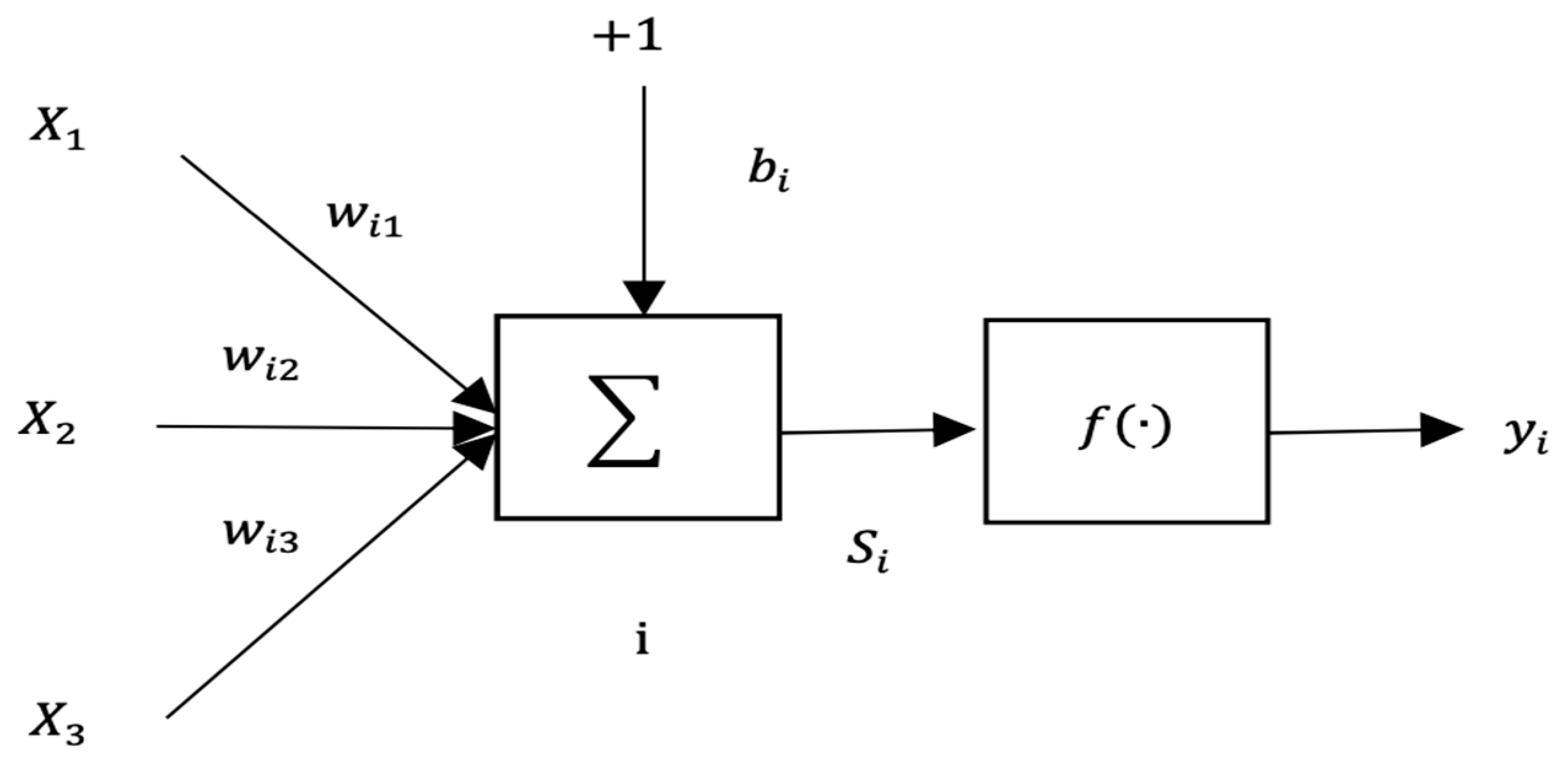
Deep learning is a form of machine learning which aims to mimic functions of the biological human brain by making use of a multi-layered neural network which allows the transfer of information, through interconnected layers, for analysis and decision-making (Lee et al., 2017). Deep learning has already been investigated and shown promising use in diagnostics in several medical fields with examples in radiology, ophthalmology, dermatology, and pathology (Ryu et al., 2019) due to its outstanding performance in computer vision tasks such as segmentation, classification, and object detection. Previous studies have applied feature-engineering (a very useful tool in machine learning) approaches to address Gleason grading. Eventually, the field transitioned to deep learning application in detecting cancer. An artificial neural network (ANN) consists of multiple neurons.

Figure 2.14. The structure diagram of a neuron (Y. Liu & An, 2018).

Figure 2.14. The structure diagram of a neuron (Y. Liu & An, 2018).

Deep Learning methods consist of convolution layers that can extract different features from low-level local features to high-level global features from input images. A fully connected layer (ANN) at the end of the convolutional neural layers (CNN) converts convoluted features into the probabilities of certain labels. A simple structure diagram of CNN is shown in the figure below

Figure 2.15. The structure diagram of CNN (Y. Liu & An, 2018).

Figure 2.15. The structure diagram of CNN (Y. Liu & An, 2018).

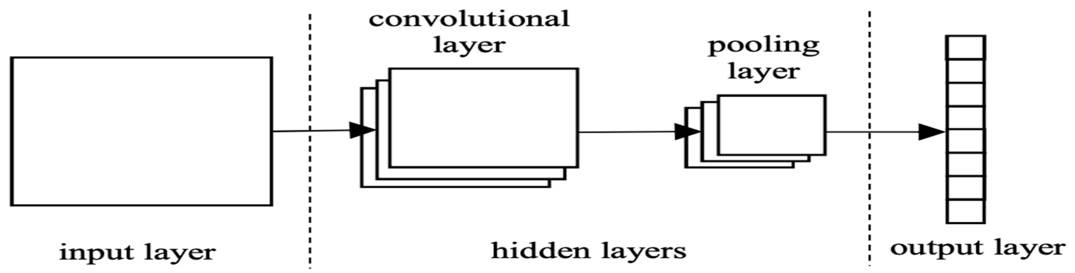
Different types of layers, such as batch normalization layer, which normalizes the input of a layer with a zero mean and a unit variant, and dropout layer, which is one of the regularization techniques that ignores randomly selected nodes, have been shown to improve the performance of deep learning-based methods. The layered structure of a CNN is therefore what allows the extraction of features that are so complex or subtle that they may be unknown or not easily identifiable by humans. Nevertheless, to achieve convincing performance, optimal combinations and structures of the layers, precise fine-tuning of hyper-parameters as well as computational resources are required. This remains as one of the main challenges of deep learning-based methods when applied to different fields such as medical imaging (Yoo et al., 2019). There several varieties of deep learning architectures for image analysis based on the desired end goal and layers are arranged to meet needs. This flexibility has given room for researcher and deep learning practitioners to implements lots of state-of-the-art architecture of which CNN finds itself most useful in almost all.

U-Net is an example of convolutional neural network architecture optimized for image segmentation. It consists of an encoder and decoder pathway with skip connections that allow recovery of the original image resolution while providing voxel-based segmentation into tissue classes. There are several others of which some has been named based on the level of hidden layer in them while others are named based on the structure of the architecture.

Figure 2.16. The architecture of the U-Net based network. Each blue box denotes the feature map with multi-channels (Zhang et al., n.d.).

Figure 2.16. The architecture of the U-Net based network. Each blue box denotes the feature map with multi-channels (Zhang et al., n.d.).

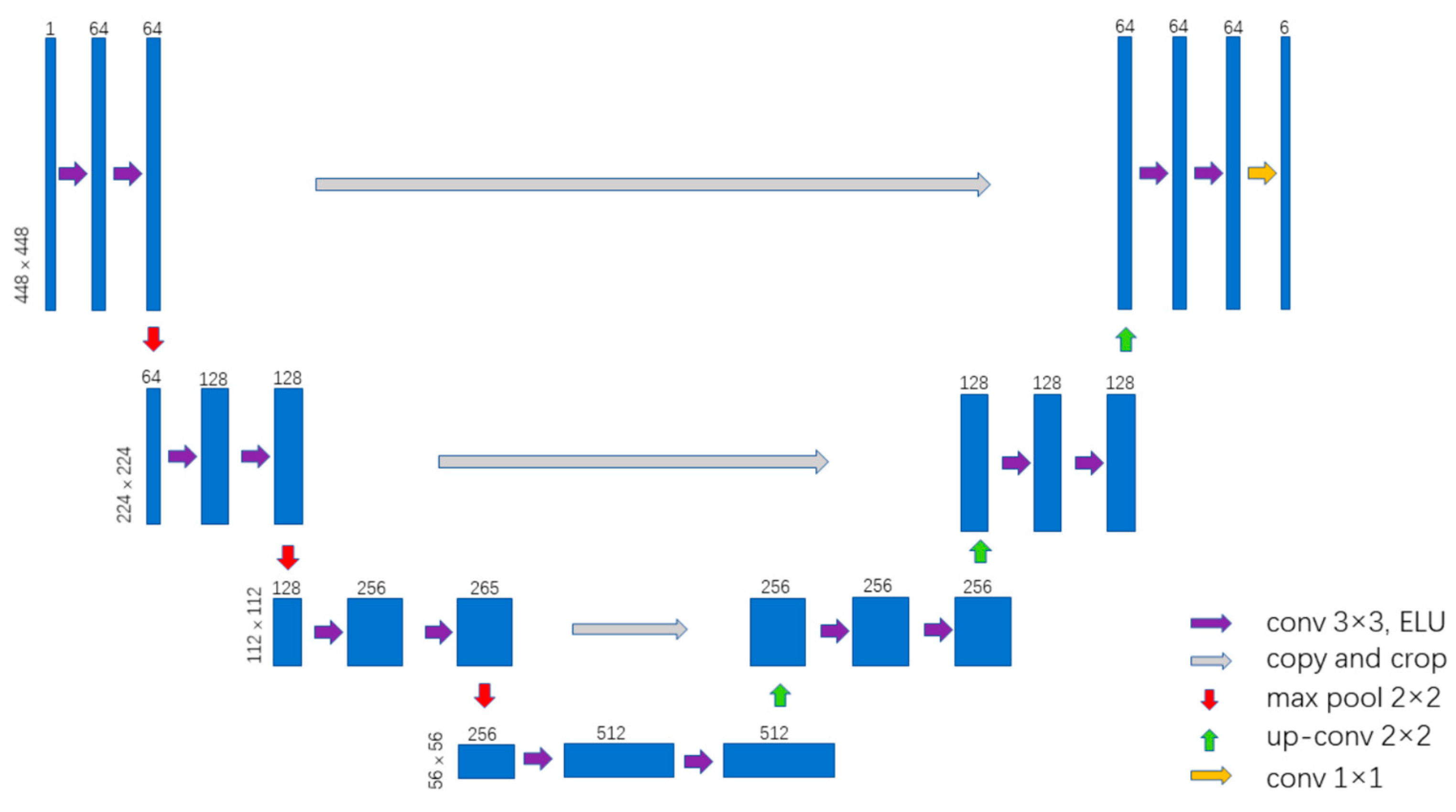
Another good example of CNN architecture is the XmasNet inspired by VGG net which performed greatly on the dataset it was trained on (S. Liu et al., 2017). XmasNet architecture is described in the figure below.

Figure 2.17. The architecture of the XmasNet. Conv: convolutional layer; BN: batch normalization layer; ReLU: rectified linear unit; Pooling: max-pooling layer; FC: fully connected layer.

Figure 2.17. The architecture of the XmasNet. Conv: convolutional layer; BN: batch normalization layer; ReLU: rectified linear unit; Pooling: max-pooling layer; FC: fully connected layer.

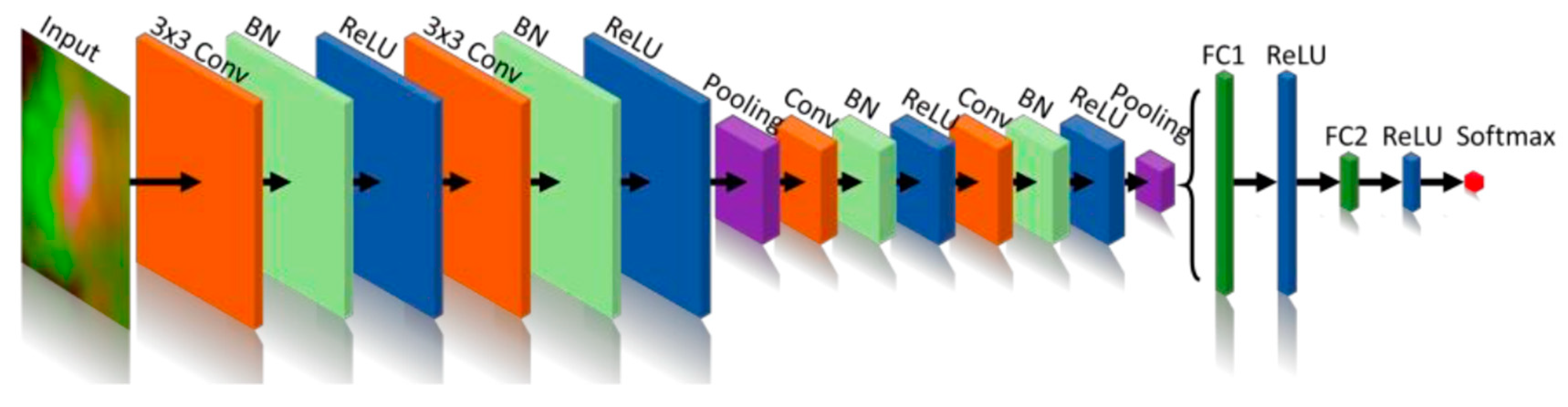
The list of these architectures is endless as there are countless ways the different components of CNN architecture can be arranged. The main limitation of deep learning, which has significance for medical applications, is the high dependency on large amounts of high-quality data (Lee et al., 2017). The reason for the lack of large medical image data sets is that medical images are often costly to acquire, and a large amount of work needs to be done by experts to produce and label the images. Furthermore, there are privacy and ethical issues with collecting and analyzing medical images which need to be overcome to ensure that patient integrity are not breached (Lakhani et al., 2018). To overcome the problem of insufficient data sets, the most common and effective methods are data augmentation, transfer learning or the use of generative models such as generative adversarial networks (GANs).

2.3.2.1. Data Augmentation

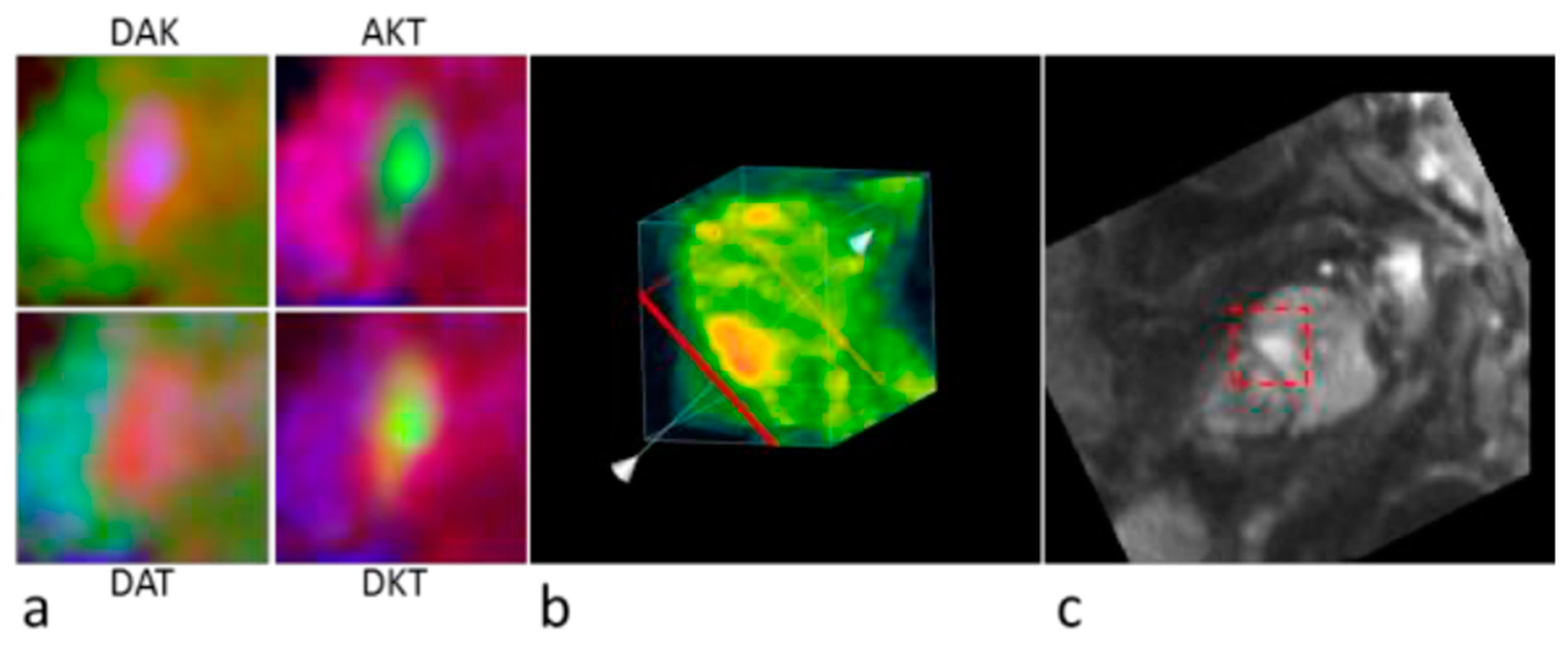
A common problem encountered when training a deep learning model on a limited dataset is memorization which occurs when the model becomes too closely fitted to the training data (Wong et al., 2016). For example, instead of grouping medical image data into “affected” and “unaffected”, for a particular disease, an inadequately trained deep learning algorithm would correctly classify the training image dataset and any new image (affected or un-affected) as un-affected as it is not part of the original affected training group. To prevent overfitting or memorization of the training data and increase the accuracy and generalization of CNNs, the training data can be augmented (Wong et al., 2016). Traditional methods of data augmentation include adding noise and applying transformations (rotations, translations, zoom, flipping, shearing and colour perturbation) to images, which are done before the images are fed into the network for training. Many machine learning libraries have built-in data augmentation functions which can be run automatically. Data augmentation can also be done through 3D rotation and slicing (S. Liu et al., 2017). This multi-view technique reformulates the 3D problem into a 2D problem and enables the incorporation of 3D information in the 2D inputs.

Figure 2.18. Examples of the four types of input images for XmasNet. b. Illustration of data augmentation through 3D slicing. c. Illustration of data augmentation through the in-plane rotation. The red dashed box in c shows the cropped 32×32 region of interest (ROI) centered at the lesion.

Figure 2.18. Examples of the four types of input images for XmasNet. b. Illustration of data augmentation through 3D slicing. c. Illustration of data augmentation through the in-plane rotation. The red dashed box in c shows the cropped 32×32 region of interest (ROI) centered at the lesion.

2.3.2.2. Transfer Learning

Transfer learning utilizes a process suited for one specific task to help in solving a different problem by transferring knowledge from a large dataset, a source domain, to a smaller dataset, the target domain (Lakhani et al., 2018). An example of this would be modifying a deep learning algorithm originally trained on natural images to classify radiographic images. The underlying assumption in transfer learning is that all images are inherently made up of similar features such as edges and blobs enabling algorithms to be manipulated for a variety of different applications (Tajbakhsh et al., 2016). i.e. the performance of using a pre-trained model on a specific dataset is dependent on the similarities between the classes or categories on which the model was trained on and the applied dataset. Shin et al. (2016) demonstrated that pre-trained networks often perform better than models trained from scratch, regardless of training data size. The authors reported thoracoabdominal lymph node detection and interstitial lung disease classification by fine-tuning CNN models pre-trained from natural image datasets. They concluded, in agreement with Zhu et al. (2012), that when searching for an optimal solution, emphasis should be placed on considering the trade-off between using better transfer learning models as opposed to using more training data. Lakhani et al. (2018) successfully used transfer learning to develop a classifier that differentiates between the chest and abdominal radiographs using only 65 training images. This was done by removing the final fully connected layers of the pre-trained model and inserting additional layers with random initializations, to allow the model to learn from the new medical data.

2.3.3. Deep learning and pathologists’ performance comparison

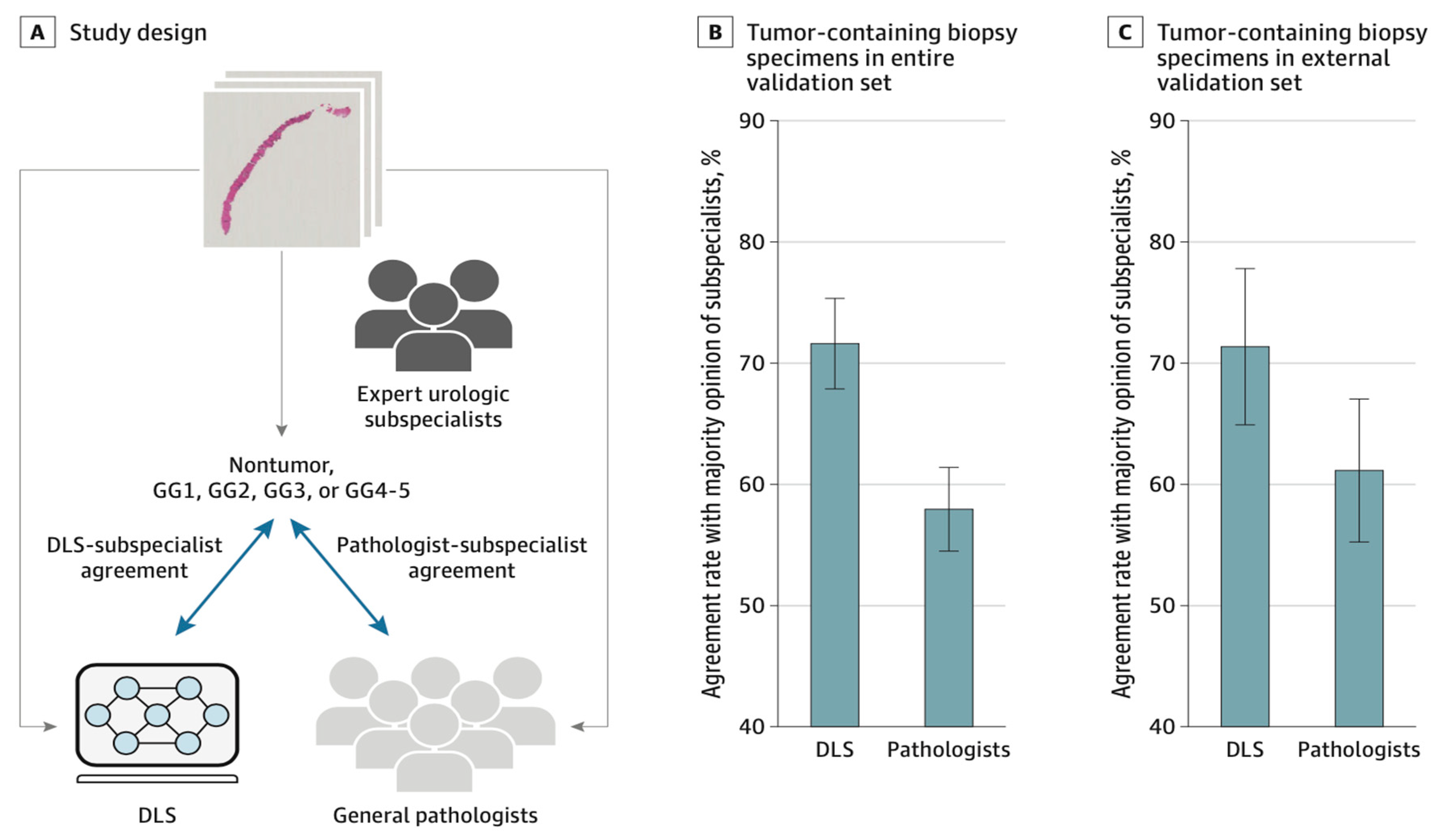
At the moment, there is a lack of clear direct comparison of CNN performance to a practical consecutive clinical cohort with high-quality data annotation and with CNN evaluating image data that includes the apparent diffusion constant as the probably most important component in prostate MRI. Some published studies examine CNN performance by using T2-weighted imaging solely or use performance metrics that cannot be directly compared with the clinical performance (for instance, the distinction of manually preselected patches of noncancerous tissues or indolent prostate cancer from clinically important prostate cancer)(Siegel, 2020). withal, the DLS showed higher proficiency than general pathologists at Gleason grading prostate needle core biopsy specimens and generalized to an independent institution as seen in (Nagpal et al., 2019) However, future research and analysis are necessary to evaluate the potential utility of exploitation the DLS as a call support tool in clinical workflows and to improve the quality of prostate cancer grading for therapy and medical decisions.

Figure 2.19. Comparison of deep learning system (DLS) and Pathologist Agreement Rates with Subspecialists at Gleason Grading of Tumor-Containing Biopsy Specimens.

Figure 2.19. Comparison of deep learning system (DLS) and Pathologist Agreement Rates with Subspecialists at Gleason Grading of Tumor-Containing Biopsy Specimens.

2.4. Summary of literature review

The Gleason score is the strongest correlating predictor of recurrence for prostate cancer but has substantial inter-observer variability, limiting its usefulness for individual patients. Specialized urological pathologists have greater concordance; but such expertise is not widely nor readily available. When trying to detect prostate cancer, Prostate-specific Antigen alone is not an accurate indicator cancer but rather, the combination with magnetic resonance imaging of the type multi-parametric sequence will contribute greatly in identification, staging and treatment monitoring of various types of tumor. The best-automated method to prostate cancer grading using artificial intelligence approach is deep learning due to its capability to identify salient characteristics which have great potential to increase the quality of Gleason grading by improving consistency and offering expert-level grading independent of location. Furthermore, the limitation of deep learning from dataset volume perspective in Gleason score prediction can be overcome using data augmentation, transfer learning and even Generative adversarial networks provide an opportunity to overcome this limitation as they can produce synthetic images which are similar to the original images. However, to date, there have been no reports in the literature on the generation of synthetic indurations.

3. Methodology Review

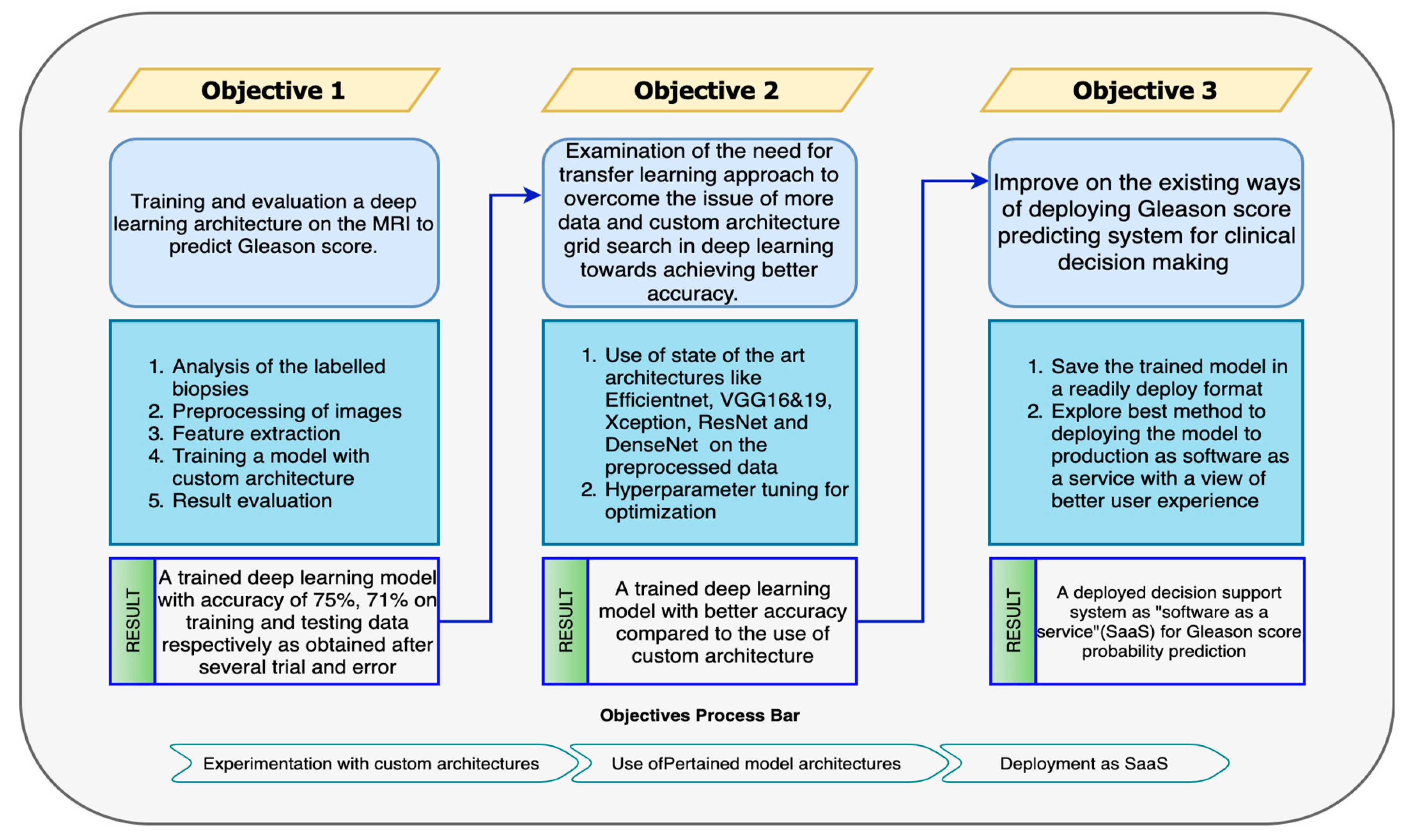
The aim of this study is to evaluate the ability of machine learning and deep learning system (DLS) to develop decision support system on Gleason score prediction for prostate cancer metastasis. The following methodology was used to achieve the aforementioned objectives:

In section 3.1, the author trained a custom CNN on analyzed, preprocessed data and extracted features and did evaluation on the model outcome.

In section 3.2, the author explores the use of transfer learning using state of the art architectures such as Efficientnet, VGG, Xception, ResNet and DenseNet by unfreezing the deep layers for new feature extraction to obtain new weights with before making prediction.

In section 3.3, the author saved the best model in deployable format and explored the best approach to having the model deployed with the view of having better user experience.

Figure 3.1. The approaches used to achieve the objectives and overall aim of the project.

Figure 3.1. The approaches used to achieve the objectives and overall aim of the project.

3.1. Custom deep learning architecture

The flexibility of how deep learning architecture are built has huge effect on the model outcome. One of the challenges in deep learning is building the best architecture for the use case. The author explored the use of deep convolutional neural network for feature extraction with artificial neural network for the predictive top layer on the preprocessed data as described in the sections below:

3.1.1. Data analysis and preprocessing

The raw data was preprocessed by creating 36 tiles with the aim to reduce the whitespace in each biopsy slide so that the model feature extraction stage can focus more on the region of cells concentration.

Figure 3.1.1a. A view of the raw data before tiles creation.

Figure 3.1.1a. A view of the raw data before tiles creation.

Figure 3.1.1b. A view of the raw data after tiles creation.

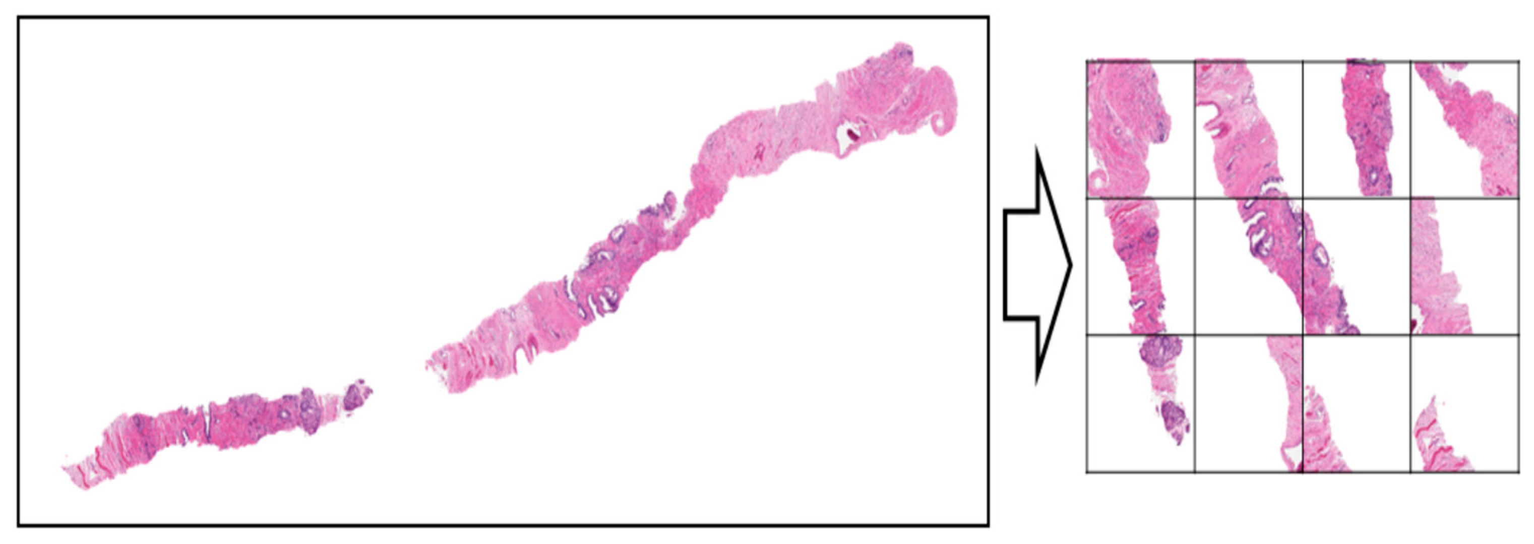
Figure 3.1.1b. A view of the raw data after tiles creation.

With the tiles created, the images are further processed into gray-scale and resized into 224 x 224. The images are channeled into filtering pipeline where the gaussian filter is applied on them for pattern spotting and recognition.

Figure 3.1.1c. A view of the preprocessing image pipeline.

Figure 3.1.1c. A view of the preprocessing image pipeline.

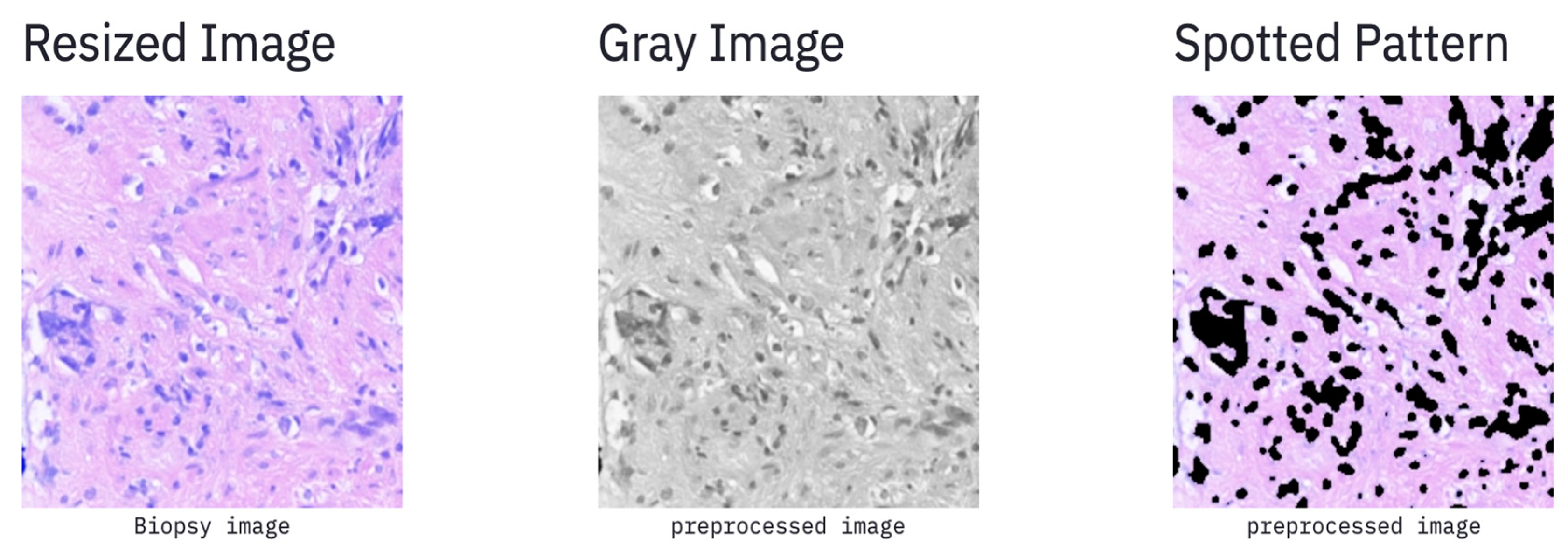
The concentration and the degree of cell metastasis in each cell sample was also explored using the masking method whereby each biopsy slide is is laid with the region of interest mask just as shown

Figure 3.1.1d. masked image for pattern spotting.

Figure 3.1.1d. masked image for pattern spotting.

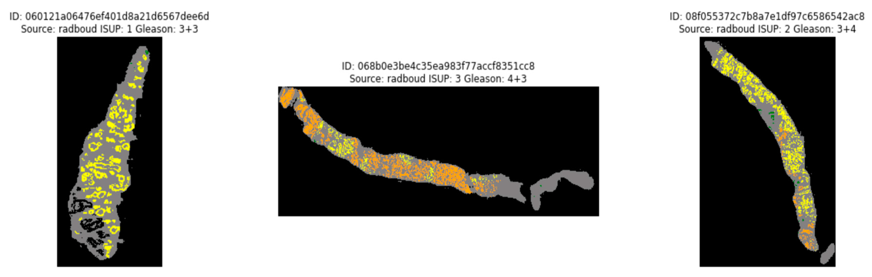
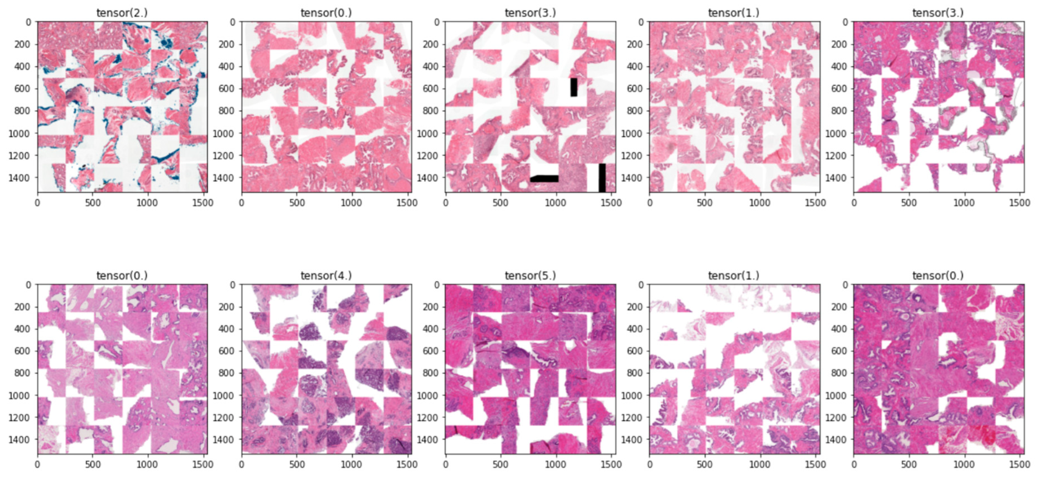
The training image labels were converted from given Gleason score which is the sum of minor and major confirmed cell metastasis concentration into discrete numbers ranging from 0-9. With this, the model can be trained on distinct number of classes and the prediction can be mapped back into Gleason score respectively. The conversion process can be seen in the figure below:

Figure 3.1.1e. Slides labels mapping.

Figure 3.1.1e. Slides labels mapping.

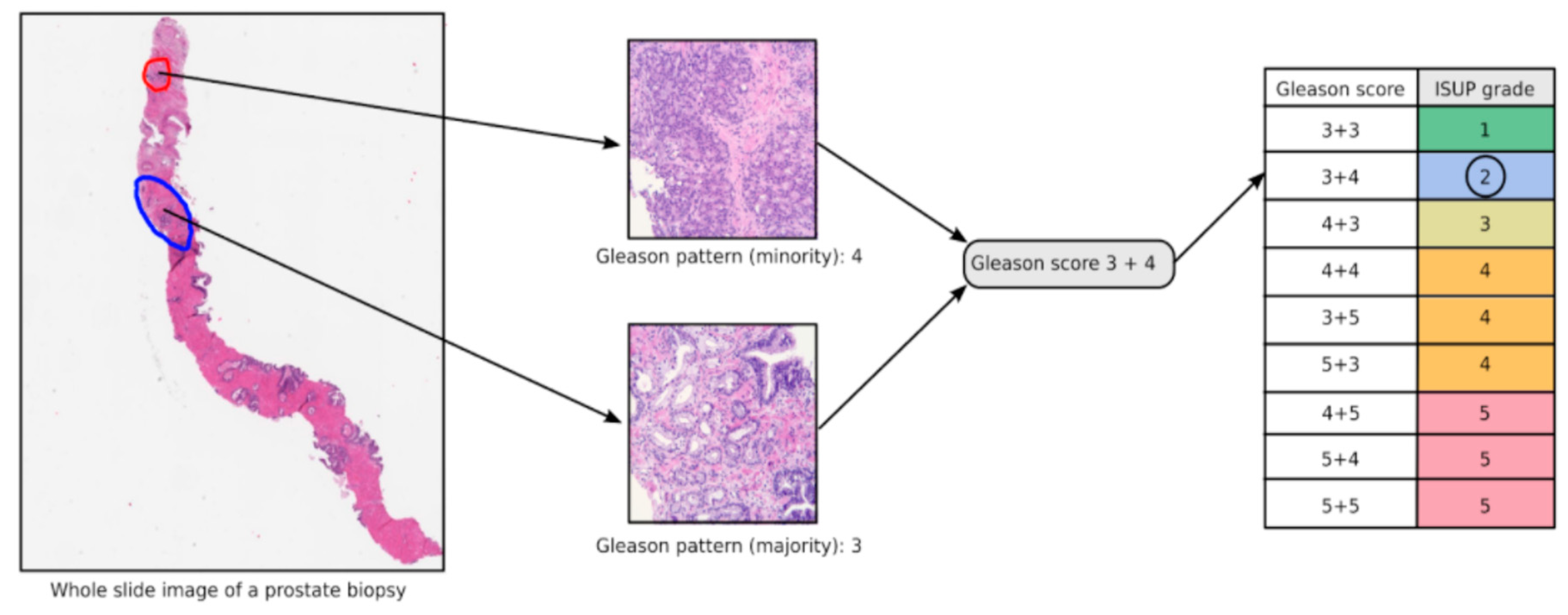
The entire preprocessed data was divided into training and testing sets using split ratio of 70:30% respectively whereby the model was fitted on the training set and the evaluated on the testing set.

3.1.2. Model training

The custom model of choice is the CNN with 32 filters to extract features and pattern spotting in the deep layer of the neural network while a simple artificial neural network was used at the top layer. The custom network architecture is shown in the figure below:

Figure 3.1.2a. Custom model architecture.

Figure 3.1.2a. Custom model architecture.

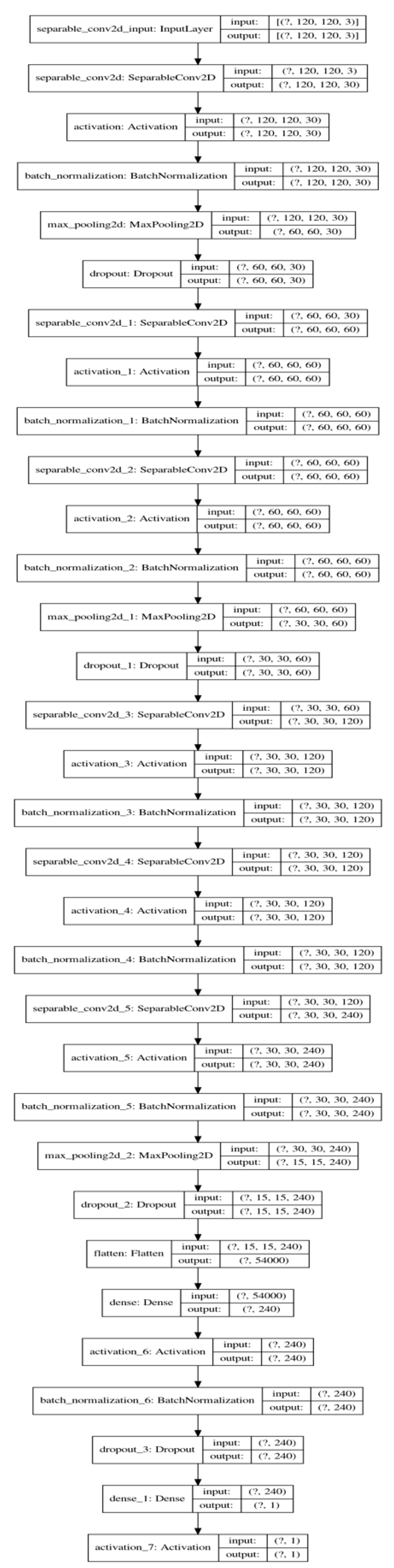
The model was compiled with the “binary_crossentropy” loss function since it’s a multi-class model and the choice of optimizer was “Adam” because of its great performance on the task. The custom model trained for 10 epochs of 100 epochs to reach a convergence discussed in the next section.

Figure 3.1.2b. Custom model training logs.

Figure 3.1.2b. Custom model training logs.

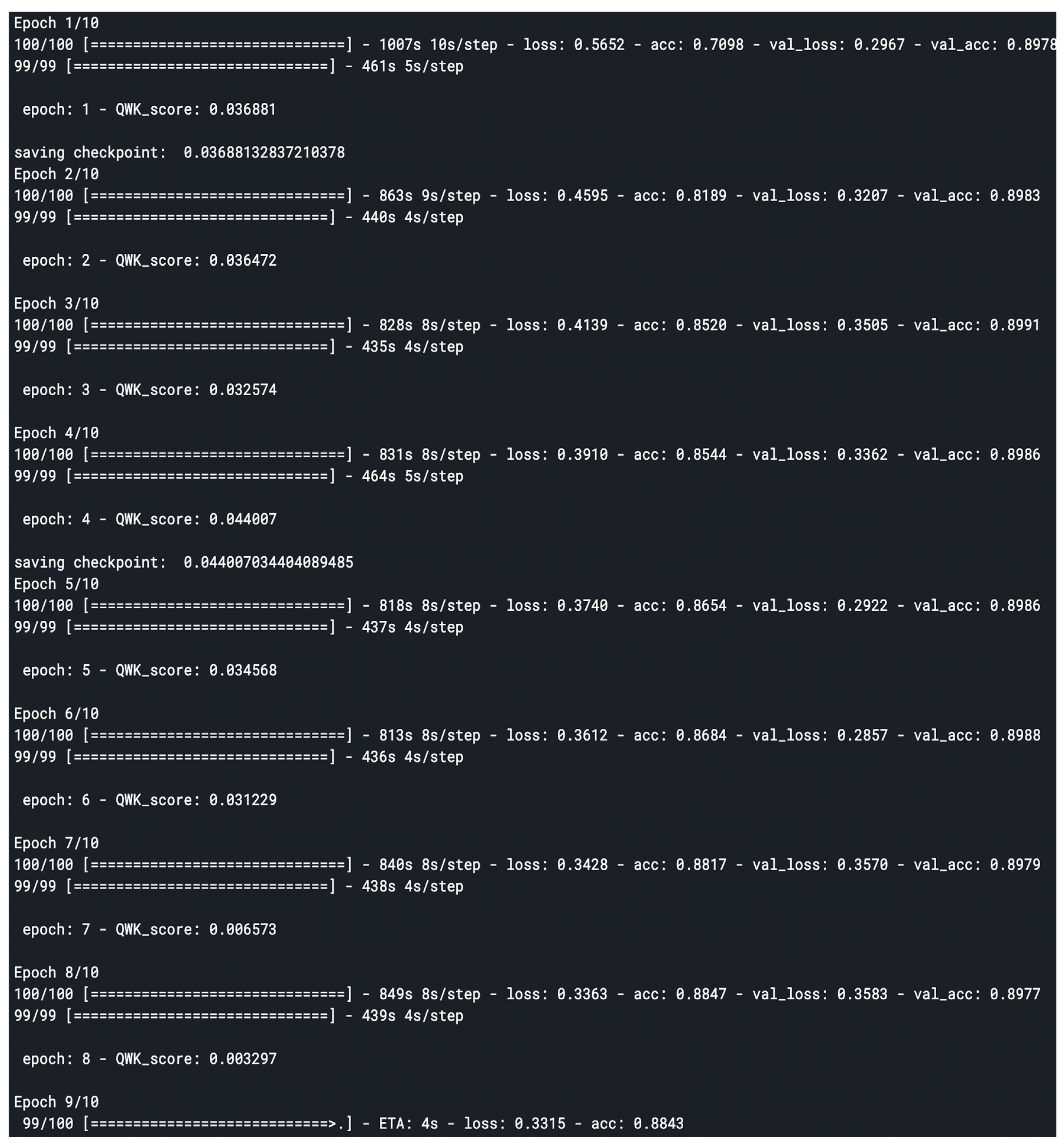
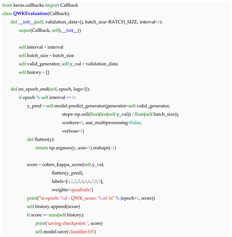
The model was evaluated using based on the quadratic weighted kappa, which measures the agreement between two outcomes. This metric typically varies from 0 (random agreement) to 1 (complete agreement). In the event that there is less agreement than expected by chance, the metric may go below 0.

The quadratic weighted kappa is calculated as follows. First, an N x N histogram matrix O is constructed, such that 𝑂_𝑖,𝑗 O_i,jcorresponds to the number of isup_grade's i (actual) that received a predicted value j. An N-by-N matrix of weights, w, is calculated based on the difference between actual and predicted values:

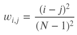
An N-by-N histogram matrix of expected outcomes, E, is calculated assuming that there is no correlation between values. This is calculated as the outer product between the actual histogram vector of outcomes and the predicted histogram vector, normalized such that E and O have the same sum.

Finally, from these three matrices, the quadratic weighted kappa is calculated as:

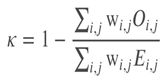where 𝑤w is the weighted matrix, 𝑂O is the histogram matrix and 𝐸E being the expected matrix.

For each epoch during training and testing, the losses were recorded and plotted against number of epochs to monitor how the model fits on the data.

3.2. Leveraging on transfer learning

One of the difficult parts of deep learning is the iterative part to finding the best architecture for a use case. The custom model built in the previous section performed at a 70% average score on the test data which is not good enough for medical decision-making system. The use of state-of-the-art architectures such as those mention earlier really boosted the model performance to 85%. The author fitted different transfer deep learning architectures on the preprocessed data by unfreezing the deep layer since all the available trained architectures are not trained on similar data. The result of the experiment is further discussed the the result and analysis section of this report.

3.3. Deployment of the system as a Software as a Service(SaaS)

The trained model is not useful except when deployed as decision support system to be interacted with on new sample biopsies whereby pathologist can easily get the corresponding Gleason score for the prostate cancer cell metastasis. This was achieved with the following:

3.3.1. Method of deployment

There are several methods to develop and deploy machine learning architectures of which some are:

• Train by batch, predict on the fly, serve via REST API: training and persisting are done offline while prediction is done in real-time.
• Train by batch, predict by batch, serve through a shared database: training and persisting are done offline while predictions are done in a distributed queue which is almost similar to a real-time prediction
• Train, predict by streaming: both training and predicting are done on different but connected streams.
• Train by batch, predict on mobile (or other clients): similar to type 1 but the prediction is made on customer gadget.

The choice of architecture for this project is the “Train by batch, predict on fly and serve via REST API. This is further discussed in the result and analysis section of this report.

3.3.2. Mode of deployment

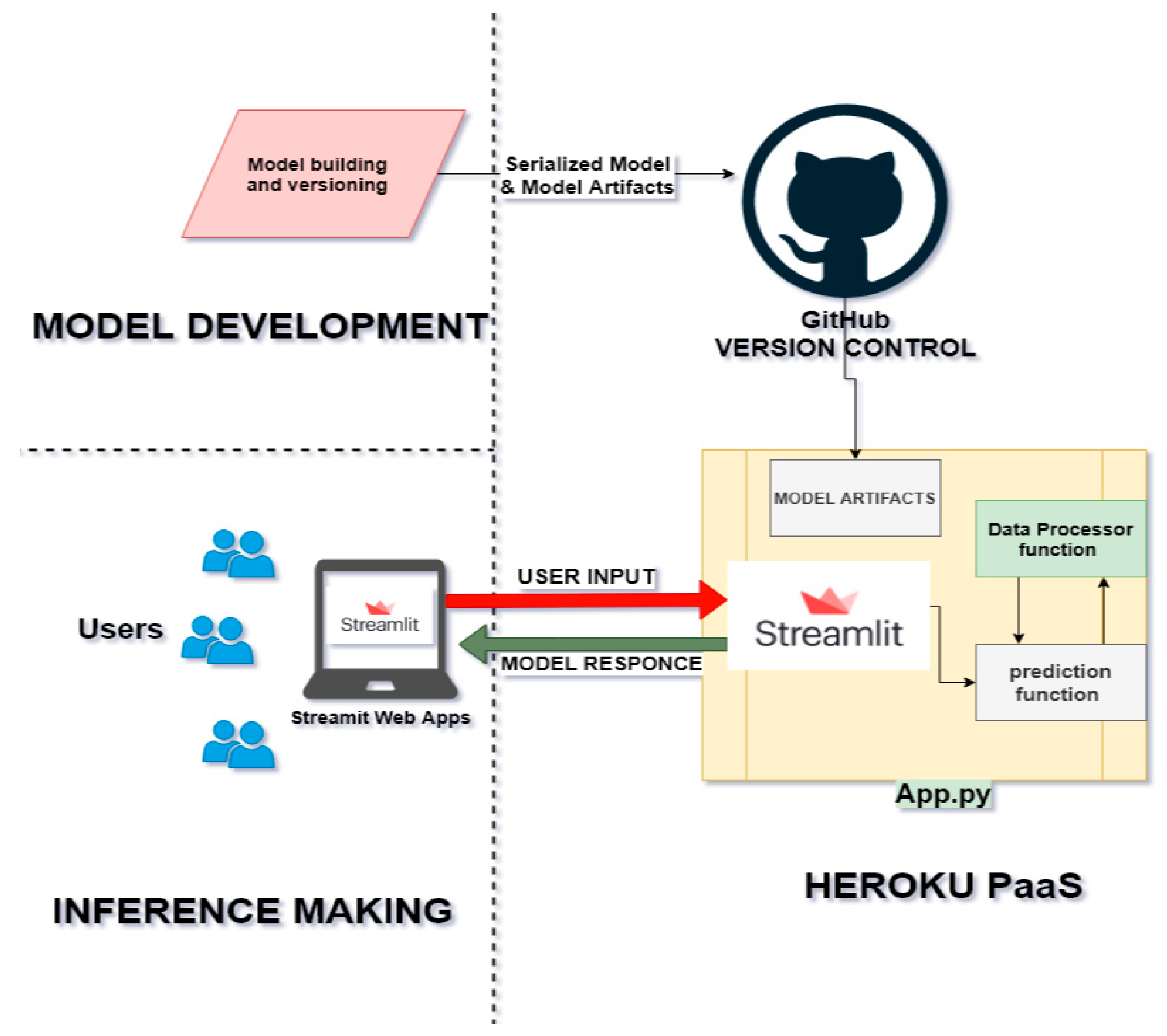
The author built a web interface to consume the model and data preprocessing pipeline API endpoints where the pathologist can upload sample tissue biopsy image and get the corresponding Gleason score immediately. This makes it easy and ready to use for many users at a time. The web application is built using Streamlit. Streamlit is an open-source app framework that provides a relatively easy way for data scientists and machine learning engineers to create beautiful, performant apps in only a few hours! It combines three ideals around embracing Python scripting, weave in interactions, and instant deployment. The web application is deployed and hosted on google cloud service for remote accessing as described in the system architecture below:

Figure 3.3.2. Deployment architecture.

Figure 3.3.2. Deployment architecture.

4. Result and Analysis

The result of this project has been demystified into major sections that made up the experiment. From data ingestions into the system to the final display of the model predictions with critical consideration of the research objectives.

4.1. Result and analysis on data preprocessing approach

Generally, in machine learning, model performance is highly dependent on how data are processed. These preprocessing on image data such as resizing, transforming, reducing and increasing number of channels etc. were experimented with the aim to get the best out of the data. The major data preprocessing steps that have significant effect on the model performance were tiles creation and filter application.

4.1.1. Tiles creation vs Raw data

The custom model was trained on the raw data and also on tiles format. Result shows that the model confidence level improved on the tiles version compared to that of the raw data. This is not surprising because the model had focus more on the concentrated region of metastasis rather than empty white spaces. This is further explained in the table below:

Table 4.1.1. model evaluation based on tiles and raw data.

Table 4.1.1. model evaluation based on tiles and raw data.

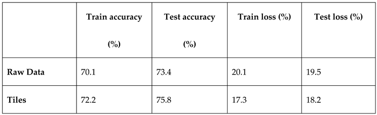From the table above, the tiles creation gave a better result than using the raw data which form the basis of the preprocessing for the entire project.

4.1.2. Gaussian filter application

The application of specific filters such as the gaussian filter at preprocessing stage also have great effect on the model performance. The filters help to reduce noise by blurring the image, increasing edge detection, etc. One advantage a Gaussian filter has over a median filter is that it's faster because multiplying and adding is probably faster than sorting. The table below shows the result of applying different filters on the biopsy:

Table 4.1.2a. model evaluation based on filters.

Table 4.1.2a. model evaluation based on filters.

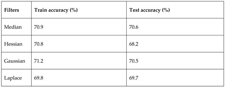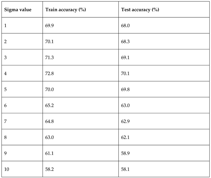
The gaussian filter outperformed other filters with default parameters. In other to further see the effect of the filter on the model, the gaussian filter sigma parameter which is the standard deviation for Gaussian kernel was varied for 10 intervals. The standard deviations of the Gaussian filter are given for each axis as a sequence, or as a single number, in which case it is equal for all axes. The result is as shown in the table below:

Table 4.1.2b. model evaluation based on sigma values.

Table 4.1.2b. model evaluation based on sigma values.

4.2. Transfer learning result and analysis

While the custom model did perform well on the data, the use of transfer learning architectures could not be exempted. We trained and compare some state-of-the-art architectures by unfreezing the deep layers to obtain new weights. Most of these architectures performed better than the custom model as they have more trainable parameters. The table below shows the result of this analysis in details:

Table 4.2. result analysis of transfer learning.

Table 4.2. result analysis of transfer learning.

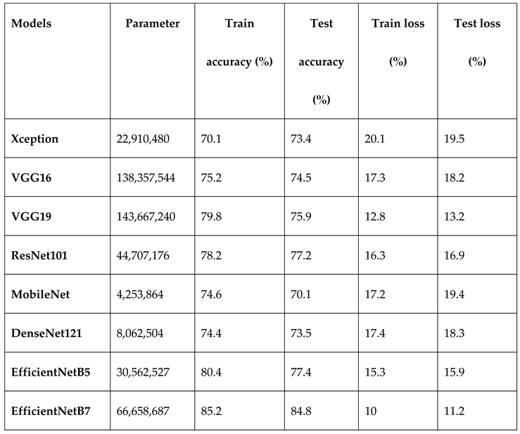Figure 4.2a. train and test accuracy analysis .

Figure 4.2a. train and test accuracy analysis .

Figure 4.2b. train and test loss analysis.

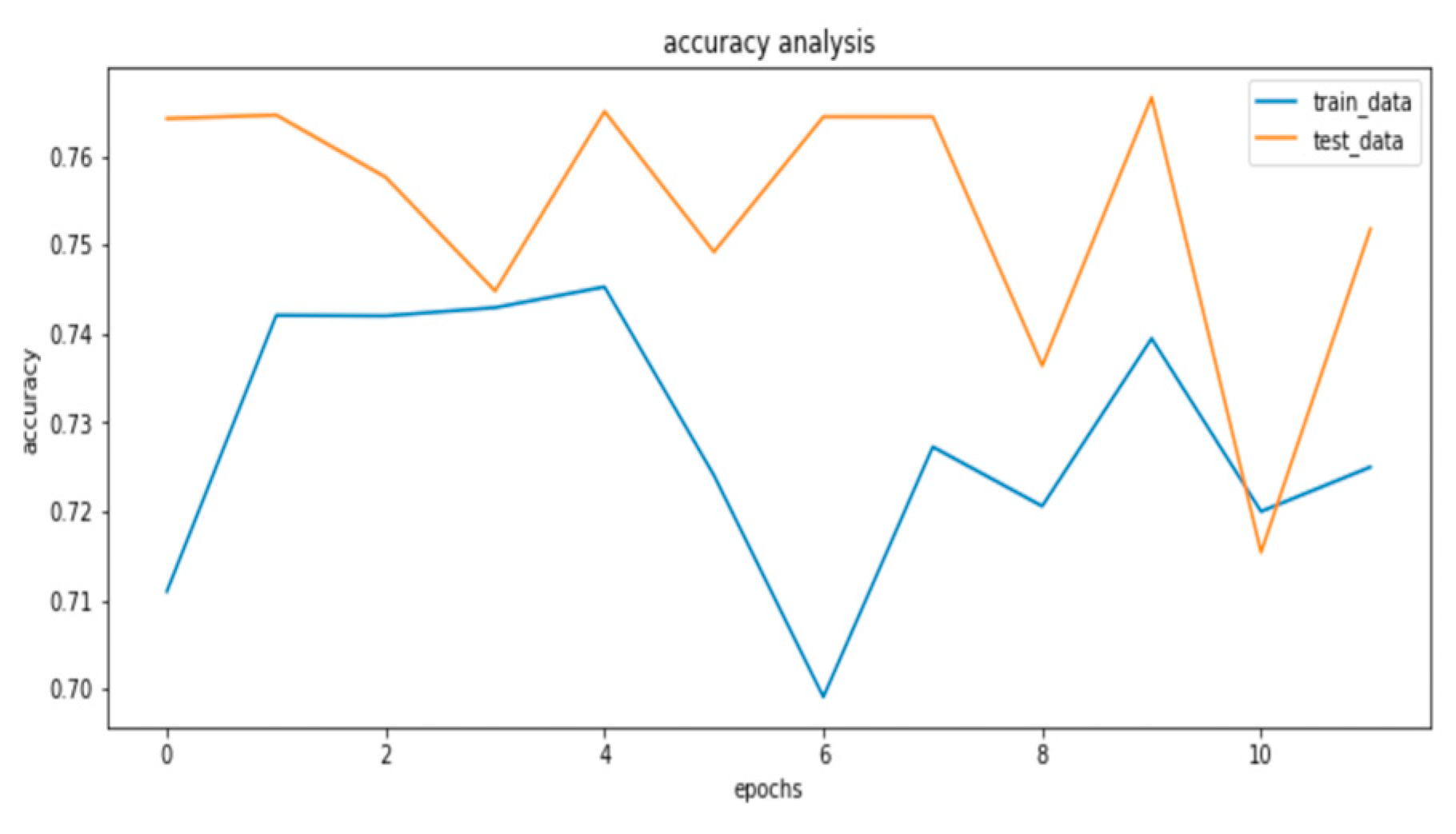
Figure 4.2b. train and test loss analysis.

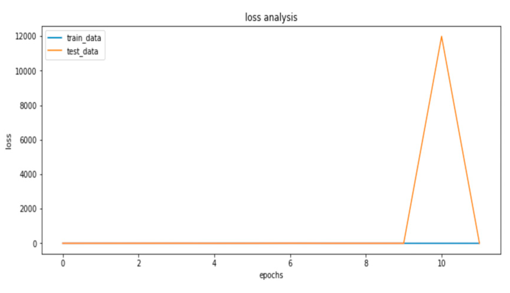
From the analysis above, the EfficientNetB7 performed best on the data and as such, this model is saved and deployed for utilization.

4.3. Web application deployment and usage result and analysis

The utilization of the built model as a decision support system is the major goal of this project. The choice of deployment as discussed in the methodology of this report is further analyzed below:

Table 4.3a. model deployment patterns .

Table 4.3a. model deployment patterns .

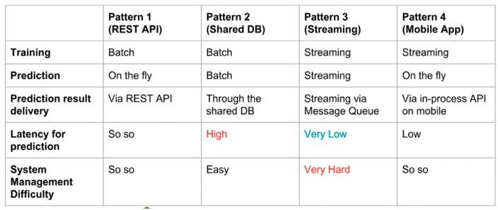The adopted pattern 1 so that each biopsy can have corresponding Gleason score upon request and to decouple the backend of the system from the frontend for easy optimization and upgrading in the nearest future. Most similar software applications that tend to solve the same problem have a common issue know as tightly coupled dependencies which makes this solution a better approach to Gleason score prediction decision support system.

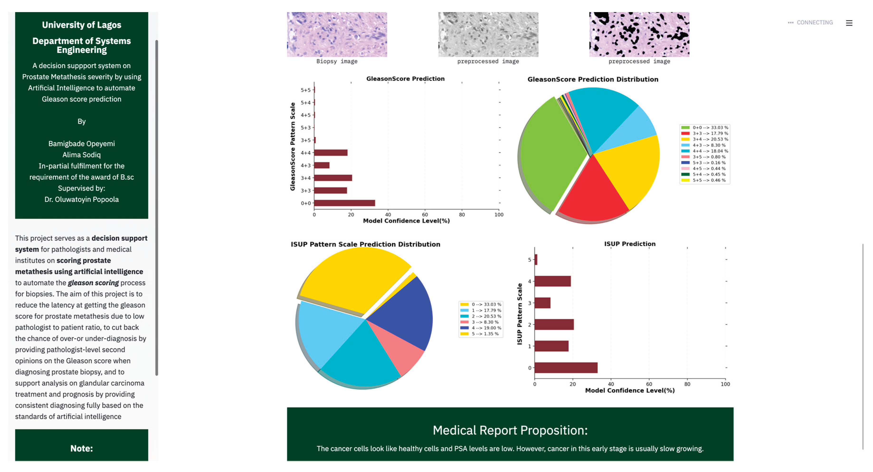
The user interface was built with user experience priorities. The result of the system is displayed in human readable formats (Gleason confidence level and ISUP) with the use chats for easy interpretation just as displayed below:

Figure 4.3. Decision support system.

Figure 4.3. Decision support system.

5. Conclusion and Recommendation

The aim of this study was to evaluate the ability of deep learning architectures and models on microscopic scan of tissues as a means of automating the grading of diagnostic prostate biopsy specimens on Gleason scale through the predictive capability of artificial intelligence on which a decision support system can be built on for the compensation of low pathologists to patients ratio in the world. It has become evident that the use of state-of-the arts deep learning architectures are faster at reaching a convergence in desired results than the use custom architectures. This is because of the flexibilities at which this model architectures can be constructed and the experimentation time cost. Also, the preprocessing steps involved in the images can have great influence on the model performance since the neural weights are learnt from the data. The use of some specific filters such as the gaussian contribute greatly to model performance compared to original images.

It is suggested that the accuracy and comprehensiveness of this model be assessed in future work. Subsequently, a better classification network should be trained using the more microscopic images or magnetic resonance images and tested on vetted patient’s data to determine the viability of using artificial intelligence and experts’ views for Gleason score prediction

The use of machine learning has the capability to standardize the Gleason score prediction which can serve as a decision support system in the medical industry.

References

- Brunese, L., Mercaldo, F., Reginelli, A., & Santone, A. (2020). Formal methods for prostate cancer Gleason score and treatment prediction using radiomic biomarkers. Magnetic Resonance Imaging, 66, 165–175. [CrossRef]
- Chaddad, A., Niazi, T., Probst, S., Bladou, F., Anidjar, M., & Bahoric, B. (2018). Predicting Gleason score of prostate cancer patients using radiomic analysis. Frontiers in Oncology, 8(DEC), 1–10. [CrossRef]
- Citak-Er, F., Vural, M., Acar, O., Esen, T., Onay, A., & Ozturk-Isik, E. (2014). Final Gleason score prediction using discriminant analysis and support vector machine based on preoperative multiparametric MR imaging of prostate cancer at 3T. BioMed Research International, 2014. [CrossRef]
- Cruz, J. A., & Wishart, D. S. (2006). Applications of Machine Learning in Cancer Prediction and Prognosis. 59–77.
- Free PSA: Test, results, and prostate cancer. (n.d.). Retrieved September 20, 2020, from https://www.medicalnewstoday.com/articles/322001#understanding-the-free-psa-test.
- Liu, S., Zheng, H., Feng, Y., & Li, W. (2017). Prostate cancer diagnosis using deep learning with 3D multiparametric MRI. Medical Imaging 2017: Computer-Aided Diagnosis, 10134, 1013428. [CrossRef]
- Liu, Y., & An, X. (2018). A classification model for the prostate cancer based on deep learning. Proceedings - 2017 10th International Congress on Image and Signal Processing, BioMedical Engineering and Informatics, CISP-BMEI 2017, 2018-Janua, 1–6. [CrossRef]
- Nagpal, K., Foote, D., Liu, Y., Chen, P. C., Wulczyn, E., Tan, F., Olson, N., Smith, J. L., Mohtashamian, A., Wren, J. H., Corrado, G. S., Macdonald, R., Peng, L. H., Amin, M. B., Evans, A. J., Sangoi, A. R., Mermel, C. H., Hipp, J. D., & Stumpe, M. C. (2019). Development and validation of a deep learning algorithm for improving Gleason scoring of prostate cancer. Npj Digital Medicine, June. [CrossRef]
- Prostate cancer - Symptoms and causes - Mayo Clinic. (n.d.). Retrieved September 13, 2020, from https://www.mayoclinic.org/diseases-conditions/prostate-cancer/symptoms-causes/syc-20353087.
- Roberts, M. J., Teloken, P., Chambers, S. K., Williams, S. G., Yaxley, J., Samaratunga, H., Frydenberg, M., & Gardiner, R. A. (‘Frank’). (2000). Prostate Cancer Detection. In Endotext. MDText.com, Inc. http://www.ncbi.nlm.nih.gov/pubmed/25905271.
- Ryu, H. S., Jin, M. S., Park, J. H., Lee, S., Cho, J., Oh, S., Kwak, T. Y., Isaacwoo, J., Mun, Y., Kim, S. W., Hwang, S., Shin, S. J., & Chang, H. (2019). Automated gleason scoring and tumor quantification in prostate core needle biopsy images using deep neural networks and its comparison with pathologist-based assessment. Cancers, 11(12). [CrossRef]
- Siegel, C. (2020). Re: Classification of Cancer at Prostate MRI: Deep Learning versus Clinical PI-RADS Assessment. The Journal of Urology, 204(3), 597. [CrossRef]
- Thomas, B. L. (n.d.). Transurethral biopsy. 17 mm, 1–5.
- Vargas, H. A. (2014). Prostate Cancer Aggressiveness : Assessment with Whole-Lesion Histogram Analysis of the Apparent. 271(1), 143–152.
- Yoo, S., Gujrathi, I., Haider, M. A., & Khalvati, F. (2019). Prostate Cancer Detection using Deep Convolutional Neural Networks. Scientific Reports, 9(1), 1–10. [CrossRef]
- Zhang, Y., Zhang, J., Song, Y., Shen, C., & Yang, G. (n.d.). Gleason Score Prediction using Deep Learning in Tissue Microarray Image. 1–8.
- Lee, J.-G., Jun, S., Cho, Y.-W., Lee, H., Kim, G.B., Seo, J.B. & Kim, N. 2017. Deep Learning in Medical Imaging: General Overview. Korean journal of radiology. 18(4):570-584. [CrossRef]
- Lakhani, P., Gray, D., Pett, C., Nagy, P. & Shih, G. 2018. Hello World Deep Learning in Medical Imaging. Journal of Digital Imaging. 31(3):283-289. Journal of Digital Imaging. [CrossRef]
- Wong, S.C., Gatt, A., Stamatescu, V. & McDonnell, M.D. 2016. Understanding data augmentation for classification: when to warp? Cornell University Library.
- Tajbakhsh, N., Shin, J., Gurudu, S., Hurst, R., Kendall, C., Gotway, M. & Liang, J. 2016. Convolutional Neural Networks for Medical Image Analysis: Full Training or Fine Tuning? IEEE Transactions On Medical Imaging. 35(5):1299-1312. [CrossRef]
Disclaimer/Publisher’s Note: The statements, opinions and data contained in all publications are solely those of the individual author(s) and contributor(s) and not of MDPI and/or the editor(s). MDPI and/or the editor(s) disclaim responsibility for any injury to people or property resulting from any ideas, methods, instructions or products referred to in the content. |
© 2024 by the authors. Licensee MDPI, Basel, Switzerland. This article is an open access article distributed under the terms and conditions of the Creative Commons Attribution (CC BY) license (http://creativecommons.org/licenses/by/4.0/).
Copyright: This open access article is published under a Creative Commons CC BY 4.0 license, which permit the free download, distribution, and reuse, provided that the author and preprint are cited in any reuse.