
Submitted:
29 January 2024
Posted:
30 January 2024
You are already at the latest version
Abstract
In steel recycling, the optimization of electric arc furnaces (EAFs) is of central importance in order to increase efficiency and reduce costs. This study focuses on the optimization of electric arcs, which make a significant contribution to the energy consumption of EAFs. A three-phase equivalent circuit integrated with the Cassie-Mayr arc model is used to capture the nonlinear and dynamic characteristics of arcs, including arc breakage and ignition process. A particle swarm optimization technique is applied to real EAF data containing current and voltage measurements to estimate the parameters of the Cassie-Mayr model. A novel Arc Quality Index (AQI) is introduced in the study, which can be used to evaluate arc quality based on deviations from optimal conditions. The AQI provides a qualitative assessment of arc quality, analogous to indices such as arc coverage and arc stability. The study concludes that the AQI serves as an effective operational tool for EAF operators to optimize production and increase the efficiency and sustainability of steel production. The results underline the importance of understanding electric arc dynamics for the development of EAF technology.
Keywords:
electric arc furnace
; Cassie-Mayr
; particle swarm optimization
; arc model
; equivalent circuit
1. Introduction
Steel, a fundamental material in numerous industries such as construction, manufacturing and energy, was produced in the order of 1.9 billion tons worldwide in 2022 [1]. Despite its widespread benefits, steel production is associated with significant environmental problems, in particular high energy consumption and significant emissions. With steel demand expected to increase by 30% over the next three decades, there is an urgent need for more sustainable production methods [2]. Electric Arc Furnaces (EAFs) offer a promising solution as they enable steel production from scrap steel and direct reduced iron (DRI). In addition, recent advances in EAF technology have led to improvements such as shorter tap-to-tap times, lower energy consumption through the introduction of carbon monoxide post-combustion and melt stirring techniques. Furthermore, digitalization and the application of advanced technologies, e.g., machine learning, have shown great potential for further optimization of the steel production process, i.e., temperature soft sensors [3] and slag foaming estimation [4]. These technologies enable the analysis and utilization of large datasets and provide valuable insights for optimizing production parameters and reducing environmental impact. In the metallurgical industry, especially in the EAF operation, accurate real-time measurements of key performance indicators (KPIs) are essential for high productivity. However, challenges such as cost and data acquisition limitations often hinder the direct measurement of critical variables. Soft sensors, which use indirect measurements to estimate hard-to-measure process variables, have proven to be a cost-effective and adaptable solution. These models, ranging from fuzzy [3] and neural network models [4] to comprehensive theoretical models [5,6,7,8,9], are central to improving process control and plant efficiency.
One of the critical aspects of three-phase alternating current (AC) EAFs is the architecture of the power supply system, depicted in Figure 1. This system consists of a series of components, starting with the intake of electric power from the utility grid, referred to as . At the point of common coupling (PCC), which is characterized by the short-circuit resistance and the inductance , the grid is connected to a high/medium voltage step-down transformer (HV/MV T1). The secondary side of HV/MV T1 then feeds into the arc furnace transformer, a medium/low voltage transformer (MV/LV T2), via a series reactor which serves to increase the overall reactance of the system [10]. The MV/LV T2 is equipped with a variable tapping mechanism that makes it possible to adjust the turns ratio under load and thus regulate the voltage supplied to the EAF. The measuring point (MP) is located on the secondary side of the arc furnace transformer and enables the measurement of the line-to-ground voltages and line currents. The line current flows through conductors consisting of flexible cables and tubular conductors leading to the graphite electrodes, which are modeled as reactance R and inductance L. At the point where these electrodes meet the conductive metal scrap, an electric arc is formed, which closes the circuit that is grounded via the furnace hearth. The dynamic control of the arc intensity is ensured by the precise vertical adjustment of the electrodes. This adjustment is performed by an electrode control system designed to maintain specific current or impedance parameters for each line [11].
In an effort to increase efficiency and reduce operating costs of the EAFs, great attention is being paid to optimizing the electric arcs, which are responsible for a significant portion of the energy consumption. It is estimated that around 80% of the energy emitted by an electric arc occurs as radiation [5]. This underlines the importance of directing this radiation to the heating of scrap and molten steel rather than letting it dissipate on the furnace roof and cooling panels. The intensity of arc radiation is directly proportional to arc length and voltage, which means that longer arcs generally emit more radiation. However, longer arcs can affect stability and lead to increased radiation dispersion away from the melt. The use of foaming slag is therefore crucial for the complete coverage of arcs to minimize radiation losses and improve energy transfer to the molten metal [12], as well as to stabilize the arc’s burning behavior and increase the efficiency of the power input [13]. A major challenge is to accurately measure the coverage of the arc by slag, as direct visual access is not possible and the installation of sensors inside the furnace is impractical [14]. Various methodologies, such as laser vibrometry [4,14], imaging through the slag gate [4] and analyzing the secondary side transformer voltage [15] and current [13] have been explored. One notable approach is the use of a laser vibrometer to measure real-time vibrations of the furnace shell in combination with the operator’s estimation of arc coverage. This data is then used to train an artificial neural network that estimates the arc coverage [14]. However, it is important to note that these estimates depend on the experience of the operator. In addition, Martell et al. [15] have proposed an arc coverage index based on the third and ninth harmonic values of the voltage between the virtual-neutral and ground. While this index provides a general assessment of arc coverage, it does not provide insight into individual arc coverage. Furthermore, Sedivy et al. [13] proposed an index for foaming slag that suggests an inverse relationship to the Total Harmonic Distortion (THD) of the current. Finally, Son et al. [4] developed a long short-term memory (LSTM) neural network model for estimating slag foaming height in EAF steelmaking by integrating preprocessed EAF heat data with reference data from measured furnace shell vibration and digital imaging [4]. However, a critical challenge is estimating the height of the foaming slag from images taken through the slag gate. This process is inherently complex as the initial level of the molten metal surface is indeterminate, making the accurate determination of the height of the slag foam much more difficult.
Another crucial aspect of the EAF operation is arc stability, which significantly affects both electrical phenomena and operational power level. Arc instability can affect the system’s ability to deliver high-power, leading to operational inefficiencies. Conversely, stable arcs enable higher power output, resulting in shorter tapping times, higher productivity and steel quality [16]. Various methodologies have been used to evaluate arc stability, including analysis of secondary-side transformer voltages or line currents [15,16,17] and the evaluation of acoustic signals [18]. An important stability indicator in the frequency domain is the THD of the voltage or current signal [17]. THD values vary in the different EAF heating stages and generally show increased values during the initial bore-down and early melting stages, which then decrease during the refining stages. Martell et al. [16] have introduced a stability index based on the RMS voltage between the virtual-neutral of the EAF delta transformer and ground. In addition, arc stability can be evaluated by analyzing acoustic signals, where a stability index is derived by examining both the time and frequency domain of these signals [18]. Arc stability is not only a reflection of the electrical behavior in the furnace, but also a crucial process variable that, together with the specific heat stage, determines the EAF’s operational power level. Understanding and controlling arc stability is critical to operational efficiency as it allows the power profile to be adjusted to the stability conditions of the arc. Effective control strategies in this area require comprehensive arc models. A variety of approaches to arc modeling can be found in the literature, including linear and nonlinear, static and dynamic methods that include both time-variant and invariant aspects as well as black-box and white-box approaches [19]. The following sections provide an overview of these arc models and explain their application and effectiveness in the operation of EAF.
The origins of arc models can be traced back almost a century, with Cassie’s model being introduced in 1939 [20] and Mayr’s model in 1943 [21]. The Mayr model was developed specifically for low-current applications and is particularly effective in the zero-crossing region, whereas the Cassie model is more suitable for high-current situations. The relatively simple Cassie and Mayr differential equation models can effectively model the key characteristics of the arc as a circuit element, with arc resistance defined as a dynamic variable. Based on the simplifications of principal power-loss mechanisms and energy storage in the arc column, they serve as valuable tools to understand arcing phenomena. In an effort to develop more comprehensive models, several approaches have been proposed to merge the arc models of Cassie and Mayr. One approach is to use a current-based transition function, where a Mayr model is active near zero current, while the Cassie arc model is active at higher currents [22,23]. Another possibility is to generalize the Cassie and Mayr arc model by introducing an additional parameter denoted as [19,24,25]. Setting to zero yields the Mayr model, while setting it to one produces the Cassie model. The theoretical range for is between 0.5 and 1, as stated by Lee et al. [24], although it is worth noting that experimental data suggests that values greater than one are possible. Khakpour et. al [26] proposed an improved Mayr arc model in which the dissipated power at current passage through the zero point was defined in terms of the arc current and the estimated arc diameter. The hyperparameters of the arc model were then estimated using measurements from a dedicated experimental setup. In addition to the EAFs, the circuit breaker models [27,28,29,30,31] also utilize the arc models with more advanced adaptations of Mayr’s and Cassie’s models, i.e., the Schwarz arc model, the Habedank arc model and the KEMA arc model [30,31]. However, these models introduce additional parameters, which makes their identification even more difficult.
In 1990, Acha et al. [32] introduced a novel arc modeling methodology known as the power balance equation. This dynamic arc model is based on a system of differential equations, collectively referred to as the power balance equation. The basic premise of this approach revolves around establishing an equilibrium in which the total power generated in the arc equals the power dissipated to the surroundings and the power contributing to the arc’s internal energy. The radius of the arc is chosen as the state variable and forms the core of the differential equation. In recent years, increasing attention has been paid to analyzing and determining the parameters inherent in the power balance equation. Various methodologies have been explored, including analytical solutions [33,34], as well as optimization techniques such as Monte Carlo [35], genetic algorithms [35,36,37] and particle swarm optimization [36]. In addition, efforts have been made to understand the stochastic properties of these parameters using approaches such as the ARIMA model [35] and the LSTM neural network [37]. In the paper [33] it has been found that the parameters significantly change during the EAF stages, i.e., melting stage and the refining stage. However, it is worth noting that these methods often restrict the power balance equation to a particular scenario characterized by the values and .
MagnetoHydroDynamic (MHD) models represent the most complete type of plasma modeling and provide comprehensive insights into the behavior of electric arcs. These models require the solution of a complex set of differential equations that include Maxwell’s equations, the Navier-Stokes equations modified by the Lorentz force, and the energy equations that account for the Joule heating effect [38]. MHD theory was also applied to understand the parameter values of the Cassie-Mayr hybrid arc model [23]. However, despite their thoroughness, a major challenge in MHD modeling is the scarcity of precise data on the physical properties of the plasma gas. Furthermore, the need for fine discretization in these models, which is essential for accurate system estimations, leads to significant computational requirements, making industrial real-time applications a challenge. In response, Channel Arc Models (CAM) were developed as a more computationally tractable alternative. These models introduce several simplifications to reduce complexity. Key assumptions include the establishment of a local thermodynamic equilibrium, the conception of the arc as an ionized gas channel with axial symmetry, and the homogeneity of current and temperature distributions across the channel diameter [39,40,41]. Although CAM are less complex than MHD models, they still pose the task of estimating numerous model parameters. While this parameter estimation requirement is less daunting than for MHD models, it remains a non-trivial aspect of channel arc modeling that affects both the accuracy of the model and its applicability in various industrial scenarios.
This article presents a holistic approach for the electrical analysis of three-phase AC EAF and introduces a novel Arc Quality Index (AQI) based on the Cassie-Mayr arc model. The approach is based on a three-phase equivalent circuit that integrates the Cassie-Mayr arc model to capture the nonlinear and time-varying load characteristics of electric arcs. The model also takes into account the processes of arc breakage and ignition, thus improving the accuracy in representing the dynamic behavior of arcs, especially during the chaotic melting stage. The parameters of the Cassie-Mayr arc model, in particular the arc time constant and the Cassie-Mayr constant for each electrode, are determined using a particle swarm optimization technique. This estimation is performed using real furnace data collected during a single heat that included both the melting and refining stages. The optimization objective or fitness function is defined by minimizing the discrepancy between the harmonic content of the measured and simulated voltage and current signals. The AQI is formulated based on the deviations from the optimum conditions utilizing the Cassie-Mayr arc parameters and the RMS value of arc resistance. This index provides a thorough qualitative assessment of arc quality, analogous to indices such as the arc coverage index and the arc stability index. In addition, the AQI is based solely on the measurements of current and voltage, which can be measured on-site to assess arc quality. Effective monitoring and control of the AQI enables operators to improve the operation of the EAF and thus increase the efficiency of steel production. Achieving high AQI values is desirable, at least in the later stages of EAF operation, in order to minimize energy losses caused by radiation. At this point, the extent of arc coverage by slag proves to be a decisive factor for the AQI value and the overall EAF. Consequently, operators can take targeted measures to improve AQI, including adjustments to reduce arc length and initiatives to increase slag height, thereby optimizing operating conditions and energy utilization. This research demonstrates the importance of understanding arc dynamics in EAFs to promote more efficient and sustainable steel production techniques. Contributions of the work include: the development of a holistic electrical circuit for EAF based on the Cassie-Mayr arc model, an optimization method for parameter estimation of the Cassie-Mayr model across all three lines, and the formulation of a novel arc quality index that integrates aspects of arc stability and coverage.
2. Materials and Methods
2.1. Electric Arc Furnace (EAF)
This chapter provides a comprehensive overview of the EAF, emphasizing its crucial role in the recycling of scrap steel. In the EAF methodology, scrap steel is melted and then overheated to a target temperature, which is mainly achieved by electric arcs. These arcs form between the tips of the graphite electrodes and the scrap material. The EAF process utilizes the intense heat generated by the conductive channels, supplemented by additional heat from exothermic reactions that occur in various chemical processes. The EAF process can be divided into four main stages:
- 1.
- Charging: Normally, the furnace is fed in stages with two to four baskets of preheated scrap steel. The initial aim is to melt the first basket quickly, as this enables a more stable formation of the arcs. The subsequent baskets are added gradually to reduce the overall load on the power grid and speed up the melting process.
- 2.
- Melting: The melting stage begins with the ignition of the electric arcs, which is triggered by a brief contact between the graphite electrodes and the scrap. When the first electrode touches the scrap, the electrical circuit is not yet closed. Only when the second electrode also comes into contact does the circuit close and the first arcs are ignited. Thermochemical processes, in particular the oxidation of natural gas, play an important role in supporting the melting stage.
- 3.
- Refining: During refining, the molten steel is purified by removing impurities and dissolved gasses. The injection of oxygen is an important aspect of this stage as it allows reactions with various elements to form oxides that separate from the steel into the slag. In addition, the bath temperature is overheated up to the required values. In modern EAF operations, the refining stage is increasingly being integrated into the melting process in order to shorten tap-to-tap times.
- 4.
- Tapping: After melting, the temperature and composition of the steel are evaluated against the requirements for casting. The final steps of the EAF process include the deslagging process, followed by transportation of the molten steel to the next processing station.
2.2. Three-Phase Equivalent Circuit
In AC EAFs, the power supply is provided by a three-phase arc furnace transformer (T2). The primary winding of the T2 is normally delta-connected, while the secondary winding can be either star or delta-connected. The delta connection is often preferred as it reacts better to unbalanced loads and significantly reduces the phase currents. More precisely, the phase currents (coil currents) are reduced by a factor of compared to the line currents. With this configuration, higher line currents can be absorbed without compromising the integrity of the system. This study focuses on an equivalent circuit diagram representing the system from the perspective of the secondary side of the arc furnace transformer. Figure 2 shows a simplified equivalent circuit derived from a more complex setup shown in Figure 1. The circuit receives power from the grid, first via a step-down transformer and then via the arc furnace transformer. In this circuit configuration, the secondary phase voltages in the delta connection are labeled and are subject to variation depending on the transformer tap position. To determine the equivalent transformer resistances and inductances , all circuit elements form the primary side of T2 are viewed from the perspective of the T2 secondary side. The line currents, shown as , flow through the electrodes into the melt, which is grounded by the furnace hearth. The resistances and inductances of the flexible cables and tubular conductors leading to the electrode tips are shown as and , respectively. The electric arcs between the electrodes and the scrap or the steel bath are characterized by variable arc resistances symbolized by .
In the equivalent circuit model, the notation is standardized as follows: Voltages and currents are denoted by u and i, respectively. Capital letters stand for phasors, which represent complex variables. The real part of a phasor is extracted as . Vectors and matrices are marked in bold. Resistances and inductances are symbolized by R and L, respectively. Complex impedances are expressed as , where X is the reactance defined by the equation . Here, is the angular fundamental frequency, which is related to the fundamental frequency of the network as follows: . The secondary transformer voltages are assumed to be symmetrical and are defined as follows:
where the refers to the effective low voltage, which depends on the tap position T, and stands for the initial phase angle. Note that the sum of transformer voltages is zero: . To determine the equivalent resistances and inductances , the analysis is carried out from the secondary side of transformer T2. This means that all elements from the primary side of T2 must be reflected to the secondary side. The short-circuit power at the PCC, referred to as , is strongly dependent on the state of the grid and is treated as a simulation parameter. The utility impedance is determined as follows:
where stands for the effective high voltage at the PCC. The values of short-circuit resistance and reactance values are derived from the reactance/resistance ratio as follows:
The impedance of the step down transformer (T1) is calculated as follows:
where represents the percentage impedance, a standardized measure of the impedance of the transformer in relation to its rated power. is the rated apparent power of T1. Equations (5) and (6) are used to determine the short circuit resistance and reactance of T1, using a reactance/resistance ratio of . The turns ration of T1 is defined as , where the stands for middle voltage. The impedance of the arc furnace transformer (T2) is calculated as follows:
where represents the percentage impedance, dependent on the tapping position. is the rated apparent power of T2. Equations (5) and (6) are used to determine the short circuit resistance and reactance of T2, using a reactance/resistance ratio of . The turns ration of T2 is defined as . The equivalent resistances and equivalent inductances in the circuit, which are denoted by and respectively, are determined as follows:
where stands for the indices corresponding to all phases of the circuit. The arc transformer in this study is configured in the vector group Dd0. Consequently, the impedance values are scaled by a factor of three due to the wye-delta transform.
In the analysis of the circuit presented in Figure 2, the state variables , and are chosen, represented as . Using Kirchhoff’s current law, the remaining currents are determined by the following equations:
Applying Kirchhoff’s voltage law, we derive the relationship between inductances, resistances and the voltage sources as follows:
where the input vector is defines as and is defined as follows:
while and are defined as follows:
Finally, the derivatives of currents can be expressed as follows:
The electric arcs across all three lines exhibit nonlinear and time-varying load characteristics. To accurately model this behavior, the Cassie-Mayr arc model is used, which provides a comprehensive approach to capture the dynamic nature of the arcs. A detailed description of this model can be found in the following section.
2.3. Cassie-Mayr Arc Model
Extensive theoretical and experimental investigations have revealed the complexity of dynamic arc-plasma phenomena, which precludes the development of complete mathematical models that match the simplicity and precision of those for power electronic circuits. Nonetheless, despite their simplified approach to the mechanisms of power loss and energy storage in the arc column, Cassie and Mayr’s differential equation models provide a valuable qualitative understanding of arc dynamics [22].
The Cassie model assumes an arc with constant current density and stored energy per unit volume, which leads to the following formulation for the arc resistance :
where is the arc voltage, is the arc time constant and is the constant steady-state arc voltage. However, this model does not take arc interruption into account, as it primarily describes the behavior of the arc at high currents.
Mayr’s arc model, on the other hand, assumes that the heat loss comes mainly from the periphery of the arc, with the arc conductance varying with the stored energy [21]. It is expressed as:
where is the arc current and is the power loss factor of the arc. The physical idea behind this model is that the arc is heated by the current until it reaches the steady state . This model allows the arc to be interrupted and has hyperbolic steady-state properties, which are characteristic of low current ranges.
Lee et al. [24] have proposed a generalized Cassie-Mayr model that integrates the properties of both models:
where the power loss of the arc is defined as . The model contains a new parameter which covers the range between the models of Mayr () and Cassie (). Theoretical values of in EAFs range from 0.5 to 1, although experimental evidence suggests that values greater than one are possible [24]. The power loss factor of the arc is defined as follows:
where stands for the length of the arc and for its temperature. The expression stands for the conductivity of the arc, while denotes the Stefan-Boltzmann constant. To improve the numerical stability, the Cassie-Mayr model is adjusted for each of the three arcs as follows:
where the arc resistance is expressed in logarithmic form as follows:
The comprehensive three-phase electrical circuit model of the EAF, which integrates the properties of arc resistance according to Cassie-Mayr, is presented concisely using a state-space approach. This mathematical model is of central importance for the exact representation of the dynamic behavior of the EAF system. The state-space representation is formalized as:
where denotes the state vector and represents the input vector. The state vector comprises two line currents, a phase current and logarithmically transformed arc resistances, configured as . The function f summarizes the differential Equations (18) and (23) in a uniform formulation:
To simulate the differential Equation (25), the Euler method was used. It is crucial to choose the sampling time in accordance with the parameter to ensure the stability of the simulation.
2.4. Arc Extinction and Ignition
The state-space model described in Equation (25) does not currently account for the critical phenomenon of arc extinction, which is characterized by the interruption of the plasma column. This phenomenon, which mainly occurs during the melting stage of the EAF, has a significant effect on the system behavior. To ensure a holistic representation of EAF operation, it is essential to include both arc extinction and ignition in the model. For this purpose, we introduce a binary variable , defined as:
where indicates the operating state of the arc: 0 for an extinguished arc and 1 for an active/burning arc. The threshold resistance defines the point at which the arc is extinguished. If , which indicates that the arc is extinguished, the arc resistance is set to and remains at this value until ignition occurs.
During the melting stage of EAFs, the current occasionally drops to zero, which is a sign of arc extinction, followed by a rapid rise, indicating arc re-ignition. We assume that the ignition voltage depends on the arc length. Due to the dynamic nature of arcs and the harsh environmental conditions, direct measurement of arc length is challenging. Therefore, researchers estimate arc length based on the relationship between arc voltage and arc length, which has been extensively studied and often modeled as an affine linear function, as shown in works such as Garcia-Segura et al. [11], Nikolaev et al. [42] and Pauna et al. [12]. This relationship is represented as follows:
where denotes the RMS value of the arc voltage, the term stands for the combined voltage drop at the anode and cathode and E for the intensity of the electric field within the plasma column. The voltage required to reignite the arc was set according to the Equation (28) multiplied by square root of two in order to obtain the peak value:
The condition for ignition of the arc in line l is determined by comparing the arc voltage with the threshold voltage for ignition :
where the arc voltage in line l is given by:
It should be noted that if the current is zero, the voltage must be calculated using an alternative approach, as shown in the circuit diagram in Figure 2 and the application of Kirchhoff’s voltage law.
3. Parameter Optimization
This section describes the methodology used to estimate the arc parameters in an EAF during the melting and refining stages. The dataset utilized for the analysis consists of line-to-ground voltage measurements, denoted by (where the subscript l denotes the line and m denotes the measurement), and line current measurements, represented by . To enable effective parameter estimation, the analysis focuses on a single signal period and assumes that the arc parameters remain constant within this time frame. This hypothesis simplifies the analysis while maintaining its relevance within the dynamic environment of the EAF. This approach is in line with similar practices in the field, where the authors have opted for a half-period for optimization [19,36]. The main objective is to estimate two critical Cassie-Mayr parameters for each line l: the arc parameter and the time constant . To achieve this, the Equation (25) is used to simulate the EAF system over a complete signal period. The simulated line-to-ground voltage and the line current are derived from the state space vector and its derivative, where s denotes the simulated values. The line-to-ground voltage is calculated as follows:
The analytical process includes a Fourier series analysis to determine the magnitude of the measured and simulated signals for harmonics up to the -th order. This harmonic analysis is crucial for capturing the complex electrical behavior of the EAF. The term h in the analysis stands for the h-th harmonic and enables a detailed investigation of the electrical properties at different harmonic levels. For example, stands for the magnitude of the l-th line-to-ground voltage measurement for the h-th harmonic, which provides insight into the harmonic distribution and its impact on the operation of the EAF. To optimize arc parameters, Particle Swarm Optimization (PSO) was employed, leveraging its capability for nonlinear function optimization [43,44]. This technique involves multi-candidate solutions, known as ’particles’, concurrently exploring the search space to minimize a predefined fitness function. Particles dynamically adjust their positions based on their own experiences and those of their neighbors. The fitness function is defined as follows:
where and represent the voltage and current fitness functions for the l-th line, respectively. The hyperparameter , ranging from 0 to 1, balances the focus between minimizing voltage and current components. Higher values prioritize voltage minimization, while lower values focus on current minimization. The fitness functions for voltage and current part are thus defined as follows:
where the minimization of the root mean square of the magnitude differences of measured and simulated signals for harmonics up to is desired. Furthermore, the fitness functions are normalized by the maximum fundamental harmonic of the measured signal in all the lines. This ensures that the values of the and are comparable in scale, which enables parameter to be more easily tuned.
3.1. Initial Parameter Selection
Before optimization, initialization of the three-phase Cassie-Mayr model of the EAF is essential. The initialization includes the determination of the initial condition of the state vector and the initial phase angle of the secondary voltages of the transformers . The initial states of the first two line currents, and , are determined directly on the basis of the measured line currents and . However, as the phase current is not measured directly, its initial state is estimated using the phasor analysis as follows:
where the initial state is defined as the real part of . In addition, the initial phase angle of the secondary transformer voltages is initialized using the following expression:
The initial arc resistances in the model are calculated according to the Equation (31) as follows:
Note that the initial arc resistance tends to infinity as the current approaches zero, which is a mathematical consequence of their inverse relationship. To take this into account and maintain numerical stability, the resistance is saturated at the threshold . In addition, the arc voltage cannot be measured directly and is therefore estimated using the basic relationship equation from (32) as follows:
where k represents the k-th measurement and denotes the estimated derivative of the current. Since the phase and the initial phase current are estimated using phasors, the nonlinear nature of the system leads to some estimation errors. To improve the model initialization, the system is simulated over a complete time period, with the final simulation value serving as initial conditions . This procedure assumes that the arc has reached a stable state at the end of the simulation period. Given the periodicity of the system, a consistent value of the state vector is expected over successive periods. However, the applicability of this method depends on the stability of all arcs within the system – a condition that is not always fulfilled during the melting phase. Therefore, this reinitialization strategy is only applied if no interruptions of the arcs occur during the entire simulation period.
3.2. Equivalent Circuit Parameter Selection
The grid in this study was operated at a fundamental frequency of 50 Hz and the short-circuit power at the PCC rated at 3000 MVA. However, it is important to note that this value can drop significantly under worst-case conditions. In accordance with the observations of Ciotti et al. [10], the reactance/resistance ratio of the grid, expressed as , was set to a value of 8. Similarly, the reactance/resistance ratio for the step-down transformer was set to 10. The reactance/resistance ratio and the percentage impedance of the arc furnace transformer depend on the transformer tap position, which changes during the heat. The values for the short-circuit resistance and reactance were derived from the transformer data sheet. However, no values were given for individual phases in this data sheet, so uniform values were assumed for all phases for the purposes of this study.
In the field of arc voltage and arc length modeling, the determination of the parameters is crucial, as described in the Equation (28). The anode and cathode voltage drop and the electric field intensity E are of particular interest. Recent studies have suggested different ranges for these parameters. Pauna et al. [12] suggest values between 10 V and 80 V and E values between 500 Vm and 3000 Vm, indicating a large variability in arcing conditions. In contrast, Nikolaev et al. [42] recommend a narrower range for (20 V to 40 V) and E (600 Vm to 1000 Vm). Garcia-Segura et al. [11] provide more specific values and argue for at 40 V and E at 1150 Vm. In the absence of precise measurements of arc length in our operational context, we took an empirical approach to parameter selection and adjusted our values to these recommendations. We set to 40 V in agreement with Garcia-Segura et al. [11] and chose E at 1000 Vm. For the power loss factor in Equation (22), determining the length of the arc, temperature and conductivity is challenging due to measurement issues. We estimate the arc length using the Equation (28) and the effective arc voltage. According to Pauna et al. [12], the arc conductivity is influenced by both the temperature and the length. Following the suggestion of Logar et al. [45] suggestion, we set the specific conductivity to a constant value of Sm. While Logar suggests an arc temperature of 4500 K, our analysis has shown that reducing this parameter to 3000 K minimizes the mean error in the fitness function (33). The resistance that defines the threshold at which the arc extinguishes is set to the value of 250 m.
In the process of optimizing parameters using particle swarm optimization (PSO), it is imperative to initially establish the boundaries within which these parameters will vary. Lee et al. [24] postulated a theoretical range for ranging from 0.5 to 1. In addition, they hypothesized that can exceed this range based on empirical observations. To capture a broader range of possible values and increase the robustness of our search, we delimited the range for as and . In addition, the arc time constant, a critical parameter in our model, was determined by synthesizing findings from previous studies and empirical experiments. Nikolaev et al. [42] determined that the arc time constant is between 0.2 ms and 5 ms. At the same time, the analysis of the data of Golestani et al. [19] showed that their arc time constant was between 0.4 ms and 2 ms. Considering these results, we set the bounds for the arc time constant in our study as ms and ms. This range is intended to reflect the different results observed in previous research while allowing a comprehensive exploration of the possible values in the context of PSO framework.
3.3. Hyperparameter Selection
In formulating our optimization strategy, particular emphasis was placed on balancing the importance of voltage and current within the objective function, as shown in Equation (33). This balance is achieved by including the parameter . We have assigned a value of 0.5 to to ensure equal weighting of voltage and current in the optimization process. Furthermore, the fitness functions for voltage and current defined in the Equations (34) and (35) are based on Fourier series analysis. This analytical approach requires the specification of the number of harmonics . After careful consideration and experimental verification, we have decided to set to 10. This decision is supported by the realization that the inclusion of a much higher number of harmonics does not significantly increase the accuracy of the analysis. For the optimization procedure, the number of particles was set to 15 and the maximum number of PSO iterations was set to 200.
3.4. Parameters Estimation Algorithm
Algorithm describes the procedure for optimizing the parameters of the Cassie-Mayr model in a three-phase AC system. This algorithm uses particle swarm optimization (PSO) to effectively tune the model parameters to ensure an accurate representation of the arc phenomena in EAFs. This algorithm is designed to systematically process the available EAF data and adjust and refine the parameters of the Cassie-Mayr model for each line. The process is iterative and utilizes the strengths of PSO to converge to the most accurate parameter set that reflects the complex dynamics of the EAF system. The fitness of each particle in the swarm is evaluated using predefined criteria, which facilitates the identification of the optimal parameter set for the model.
| Algorithm 1: Three-phase Cassie-Mayr model optimization |
|
4. Arc Quality Index (AQI)
In our study, we introduce the Arc Quality Index (AQI) as a novel metric to evaluate the efficiency of the electric arc process. This index is a composite function of three key arc parameters: the arc parameter , the arc time constant and the RMS value of the arc resistance . The AQI is mathematically formulated as follows:
where represents the range of each variable. The underlying premise of the AQI is that deviations from the optimum arc parameters are associated with a decrease in electric arc quality. Therefore, determining the optimal parameters is a crucial aspect of this model. With regard to the arc time constant, we assume that a higher time constant correlates with better arc quality. Consequently, we have labeled the optimal time constant as the upper limit of its range, . We also assume that the ideal RMS value of the arc resistance is the minimum of the realizable resistance and have therefore set it to zero. The calibration of the AQI coefficients is crucial for the accuracy and relevance of the index. We have weighted all three factors equally and thus . The AQI is scaled so that it ranges from 0 to 100 percent and reflects the relative quality of the electric arc. This scaling requires careful definition of the coefficients k and the base value to ensure that the AQI is a meaningful and interpretable measure of arc performance.
5. Results
This section presents the results obtained with the proposed procedure to optimize the parameters of the Cassie-Mayr model followed by the AQI. This includes data collected during a single heat spanning from the last bucket loading through the refining stage to the final heat tapping. The voltage and current signals were sampled at a frequency of 5 kHz, resulting in a dataset covering slightly less than 1000 seconds of EAF operation. The optimization algorithm described in Algorithm uses one period of data to determine the arc parameters. It was determined that not every period should be used in this procedure, and a sampling frequency of 8 Hz was chosen as appropriate to capture the rapidly changing arc parameters while ensuring detailed and granular analysis.
For the complete dataset, the estimated arc length values for all three lines were calculated using the Equation (28), as shown in Figure 3. The estimate of the arc length is based on the effective arc voltage observed over one period of the signal. It can be seen from the Figure 3 that the arc length exhibits greater variability during the initial melting stage than in the later refining stage.
The optimization described in Algorithm was used for estimating the parameters of the Cassie-Mayr model in a three-phase AC system over the entire dataset. The performance of this algorithm is quantitatively evaluated using the values of the fitness function shown in Figure 4. Analysis of Figure 4 shows that the fitness function has higher values during the melting stage, indicating less stable arc conditions. When the process moves to the refinig stage, a clear stabilization of the arc can be observed, which is reflected in lower values of the fitness function. In Table 1, the mean values of the fitness function in the different operating stages are explained in more detail: "All" (for the entire dataset), "Melting" (specifically for the melting phase) and "Refining" (for the refining phase). This table also shows the mean values of the voltage and current components of the fitness function. It is noteworthy that the mean current fitness function has consistently lower values than the mean voltage fitness function across all stages.
Below we will examine the graphical representations of the results in two specific cases: during the melting stage and the refining stage. But first, it is important to note that the signals are normalized with respect to the peak values of line-to-ground voltage and line current , which are calculated as follows:
where the square root of two is used to obtain the peak value from the RMS value.
Figure 5 shows a detailed analysis of the line-to-ground voltages and line currents during a specific interval of the melting stage, comparing measured and simulated signals. It is noteworthy that four arc interruptions occur during this period — two in the second line and one each in the first and third lines. This observation highlights the inherent instability of the arc during the melting stage, a critical aspect of the EAF process. The model successfully captures the dynamics of these arc interruptions, proving its effectiveness in replicating arc behavior.
Figure 6 shows the calculated arc resistance for all three lines based on the Cassie-Mayr model, which corresponds to the same time period shown in Figure 5. In addition, the operating state of the arc is represented by a binary variable that distinguishes between active and extinguished states. This figure clearly illustrates the four cases of arc interruptions mentioned above. In particular, the second line shows the longest interruptions, which exceed a duration of 2 ms. Interestingly, the initial peak of arc resistance in the third line approaches the threshold value , but it remained slightly below this limit.
Figure 7 shows a descriptive example of a particular interval during the refining stage of an EAF, showing both the observed and simulated line-to-ground voltages and line currents. A notable aspect of this figure is the high degree of correlation between the simulated signals and the actual measured data, indicating the accuracy of the model in capturing the electrical behavior during the refining process.
In addition, Figure 8 shows the arc resistances for all three lines during the refining stage. These resistances were calculated using the Cassie-Mayr model, which is based on data from the same time period as Figure 7. In comparison to the resistance profiles observed during the melting stage (Figure 6), a strong contrast is evident. During the refining stage, the arc resistances are significantly lower and show a periodic pattern, indicating stable arc operation with no signs of instability.
A graphical analysis of the AQI across all three lines of an EAF, from the final part of the melting stage to the refining stage is shown in Figure 9. The AQI provides a quantitative assessment of arc performance and stability, with higher values indicating more favorable arc conditions. To improve the interpretability of the data and reduce the impact of transient fluctuations, a smoothing process was applied using a moving average filter and a standard deviation for the moving average. The filtering is applied over the past 50 samples, effectively tracing the underlying AQI trends and clarifying the development curve over time. Through a careful Cassi-Mayr parameter analysis, we set the optimal value for the arc parameter . In order for AQI to provide a qualitative assessment of the arc quality, we set the value between 0 and 1, resulting in the following parameters: and .
Figure 9 serves as an important analytical tool for evaluating EAF performance and provides important insights into the melting and refining processes. The visual representation of the AQI enables the identification of operating patterns and areas for improvement. The initial low AQI values reflect the instability of the arc during the melting stage, which is confirmed by the variable arc length estimates in Figure 3. A significant dip in AQI around 350 s in the first and second lines, which is not reflected in the third line, shows the ability of the index to distinguish between different lines. When the process enters the refining phase around 400 s, a significant improvement in arc quality is observed. AQI values close to 100 % denote that the arcs are operating in stable conditions and are completely covered by the slag. A slight decreasing trend in AQI values beyond 500 s is attributed to insufficient arc coverage by the slag.
6. Discussion
The analysis of the parameters of the Cassie-Mayr arc model revealed that the arc time constant is the most informative factor. This observation is confirmed by Nikolaev et al. [42], who found that the arc time constant is closely related to changes in the heat stage. In particular, the arc shows greater instability during the melting stage, characterized by a lower value of , in contrast to the more stable refining stage. In our optimization approach, we focused on the parameters and and set the other variables as constants. This decision was made strategically to minimize the complexity of the optimization process, which is particularly prone to local minima, especially in the melting stage and in introduction of other optimization parameters. Despite the deliberate focus on the and parameters, we recognize that the electric arc model is not exhaustive. Several factors are not considered in our analysis. However, the optimization process highlights that these omissions are reflected in the estimated parameters and provide insights into the behavior of the arc through the introduced AQI. Some researchers attribute a reactance to the electric arc [25], which is determined using the Köhle equation [46]. In our study, however, it was found that the arc impedance can effectively be represented as purely resistive. The inclusion of the reactance of the arc did not bring any significant improvements in our model and was therefore omitted.
The three-phase Cassie-Mayr model offers the possibility to simulate different scenarios, e.g., a stochastic parameter for the arc length could be introduced to account for different operating conditions. This parameter would reflect the high variance of the arc length during the melting stage and the low variance during the refining stage. In addition, the influence of the grid can be investigated by manipulating the short-circuit power at the PCC. Traditional analyses of arcing phenomena often treat the phases individually, overlooking the critical interactions between them. Our study fills this gap, although the mutual inductance between the phases was not considered, which is a possible direction for future research.
7. Conclusions
This study presents the development of a three phase electrical circuit model for Electric Arc Furnaces (EAFs) utilizing the Cassie-Mayr arc model. The particle swarm optimization method is used to estimate the key parameters of the Cassie-Mayr model in all three lines. Based on these parameters, a novel Arc Quality Index (AQI) has been developed that incorporates aspects of arc stability and arc coverage. The AQI is primarily intended to serve as a decision-making aid for EAF operators. In order to reduce energy losses through radiation, high levels of AQI are desired at least in the later stages of the EAF operation, where arc coverage by the slag is the crucial factor affecting the AQI as well as the EAF performance. In this manner, appropriate actions can be performed by the operators to increase the AQI, such as reducing the arc length in a combination with an effort to increase slag height. The ultimate goal is to integrate the AQI into EAF power control systems to further improve the efficiency of the arc process. Future research directions include a more detailed investigation of the three-phase Cassie-Mayr model and its comparison with power balance equations. It is also planned to investigate the applicability of the model in flicker analysis, its impact on the power grid and other related areas.
Funding
The authors acknowledge the financial support from the Slovenian Research and Innovation Agency (Ph.D. grant for Aljaž Blažič funding number P2-0219).
Data Availability Statement
The data that has been used is confidential.
Conflicts of Interest
The authors declare no conflict of interest.
Abbreviations
The following abbreviations are used in this manuscript:
| EAF | Electric Arc Furnace |
| RMS | Root Mean Square |
| AQI | Arc Quality Index |
| THD | Total Harmonic Distortion |
| CAM | Channel Arc Models |
| MHD | MagnetoHydroDynamic |
| PCC | Point of Common Coupling |
References
- Basson, E. World steel in Figures. World steel association 2022, pp. 1–17.
- World Economic Forum. Net-Zero Industry Tracker 2022 2022.
- Blažič, A.; Škrjanc, I.; Logar, V. Soft sensor of bath temperature in an electric arc furnace based on a data-driven Takagi–Sugeno fuzzy model. Applied Soft Computing 2021, 113, 107949. [Google Scholar] [CrossRef]
- Son, K.; Lee, J.; Hwang, H.; Jeon, W.; Yang, H.; Sohn, I.; Kim, Y.; Um, H. Slag foaming estimation in the electric arc furnace using machine learning based long short-term memory networks. Journal of Materials Research and Technology 2021, 12, 555–568. [Google Scholar] [CrossRef]
- Logar, V.; Dovžan, D.; Škrjanc, I. Modeling and validation of an electric arc furnace: Part 1, heat and mass transfer. ISIJ International 2012, 52, 402–412. [Google Scholar] [CrossRef]
- Logar, V.; Dovžan, D.; Škrjanc, I. Modeling and validation of an electric arc furnace: Part 2, thermo-chemistry. ISIJ International 2012, 52, 413–423. [Google Scholar] [CrossRef]
- Logar, V.; Škrjanc, I. Modeling and validation of the radiative heat transfer in an electric arc furnace. ISIJ International 2012, 52, 1225–1232. [Google Scholar] [CrossRef]
- Logar, V.; Škrjanc, I. Development of an electric arc furnace simulator considering thermal, chemical and electrical aspects. ISIJ International 2012, 52, 1924–1926. [Google Scholar] [CrossRef]
- Logar, V.; Fathi, A.; Škrjanc, I. A Computational Model for Heat Transfer Coefficient Estimation in Electric Arc Furnace. Steel Research International 2016, 87, 330–338. [Google Scholar] [CrossRef]
- Ciotti, J.A.; Pelfrey, D.L. Electrical equipment and operating power characteristics. Electric Furnace Steelmaking 1985, pp. 21–46.
- Garcia-Segura, R.; Castillo, J.V.; Martell-Chavez, F.; Longoria-Gandara, O.; Aguilar, J.O. Electric Arc furnace modeling with artificial neural networks and Arc length with variable voltage gradient. Energies 2017, 10, 1–11. [Google Scholar] [CrossRef]
- Pauna, H.; Willms, T.; Aula, M.; Echterhof, T.; Huttula, M.; Fabritius, T. Electric Arc Length-Voltage and Conductivity Characteristics in a Pilot-Scale AC Electric Arc Furnace. Metallurgical and Materials Transactions B: Process Metallurgy and Materials Processing Science 2020, 51, 1646–1655. [Google Scholar] [CrossRef]
- Sedivy, C.; Krump, R. TOOLS FOR FOAMING SLAG OPERATION AT EAF STEELMAKING. Archives of Metallurgy and Materials 2008, 53, 1–5. [Google Scholar]
- Erives-Sánchez, O.; Micheloud-Vernackt, O. Electric arc coverage indicator for ac furnaces using a laser vibrometer and neural networks. ISIJ International 2018, 58, 1300–1306. [Google Scholar] [CrossRef]
- Martell, F.; Krüger, K.; Llamas, A.; Micheloud, O. Signal processing of virtual-neutral to ground voltage for power control in electric arc furnaces. Steel Research International 2014, 85, 251–260. [Google Scholar] [CrossRef]
- Martell, F.; Deschamps, A.; Mendoza, R.; Meléndez, M.; Llamas, A.; Micheloud, O. Virtual neutral to ground voltage as stability index for electric arc furnaces. ISIJ International 2011, 51, 1846–1851. [Google Scholar] [CrossRef]
- Kim, K.; Jeong, J.; Lee, B.; Jung, B.; Kim, S. Phase stability index of AC furnace Arc based on RMS and THD. IEEE International Symposium on Industrial Electronics 2014, pp. 1129–1134. [CrossRef]
- Guerra-Serrano, J.; Sánchez-Roca, A.; González-Yero, G.; Sánchez-Orozco, M.C.; de la Parte, M.P.; Macías, E.J.; Blanco-Fernández, J. New arc stability index for industrial ac three-phase electric arc furnaces based on acoustic signals. Sensors (Switzerland) 2020, 20, 1–20. [Google Scholar] [CrossRef]
- Golestani, S.; Samet, H. Generalised Cassie-Mayr electric arc furnace models. IET Generation, Transmission and Distribution 2016, 10, 3364–3373. [Google Scholar] [CrossRef]
- Cassie, A.M. Theorie Nouvelle des Arcs de Rupture et de la Rigidité des Circuits. CIGRE 1939, 102, 588–608. [Google Scholar]
- Mayr, O. Beiträge zur Theorie des statischen und des dynamischen Lichtbogens. Archiv für Elektrotechnik 1943, 37, 588–608. [Google Scholar] [CrossRef]
- Tseng, K.J.; Wang, Y.; Vilathgamuwa, D.M. An experimentally verified hybrid Cassie-Mayr electric arc model for power electronics simulations. IEEE Transactions on Power Electronics 1997, 12, 429–436. [Google Scholar] [CrossRef]
- Yang, F.; Tang, Z.; Shen, Y.; Su, L.; Yang, Z. Parameter Determination Method of Cassie-Mayr Hybrid Arc Model Based on Magnetohydrodynamics Plasma Theory. Frontiers in Energy Research 2022, 10, 1–15. [Google Scholar] [CrossRef]
- Lee, Y.; Nordborg, H.; Suh, Y.; Steimer, P. Arc stability criteria in AC arc furnace and optimal converter topologies. Conference Proceedings - IEEE Applied Power Electronics Conference and Exposition - APEC 2007, pp. 1280–1286. [CrossRef]
- Logar, V.; Dovžan, D.; Škrjanc, I. Mathematical modeling and experimental validation of an electric arc furnace. ISIJ International 2011, 51, 382–391. [Google Scholar] [CrossRef]
- Khakpour, A.; Franke, S.; Gortschakow, S.; Uhrlandt, D.; Methling, R.; Weltmann, K.D. An Improved Arc Model Based on the Arc Diameter. IEEE Transactions on Power Delivery 2016, 31, 1335–1341. [Google Scholar] [CrossRef]
- Gimenez, W.; Hevia, O. Method to determine the parameters of the electric arc from test data. Proceedings of the International Conference on Power Systems Transients, IPST 1999; 1999; pp. 505–508.
- Guardado, J.L.; Maximov, S.G.; Melgoza, E.; Naredo, J.L.; Moreno, P. An improved arc model before current zero based on the combined Mayr and Cassie arc models. IEEE Transactions on Power Delivery 2005, 20, 138–142. [Google Scholar] [CrossRef]
- Maximov, S.; Venegas, V.; Guardado, J.L.; Melgoza, E.; Torres, D. Asymptotic methods for calculating electric arc model parameters. Electrical Engineering 2012, 94, 89–96. [Google Scholar] [CrossRef]
- Zhang, G.; Liu, Y.; Qi, L.; Xu, Y.; Kurrat, M. Parameter Estimation of Black Box Arc Model based on Heuristic Optimization Algorithms. Electrical Contacts, Proceedings of the Annual Holm Conference on Electrical Contacts 2019, 2018-Octob, 66–70. [CrossRef]
- Pessoa, F.P.; Acosta, J.S.; Tavares, M.C. Parameter estimation of DC black-Box arc models using genetic algorithms. Electric Power Systems Research 2021, 198. [Google Scholar] [CrossRef]
- Acha, E.; Semlyen, A.; Rajakovic, N. A harmonic domain computational package for nonlinear problems and its application to electric arcs. IEEE Transactions on Power Delivery 1990, 5, 1390–1397. [Google Scholar] [CrossRef]
- Solati Alkaran, D.; Vatani, M.; Sanjari, M.J.; Gharehpetian, G.B. Parameters estimation of electric arc furnace based on an analytical solution of power balance equation. International Transactions on Electrical Energy Systems 2017, 27, 1–11. [Google Scholar] [CrossRef]
- Sawicki, A. Mathematical Model of an Electric Arc in Differential and Integral Forms With the Plasma Column Radius as a State Variable. Acta Energetica 2020, 43, 57–72. [Google Scholar]
- Dietz, M.; Grabowski, D.; Klimas, M.; Starkloff, H.J. Estimation and Analysis of the Electric Arc Furnace Model Coefficients. IEEE Transactions on Power Delivery 2022, 37, 4956–4967. [Google Scholar] [CrossRef]
- Marulanda-Durango, J.J.; Zuluaga-Ríos, C.D. A meta-heuristic optimization-based method for parameter estimation of an electric arc furnace model. Results in Engineering 2023, 17. [Google Scholar] [CrossRef]
- Klimas, M.; Grabowski, D. Application of long short-term memory neural networks for electric arc furnace modeling. Applied Soft Computing 2023, 145, 110574. [Google Scholar] [CrossRef]
- Haraldsson, H.; Tesfahunegn, Y.A.; Tangstad, M.; Sævarsdottir, G. Modelling of Electric Arcs for Industrial Applications, a Review. SSRN Electronic Journal 2021, pp. 27–29. [CrossRef]
- Sanchez, J.; Ramírez-Argaez, M.; Conejo, A. Power delivery from the arc in AC electric arc furnaces with different gas atmospheres. Steel Research International 2009, 80, 113–120. [Google Scholar] [CrossRef]
- Kim, S.; Jeong, J.J.; Kim, K.; Choi, J.H.; Kim, S.W. Arc stability index using phase electrical power in AC electric arc furnace. International Conference on Control, Automation and Systems 2013, pp. 1725–1728. 1725. [CrossRef]
- Fathi, A.; Saboohi, Y.; Škrjanc, I.; Logar, V. Low computational-complexity model of EAF Arc-heat distribution. ISIJ International 2015, 55, 1353–1360. [Google Scholar] [CrossRef]
- Nikolaev, A.A.; Tulupov, P.G.; Antropova, L.I. Heating stage diagnostics of the electric arc furnace based on the data about harmonic composition of the arc voltage. Proceedings of the 2018 IEEE Conference of Russian Young Researchers in Electrical and Electronic Engineering, ElConRus 2018 2018, 2018-Janua, 742–747. [CrossRef]
- Kennedy, J.; Eberhart, R. Particle swarm optimization. Proceedings of ICNN’95 - International Conference on Neural Networks, 1995, Vol. 4, pp. 1942–1948. [CrossRef]
- Erik, M.; Pedersen, H.; Pedersen, M.E.H. Good parameters for particle swarm optimization. Technical Report HL1001, Hvass Laboratories 2010, HL1001, 1–12. [Google Scholar]
- Logar, V.; Dovžan, D.; Škrjanc, I. Mathematical modeling and experimental validation of an electric arc furnace. ISIJ International 2011, 51, 382–391. [Google Scholar] [CrossRef]
- Kohle, S.; Knoop, M.; Lichterbeck, R. Lichtbogenreaktanzen von Drehstrom-Lichtbogenöfen. Elektrowärme international. Edition B, Industrielle Elektrowärme 1993, 51, 175–185. [Google Scholar]
Figure 1.
Schematic diagram of the components of the power supply system in an AC EAF, including the source, step-down transformer, arc furnace transformer, conductors and arc.
Figure 1.
Schematic diagram of the components of the power supply system in an AC EAF, including the source, step-down transformer, arc furnace transformer, conductors and arc.
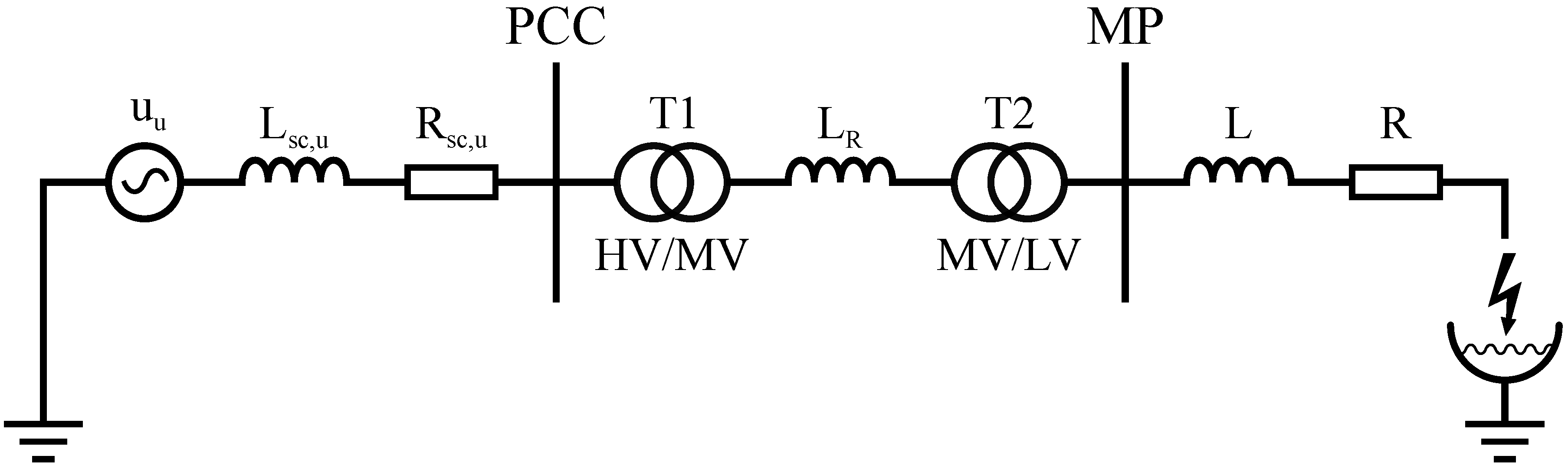
Figure 2.
Simplified equivalent circuit of the AC EAF system.
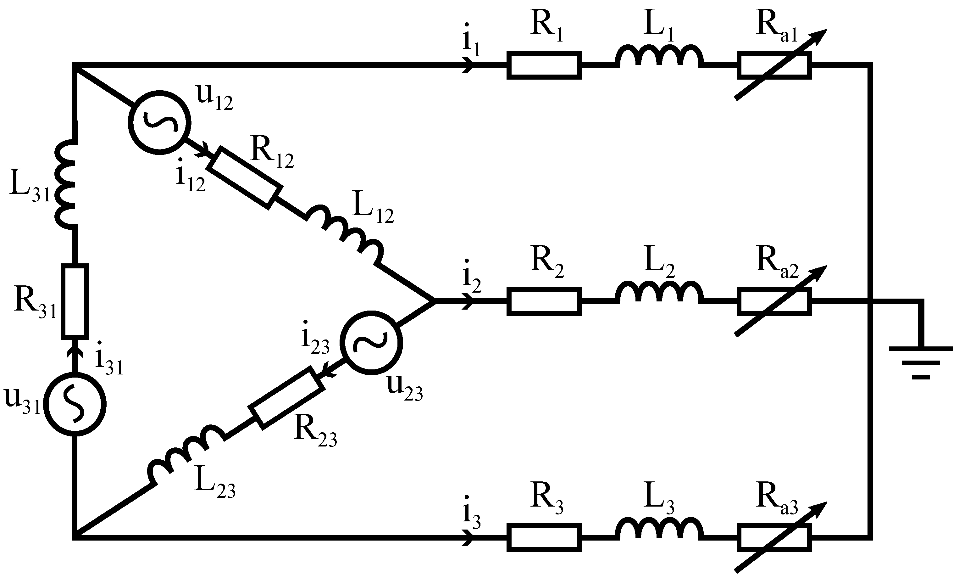
Figure 3.
Estimated arc length, derived from the effective arc voltage for all three lines.
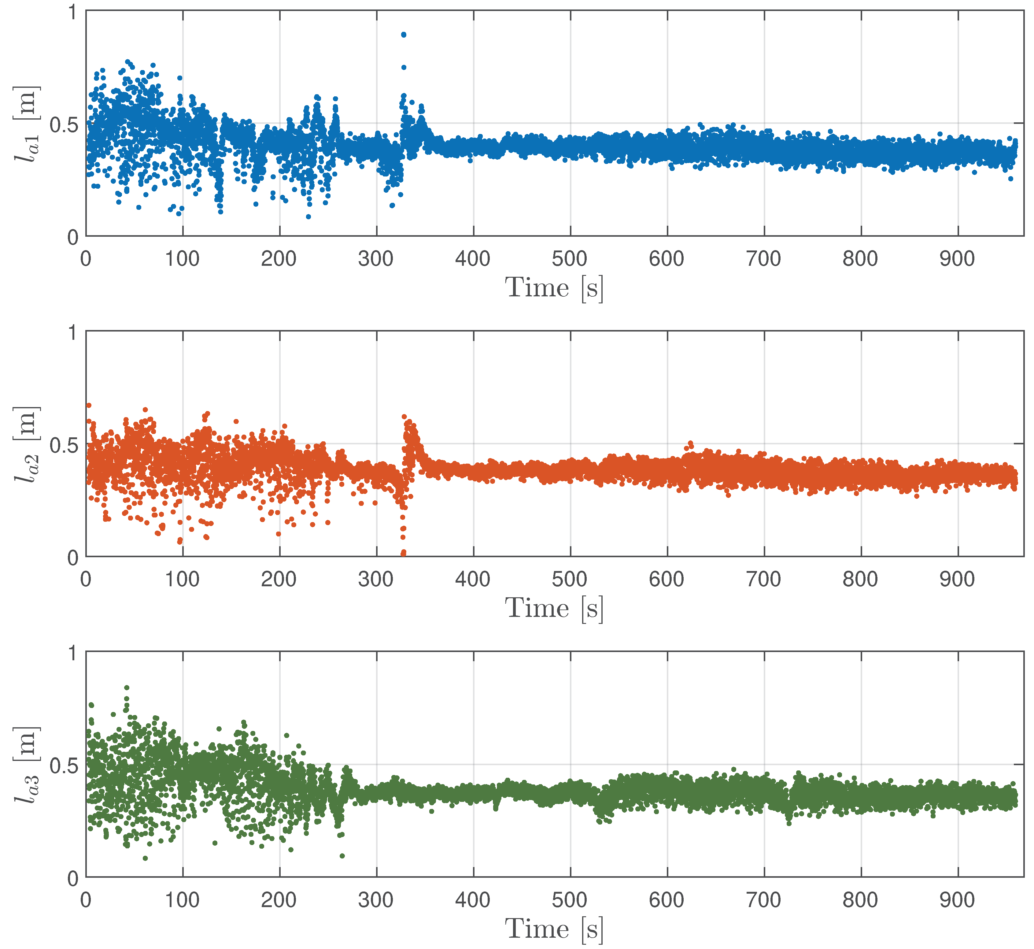
Figure 4.
Values of fitness function during the heat.
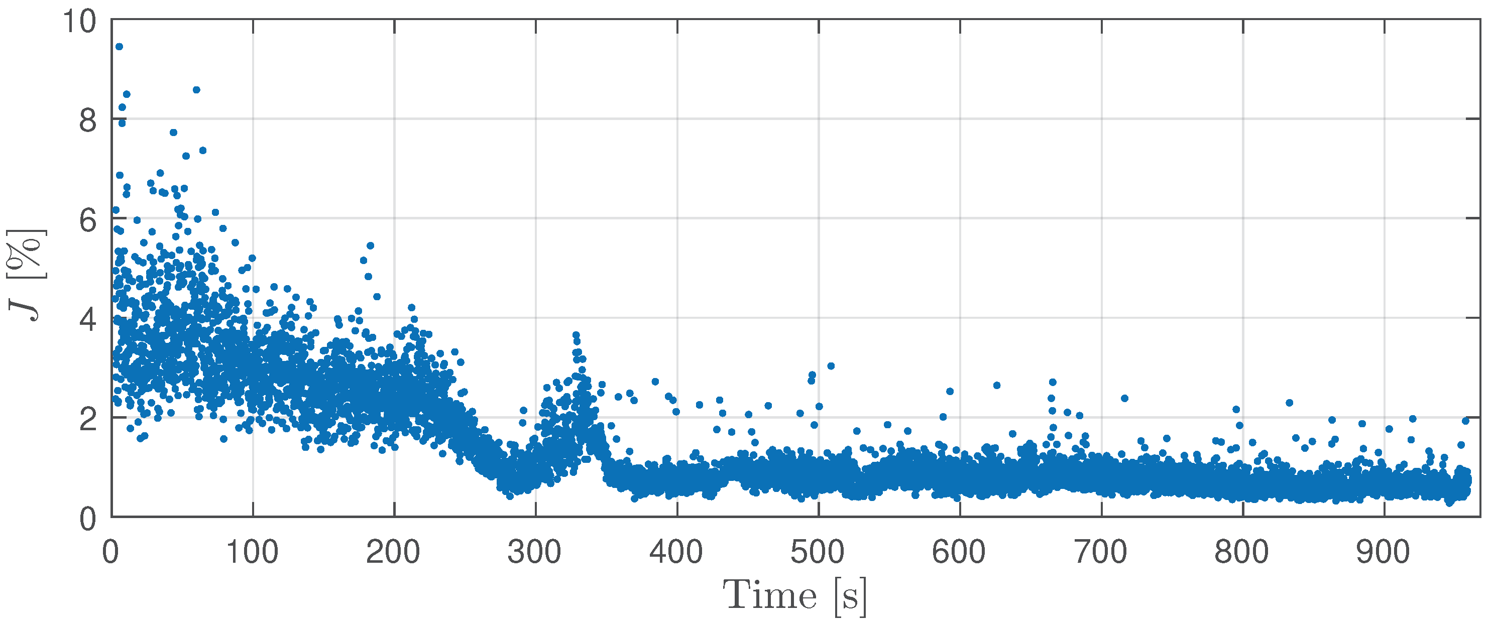
Figure 5.
Comparison of the simulated and measured line-to-ground voltage and line currents during the melting stage.
Figure 5.
Comparison of the simulated and measured line-to-ground voltage and line currents during the melting stage.
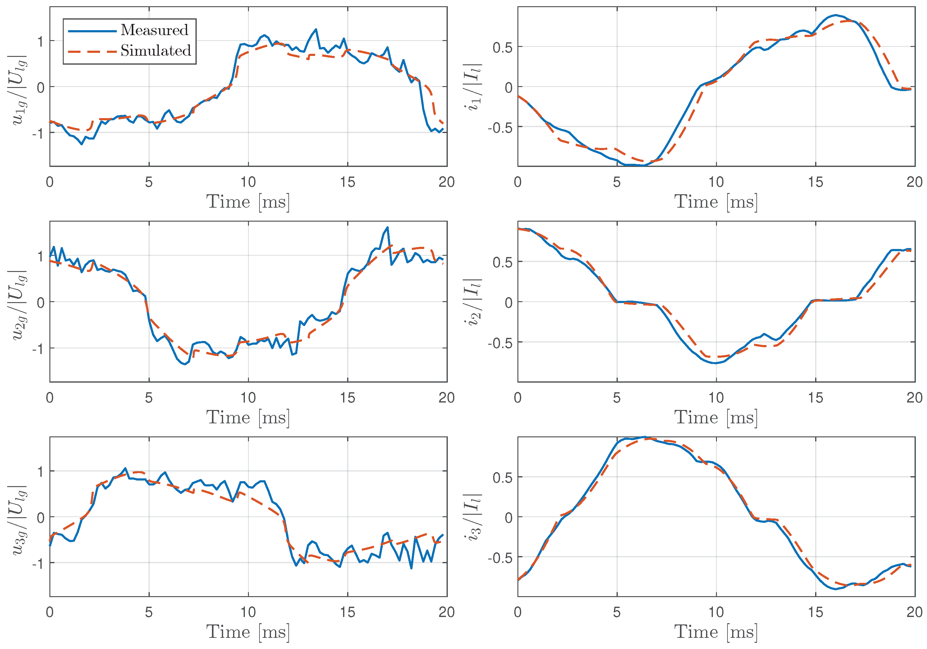
Figure 6.
Calculated arc resistance and binary state indicators for each line.
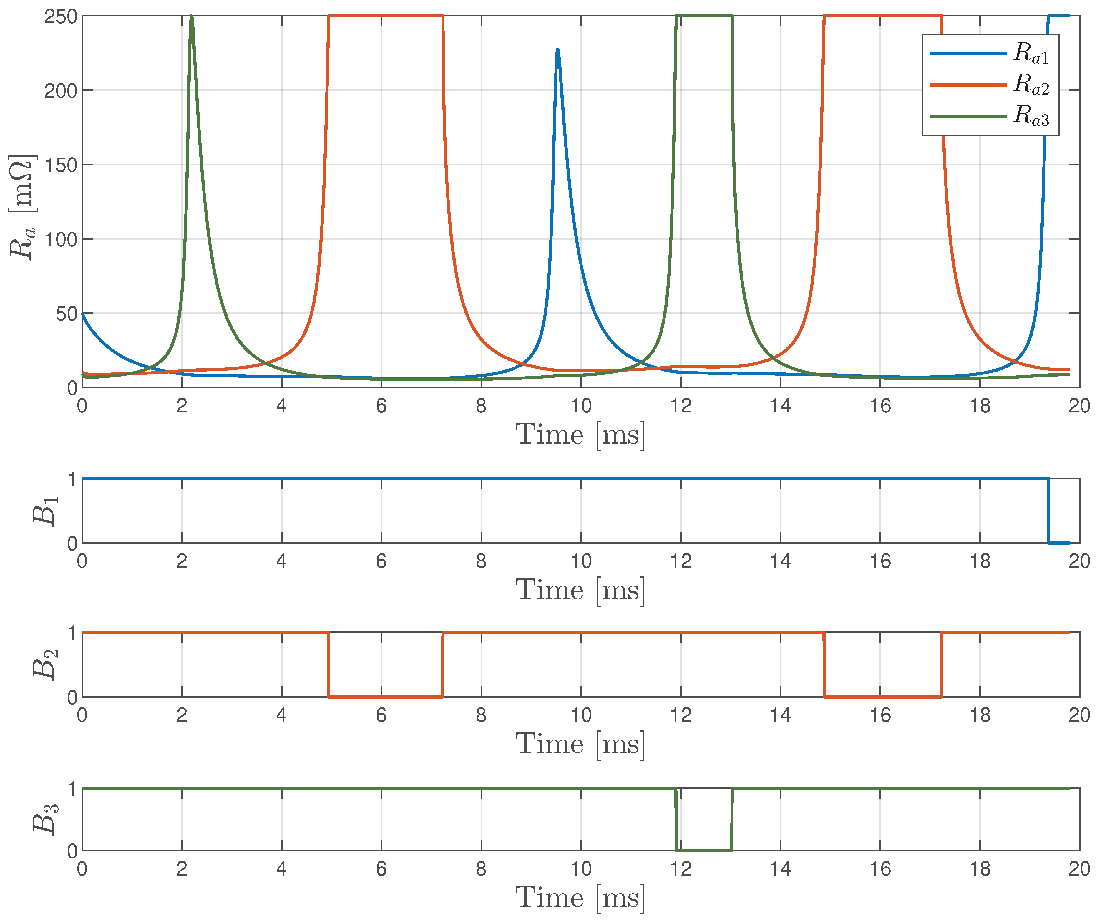
Figure 7.
Comparison of the simulated and measured line-to-ground voltage and line currents during the refining stage.
Figure 7.
Comparison of the simulated and measured line-to-ground voltage and line currents during the refining stage.
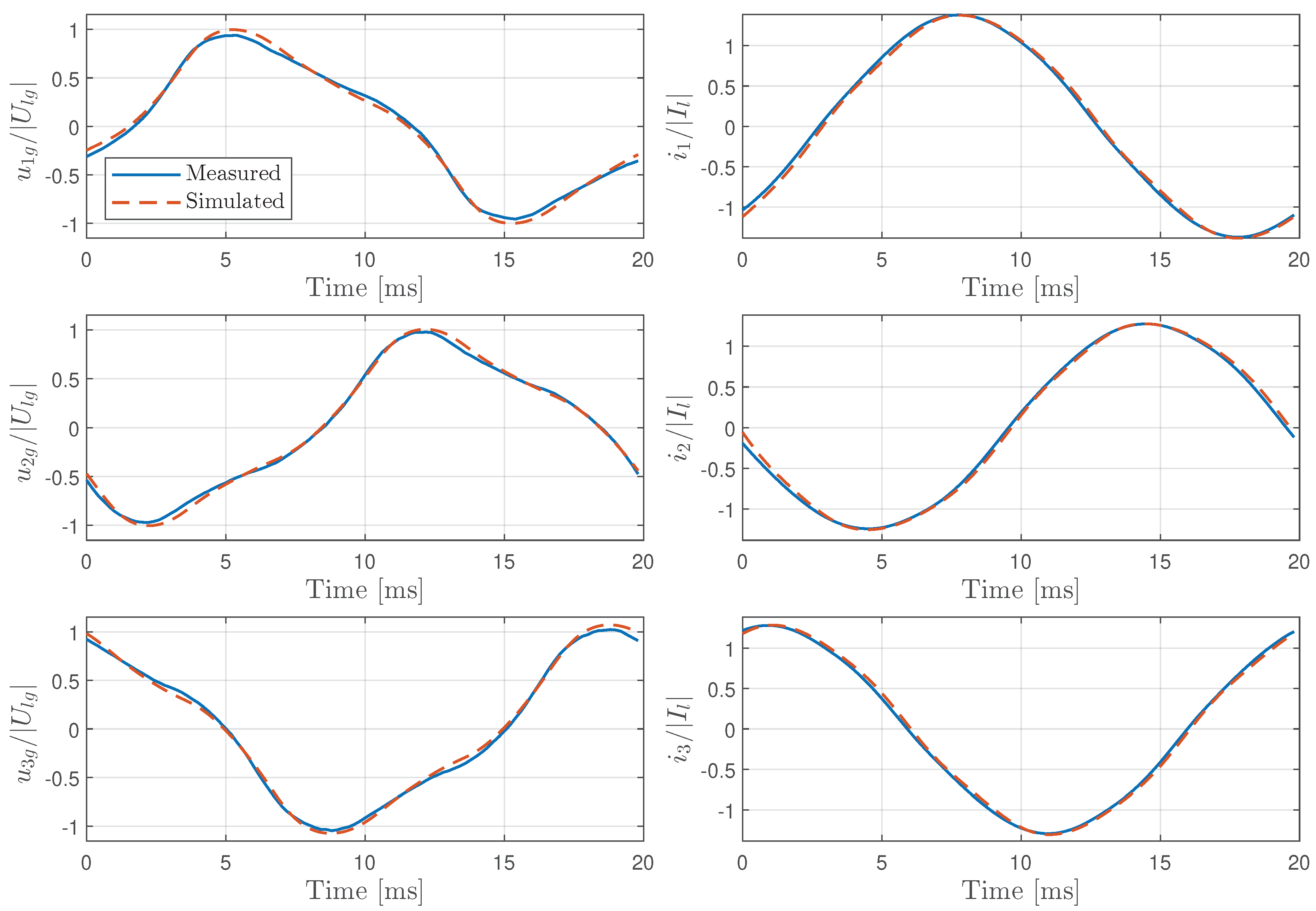
Figure 8.
Calculated arc resistance for all three lines during the refining stage.
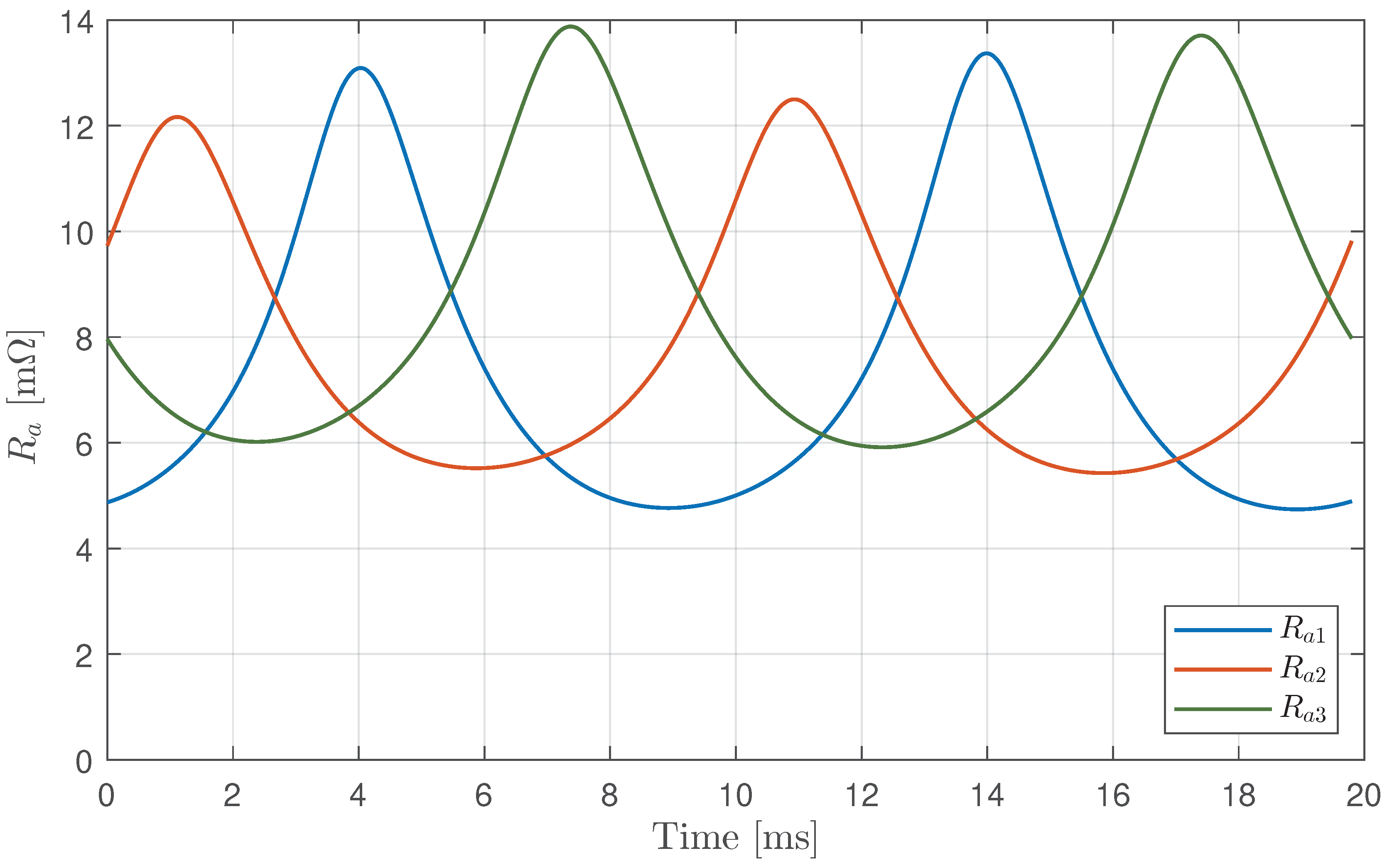
Figure 9.
The AQI calculated for all three lines illustrates the progression from the melting stage to the refining stage.
Figure 9.
The AQI calculated for all three lines illustrates the progression from the melting stage to the refining stage.
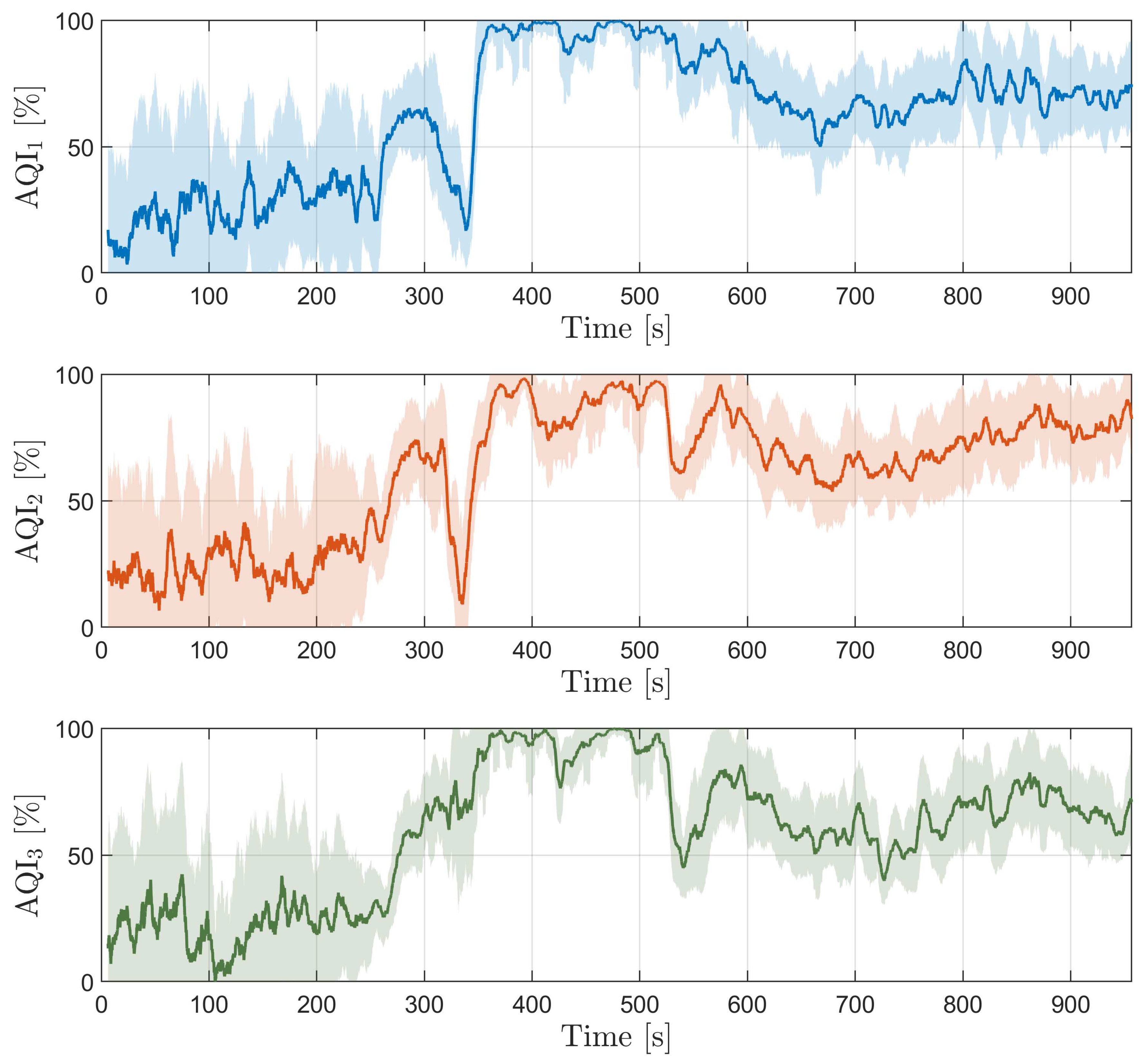

Table 1.
Mean values of the fitness function components for the entire dataset, melting stage and refining stage.
Table 1.
Mean values of the fitness function components for the entire dataset, melting stage and refining stage.
| Fitness [%] | All | Melting | Refining |
|---|---|---|---|
| 1.40 | 2.39 | 0.77 | |
| 1.97 | 3.19 | 1.19 | |
| 0.83 | 1.59 | 0.35 |
Disclaimer/Publisher’s Note: The statements, opinions and data contained in all publications are solely those of the individual author(s) and contributor(s) and not of MDPI and/or the editor(s). MDPI and/or the editor(s) disclaim responsibility for any injury to people or property resulting from any ideas, methods, instructions or products referred to in the content. |
© 2024 by the authors. Licensee MDPI, Basel, Switzerland. This article is an open access article distributed under the terms and conditions of the Creative Commons Attribution (CC BY) license (http://creativecommons.org/licenses/by/4.0/).
Copyright: This open access article is published under a Creative Commons CC BY 4.0 license, which permit the free download, distribution, and reuse, provided that the author and preprint are cited in any reuse.


