Submitted:
28 January 2024
Posted:
29 January 2024
You are already at the latest version
Abstract
The orbitofrontal cortex (OFC) area plays a critical role in human brain functions. However, susceptibility differences between paranasal sinuses and nasal cavity tissues often cause local field variations in the OFC during MRI, resulting in image distortions and signal loss. In this paper, we introduce a subject-friendly neck passive shim solution aimed at enhancing field homogeneity in the brain, specifically in the OFC region. Utilizing 3D gradient-echo pulse sequences, main magnetic field (B0) maps of four subjects’ brains were acquired at 4T MRI. Subsequently, these maps were decomposed into spherical harmonic coefficients and averaged. Optimal positions for placing shim elements on a semi-cylindrical surface, positioned slightly above the neck and below the chin, were computed. The findings indicate a substantial enhancement in B0 homogeneity, particularly within the OFC region, through the integration of this semi-cylindrical passive shim system in conjunction with first and second-order active shimming.
Keywords:
MRI
; 4T MRI
; Brain
; Orbito-frontal Cortex Imaging
; Magnetic Susceptibility
; Passive Shim Development
; Passive Shim Placement.
1. Introduction
The human brain is a complex and intricate organ responsible for a wide range of cognitive and physiological functions [1,2,3]. It comprises different lobes, with the frontal lobe being a crucial region associated with various higher cognitive processes, including decision-making, problem-solving, and social behavior [4,5,6,7]. Nestled within the ventral aspect of the frontal lobe resides the orbitofrontal cortex (OFC), a specialized sector of the prefrontal cortex [4,8]. Renowned for its pivotal role in cognitive processing and decision-making, the OFC is integral to human brain functions [9,10,11,12].
Magnetic Resonance Imaging (MRI) stands out as a highly auspicious neuroimaging technique employed in contemporary clinical environments [13,14]. It plays a pivotal tool in generating diagnostic medical images of the human brain, showcasing its vital role in accurately identifying pathological conditions in the central nervous system (CNS) [15,16,17,18]. However, susceptibility artifacts in MRI, arising from varying magnetic susceptibilities of adjacent tissues or substances, can cause distortions in images of the OFC. These artifacts manifest as signal voids or distortions in the generated images, potentially impacting the interpretation of tissue structures [19,20,21,22]. Common sources of susceptibility artifacts include air-tissue interfaces, metallic implants, and paramagnetic substances [20,23,24]. These variations in magnetic susceptibility result in local magnetic field inhomogeneities, causing image artifacts that can compromise the overall quality and diagnostic accuracy of MRI scans [23]. Understanding and mitigating susceptibility artifacts are crucial for ensuring the reliability and precision of MRI-based clinical assessments.
The significant variation in magnetic susceptibility between the ethmoid, frontal, and sphenoid sinuses and nasal cavities (air-filled cavities adjacent to the OFC) is attributed to susceptibility-induced imaging artifacts in the OFC [25]. Localized passive shimming, as evidenced by previous studies, reduces field deviations in the OFC. It’s beneficial to position shim elements away from the subject for comfort [26,27,28,29,30]. In this study, we propose using a passive shim element positioned beneath the subject’s chin to generate a specifically compensated passive shim field, localized to the OFC region.
2. Materials and Methods
The magnetic susceptibility variance between brain tissue, paranasal sinuses, and the nasal cavity results in significant local susceptibility-induced field variations specifically within the OFC. Previous efforts have focused on enhancing magnetic field homogeneity in key brain regions like the inferior frontal cortex (IFC) and inferior temporal cortex (ITC) [28,29,30]. The following section outlines the numerical analysis of the inhomogeneous magnetic field, along with the design and construction details of the localized neck-passive shim system.
The methodology involves deriving average amplitudes of spherical harmonics for local dipole passive shimming based on brain field maps (B) obtained from multiple subjects. This is followed by simulations and measurements to verify the potential of the local dipole passive shim system in enhancing field homogeneity within the OFC. The performance is evaluated through assessments of its corresponding full width and half maximums (FWHMs). Subsequently, the determination of required magnetic susceptibilities and dimensions is achieved based on the selected average amplitude strengths and positions.
2.1. Design of the Neck Passive Shim System
Figure 1 demonstrates spherical shim elements, comprising diamagnetic and/or para/ferromagnetic material and with radius (al) and susceptibility , placed on a half-cylindrical surface at predefined positions of a passive shim system within the main magnetic field (B0). These elements generate a magnetic induction () outside the surface at a given position (x, y, z), as shown in Equation 1 [31,32,33,34]. Here, the unit vector denotes the z-direction
Here, x, y, and z are Cartesian coordinates describing 3D space and l represents the number of shim pieces. The simplified version of Equation 1 is given below [26].
Here, and represent the spatial-dependent components and the amplitude of the induced passive shim field, respectively. Furthermore, the symbols of , , and the subscript of i, j, k represent the orientation and the matrix position of the Cartesian coordinates, respectively. The amplitude depends on the magnetic susceptibility and the dimensions of each individual shim insert. The least-squares optimal for the individual subjects are determined by Equation 3 below (where n’ is the number of subjects in the group).
Here, represents the measured frequency shift due to field inhomogeneity at voxel position , , and of the subject, and the -1 and T superscripts signify matrix inversion and transposition, respectively. The average amplitude of each spherical harmonic component is given by Equation 4 below:
2.2. Data Acquisition and Field Mapping
In this study, a 3D gradient-echo pulse sequence was employed. To acquire the magnetic field maps of each subject’s brain, these maps were projected onto a spherical harmonic model (as per Equation 1). This projection allowed for the extraction of the desired amplitudes of the induced passive shim field tailored for each subject. Subsequently, these amplitudes were averaged (as described in Equation 4) across all subjects to derive the final design. This averaging process ensured the incorporation of the overall characteristics of the induced passive shim field across multiple subjects for the ultimate system design.
2.3. Passive Shim System Design
For the fundamental geometry of the passive shim system, a semi-cylindrical shape was chosen. Its parameters included an outside diameter of 20.5 cm, inside diameter of 20.0 cm, and a length of 4 cm. The positions of the shim elements were thoroughly assessed and adapted to suit the requirements for the passive shim design. Upon finalizing the positions and the average values, this information was utilized to determine the necessary susceptibilities , dimensions, and corresponding masses required for the construction of the shim elements. This thorough evaluation and determination facilitated the precise development of the passive shim system for the intended application.
2.4. Magnetic Properties of the Passive Shim Insert
Following the computed magnetic susceptibilities, two distinct materials were employed to fabricate the localized dipole passive shim system. For this purpose, mu-metal (Ad-Vance Magnetics, Inc.), consisting of Ni (77%), Fe (16%), Cu (5%), and Cr (2%) by mass composition, was selected as the ferromagnetic material. Additionally, bismuth (Chemical Store, Main Avenue, New Jersey) was utilized as the diamagnetic material. The respective densities of mu-metal and bismuth are 8.75 g/cc and 9.78 g/cc. These material choices were made to best achieve the required magnetic properties essential for the construction of the dipole passive shim system.
2.5. Construction of Localized Dipole Passive Shim System
The assembly process began by affixing the combined ferromagnetic and diamagnetic passive shim inserts at designated positions on a paper sheet measuring 4.0 cm in length and 50.0 cm in width. These positions were precisely marked at intervals of 0, ±5, ±10, ±15, ±20 cm along the x-axis and 10.0, 10.5, 11.0, 11.5, 12.0, 12.5, 13.0, and 13.5 cm along the z-axis within the Cartesian coordinate system. Subsequently, the paper was meticulously wrapped around the exterior surface of the plastic semi-cylinder, which served as the base for the dipole passive shim system. Special attention was given to aligning the position of x = 0 with the vertical rod of the passive shim system, ensuring accurate alignment relative to the magnet’s iso-center. The optimal mounting position of the semi-cylindrical passive shim system was determined based on the y-z plane (sagittal plane). Upon completion, the passive shim system was securely attached to the radio frequency (RF) coil, maintaining alignment such that the y-z plane was in congruence with the movable vertical and horizontal rods of the dipole passive shim system, as illustrated in Figure 2.
2.6. Both Local Dipole Passive and Active Shimming In Vivo
The investigation encompassed an assessment of field distributions within the human brain under two distinct scenarios: the first involved solely active shimming utilizing Fast, automatic shimming by mapping along projections (FASTMAP) [34,35,36]. In contrast, the second scenario encompassed a combined approach integrating both active shimming and local dipole passive shimming. These assessments were conducted through a modified 3D gradient-echo pulse sequence deployed on the 4T scanner. In the comparison analysis, the variation in field strength within the OFC region was meticulously scrutinized and compared between the field maps generated solely through active shimming and those resulting from the amalgamation of local dipole passive and active shimming methodologies.
3. Results
3.1. Local Passive Shim Model for the Human OFC at 4T.
The evolution of magnetic field homogeneity within the human brain, particularly targeting the orbitofrontal cortex (OFC), is illustrated in Figure 3 subsequent to the incorporation of the localized dipole magnetic passive shim field alongside active shimming. The figure exhibits: (A) measured magnetic field maps of the brain following the active shimming; (B) simulated dipole magnetic field induced by a passive shim element; (C) simulated residual maps after optimization by the dipole passive shim positioned in the subject’s mouth; and (D) simulated residual maps after optimization by combining the active and the dipole passive shim (equivalent to C condition). Comparing the measured field map (Figure 3-A) with the simulated map optimized by both active and localized dipole passive shimming (Figure 3-D) demonstrates a notable improvement in field homogeneity within the brain, especially within the OFC. Figure 3-B indicates a relatively small dipole field, necessitating the shim piece’s proximity to the sinus region. However, placement of the shim piece within the subject’s mouth poses discomfort. To address this, we propose employing a dipole passive shim element positioned beneath the subject’s chin. This configuration induces a locally targeted dipole field aimed at compensating for the field inhomogeneity within the OFC. Figure 4 depicts the passive shim system comprising diamagnetic (green) and para/ferromagnetic (red) shim pieces designed to induce an effective dipole passive shim field.
The magnetic field distribution following active shimming (i.e. the first and second order) for each subject was projected into the spherical harmonic function (Equation 3, resulting in individual spherical harmonic amplitudes, . To finalize the shim set design, the average amplitudes were computed using Equation 4. Figure 5 illustrates the magnitudes and variations of the spherical harmonic coefficients for each subject, along with the average amplitudes across all subjects. Notably, harmonics whose values oscillate between positive and negative fields pose a challenge. Creating a magnetic field with positive amplitudes necessitates a paramagnetic or ferromagnetic material, whereas generating a negative field requires a diamagnetic element.
To determine the optimal mounting positions of the dipole passive shim geometry, Figure 6 displays the Full Width and Half Maximum (FWHM) of the brain field distribution as a function of the shim set within the y and z coordinates on the sagittal plane. The plot colorizes the regions based on field variation, where blue regions indicate successful shimming (i.e., smaller field variation) while red denotes inadequate shimming. As Figure 6 illustrates, the best mounting position along the y and z axis lies approximately 5.5 - 7.0 cm and 11.5 – 13.0 cm, respectively.
Figure 7 displays (A) the measured brain map for the third subject across axial, coronal, and sagittal planes following initial active shim, and (B) the optimized simulated maps resulting from the combined application of active and averaged local dipole passive shimming. The corresponding FWHM values representing the magnetic field variation across the entire brain volume for the subject are presented in Figure 8.
Comparing the uncorrected field map (Figure 7-A) with the simulated map (Figure 7-B) demonstrates a clear enhancement in the field homogeneity across the entire brain. Moreover, the optimized simulated field maps achieved through combined active and dipole shimming methods (Figure 7-B) show a notably greater improvement in field homogeneity, particularly within the OFC and frontal regions, compared to the active shimming alone (Figure 7-A). These simulation results underscore the potential effectiveness of the developed local dipole passive shim system in mitigating field inhomogeneity in the human brain, specifically within the OFC. Additionally, the FWHM of the field distribution after the initial active shimming consistently exceeds that of the simulated field map that incorporates at least one passive shim (Figure 8). After implementing optimal active shimming, the FWHM of the simulated field map (Figure 8-B) shows an approximate reduction of 42.3% for the third subject, mirroring similar trends observed for the first, second, and fourth subjects within the group. This trend in the simulation field maps (Figure 7) and the associated histograms (Figure 8) strongly suggests the potential of this technique in enhancing field homogeneity, especially within the OFC, across multiple subjects.
3.2. The Local Dipole Passive Shim Field on the Phantom at 4T.
Diamagnetic (bismuth) and ferromagnetic (mu-metal) passive shim pieces were used to generate the local dipole field. A total of seven bismuth shim pieces with volumes of 0.2 cm3 (3 pieces), 0.5 cm3 (2 pieces), 1.0cm3 (1 piece), and 2.0 cm3 (1 piece), as well as ten mu-metal pieces with volumes of 0.00002 cm3 (2 pieces), 0.0001 cm3 (2 pieces), 0.0003 cm3 (2 pieces), 0.003 cm3 (3 pieces), and 0.007 cm3 (1 piece) were strategically positioned on the surface of the half-cylindrical (Figure 4). The experimental generation of the localized dipole magnetic field within the phantom was examined across the axial, coronal, and sagittal planes (illustrated in Figure 9). Observations of the dipole passive shim field maps within the phantom, especially in the axial and sagittal planes, depict the successful generation of the desired dipole field by the passive shim system.
3.3. The Local Dipole Passive and Active Shimming on the Human Brain at 4T.
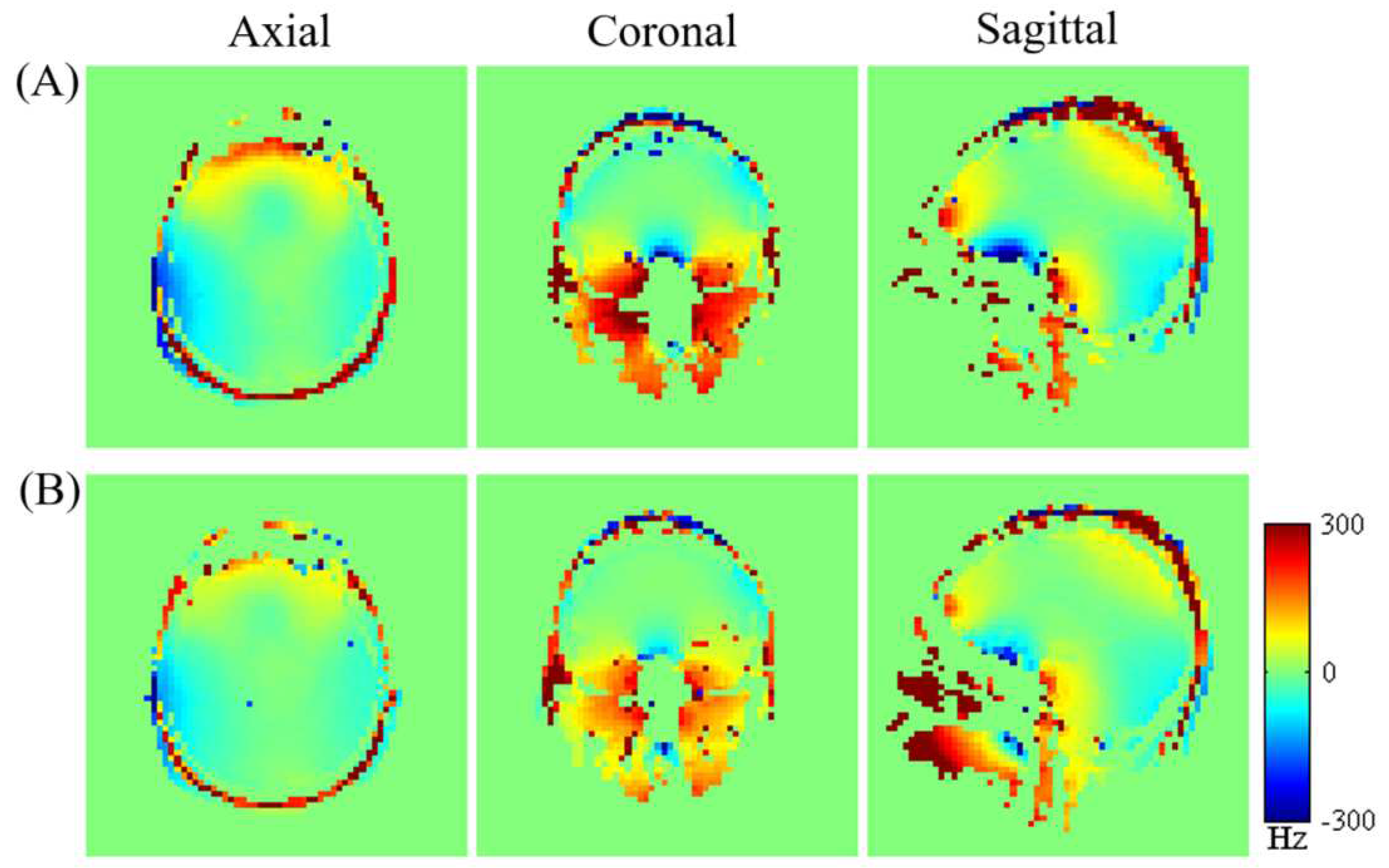
The enhancement of the magnetic field homogeneity within the human brain, following the introduction of the averaged local dipole passive shim field along with the active shimming, is depicted in Figure 10. The measured magnetic field distributions within the brain after (A) active shimming alone and (B) combined active and local dipole passive shimming are demonstrated in Figure 10. In Figure 10-A, residual inhomogeneity is observed in several brain regions even after active shimming, notably in the frontal lobe, orbitofrontal cortex (OFC), parietal lobe, temporal lobe, upper cerebellum, and sinus areas. Nevertheless, upon the addition of localized dipole passive shimming, an improvement in field homogeneity is evident across various brain regions, particularly those closer to the ethmoid and sphenoid sinuses and the parietal lobe (Figure 10-B). Additionally, a subtle improvement in the homogeneity within the frontal lobe is observed, as noticeable in the sagittal and axial field maps depicted in Figure 10-A and Figure 10-B.
4. Discussion and Conclusion
Despite the adequacy of first- and second-order active shimming in some regions of the human brain, our simulations reveal persistent limitations in improving field homogeneity across all areas. Combining active shimming with averaged local dipole shimming appears to mitigate this limitation. While our results demonstrate that existing active shimming can improve field homogeneity in certain brain areas, challenges persist in regions proximal to sinuses. However, our simulations and experimental data exhibit that the inclusion of a local dipole passive shim effectively overcomes these challenges, particularly in enhancing field homogeneity over sinus regions, as seen in our simulated field maps (Figure 3).
The efficacy of the induced localized dipole passive shim field is proportional to . Therefore, the distance between passive shim inserts and the target shimming area should be short to be effective. The proposed half-cylindrical passive shim system is placed below the chin, which is relative remote to the OFC region. Due to the relatively long distance between the OFC and shim inserts, the required amount and magnitude of the magnetic susceptibility of passive shim inserts are considerably large in our design. In addition, to generate a strong dipole field, it is essential to use shim material with highly negative magnetic susceptibility that is usually unavailable in nature, or to use a large quantity of shim elements that may be limited by the dimension of the design.
Placement of the dipole passive shim system, specifically below the chin and slightly above the neck, supported by a half-cylindrical geometry, may face challenges for subjects with varying neck sizes or due to geometric limitations of the shim system. Consequently, this approach might not universally accommodate all subjects.
5. Conclusions
Employing a local dipole passive shim field holds promise for enhancing field homogeneity within localized brain regions. This study underscores the accuracy in placing appropriate diamagnetic and ferromagnetic materials on the half-cylinder’s surface to generate a localized dipole, effectively mitigating inhomogeneity in the OFC. Notably, this technique is operator and subject-friendly. Equations 3 and 4 provide crucial tools to determine magnetic susceptibility and dimensions for optimizing field homogeneity. However, incorrect estimations of these factors may potentially compromise the final outcome.
Author Contributions
Conceptualization, Jing-Huei Lee, Mohan L. Jayatilake and Sahan M. Vijithananda; methodology, Jing-Huei Lee, Mohan L. Jayatilake; software, Mohan L. Jayatilake; validation, Jing-Huei Lee, Mohan L. Jayatilake and Sahan M. Vijithananda; formal analysis, Mohan L. Jayatilake, Sahan M. Vijithananda; investigation, Jing-Huei Lee, Mohan L. Jayatilake; resources, Jing-Huei Lee, Mohan L. Jayatilake; data curation, Mohan L, Jayatilake; writing—original draft preparation, Mohan L. Jayatilake and Sahan M. Vijithananda; writing—review and editing, Jing-Huei Lee, Mohan L. Jayatilake and Sahan M. Vijithananda; visualization, Mohan L. Jayatilake, Sahan M. Vijithananda .; supervision, Jing-Huei Lee; project administration, Jing-Huei Lee; funding acquisition, Not applicablel authors have read and agreed to the published version of the manuscript.
Funding
This research received no external funding.
Institutional Review Board Statement
Not Applicable. Justification: The decision to forgo seeking ethical clearance for the study titled "Development and Optimization of a Novel Passive Shim System for Human Orbitofrontal Cortex Imaging at 4T MRI" is grounded in the fundamental nature of the research. The study, centering on mathematical calculations, MRI physics, and simulation models, is devoid of direct involvement with human/animal subjects. As the research exclusively relies on theoretical and simulation-based approaches, there is no interaction with patients or collection of human data, mitigating the necessity for ethical clearance. Additionally, the development of the passive shim system does not incorporate any human-specific data, further alleviating ethical concerns related to the study. This decision is underscored by the absence of experimental procedures impacting human subjects and the overall focus on theoretical and simulation-based methodologies, which collectively contribute to a research framework that does not warrant ethical clearance. It is imperative to clearly communicate these factors in any relevant documentation or communication to ensure transparency and understanding among stakeholders.
Informed Consent Statement
Informed consent was obtained from the three volunteers who volunteered to visualize the effect of the developed passive shim system.
Data Availability Statement
Not Applicable.
Acknowledgments
I express heartfelt gratitude to Judd Storrs and Jeff Osterhage from the Center for Imaging Research, University of Cincinnati, Cincinnati, OH, United States, for their indispensable support, instrumental in the success of this research. Their guidance and unwavering commitment significantly contributed to achieving research goals.
Conflicts of Interest
The authors declare that they have no conflict of interests.
Abbreviations
The following abbreviations are used in this manuscript:
| OFC | The orbitofrontal cortex |
| MRI | Magnetic Resonance Imaging |
| 4T | 4 Tesla |
| IFC | Inferior Frontal Cortex |
| ITC | Inferior Temporal Cortex |
| FASTMAP | Fast, Automatic Shimming by Mapping Along Projections |
| FWHM | Full Width and Half Maximum |
References
- McEwen, B.S. Physiology and neurobiology of stress and adaptation: central role of the brain. Physiological reviews 2007, 87, 873–904. [Google Scholar] [CrossRef]
- Maldonado, K.A.; Alsayouri, K. Physiology, Brain 2019.
- Gabrieli, J.D. Cognitive neuroscience of human memory. Annual review of psychology 1998, 49, 87–115. [Google Scholar] [CrossRef]
- Stuss, D.T.; Knight, R.T. Principles of frontal lobe function; Oxford University Press, USA, 2013.
- Catani, M. The anatomy of the human frontal lobe. Handbook of clinical neurology 2019, 163, 95–122. [Google Scholar] [CrossRef]
- Alvarez, J.A.; Emory, E. Executive function and the frontal lobes: a meta-analytic review. Neuropsychology review 2006, 16, 17–42. [Google Scholar] [CrossRef]
- Fuster, J.M. Frontal lobe and cognitive development. Journal of neurocytology 2002, 31, 373–385. [Google Scholar] [CrossRef] [PubMed]
- Rolls, E.T.; Grabenhorst, F. The orbitofrontal cortex and beyond: from affect to decision-making. Progress in neurobiology 2008, 86, 216–244. [Google Scholar] [CrossRef] [PubMed]
- Stalnaker, T.A.; Cooch, N.K.; Schoenbaum, G. What the orbitofrontal cortex does not do. Nature neuroscience 2015, 18, 620–627. [Google Scholar] [CrossRef]
- Rolls, E.T. The orbitofrontal cortex and reward. Cerebral cortex 2000, 10, 284–294. [Google Scholar] [CrossRef] [PubMed]
- Rolls, E.T. Emotion, motivation, decision-making, the orbitofrontal cortex, anterior cingulate cortex, and the amygdala. Brain Structure and Function 2023, 1–57. [Google Scholar] [CrossRef] [PubMed]
- Rudebeck, P.H.; Rich, E.L. Orbitofrontal cortex. Current Biology 2018, 28, R1083–R1088. [Google Scholar] [CrossRef] [PubMed]
- Vijithananda, S.M.; Jayatilake, M.L.; Gonçalves, T.C.; Rato, L.M.; Weerakoon, B.S.; Kalupahana, T.D.; Silva, A.D.; Dissanayake, K.; Hewavithana, P. Texture feature analysis of MRI-ADC images to differentiate glioma grades using machine learning techniques. Scientific Reports 2023, 13, 15772. [Google Scholar] [CrossRef]
- Acampora, A.; Manzo, G.; Fenza, G.; Busto, G.; Serino, A.; Manto, A.; et al. High b-value diffusion MRI to differentiate recurrent tumors from posttreatment changes in head and neck squamous cell carcinoma: a single center prospective study. BioMed Research International 2016, 2016. [Google Scholar] [CrossRef] [PubMed]
- Thomas, M.A.; Hazany, S.; Ellingson, B.M.; Hu, P.; Nguyen, K.L. Pathophysiology, classification, and MRI parallels in microvascular disease of the heart and brain. Microcirculation 2020, 27, e12648. [Google Scholar] [CrossRef] [PubMed]
- Chen, J.J. Functional MRI of brain physiology in aging and neurodegenerative diseases. Neuroimage 2019, 187, 209–225. [Google Scholar] [CrossRef]
- Vijithananda, S.M.; Jayatilake, M.L.; Hewavithana, B.; Gonçalves, T.; Rato, L.M.; Weerakoon, B.S.; Kalupahana, T.D.; Silva, A.D.; Dissanayake, K.D. Feature extraction from MRI ADC images for brain tumor classification using machine learning techniques. Biomedical engineering online 2022, 21, 52. [Google Scholar] [CrossRef] [PubMed]
- Wardlaw, J.M.; Benveniste, H.; Nedergaard, M.; Zlokovic, B.V.; Mestre, H.; Lee, H.; Doubal, F.N.; Brown, R.; Ramirez, J.; MacIntosh, B.J.; et al. Perivascular spaces in the brain: anatomy, physiology and pathology. Nature Reviews Neurology 2020, 16, 137–153. [Google Scholar] [CrossRef] [PubMed]
- McKinstry III, R.C.; Jarrett, D.Y. Magnetic susceptibility artifacts on MRI: a hairy situation. American Journal of Roentgenology 2004, 182, 532–532. [Google Scholar] [CrossRef] [PubMed]
- Saritas, E.U.; Holdsworth, S.J.; Bammer, R. Susceptibility artifacts. Quantitative MRI of the spinal cord 2014, 91–105. [Google Scholar] [CrossRef]
- Shmueli, K.; de Zwart, J.A.; van Gelderen, P.; Li, T.Q.; Dodd, S.J.; Duyn, J.H. Magnetic susceptibility mapping of brain tissue in vivo using MRI phase data. Magnetic Resonance in Medicine: An Official Journal of the International Society for Magnetic Resonance in Medicine 2009, 62, 1510–1522. [Google Scholar] [CrossRef]
- Farahani, K.; Sinha, U.; Sinha, S.; Chiu, L.C.; Lufkin, R.B. Effect of field strength on susceptibility artifacts in magnetic resonance imaging. Computerized Medical Imaging and Graphics 1990, 14, 409–413. [Google Scholar] [CrossRef]
- Manson, E.N.; Inkoom, S.; Mumuni, A.N. Impact of magnetic field inhomogeneity on the quality of magnetic resonance images and compensation techniques: a review. Reports in Medical Imaging 2022, 43–56. [Google Scholar] [CrossRef]
- Cooper, J.J.; Young, B.D.; Hoffman, A.; Bratton, G.; Hicks, D.G.; Tidwell, A.; Levine, J.M. Intracranial magnetic resonance imaging artifacts and pseudolesions in dogs and cats. Veterinary Radiology & Ultrasound 2010, 51, 587–595. [Google Scholar] [CrossRef]
- Maroldi, R.; Ravanelli, M.; Borghesi, A.; Farina, D. Paranasal sinus imaging. European journal of radiology 2008, 66, 372–386. [Google Scholar] [CrossRef]
- Jayatilake, M.; Storrs, J.; Lee, J.H. A novel localized passive shim technique for optimizing magnetic field of the human orbitofrontal cortex at high field. Proc. Intl. Soc. Mag. Reson. Med 2010, 18, 1541. [Google Scholar]
- Schenck, J.F. The role of magnetic susceptibility in magnetic resonance imaging: MRI magnetic compatibility of the first and second kinds. Medical physics 1996, 23, 815–850. [Google Scholar] [CrossRef]
- Koch, K.M.; Brown, P.B.; Rothman, D.L.; de Graaf, R.A. Sample-specific diamagnetic and paramagnetic passive shimming. Journal of magnetic resonance 2006, 182, 66–74. [Google Scholar] [CrossRef] [PubMed]
- Hsu, J.J.; Glover, G.H. Mitigation of susceptibility-induced signal loss in neuroimaging using localized shim coils. Magn. Reson. Med 2005, 53, 243–248. [Google Scholar] [CrossRef]
- Wilson, J.L.; Jenkinson, M.; Jezzard, P. Protocol to determine the optimal intraoral passive shim for minimisation of susceptibility artifact in human inferior frontal cortex. Neuroimage 2003, 19, 1802–1811. [Google Scholar] [CrossRef]
- Boer, V.O.; Pedersen, J.O.; Arango, N.; Kuang, I.; Stockmann, J.; Petersen, E.T. Improving brain B0 shimming using an easy and accessible multi-coil shim array at ultra-high field. Magnetic Resonance Materials in Physics, Biology and Medicine 2022, 35, 943–951. [Google Scholar] [CrossRef]
- Zhang, X.; Zeng, L.; Zhang, H.; Huang, S. Magnetization model and detection mechanism of a microparticle in a harmonic magnetic field. IEEE/ASME Transactions on Mechatronics 2019, 24, 1882–1892. [Google Scholar] [CrossRef]
- Jenkinson, M.; Wilson, J.L.; Jezzard, P. Perturbation method for magnetic field calculations of nonconductive objects. Magnetic Resonance in Medicine: An Official Journal of the International Society for Magnetic Resonance in Medicine 2004, 52, 471–477. [Google Scholar] [CrossRef]
- Schwerter, M.; Hetherington, H.; Moon, C.H.; Pan, J.; Felder, J.; Tellmann, L.; Shah, N.J. Interslice current change constrained B0 shim optimization for accurate high-order dynamic shim updating with strongly reduced eddy currents. Magnetic resonance in medicine 2019, 82, 263–275. [Google Scholar] [CrossRef] [PubMed]
- Landheer, K.; Juchem, C. FAMASITO: FASTMAP Shim Tool towards user-friendly single-step B0 homogenization. NMR in Biomedicine 2021, 34, e4486. [Google Scholar] [CrossRef] [PubMed]
- Jayatilake, M.; Sica, C.T.; Elyan, R.; Karunanayaka, P. Comparison of FASTMAP and B0 Field Map Shimming at 4T: Magnetic Field Mapping Using a Gradient-Echo Pulse Sequence. Journal of Electromagnetic Analysis and Applications 2020, 12, 115–130. [Google Scholar] [CrossRef]
Figure 1.
Spherical shim elements placed at point on a half-cylindrical surface that induces the dipole passive shim field at position .
Figure 1.
Spherical shim elements placed at point on a half-cylindrical surface that induces the dipole passive shim field at position .
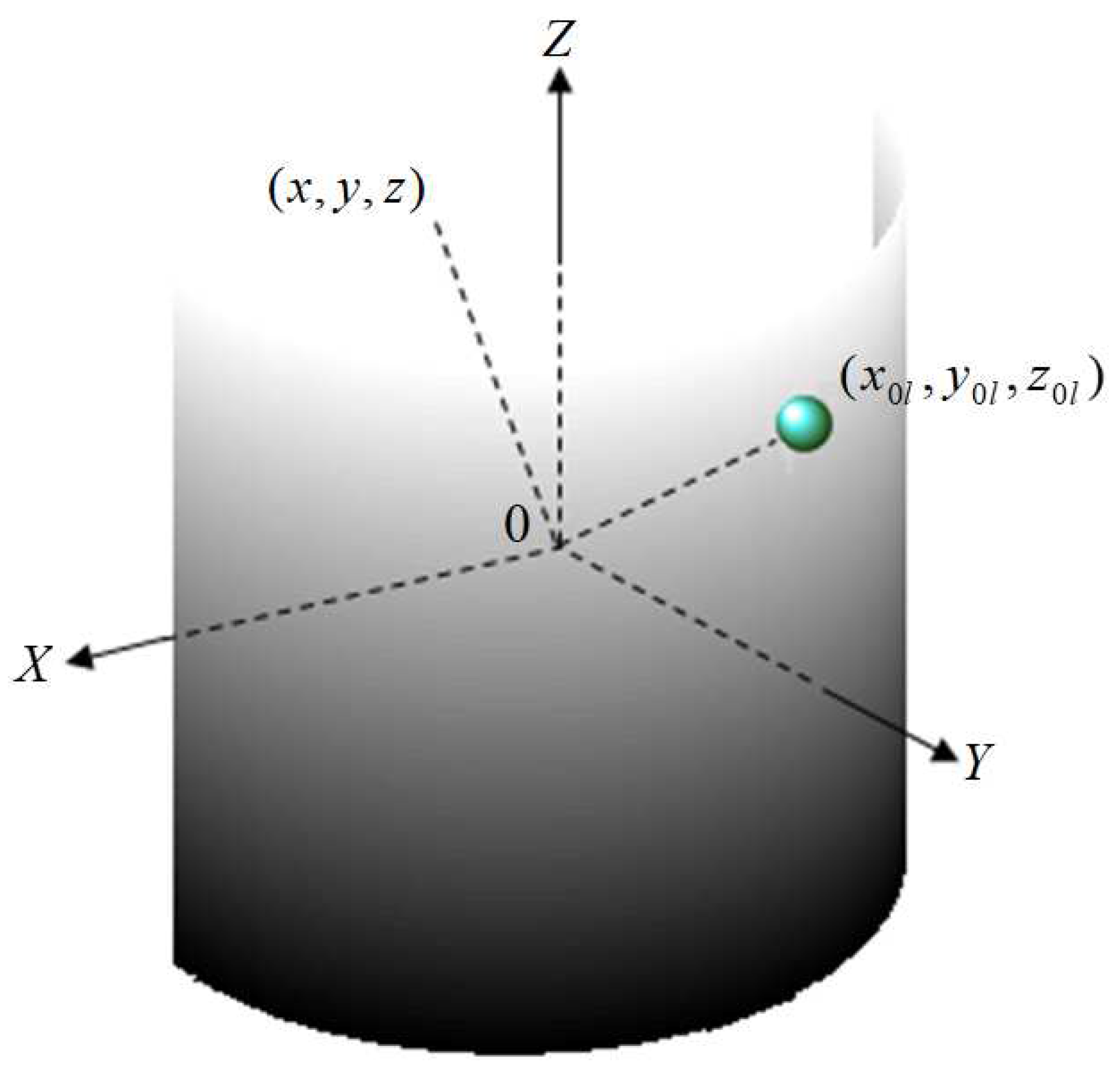
Figure 2.
A subject-friendly passive shim system positioned onto the RF coil.
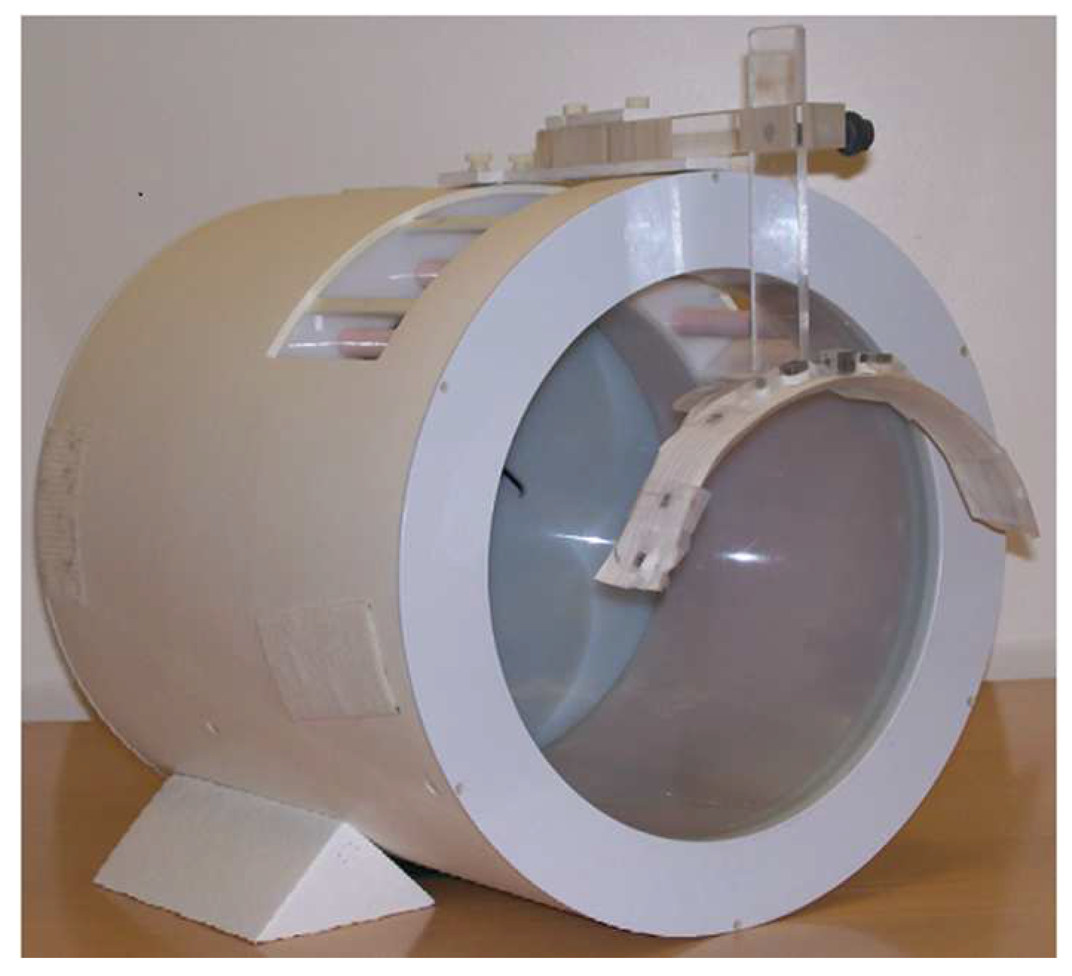
Figure 3.
The measured and simulated map of a human brain at 4T MRI. (A) The measured map for the axial, coronal, and sagittal slices of the 2nd subject’s brain with first- and second-order active shim. (B) A dipole magnetic induced by a magnetic passive shim element. (C) Simulated residual map optimized by a local dipole passive shim element inside the subject’s mouth. (D) Simulated residual map optimized by the first and second-order active shim as well as the localized dipole passive shim element inside the subject’s mouth.
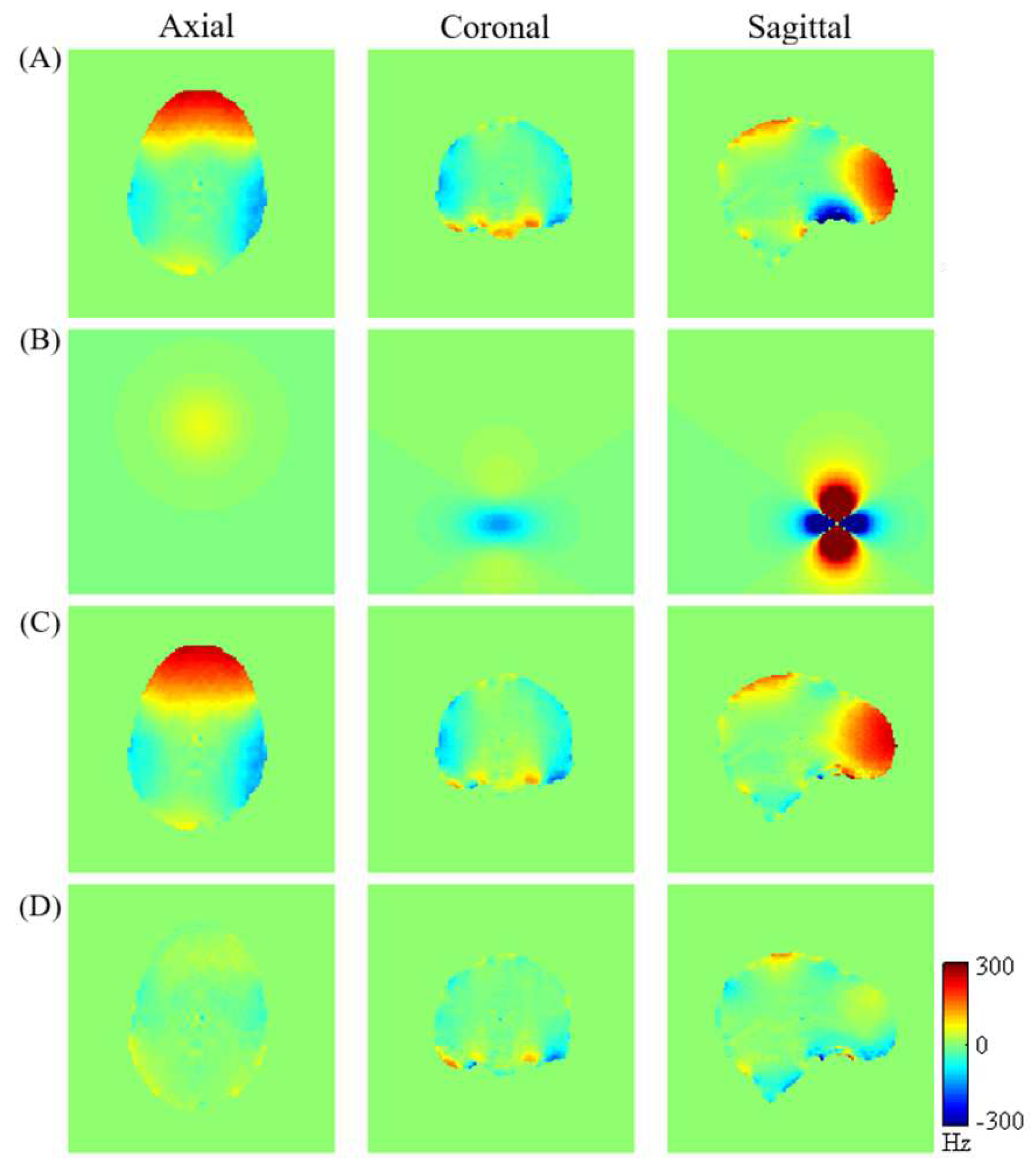
Figure 4.
Subject-friendly the passive shim system to be placed below the chin with predefined positions at a half-cylindrical geometry support. The colors green and red represent diamagnetic and para-/ferro-magnetic materials, respectively.
Figure 4.
Subject-friendly the passive shim system to be placed below the chin with predefined positions at a half-cylindrical geometry support. The colors green and red represent diamagnetic and para-/ferro-magnetic materials, respectively.
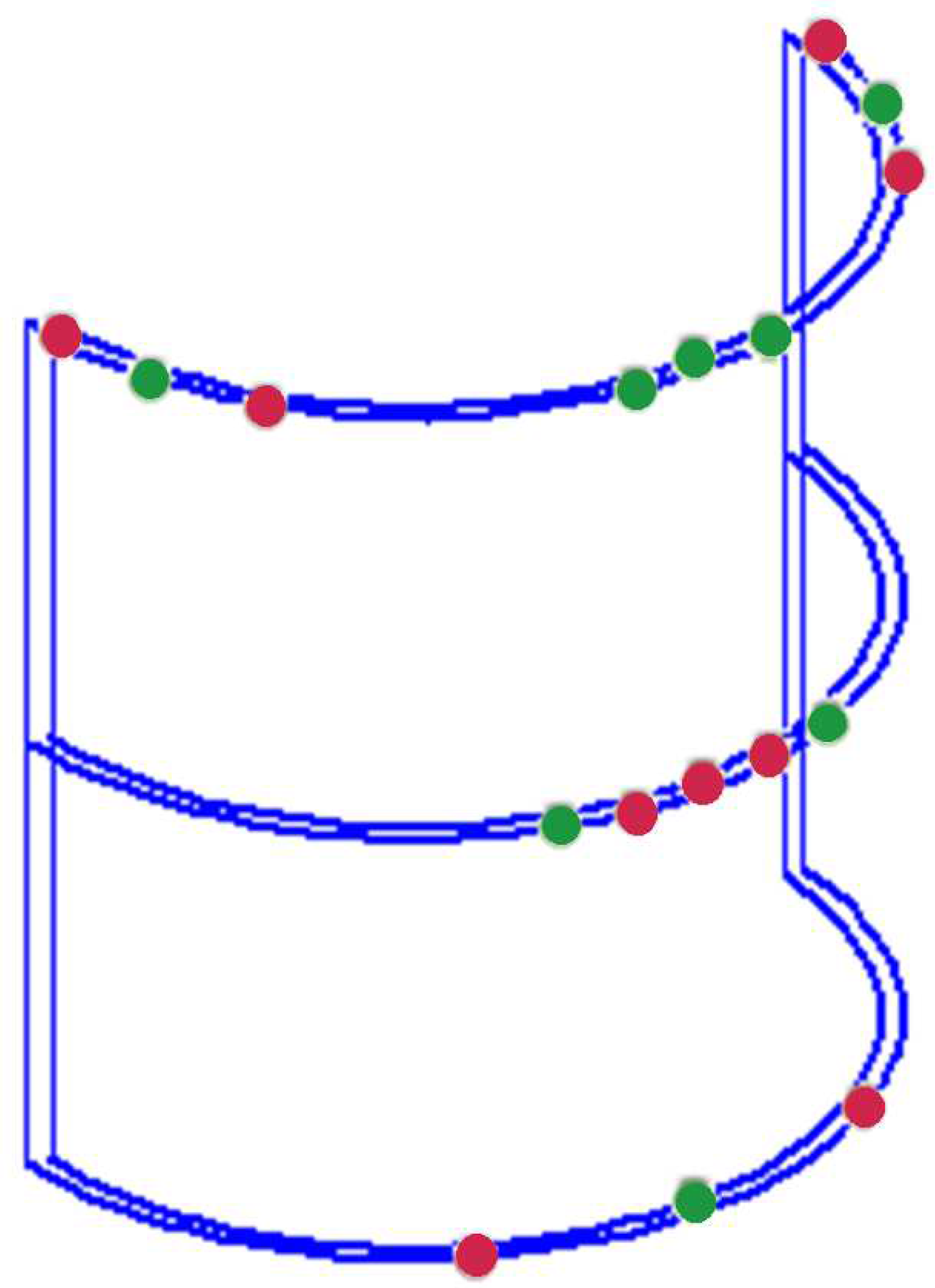
Figure 5.
Amplitudes of the spherical harmonic coefficients computed by Equation 3 for the first, second, third, and fourth subjects as well as the average amplitudes of all subjects.
Figure 5.
Amplitudes of the spherical harmonic coefficients computed by Equation 3 for the first, second, third, and fourth subjects as well as the average amplitudes of all subjects.
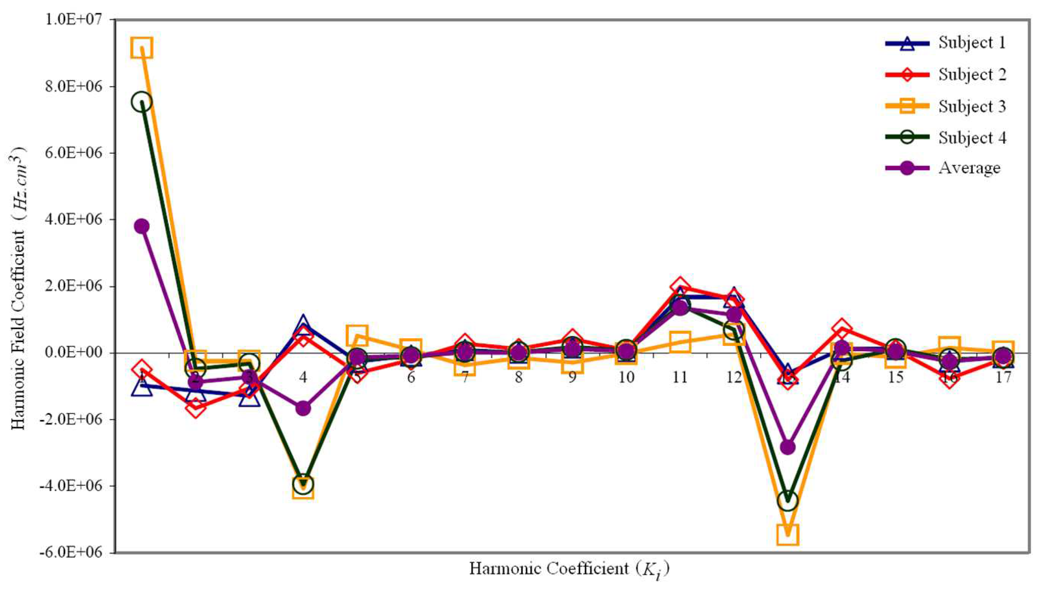
Figure 6.
Determination of best mounting positions of the half-cylindrical geometry (i.e. the dipole passive shim geometry) position in the sagittal plane. Blue indicates a more effective shimming. Plot of the FWHM of the field distribution of the third subject’s brain based on the y and z position of the half-cylindrical passive shim system.
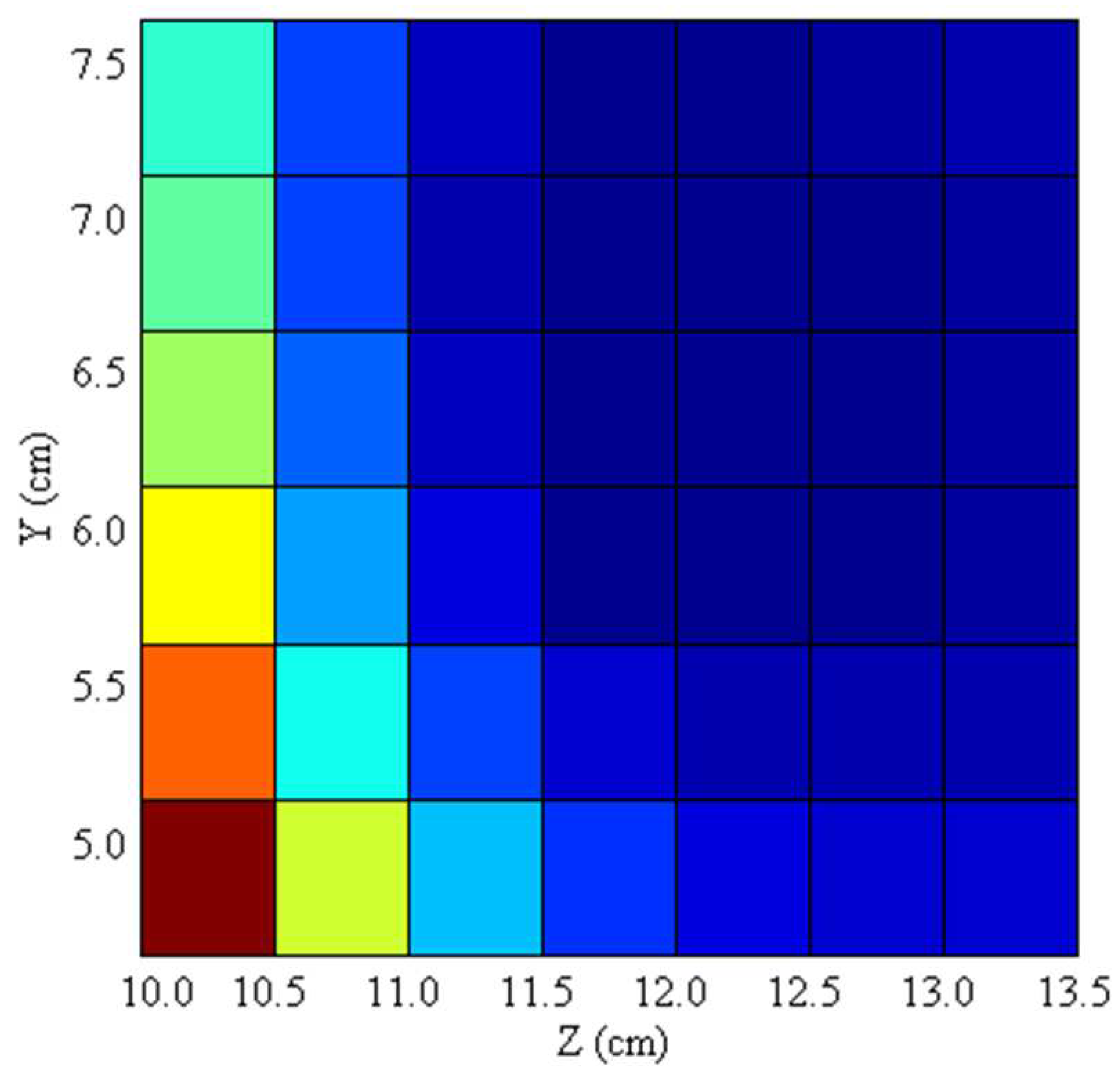
Figure 7.
Comparison of measured and predicted magnetic field map of the third subject’s brain. (A) map of the subject’s brain following an initial active shimming. (B) The predicted maps of the third subject optimized by the first- and second-order active shimming and the local dipole passive shimming.
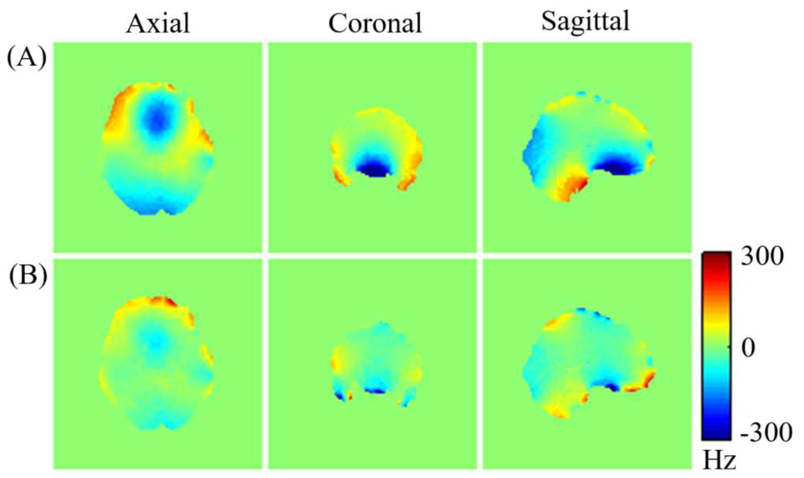
Figure 8.
Histograms of magnetic field distribution within the brains of the third subject corresponding to Figures 7 (A) and (B), respectively.
Figure 8.
Histograms of magnetic field distribution within the brains of the third subject corresponding to Figures 7 (A) and (B), respectively.
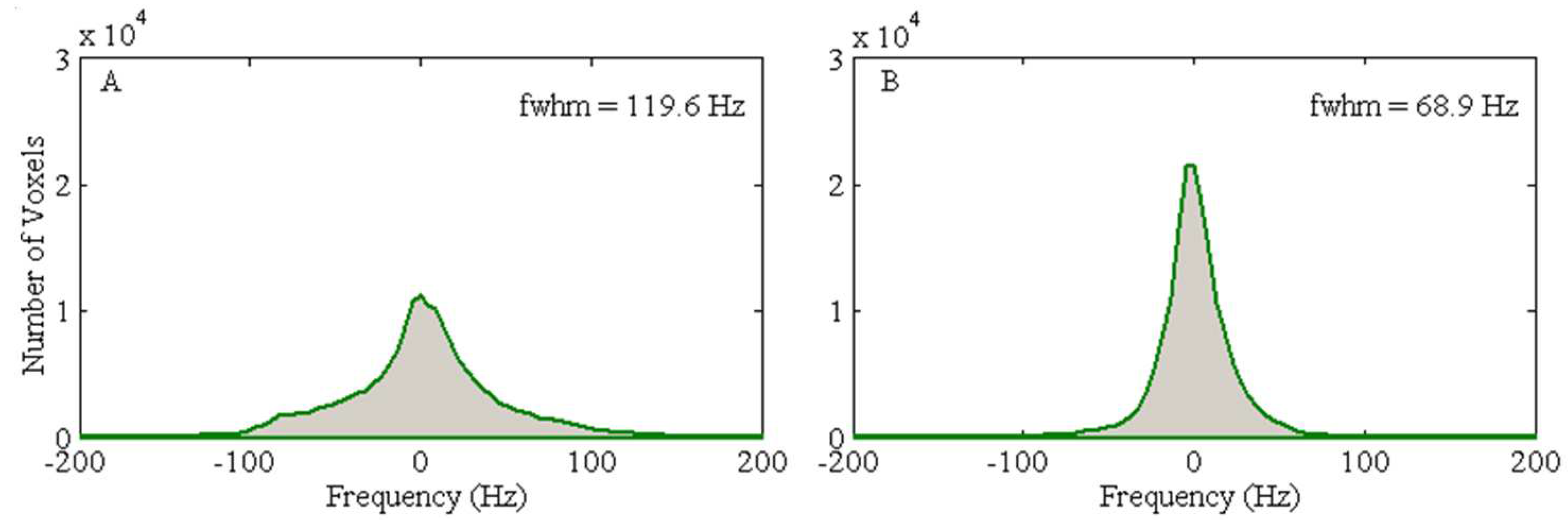
Figure 9.
The generation of the localized dipole passive shim field within the phantom. Axial, coronal, and sagittal slices of the magnetic field distribution within the phantom in the presence of local dipole passive shim system.
Figure 9.
The generation of the localized dipole passive shim field within the phantom. Axial, coronal, and sagittal slices of the magnetic field distribution within the phantom in the presence of local dipole passive shim system.
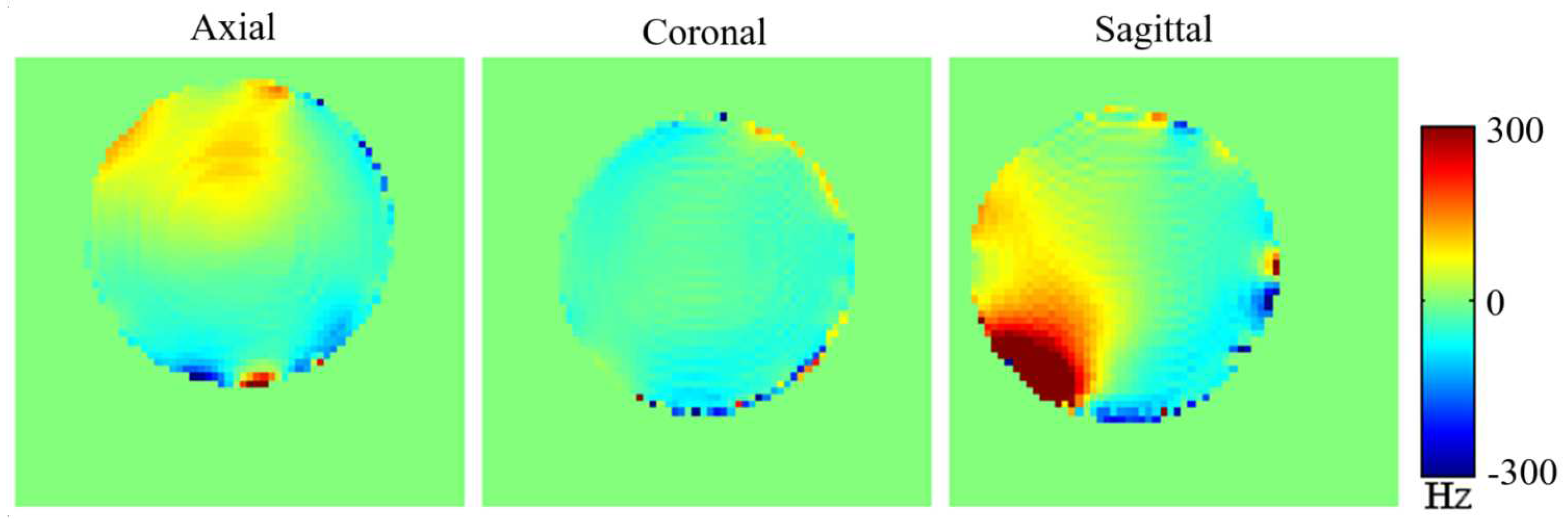
Figure 10.
The field maps by active shimming only and by the combination of both active and local dipole passive shimming of the 3rd subject’s orbitofrontal cortex region at 4T were compared. The field with (A) active shimming only, and (B) both active and local dipole passive shimming are presented. The field inhomogeneity over the OFC region remained after active shimming alone but was reduced after the introduction of a local dipole passive shimming.
Disclaimer/Publisher’s Note: The statements, opinions and data contained in all publications are solely those of the individual author(s) and contributor(s) and not of MDPI and/or the editor(s). MDPI and/or the editor(s) disclaim responsibility for any injury to people or property resulting from any ideas, methods, instructions or products referred to in the content. |
© 2024 by the authors. Licensee MDPI, Basel, Switzerland. This article is an open access article distributed under the terms and conditions of the Creative Commons Attribution (CC BY) license (http://creativecommons.org/licenses/by/4.0/).
Copyright: This open access article is published under a Creative Commons CC BY 4.0 license, which permit the free download, distribution, and reuse, provided that the author and preprint are cited in any reuse.


