Submitted:
26 January 2024
Posted:
26 January 2024
You are already at the latest version
Abstract
We construct hypergraphs to analyze functional brain connectivity, leveraging event-related coherence in magnetoencephalography (MEG) data during the visual perception of a flickering image. Principal network characteristics are computed for delta, theta, alpha, beta, and gamma frequency ranges. Employing a coherence measure, a statistical estimate of correlation between signal pairs across frequencies, we generate edge time series, depicting how an edge evolves over time. This forms the basis for constructing an edge-to-edge functional connectivity network. Emphasizing hyperedges as connected components in an absolute-valued functional connectivity network, we focus on exploring these hyperedges in the context of individual variability. Our coherence-based hypergraph construction specifically addresses functional connectivity among four brain lobes: frontal, parietal, temporal, and occipital. This approach enables a nuanced exploration of individual differences within diverse frequency bands, providing insights into the dynamical nature of brain connectivity during visual perception tasks. The results furnish compelling evidence supporting the hypothesis of cortico-cortical interactions occurring across varying scales. The derived hypergraph illustrates robust activation patterns in specific brain regions, indicative of their engagement across diverse cognitive contexts and different frequency bands. Our findings suggest potential integration or multifunctionality within the examined lobes, contributing valuable perspectives to our understanding of brain dynamics during visual perception.
Keywords:
brain
; magnetoencephalography (MEG)
; network
; hypergraph
; coherence
1. Introduction
Understanding the intricacies of brain connectivity in response to diverse stimuli is crucial for unraveling the mechanisms underlying information processing and decision-making within the brain. This study delves into three essential forms of brain connectivity: structural, functional, and efficient [1,2,3,4]. Structural connectivity entails the identification of anatomical neural networks, revealing potential pathways for neural communication [5,6]. On the other hand, functional connectivity explores active brain regions exhibiting correlated frequency, phase, and/or amplitude [7]. Finally, effective connectivity utilizes information from functional connectivity to discern the dynamic flow of information within the brain [8,9].
Measurement of effective and functional connectivity can be conducted in both the frequency domain, employing methods such as coherence [10], and in the time domain, utilizing approaches like Granger causality [4] or artificial neural network-based functional connectivity [11]. When a sufficiently large population of neurons synchronizes, their electrical and magnetic activities become detectable outside the skull through techniques like electroencephalography (EEG) and magnetoencephalography (MEG) [12]. EEG measures return or bulk currents outside the neuron (secondary currents), while MEG captures ionic currents inside the neuron (primary currents). Notably, MEG holds a distinct advantage over EEG due to its superior spatial resolution, rendering it an exceptional tool for investigating and characterizing interactions between distinct brain regions [13].
To study functional connectivity, some researchers use approaches borrowed from graph theory [14]. Using connections between the biorhythms of the brain in its various parts, a model of a complex network is recreated, in which parts of the brain are considered as nodes, and the connection forces between them are considered as links [15,16]. Using this approach makes it possible to identify not only individual cognitive differences between subjects [17], but also helps to diagnose some diseases at an early stage [18,19,20] and also monitor the aging process [21,22,23,24]. One of the important measures to quantify neuronal synchrony is event-related coherence [10,25,26]. It examines the frequency-domain relationship between two signals, indicating the degree to which their spectral components are synchronized. Essentially, it is an assessment of the constancy of the relative amplitude and phase between two signals within a given frequency range. There is a linear mathematical method that creates a symmetrical matrix, devoid of any directional information. Identical signals produce a coherence value of 1, while the coherence value approaches 0 as the difference between the signals in question increases. Since then, coherence has been used in many brain connectivity studies in patients and healthy individuals, including but not limited to studies of working memory [27], brain lesions [28], hemiparesis [29], resting state networks [30], schizophrenia [31,32], favorable responses to panic medications [33], and motor imagery [34]. Due to the individuality of human brains, different patterns of coherent neuronal activity were found in different subjects. For example, the presentation of flickering visual stimuli evokes in subjects coherent responses of the visual cortex to the flicker frequency and its harmonics with different sizes of coherent neural networks [35,36].
To study functional connectivity in this work we use hypergraph analysis, a method from dynamic graph theory [37]. We examine individual differences in functional connectivity networks in MEG data obtained while subjects view a flickering image. The method is based on a generalization of standard graph theory methods. Specifically, by defining a standard functional network of connectivity between nodes over successive periods, we create a set of edge time series, that is, a vector of how an edge changes over time. An edge-to-edge functional connectivity network is constructed by processing these edge time series similarly to the node time series in the first stage and computing the connections between each pair of edges. Here, we focus on “hyperedges,” which are the connected components of an end-to-end absolute-valued functional connectivity network.
To create the networks, we use the coherence measure defined as a statistical estimate of the correlation between pairs of signals as a function of frequency. The brain generates electromagnetic activity in a wide frequency range, from slow waves of 0.5 Hz to very fast waves of 500 Hz or more [38]. These rhythms are classified according to their frequency and are assigned Greek letters. We consider the five main frequency bands, each with distinctive characteristics. Delta waves (0–4 Hz) are the slower rhythms, have a greater amplitude, and predominate in deep sleep states. Theta rhythms (4–7 Hz) are present both during sleep and in waking states. Alpha rhythms (8–13 Hz) are characteristic of the waking state, predominantly in the occipital area. Beta waves (15–30 Hz) are higher frequency rhythms. Gamma rhythms (30–90 Hz) are the fastest, indicative of an active and alert cerebral cortex. The coherence measures correlations within discrete frequency bands for selected epoch lengths and is mathematically independent of signal amplitude [39]. In this work, we construct a hypergraph of functional connectivity based on coherence between four brain lobes: frontal, parietal, temporal, and occipital.
2. Materials and Methods
In this study, we analyze the MEG data of 15 healthy subjects (age: 17 to 64 years; 10 males) obtained in the experiment based on a flickering image paradigm [40] at the Center for Biomedical Technology of the Universidad Politécnica de Madrid, Spain. The MEG data have been downloaded from https://zenodo.org/record/44 08648#.X-72UdYo-Cc.
2.1. Stimulus
The employed stimulus consisted of presenting an image of a gray square whose pixels’ intensity was varied between different shades of gray. Brightness modulation of pixels was performed using a harmonic signal with a frequency of Hz and a maximum amplitude of 50% of the RGB color model, i.e., between black (0) and grey (127). This frequency was chosen due to its ability to generate a prominent spectral response in the visual cortex [35].
2.2. Experimental Protocol
The first stage of the experiment consisted of presenting a static square with a red dot in the center, to which the participants were instructed to maintain their gaze for 120 seconds. After a brief break, the modulated stimulus was presented, with the square changing the grey scale. The latter was presented 2 to 5 times at intervals of 120 s, with a 30-s break between each presentation.
2.3. Signal Analysis in Brainstorm
The signal analysis was performed using the Brainstorm software. Brainstorm is a collaborative, open-source application based on MATLAB dedicated to processing and analyzing brain recordings obtained by different brain imaging techniques [41]. The tools included, along with the interface, facilitated the creation of the scripts used in this article.
2.4. Head Model Adjustment
The default Brainstorm head model was adjusted to the head points recorded using a Polhemus Fastrak system, with 2% deformation and automatic refinement of head points.
2.5. Signal Processing
Signal analysis involved reading MEG data, and applying a Notch filter to eliminate 50-Hz power line frequencies and their harmonics. Artifacts from electrooculogram (EOG) and electrocardiogram (ECG) signals were automatically identified and manually reviewed to ensure the inclusion of any potentially omitted artifacts. Signal-space projection (SSP) methods were applied to correct artifacts by order.
2.6. Event Segmentation
The signals were segmented into 120-s epochs for two experimental steps: step B (background, no modulation) and step F (flickering image). The signal recorded during the B section was used as a reference signal. These epochs were further divided into 3-s trials.
2.7. Source Reconstruction
Reconstruction of electrical activity in the brain from MEG measurements was done by creating a forward model and a lead field matrix. Brainstorm’s overlapped spheres method was used, maintaining the recommended 15000 cortical sources. The inverse solution was calculated using standardized low-resolution electromagnetic tomography (sLORETA).
2.8. Signal Coherence
Network construction was based on coherence calculated between signals, a mathematical measure quantifying synchronization patterns between spatially separated sensors or between brain areas [42]. The strength of network interactions was estimated according to coherence between 8 brain areas (frontal left FL, frontal right FR, occipital left OL, occipital right OR, parietal left PL, parietal right PR, temporal left TL, temporal right TR). The 15000 brain sources were grouped into these 8 lobes using Brainstorm’s segmentation model, PALS-12 Lobes with 10 structures, excluding the insula, resulting in 8 structures or vertices.
The stored vertices were used to average signals within each lobe, reducing complexity to 8 signals. The square magnitude coherence was calculated between the time series of each lobe with the rest, for both F and B trials. This resulted in an coherence matrix with 1s on the main diagonal for each of the five frequency bands (delta, theta, alpha, beta, gamma), as illustrated in Fig. 1. Subsequently, the absolute difference between the coherence values of F and B was obtained and normalized to the B activity giving Event-Related Coherence (ERC) as
2.9. Visualization with BrainNet
The output consisted of a tensor with dimensions . The average matrix of all subjects was calculated for each frequency band, and these matrices were saved in ".edge" text files for visualization with BrainNet Viewer. The latter is a tool that facilitates the visualization of structural and functional connectivity patterns in brain networks [43]. The surface template used was "BrainMesh_ICBM152_smoothed.nv", included in the "BrainNetViewer_20191031" folder when downloaded.
A "Node.node" text file was created with the format defined by BrainNet Viewer to set the position of nodes in the brain figure. The ".edge" files for each frequency band obtained earlier were used to display interactions.
2.10. Fourier Analysis
Fast Fourier Transform (FFT) was used to show the dominant frequency of time series. Following [35] brain study with the same stimulus, frequency tags were identified at the blink frequency (6.67 Hz) and its harmonics. It was noted that frequency tags were more pronounced in the second harmonic (13.33 Hz) than in the first.
2.11. Graph Construction
Coherence matrices showed coefficients between 0.1 and 2. A threshold was set for graph construction, varying its value between 0.1 and 1.25. An analysis was conducted to assess how graph characteristics change when including interactions above .
Various centrality measures were calculated, such as degree centrality (number of edges [44]), betweenness centrality (fraction of shortest paths passing through a node [45]), and eigenvector centrality (importance of a node considering the importance of its neighbors [44]). Connected components of the graphs were explored [45]. The shortest path distances between all node pairs were calculated, and cycles in the graph were identified, and defined as connected graphs in which each vertex has degree 2 [46].
A threshold value of 0.45 was decided upon, as lower values show coherence interactions that include noise, and values higher than this completely lose one of our frequency bands.
With the determined threshold, graphs explicitly showing the mentioned measures were obtained using MATLAB functions.
2.12. Hypergraph Construction
To contextualize the analysis of hypergraphs, we define the elements of graph theory used to construct hypergraphs formed by nodes and edges, where nodes denote brain regions, or groups of voxels, and edges denote correlations in activity between pairs of nodes over time. Significant correlation in activity between pairs of edges over time is denoted as links. In this context, we define hyperedge as a group of links connecting two or more edges with significantly correlated temporal profiles. Finally, a set of hyperedges forms a hypergraph.
The algorithm of [47] was used for part of the hypergraph visualization. The incidence matrix was given as input. The obtained representations included the hypergraph, the incidence matrix in linear form, star expansion, and the adjacency tensor.
Hypergraph characteristics were obtained along with some matrix representations of the same.
2.12.1. Degrees of vertices and hyperedges
The degrees of the vertices of the hypergraph were calculated. It was determined as which is the number of vertices incident on . The degree of an edge is the number of vertices it contains, that is, .
2.12.2. 2-Section of the hypergraph
The 2-section of the hypergraph was obtained, which vertices are the vertices of H and where two distinct vertices form an edge if and only if they are in the same hyperedge of H [48].
2.12.3. Adjacency and node stars
Adjacency between vertices is found when at least one hyperedge contains the two vertices [14]. From here you can observe the stars of the nodes. Which are defined as the collection of hyperedges incident on a node i, is called the star of i.
2.12.4. Incidence between hyperedges
The incidence between the hyperedges was also considered. It is defined that two hyperedges and are said to be incident if , i.e., if they have at least one node in common [14]. The matrix of incidence can be obtained directly from the adjacency matrix of the bipartite diagram .
2.12.5. Relationship frequency matrix
The hypergraph relationship frequency matrix is another useful matrix that is defined as
That is the result of
2.12.6. Transverse and independent vertex sets
A set of vertices, T, is transversal if for each edge of our hypergraph, there is a vertex in T that is incident on that edge. The hypergraph is characterized with a transversal number , the size of the transversal minima of the hypergraph [48][46]. The independent set, S, is a set of vertices that do not contain an edge as a subset (in other words, there does not exist an edge incident only to vertices in S). This set is obtained from a hypergraph where the set T is a transversal, then is an independent set [48][46].
2.12.7. Coincidence between edges and coverage numbers
The coincidence between the edges of the hypergraph was examined. A set of edges, M, is said to be matching if the edges in M are pairwise disjoint [48][46]. Additionally, the coverage number was determined. A set, C, of edges is a covering if for every vertex in our hypergraph, there is an edge in C that is incident to that vertex [48]. The clique coverage number was calculated, which indicates the size of the smallest set of cliques that exhausts the vertices of the graph [46].
2.12.8. Line graph
The line graph of the hypergraph is also presented. Given our hypergraph , the line graph, , is the one whose vertex set is E, where a pair of vertices and in are adjacent when their corresponding edges in the hypergraph share an incident vertex (when )[46].
The nature of the intersection of the hypergraph families was characterized. Intersecting families are said to exist if all pairs of edges have a non-empty intersection, or equivalently if is a complete graph. With this analysis, we can know if the hypergraph complies with the Helly property, i.e., if is a star for every intersecting subfamily of H.
3. Results and Discussion
3.1. Coherence matrices
Coherence matrices were obtained for each frequency band, presented in the BrainNet Viewer template (Figure 1). One can observe strong coherence between temporal right and left lobes for delta waves (Figure 1a), frontal right and parietal and occipital right lobes for theta waves (Figure 1b), frontal left/right and parietal right/left lobes for alpha waves (Figure 1c), frontal right and parietal left lobes for beta waves (Figure 1d), and parietal and occipital lobes for gamma waves (Figure 1e). These findings are most effectively illustrated in the left panel of the sections of Figure 1, specifically in the brain representation. The peak coherence values are prominently depicted in the color bar, appearing as a distinct shade of dark red. In the matrix, the color corresponding to the highest coherence value is represented as yellow.
The presence of delta band oscillatory activity, commonly associated with slow-wave sleep [49], raises the question of whether delta band oscillations observed during both slow-wave sleep and wakeful states signify the same underlying phenomenon. Our study reveals a noteworthy coherence in delta activity. Research has connected delta band oscillations in specific cortical areas with attention [50]. Thus, our results suggest that coherence may find support in the context of these findings.
Additionally, it is noteworthy that our representation emphasizes the heightened connectivity of low-frequency components compared to high frequencies, aligning with previous observations by Salvador et al. [51]. This depiction offers a clearer insight into the variations in connectivity between lobes within each frequency band.
3.2. Power spectra
Figure 2 illustrates the modulated activity of each brain lobe, i.e. the absolute value of the signal representation in the frequency domain.
The modulation frequency Hz (M) is distinctly discernible in the power spectrum of the temporal right lobe. Simultaneously, its second harmonic Hz (H) is evident in the power spectra of both occipital and parietal lobes, spanning both the right and left hemispheres. This observation aligns cohesively with findings reported by Chholak et al. [40].
3.3. Network characteristics
Coherence allowed the comparison of the maximum coefficients achieved in each frequency band, ranging from 0 to 2.468. A general decrease in the coherence coefficient between nodes was observed with increasing frequency. As previously highlighted, our graph analyses encompass degree centrality, betweenness centrality, eigenvalue centrality, connected components, shortest-path distances, number of cycles, and node degrees.
The dynamics of the graph measurements are illustrated in Figure 3, Figure 4, Figure 5, Figure 6 and Figure 7, where we plot the coefficients with respect to coherence threshold for different brain waves (delta Figure 3; theta Figure 4; alpha Figure 5; beta Figure 6; gamma Figure 7). The lobes are represented with different colors. The graphical representations of shortest path distances and numbers of cycles depict averages in the case of distances and totals in the case of cycles.
One can see that for each frequency range, there is a coherence threshold value of at which centrality measures, shortest-path distances, and degree of nodes undergo significant changes. This threshold value depends on the wave frequency. Specifically, for delta and theta waves , for alpha waves , for beta waves , and for gamma waves . This means that decreases as the wave frequency increases, i.e., the brain network of functional connectivity is more stable in a low-frequency range.
In the degree centrality panel, it is notable that in the delta frequencies (Figure 3a), when values are below 0.5, certain lobes exhibit a degree centrality of 8. However, as values increase, a decrement in degree centrality is observed. Interestingly, the left parietal lobe becomes the first node to be entirely disconnected, a disconnection that manifests earlier at higher frequencies (Figure 5a–Figure 7a), where lower coefficients are evident even at low values. Contrastingly, betweenness centrality experiences a more rapid decay to 0 at high frequencies (Figure 5b–Figure 7b) compared to lower frequencies (Figure 3b–Figure 4b). In the case of eigenvalue centrality, the coefficient stabilizes around an approximate value of 1.3, with a longer duration needed to reach this value at lower frequencies (Figure 3c–Figure 4c) than at higher ones (Figure 5c–Figure 7c). Moreover, it is crucial to note that node behaviors exhibit frequency-dependent variations.
Examining connected components provides insights into the formation of bins. At delta frequencies (Figure 3d), nodes remain connected across most values until approximately 1.2, when a new bin emerges due to the disconnection of the left parietal lobe.
Figure 8 illustrates the results of the analysis of degree centrality in the brain network of the 8 lobes for the different frequency ranges. The node sizes indicate their importance as a function of edge weights. One can see that the connectivity is stronger in a low-frequency range, i.e., for delta and theta waves, and very weak for beta and gamma waves (Figure 8d and Figure 8e, respectively). Centrality, as extensively documented in the electrophysiological literature, has consistently underscored the non-uniform distribution of coherence across frequencies [52]. It has been well-established that different systems of brain regions may exhibit varying levels of coherence at distinct frequencies [51]. The centrality patterns also demonstrate frequency-specific nuances. Specifically, at lower frequencies, centrality predominantly manifests in the frontal lobes, with noteworthy lateralization observed in theta waves (Figure 8b). In the case of beta waves (Figure 8d), centrality becomes less distinct, and coefficients show a tendency to converge among nodes. Notably, gamma waves (Figure 8e) reveal a shift in centrality, now prominently observed in the occipital lobe.
Figure 9 displays another representation of the node degrees for the lobes. One can see that the nodes exhibit more uniform coherence-related connections considering low-frequency bands (Figure 9a-b). Note that in the higher-frequency range (Figure 9c-e), the connections are weaker, depending on the threshold chosen. However, the connections in the delta band (Figure 9a) are smaller compared to the theta network (Figure 9b), which is completely connected. Notably, a more evident alteration is evident in the alpha waves (Figure 9c), where only the right frontal lobe maintains a degree of 7, while the other lobes experience a reduction in connections. Within the beta graph (Figure 9d), both occipital lobes, along with the left frontal and left temporal lobes, cease to participate entirely, while the rest show a grade of 1. Meanwhile, in the gamma waves (Figure 9e), engagement diminishes for the left frontal, right frontal, and right temporal lobes, with a noteworthy contribution reemerging from the occipital lobes. Particularly, the right occipital lobe demonstrates the highest degree, marked at 2, within this band.
Figure 10 represents the results of the analysis of the betweenness centrality coefficient, which quantifies the importance of a node in terms of the geodesics passing through it. Again, the connections at higher frequencies are weaker (Figure 10c-d) than at lower frequencies (Figure 10a-b). One can also see that the nodes with higher betweenness centrality vary in different frequency bands. In both the beta and gamma graphs (Figure 10c-d), the nodes exhibit a uniform and reduced size. Interestingly, at the delta frequency, the nodes with the highest degree centrality in the graph (Figure 8a; specifically, the left frontal, right frontal, left temporal, and right temporal lobes) undergo a reduction in size in the betweenness centrality graph (Figure 10a). Contrarily, in the theta graph (Figure 10b), a marked enlargement is observed in the left frontal lobe compared to the other lobes, presenting a notable contrast to the sizes depicted in the degree centrality graph (Figure 8b), where it initially appeared to be the smallest.
Eigenvector centrality which measures the importance of a node in terms of the importance of its neighbors, is presented in Figure 11. Node sizes indicate their importance, which shows the same patterns as those seen in Figure 8. Whereas, for beta waves, the nodes show the same size.
Figure 12 depicts the connected graph components, i.e., the subset of network nodes such that there is a path from each node in the subset to any other node in the same subset [45]. The representation of connected graph components can provide valuable insights into the collaborative dynamics of distinct brain regions, particularly within different frequency ranges. By examining the functional connectivity patterns captured within these components, we gain a nuanced understanding of how various regions can coordinate their activities across the spectrum of brain oscillations.
Distances between nodes are represented as matrices (,,,,), showing the shortest path distances. When the nodes are not connected, the distance is infinite. The largest value is 2 node distance only seen in the alpha range.
Figure 13 presents cycles formed in the networks for three frequency bands: delta, theta, and alpha. A cycle is a connected graph in which each vertex has degree 2 [46]. The total number of cycles found for that graph is also shown. The theta graph (Figure 13b) is characterized by complete connectivity, thereby revealing the total number of cycles present within the network. In contrast, both the alpha and delta graphs (Figure 13c-a, respectively) exhibit fewer connections. This aligns with the broader concept in the literature suggesting that slower rhythmic patterns tend to encompass a more global network configuration compared to their faster counterparts [53,54].
3.4. Hypergraphs
Figure 14 represents the hypergraph constructed on the base of a chosen threshold in different forms with colors corresponding to different frequency bands. In particular, the hypergraph is shown as a network in Figure 14a, a star expansion in Figure 14b with connections for each node, and in a matrix form in Figure 14c. While all 8 lobes are coupled in the high-frequency ranges of the delta, theta, and alpha waves, only 4 lobes (FR, TR, PL, and PR) are coupled in the beta waves, and 5 lobes (TL, PL, PR, OL, and OR) in gamma waves.
The analysis was carried out following the basic properties of hypergraphs. The degrees of the vertices and hyperedges are given in Table 1, where is the number of vertices incident on , and the degree of an edge is the number of vertices it contains.

Table 1.
Vertices and hyperedges degrees.
| Vertice | |E()| | Hyperedge | |e| |
|---|---|---|---|
| Frontal Left | 3 | Delta | 8 |
| Frontal Right | 4 | Theta | 8 |
| Occipital Left | 4 | Alpha | 8 |
| Occipital Right | 4 | Beta | 4 |
| Parietal Left | 5 | Gamma | 5 |
| Parietal Right | 5 | ||
| Temporal Left | 4 | ||
| Temporal Right | 4 |
The 2-section of the hypergraph is presented in Figure 15, where FL, FR, TL, TR, PL, PR, OL, OR constitutes the maximum clique in the 2-section, and it is also an edge in the hypergraph. Three of the hyperedges in the hypergraph are maximal cliques, and all nodes in the hypergraph are adjacent due to the definition of adjacency in hypergraphs. An all-to-all connectivity is shown by the 2-section of the hypergraph, i.e., that all nodes are interconnected. This is due to the presence of at least one lobe participating in both frequency bands. This underscores that certain brain regions are active across multiple contexts or tasks associated with different frequency bands. This observation implies the potential existence of some form of integration or multifunctionality within the lobes.
A star, as mentioned earlier, denotes a pattern where a central vertex, representing in this case, a cerebral lobe, is intricately connected to multiple peripheral vertices, symbolizing different brain frequency ranges. This graphical representation is valuable as it effectively portrays the intricate relationship between a specific cerebral lobe and its involvement across diverse frequency bands. The presence of stars within the graph signifies that the central cerebral lobe exhibits activation across various cognitive conditions or mental states, indicative of its multifunctional nature.
The stars of each lobe are the following:
- -
- Left Frontal Lobe (node 1): Delta, theta, alpha.
- -
- Right Frontal Lobe (node 2): Delta, theta, alpha, beta.
- -
- Left Occipital Lobe (node 3): Delta, theta, alpha, gamma.
- -
- Right Occipital Lobe (node 4): Delta, theta, alpha, gamma.
- -
- Left Parietal Lobe (node 5): Delta, theta, alpha, beta, gamma.
- -
- Right Parietal Lobe (node 6): Delta, theta, alpha, beta, gamma.
- -
- Left Temporal Lobe (node 7): Delta, theta, alpha, gamma.
- -
- Right Temporal Lobe (node 8): Delta, theta, alpha, beta.
Furthermore, the identification of parietal lobes emerges as noteworthy, given their coordination across all frequency bands. Correlations between frequencies have been observed in previous studies [55] and biophysical models have been proposed to explain interactions among different frequencies, such as theta and gamma in [56]. However, further research, such as the current study, is necessary to elucidate a potential coupling between the mechanisms generating these distinct frequencies.
The incidence matrix is obtained directly from the adjacency matrix of the bipartite diagram :
The frequency matrix of relations of H, , is
All hyperedges are included as a part of another hyperedge. Multiple hyperedges are only found in the delta, theta, and alpha regions containing the same nodes. The set of vertices LP, RP is a transversal since they are included in all edges. The transversal number is with the minimum transversals being LP and RP.
From the set of vertices, removing T yields an independent set LF, RF, LO, RO, LT, RT, as illustrated in Figure 16. The edges of the hypergraph are connected, sharing at least 1 vertex all of them, so there is no set of coincident edges. This satisfies the coincident/transverse relation, since .
The set of delta, theta, alpha, beta, and gamma waves is a cover since all edges are represented by at least one hyperedge.
Therefore, the coverage number of the hypergraph is
The clique cover number of the graph G is also
Figure 17 represents the line graph. The vertices are linked because they have a hyperedge in common. It is satisfied that . This means that the 2-section of a hypergraph is isomorphic to the line graph of the dual of the hypergraph. While the line graph offers a straightforward and overarching perspective on the interconnections among hyperedges, the 2-section delves into greater detail by incorporating both hyperedges and individual elements within a unified framework. However, it upholds the previously mentioned implications.
The evaluation of the intersecting families shows that they are non-empty, all hyperedges being incident, i.e.
The line graph is complete. All stars are intersecting families. Fulfilling this condition, H is a Helly hypergraph. This satisfies that if H is Helly and has no empty edges, then .
4. Conclusions
In this paper, we conducted a comprehensive hypergraph analysis of functional connectivity based on event-related coherence using MEG data obtained from visual perception experiments. By specifically examining individual differences within diverse frequency bands, we developed a coherence-based hypergraph to investigate functional connectivity among different brain lobes, namely frontal, parietal, temporal, and occipital. Our findings provide support for the hypothesis that cortico-cortical interactions may occur at various scales. The resulting hypergraph reveals robust activation patterns in specific brain regions across diverse cognitive contexts associated with different frequency bands, suggesting potential integration or multifunctionality within these lobes.
The identification of stars in our graphical analysis emphasizes the multifunctional nature inherent in the central lobes of the brain. These lobes exhibit close connections to peripheral vertices, representing distinct frequency ranges within the brain. This perspective effectively highlights the varied engagement of specific lobes in diverse cognitive or mental states. Moreover, the central role played by the parietal lobes in coordinating across all frequency ranges underscores the significance of information integration in various cognitive processes.
While prior studies have observed correlations between frequencies and proposed biophysical models to explicate interactions, our study emphasizes the need for additional research to unravel potential connections between mechanisms generating different frequencies. Furthermore, we contend that delving into hypergraph visualizations with a concentrated exploration of finer-grained neural ensembles or smaller regions of interest (ROIs) can unveil captivating dynamics worthy of scholarly investigation.
Author Contributions
N.P.S.: investigation, formal analysis; R.J.R.: resources, project administration, original draft preparation; A.N.P.: conceptualization, methodology, review and editing.
Conflicts of Interest
‘The authors declare no conflicts of interest. The funders had no role in the design of the study; in the collection, analyses, or interpretation of data; in the writing of the manuscript; or in the decision to publish the results’.
References
- Friston, K.J.; Frith, C.D.; Liddle, P.F.; Frackowiak, R.S. Functional connectivity: the principal-component analysis of large (PET) data sets. J. Cereb. Blood Flow Metab. 1993, 13, 5–14. [Google Scholar] [CrossRef]
- Greenblatt, R.E.; Pflieger, M.E.; Ossadtchi, A.E. Connectivity measures applied to human brain electrophysiological data. J. Neurosci. Methods 2012, 207, 1–16. [Google Scholar] [CrossRef]
- Greenblatt, R.E.; Pflieger, M.E.; Ossadtchi, A.E. Review of advanced techniques for the estimation of brain connectivity measured with EEG/MEG. Comput. Biol. Med. 2011, 41, 1110–1117. [Google Scholar]
- Hramov, A.E.; Frolov, N.S.; Maksimenko, V.A.; Kurkin, S.A.; Kazantsev, V.B.; Pisarchik, A.N. Functional networks of the brain: from connectivity restoration to dynamic integration. Phys. Uspekhi 2021, 64, 584–616. [Google Scholar] [CrossRef]
- Le Bihan, D.; Mangin, J.F.; Poupon, C. snd Clark, C.A.; Pappata, S.; Molko, N.; Chabriat, H. Diffusion tensor imaging: concepts and applications. J. Magn. Reson. Imaging JMRI 2001, 13, 534–546. [Google Scholar] [CrossRef]
- Wedeen, V.J.; Wang, R.P.; Schmahmann, J.D.; Benner, T.; Tseng, W.Y.I.; Dai, G.; Pandya, D.N.; Hagmann, P.; D’Arceuil, H.; de Crespigny, A.J. Diffusion spectrum magnetic resonance imaging (DSI) tractography of crossing fibers. NeuroImage 2008, 41, 1267–1277. [Google Scholar] [CrossRef]
- Towle, V.L.; Hunter, J.D.; Edgar, J.C.; Chkhenkeli, S.A.; Castelle, M.C.; Frim, D.M.; Kohrman, M.; Hecox, K. Frequency domain analysis of human subdural recordings. J. Clin. Neurophysiol. 2007, 24, 205–213. [Google Scholar] [CrossRef]
- Cabral, J.; Kringelbach, M.L.; Deco, G. Exploring the network dynamics underlying brain activity during rest. Prog. Neurobiol. 2014, 114, 102–131. [Google Scholar] [CrossRef]
- Horwitz, B. The elusive concept of brain connectivity. NeuroImage 2003, 19, 466–470. [Google Scholar] [CrossRef]
- Bowyer, S. Coherence a measure of the brain networks: past and present. Neuropsychiatr. Electrophysiol. 2016, 2, 1. [Google Scholar] [CrossRef]
- Frolov, N.; Maksimenko, V.; Lüttjohann, A.; Koronovskii, A.; Hramov, A. Feed-forward artificial neural network provides data-driven inference of functional connectivity. Chaos 2019, 29, 091101. [Google Scholar] [CrossRef]
- Hämäläinen, M.; Hari, R.; Ilmoniemi, R.J.; Knuutila, J.; Lounasmaa, O.V. Magnetoencephalography – theory, instrumentation, and applications to noninvasive studies of the working human brain. Rev. Mod. Phys. 1993, 65, 413. [Google Scholar] [CrossRef]
- Burgess, R.C. Magnetoencephalography for localizing and characterizing the epileptic focus. Handb. Clin. Neurol. 2019, 160, 203–214. [Google Scholar]
- Boccaletti, S.; De Lellis, P.; del Genio, C.; Alfaro-Bittner, K.; Criado, R.; Jalan, S.; Romance, M. The structure and dynamics of networks with higher order interactions. Phys. Rep. 2023, 1018, 1–64. [Google Scholar] [CrossRef]
- Bullmore, E.; Sporns, O. Complex brain networks: graph theoretical analysis of structural and functional systems. Nat. Rev, Neurosci. 2009, 10, 186–198. [Google Scholar] [CrossRef]
- Friston, K.J. Functional and effective connectivity: a review. Brain Connectivity 2011, 1, 13–36. [Google Scholar] [CrossRef]
- Tavor, I.; Jones, O.P.; Mars, R.; Smith, S.; Behrens, T.; Jbabdi, S. Task-free MRI predicts individual differences in brain activity during task performance. Science 2016, 352, 216–220. [Google Scholar] [CrossRef]
- Zhang D, R.M. Disease and the brain’s dark energy. Nat. Rev. Neurol. 2010, 6, 15–28. [Google Scholar] [CrossRef]
- Greicius, M. Resting-state functional connectivity in neuropsychiatric disorders. Curr. Opin. Neurol. 2008, 21, 424–430. [Google Scholar] [CrossRef]
- Dennis, E.L.; Thompson, P.M. Functional brain connectivity using fMRI in aging and Alzheimer’s disease. Neuropsychol. Rev. 2014, 24, 49–62. [Google Scholar] [CrossRef]
- Tomasi, D.; Volkow, N.D. Aging and functional brain networks. Mol. Psychiatry 2012, 17, 549–558. [Google Scholar] [CrossRef]
- Contreras, J.A.; Goñi, J.; Risacher, S.L.; Sporns, O.; Saykin, A.J. The structural and functional connectome and prediction of risk for cognitive impairment in older adults. Curr. Behav. Neurosci. Rep. 2015, 2, 234–245. [Google Scholar] [CrossRef]
- Sala-Llonch, R.; Bartrés-Faz, D.; Junqué, C. Reorganization of brain networks in aging: a review of functional connectivity studies. Front. Psychol. 2015, 6. [Google Scholar] [CrossRef]
- Davison, E.N.; Turner, B.O.; Schlesinger, K.J.; Miller, M.B.; Grafton, S.T.; Bassett, D.S.; Carlson, J.M. Individual differences in dynamic functional brain connectivity across the human lifespan. PLoS Comput. Biol. 2016, 12, e1005178. [Google Scholar] [CrossRef]
- Andrew, C.; Pfurtscheller, G. Event-related coherence as a tool for studying dynamic interaction of brain regions. Electroencephalogr. Clin. Neurophysiol. 1996, 98, 144–148. [Google Scholar] [CrossRef]
- Pisarchik, A.; Hramov, A. Coherence resonance in neural networks: Theory and experiments. Phys. Rep. 2023, 1000, 1–57. [Google Scholar] [CrossRef]
- Gross, J.; Schmitz, F.; Schnitzler, I.; Kessler, K.; Shapiro, K.; Hommel, B.; Schnitzler, A. Modulation of long-range neural synchrony reflects temporal limitations of visual attention in humans. Proc. Natl. Acad. Sci. USA 2004, 101, 13050–13055. [Google Scholar] [CrossRef]
- Guggisberg, A.G.; Honma, S.M.; Findlay, A.M.; Dalal, S.S.; Kirsch, H.E.; Berger, M.S.; Nagarajan, S.S. Mapping functional connectivity in patients with brain lesions. Ann. Neurol. 2008, 63, 193–203. [Google Scholar] [CrossRef]
- Belardinelli, P.; Ciancetta, L.; Staudt, M.; Pizzella, V.; Londei, A.; Birbaumer, N.; Romani, G.L.; Braun, C. Cerebro-muscular and cerebro-cerebral coherence in patients with pre- and perinatally acquired unilateral brain lesions. NeuroImage 2007, 37, 1301–1314. [Google Scholar] [CrossRef]
- de Pasquale, F.; Della Penna, S.; Snyder, A.Z.; Lewis, C.; Mantini, D.; Marzetti, L.; Belardinelli, P.; Ciancetta, L.; Pizzella, V.; Romani, G.L.; Corbetta, M. Temporal dynamics of spontaneous MEG activity in brain networks. Proc. Natl. Acad. Sci. USA 2010, 107, 6040–6045. [Google Scholar] [CrossRef]
- Kim, J.S.; Shin, K.S.; Jung, W.H.; Kim, S.N.; Kwon, J.S.; Chung, C.K. Power spectral aspects of the default mode network in schizophrenia: an MEG study. BMC Neurosci. 2014, 15, 104. [Google Scholar] [CrossRef]
- Bowyer, S.M.; Gjini, K.; Zhu, X.; Kim, L.; Moran, J.E.; Rizvi, S.U.; Gumenyuk, N.T.; Tepley, N.; Boutros, N.N. Potential biomarkers of schizophrenia from MEG resting-state functional connectivity networks: Preliminary data. J. Behav. Brain Sci. 2015, 5, 1. [Google Scholar] [CrossRef]
- Boutros, N.N.; Galloway, M.P.; Ghosh, S.; Gjini, K.; Bowyer, S.M. Abnormal coherence imaging in panic disorder: a magnetoencephalography investigation. Neuroreport 2013, 24, 487–491. [Google Scholar] [CrossRef]
- Chholak, P.; Niso, G.; Maksimenko, V.A.; Kurkin, S.A.; Frolov, N.S.; Pitsik, E.N.; Hramov, A.E.; Pisarchik, A.N. Visual and kinesthetic modes affect motor imagery classification in untrained subjects. Sci. Rep. 2019, 9, 1–12. [Google Scholar] [CrossRef]
- Pisarchik, A.N.; Chholak, P.; Hramov, A.E. Brain noise estimation from MEG response to flickering visual stimulation. Chaos Solitons Fractals X 2019, 1, 100005. [Google Scholar] [CrossRef]
- Chholak, P.; Maksimenko, V.A.; Hramov, A.E.; Pisarchik, A.N. Voluntary and involuntary attention in bistable visual perception: a MEG study. Front. Hum. Neurosci. 2020, 14, 555. [Google Scholar] [CrossRef]
- Dai, Q.; Gao, Y. Hypergraph Computation; Springer: Singapore, 2023. [Google Scholar]
- Bear, M.; Connors, B.; Paradiso, M.A. Neuroscience: exploring the brain, enhanced edition: exploring the brain; Jones & Bartlett Learning, 2020.
- French, C.C.; Beaumont, J.G. A critical review of EEG coherence studies of hemisphere function. Internat. J. Psychophysiol. 1984, 1, 241–254. [Google Scholar] [CrossRef]
- Chholak, P.; Kurkin, S.A.; Hramov, A.E.; Pisarchik, A.N. Event-related coherence in visual cortex and brain noise: an MEG study. Appl. Sci. 2021, 11, 375. [Google Scholar] [CrossRef]
- Tadel, F.; Baillet, S.; Mosher, J.C.; Pantazis, D.; Leahy, R.M. Brainstorm: A user-friendly application for MEG/EEG analysis. Comput. Intell. Neurosci. 2011, 2011, 1–13. [Google Scholar] [CrossRef]
- Bowyer, S.M. Coherence a measure of the brain networks: past and present. Neuropsychiatr. Electrophysiol. 2016, 2, 1–12. [Google Scholar] [CrossRef]
- Xia, M.; Wang, J.; He, Y. BrainNet Viewer: a network visualization tool for human brain connectomics. PloS One 2013, 8, e68910. [Google Scholar] [CrossRef]
- Golbeck, J. Analyzing the Social Web; Morgan Kaufmann: Boston, 2013. [Google Scholar]
- Zinoviev, D. Complex Network Analysis in Python: Recognize-Construct-Visualize-Analyze-Interpret; Pragmatic Bookshelf, 2018.
- Voloshin, V.I. Introduction to Graph and Hypergraph Theory; Nova Science Publishers, 2009.
- Pickard, J.; Chen, C.; Salman, R.; Stansbury, C.; Kim, S.; Surana, A.; Bloch, A.; Rajapakse, I. HAT: hypergraph analysis toolbox. PloS Comput. Biol. 2023, 19, e1011190. [Google Scholar] [CrossRef]
- Bretto, A. Hypergraph Theory: An Introduction; Mathematical Engineering, Springer: Cham, 2013. [Google Scholar]
- Hobson, J.A.; Pace-Schott, E.F. The cognitive neuroscience of sleep: neuronal systems, consciousness and learning. Nat. Rev. Neurosci. 2002, 3, 679–693. [Google Scholar] [CrossRef]
- Saleh, M.; Reimer, J.; Penn, R.; Ojakangas, C.L.; Hatsopoulos, N.G. Fast and slow oscillations in human primary motor cortex predict oncoming behaviorally relevant cues. Neuron 2010, 65, 461–471. [Google Scholar] [CrossRef]
- Salvador, R.; Suckling, J.; Schwarzbauer, C.; Bullmore, E. Undirected graphs of frequency-dependent functional connectivity in whole brain networks. Phil. Trans. Roy. Soc. B 2005, 360, 937–946. [Google Scholar] [CrossRef]
- Sun, F.T.; Miller, L.M.; D’esposito, M. Measuring interregional functional connectivity using coherence and partial coherence analyses of fMRI data. Neuroimage 2004, 21, 647–658. [Google Scholar] [CrossRef]
- Von Stein, A.; Sarnthein, J. Different frequencies for different scales of cortical integration: from local gamma to long range alpha/theta synchronization. Int. J. Psychophysiol. 2000, 38, 301–313. [Google Scholar] [CrossRef]
- Buzsaki, G.; Draguhn, A. Neuronal oscillations in cortical networks. Science 2004, 304, 1926–1929. [Google Scholar] [CrossRef]
- Furl, N.; Coppola, R.; Averbeck, B.B.; Weinberger, D.R. Cross-frequency power coupling between hierarchically organized face-selective areas. Cereb. Cortex 2014, 24, 2409–2420. [Google Scholar] [CrossRef]
- Pastoll, H.; Solanka, L.; van Rossum, M.C.; Nolan, M.F. Feedback inhibition enables theta-nested gamma oscillations and grid firing fields. Neuron 2013, 77, 141–154. [Google Scholar] [CrossRef]
Figure 1.
Coherence networks with their respective matrices for (a) delta, (b) theta, (c) alpha, (d) beta, and (e) gamma waves. In the matrices, the lobes in order are: Left frontal (1), right frontal (2), left occipital (3), right occipital (4), left parietal (5), right parietal (6), left occipital (7 ), right occipital (8).
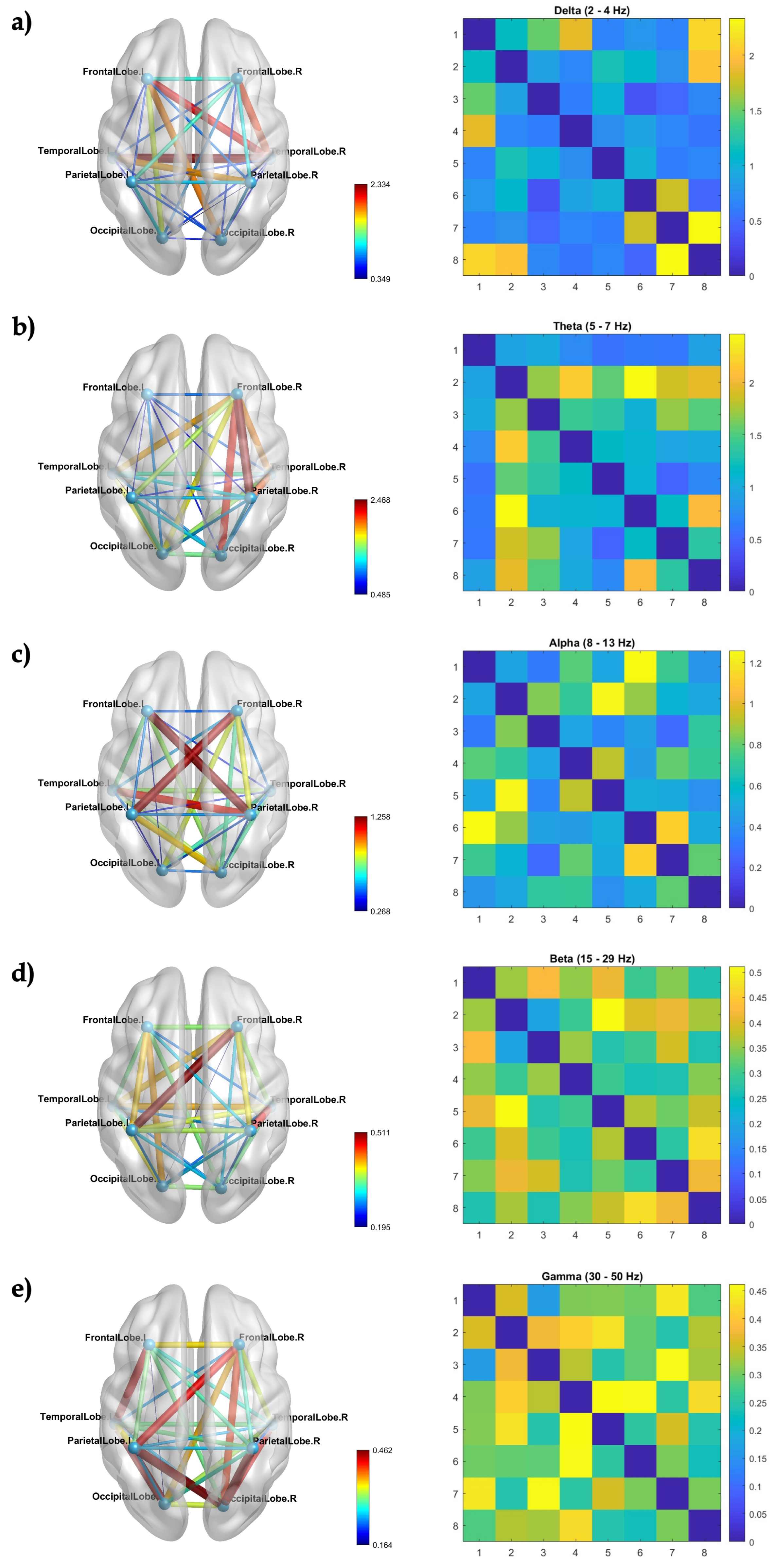
Figure 2.
FFT analysis of modulated activity in different brain lobes: (a) left frontal, (b) right frontal, (c) left occipital, (d) right occipital, (e) left parietal, (f) right parietal, (g) left temporal, and (h) right temporal. The dotted lines marked by letters M and H indicate the modulation frequency and its second harmonic , respectively.
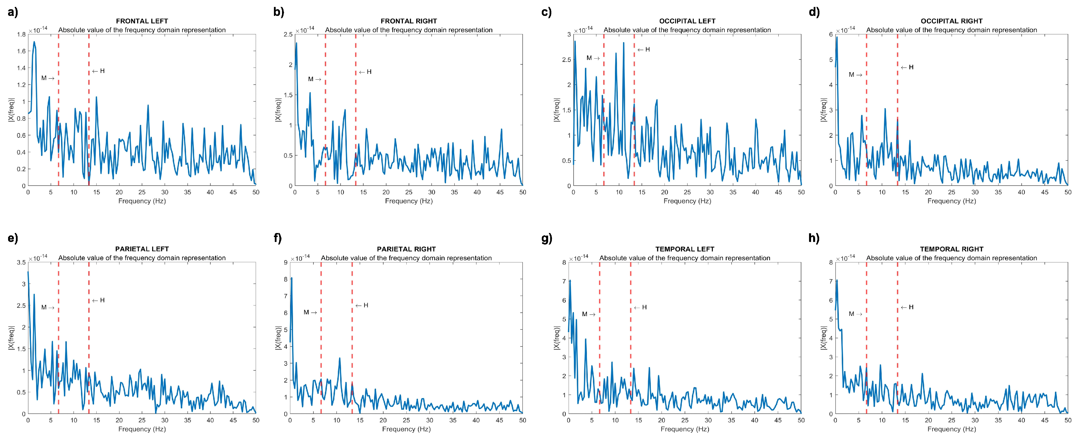
Figure 3.
Network characteristics versus coherence threshold value for delta waves: (a) degree centrality , (b) betweenness centrality , (d) connected components, (e) shortest-path distances d, (f) number of cycles , and (g) node degree .
Figure 3.
Network characteristics versus coherence threshold value for delta waves: (a) degree centrality , (b) betweenness centrality , (d) connected components, (e) shortest-path distances d, (f) number of cycles , and (g) node degree .
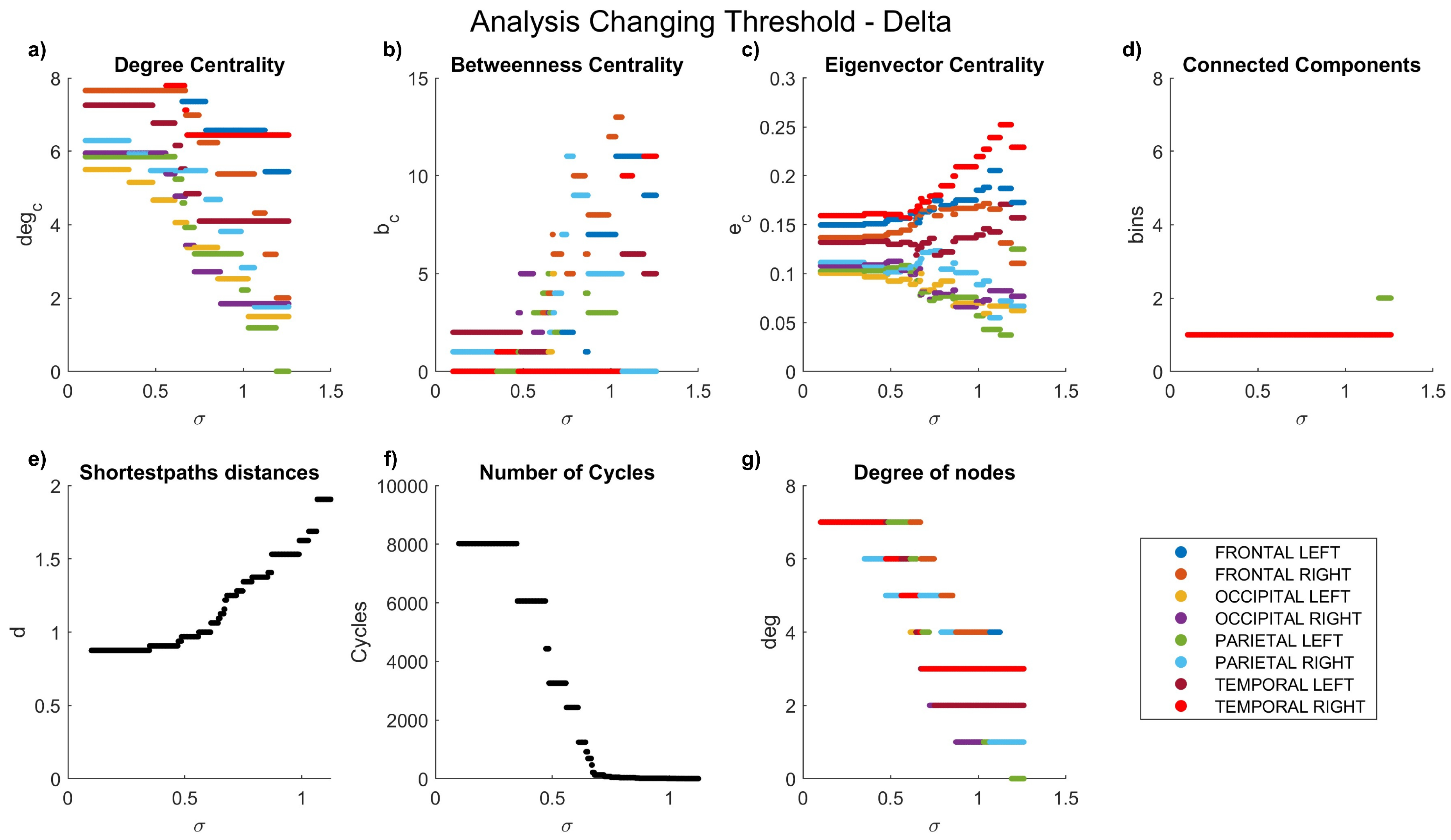
Figure 4.
Network characteristics versus coherence threshold value for theta waves: (a) degree centrality , (b) betweenness centrality , (d) connected components, (e) shortest-path distances d, (f) number of cycles , and (g) node degree .
Figure 4.
Network characteristics versus coherence threshold value for theta waves: (a) degree centrality , (b) betweenness centrality , (d) connected components, (e) shortest-path distances d, (f) number of cycles , and (g) node degree .
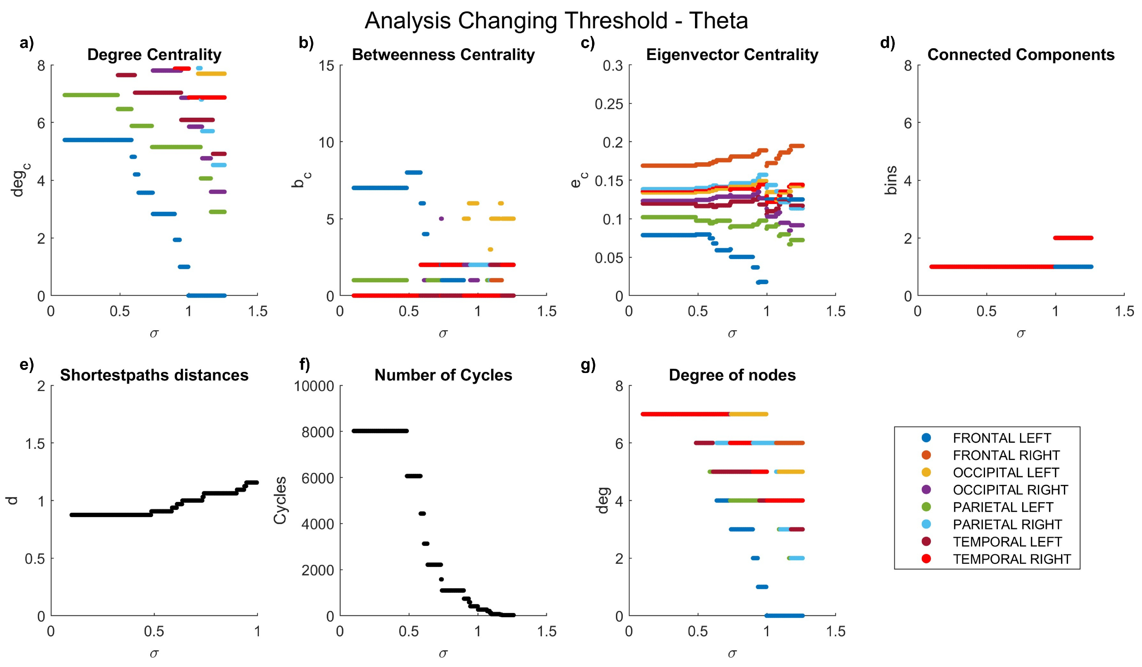
Figure 5.
Network characteristics versus coherence threshold value for alpha waves: (a) degree centrality , (b) betweenness centrality , (d) connected components, (e) shortest-path distances d, (f) number of cycles , and (g) node degree .
Figure 5.
Network characteristics versus coherence threshold value for alpha waves: (a) degree centrality , (b) betweenness centrality , (d) connected components, (e) shortest-path distances d, (f) number of cycles , and (g) node degree .
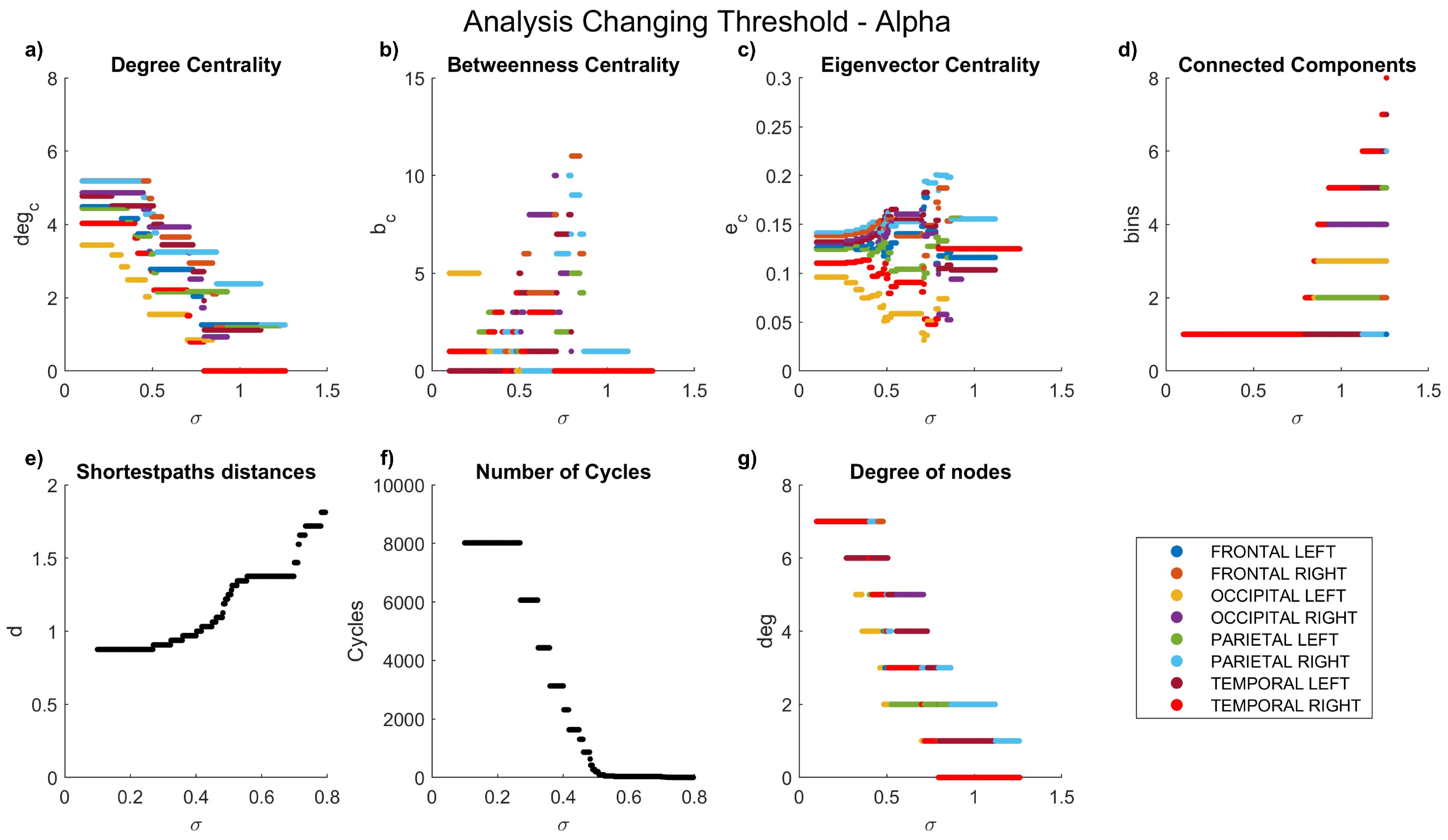
Figure 6.
Network characteristics versus coherence threshold value for beta waves: (a) degree centrality , (b) betweenness centrality , (d) connected components, (e) shortest-path distances d, (f) number of cycles , and (g) node degree .
Figure 6.
Network characteristics versus coherence threshold value for beta waves: (a) degree centrality , (b) betweenness centrality , (d) connected components, (e) shortest-path distances d, (f) number of cycles , and (g) node degree .
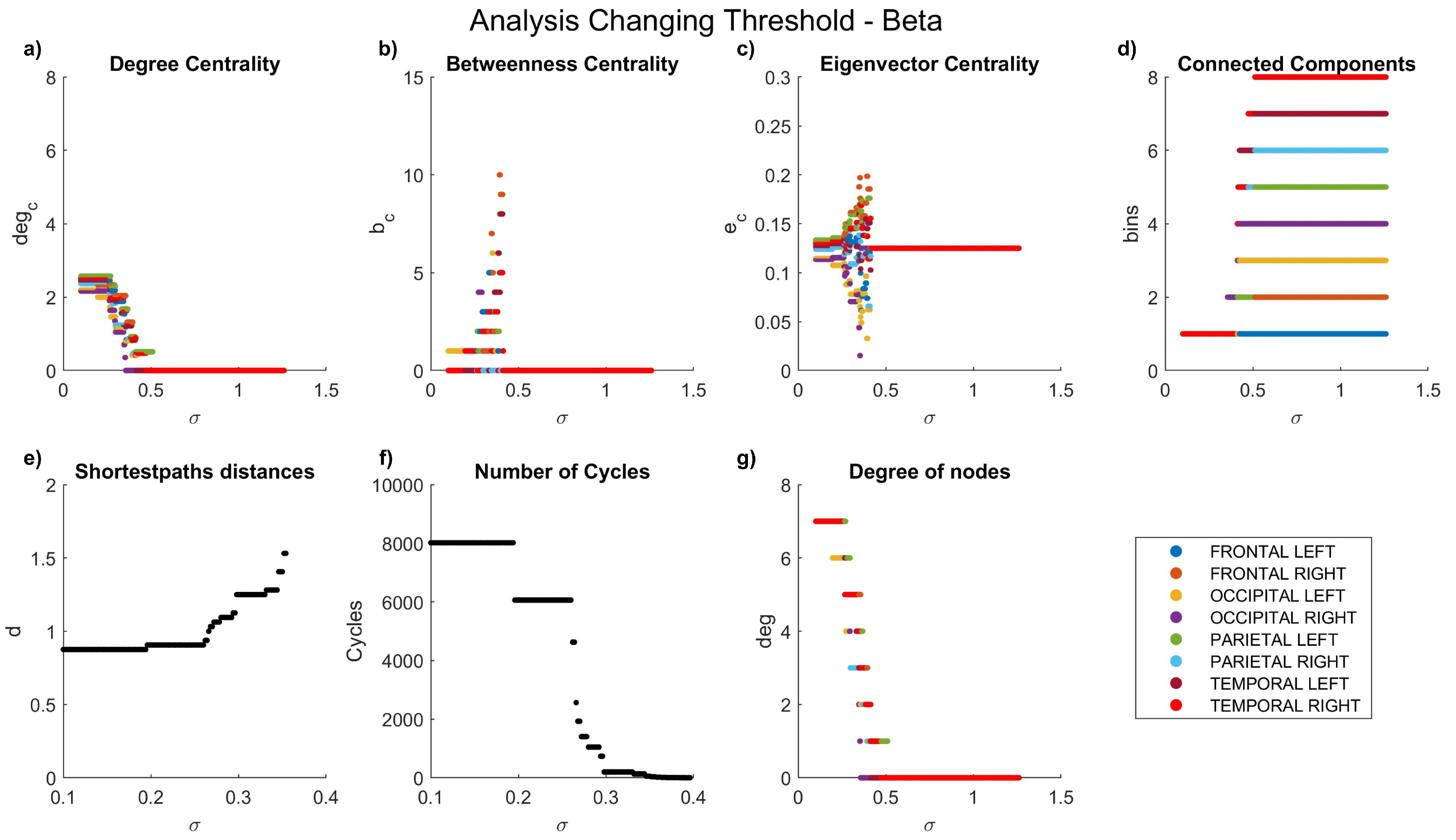
Figure 7.
Network characteristics versus coherence threshold value for gamma waves: (a) degree centrality , (b) betweenness centrality , (d) connected components, (e) shortest-path distances d, (f) number of cycles , and (g) node degree .
Figure 7.
Network characteristics versus coherence threshold value for gamma waves: (a) degree centrality , (b) betweenness centrality , (d) connected components, (e) shortest-path distances d, (f) number of cycles , and (g) node degree .
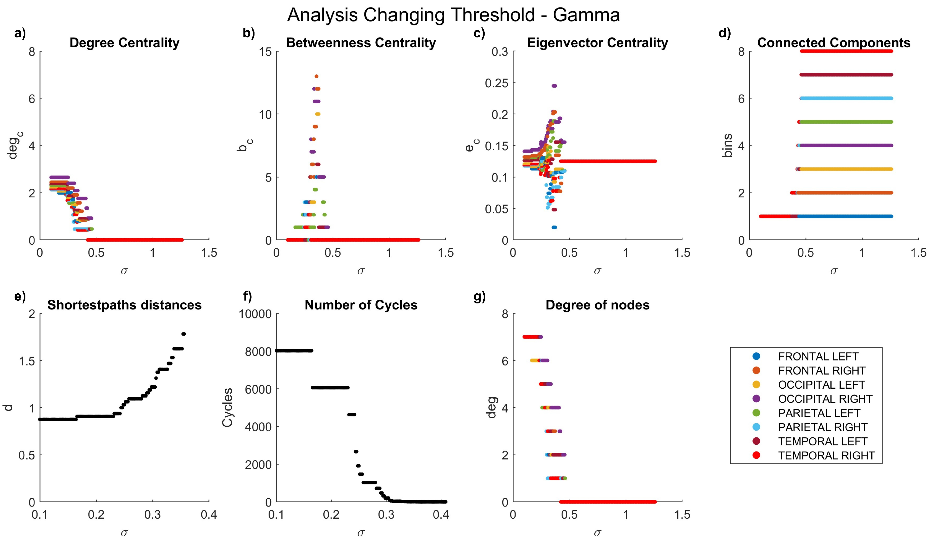
Figure 8.
Degree centrality for (a) delta, (b) theta, (c) alpha, (d) beta, and (e) gamma waves at .
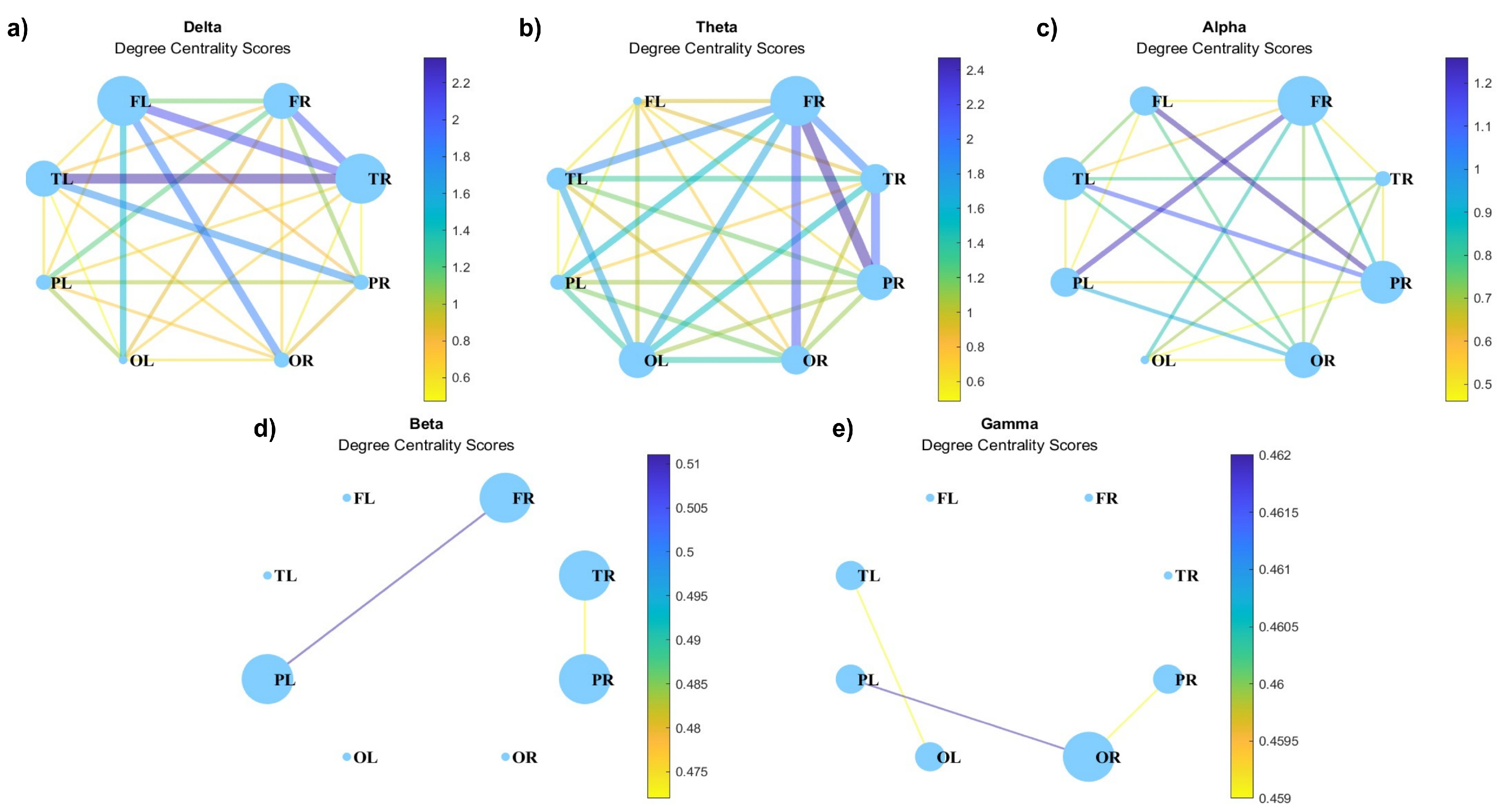
Figure 9.
Node degrees for (a) delta, (b) theta, (c) alpha, (d) beta, and (e) gamma waves. FL – Left frontal, FR – Right frontal, OL – Left occipital, OR – Right occipital, PL – Left parietal, PR – Right parietal, TL – Left temporal, TR – Right temporal.
Figure 9.
Node degrees for (a) delta, (b) theta, (c) alpha, (d) beta, and (e) gamma waves. FL – Left frontal, FR – Right frontal, OL – Left occipital, OR – Right occipital, PL – Left parietal, PR – Right parietal, TL – Left temporal, TR – Right temporal.
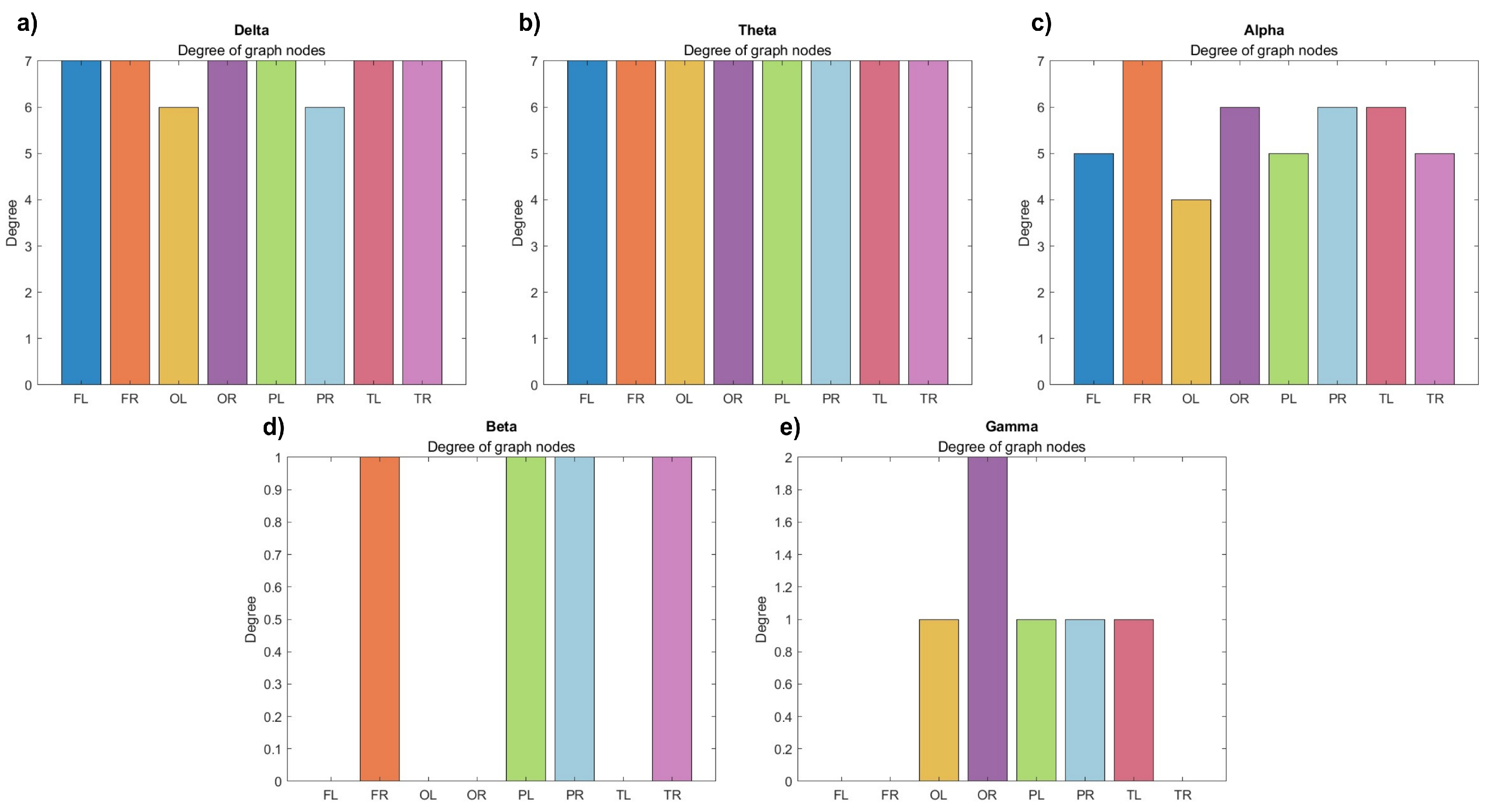
Figure 10.
Betweenness centrality for (a) delta, (b) theta, (c) alpha, (d) beta, and (e) gamma waves.
Figure 10.
Betweenness centrality for (a) delta, (b) theta, (c) alpha, (d) beta, and (e) gamma waves.
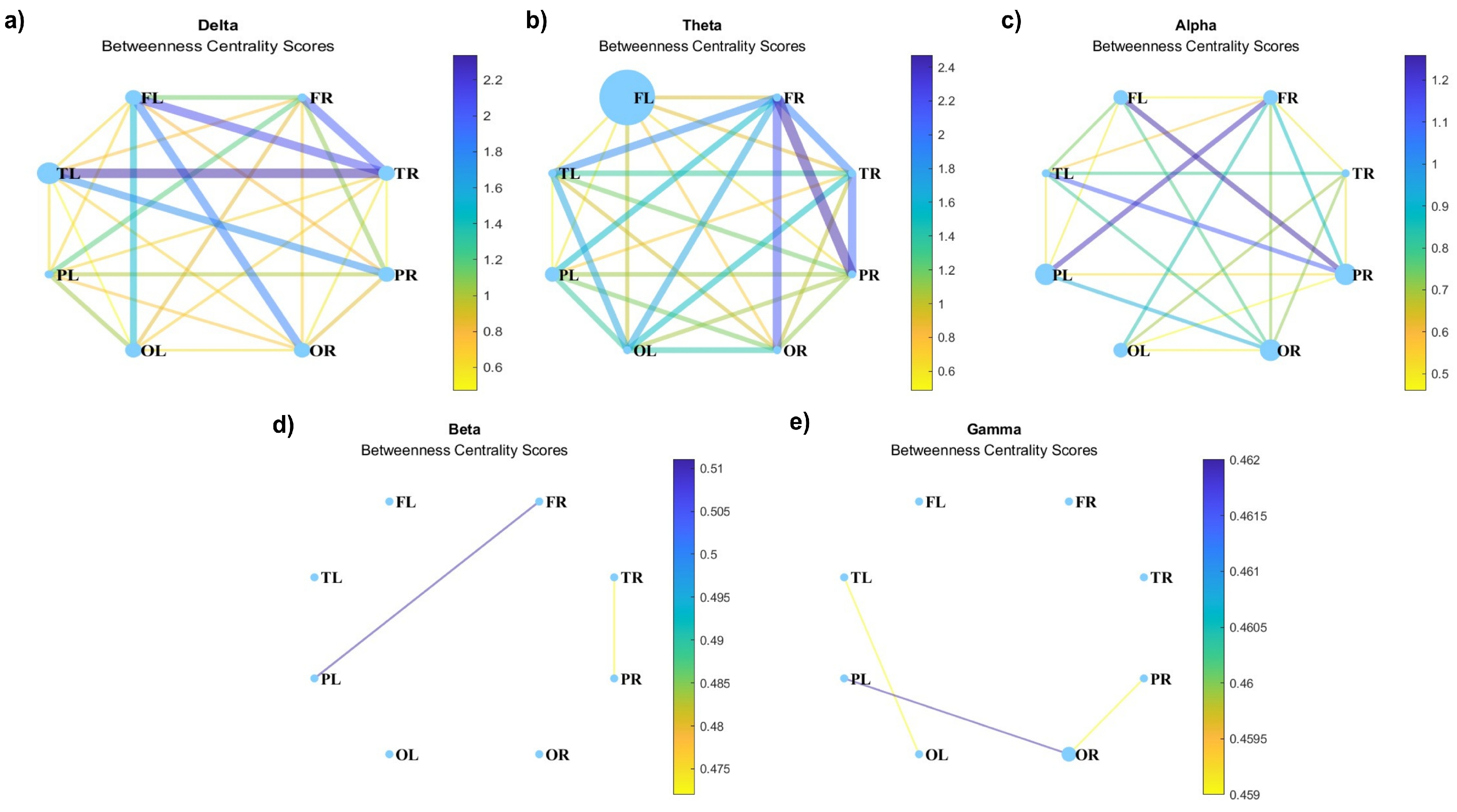
Figure 11.
Eigenvector centrality for (a) delta, (b) theta, (c) alpha, (d) beta, and (e) gamma waves.
Figure 11.
Eigenvector centrality for (a) delta, (b) theta, (c) alpha, (d) beta, and (e) gamma waves.
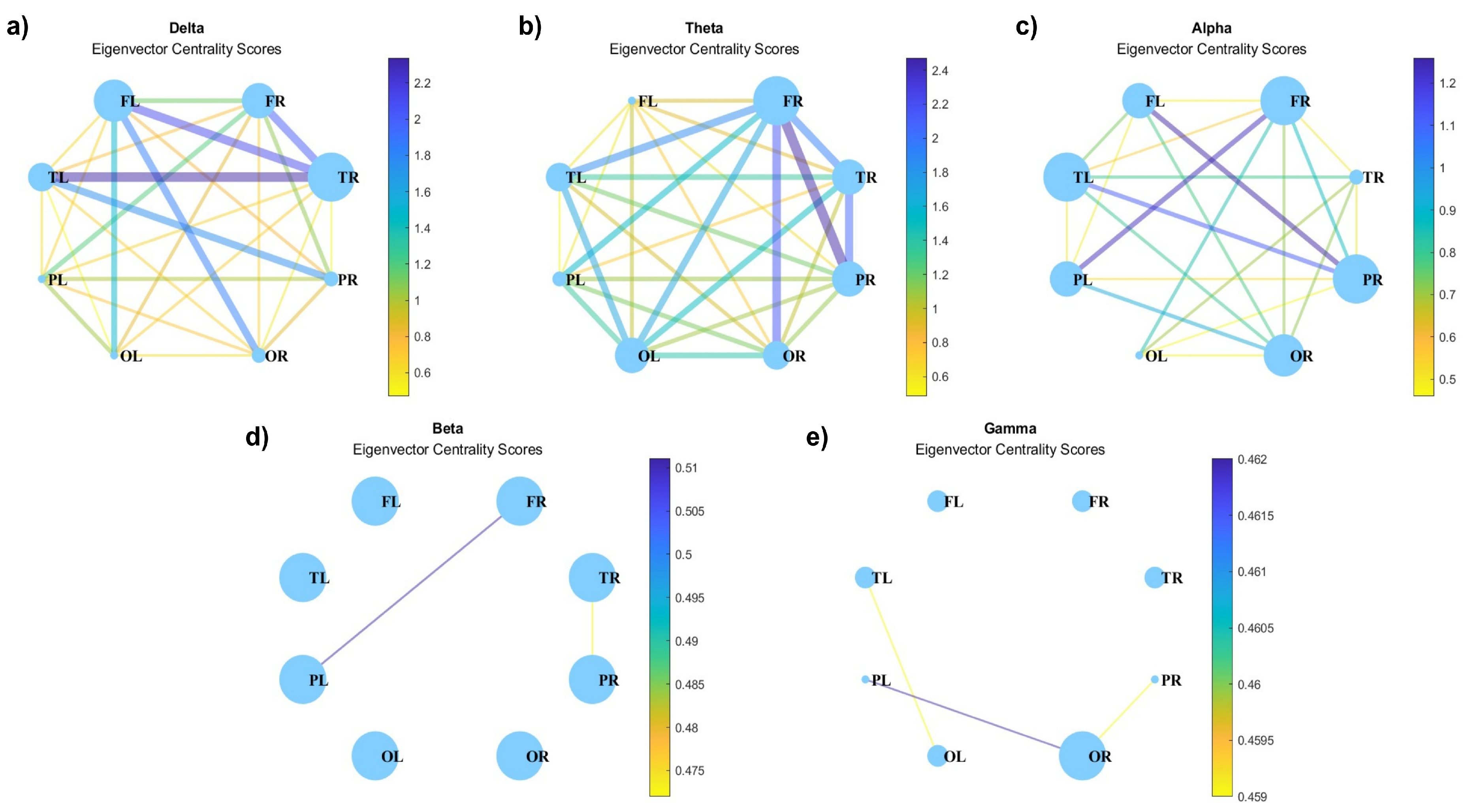
Figure 12.
Connected graph components for (a) delta, (b) theta, (c) alpha, (d) beta, and (e) gamma waves. Right frontal lobe (FR), Left frontal lobe (FL), Right parietal lobe (PR), Left parietal lobe (PL), Right temporal lobe (TR), Left temporal lobe (TL), Right occipital lobe (OR), Left occipital lobe (OL).
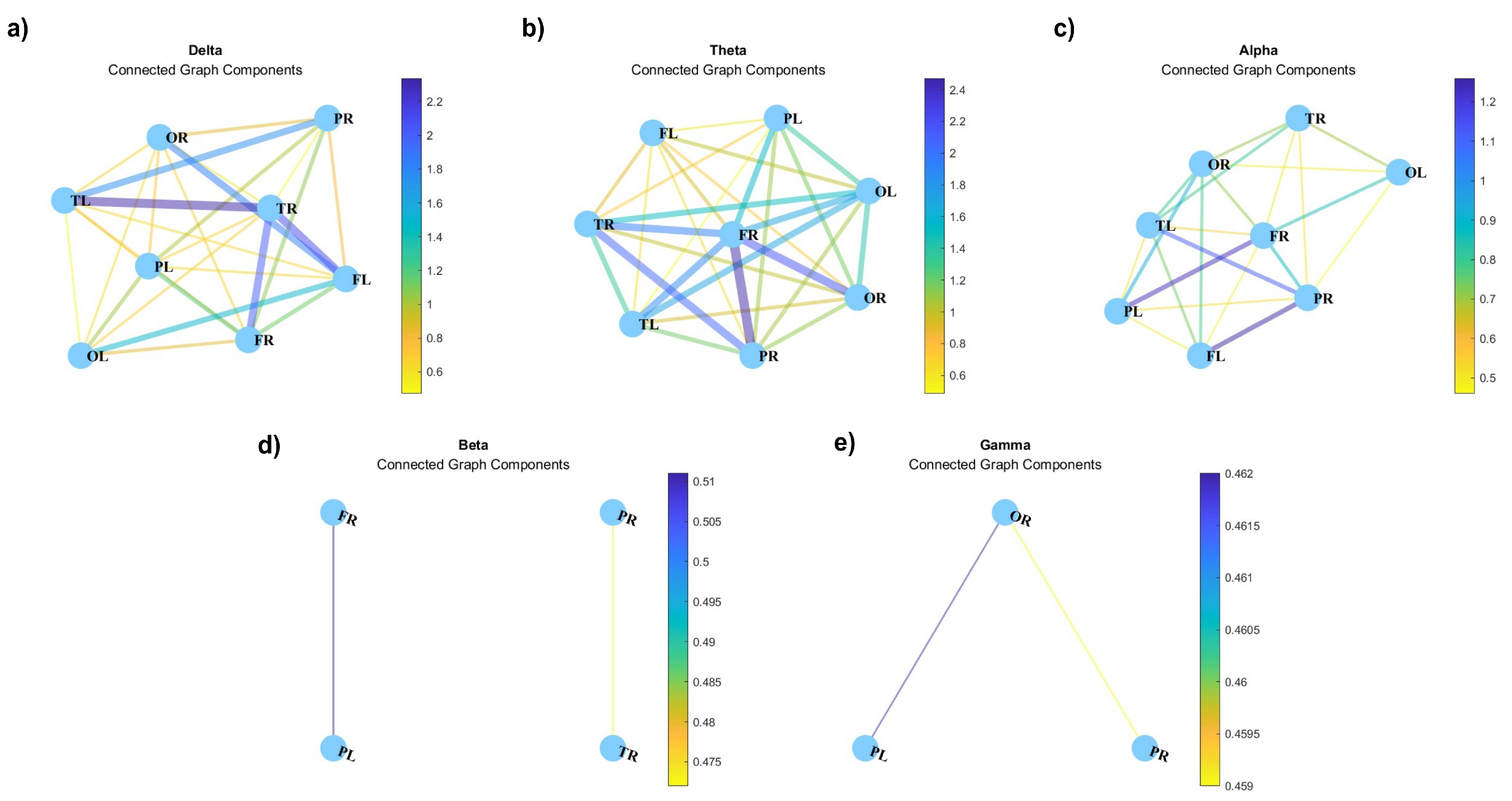
Figure 13.
Cycles of the graphs for (a) delta, (b) theta, and (c) alpha waves.
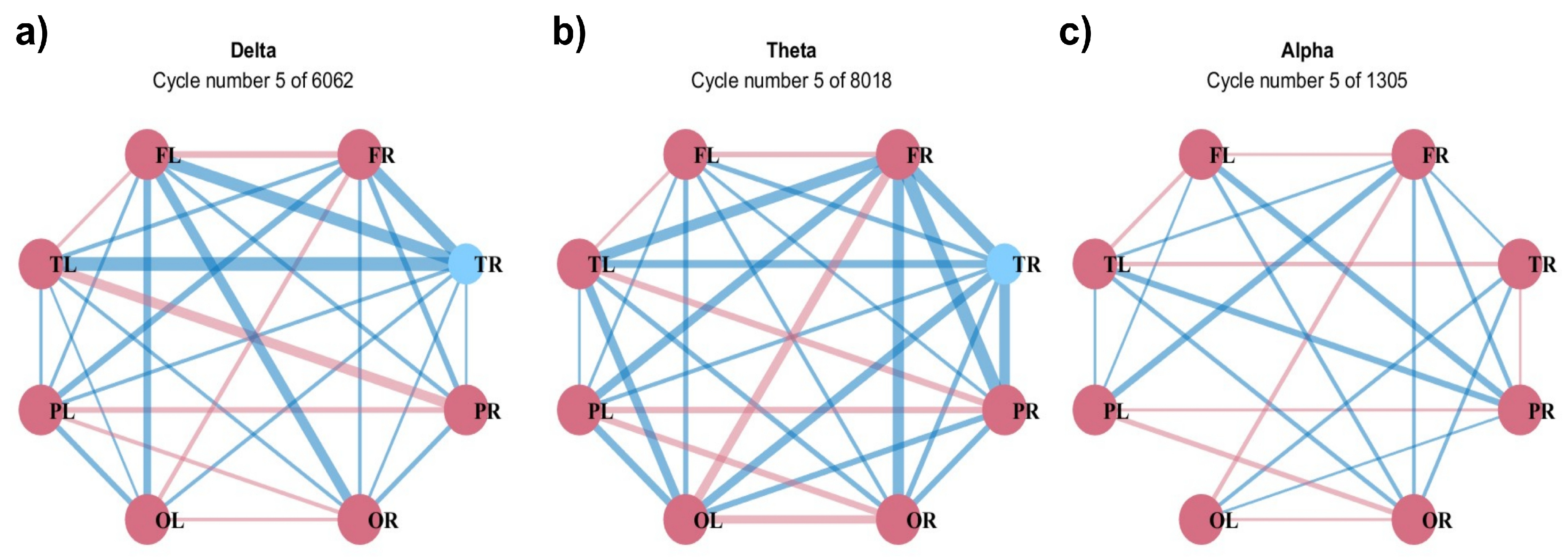
Figure 14.
Hypergraph representation as (a) network, (b) star expansion, and (c) adjacency matrix.
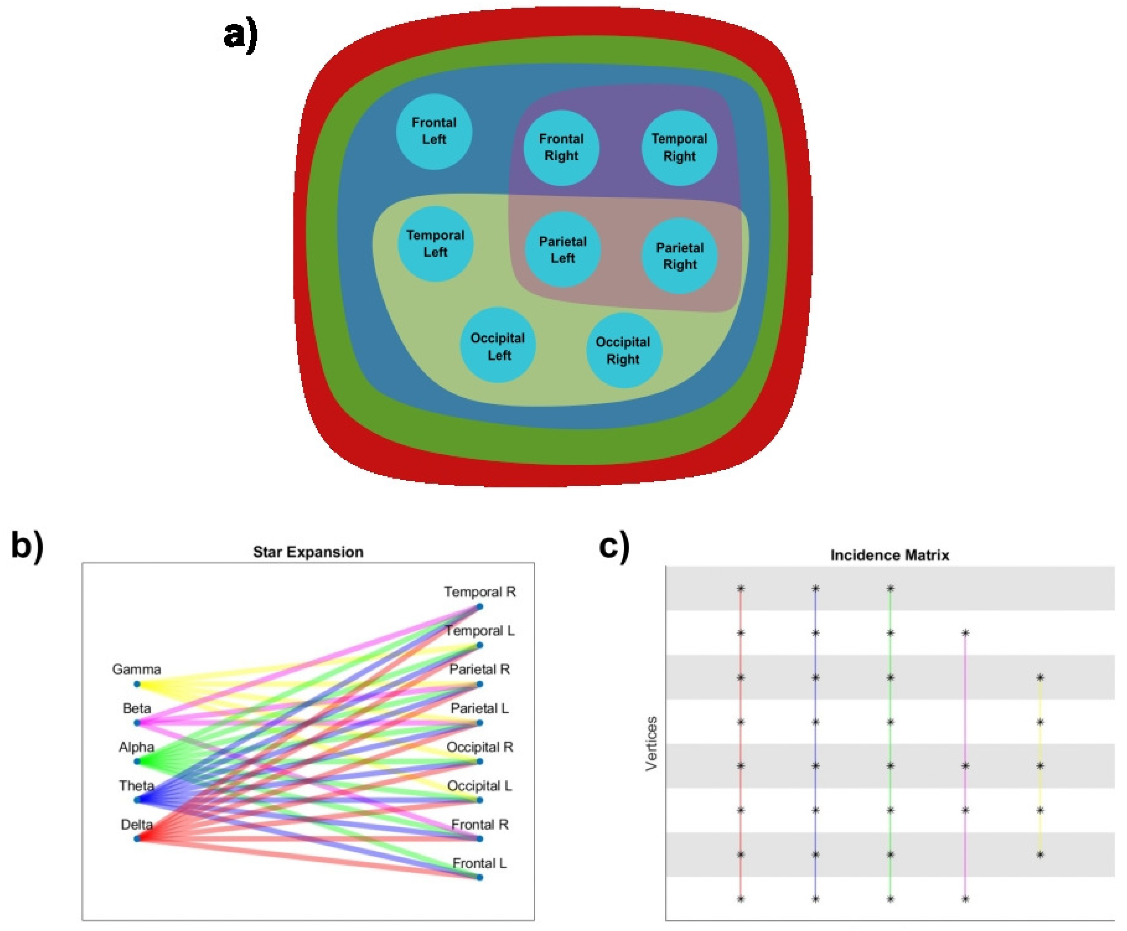
Figure 15.
2-section of the hypergraph.
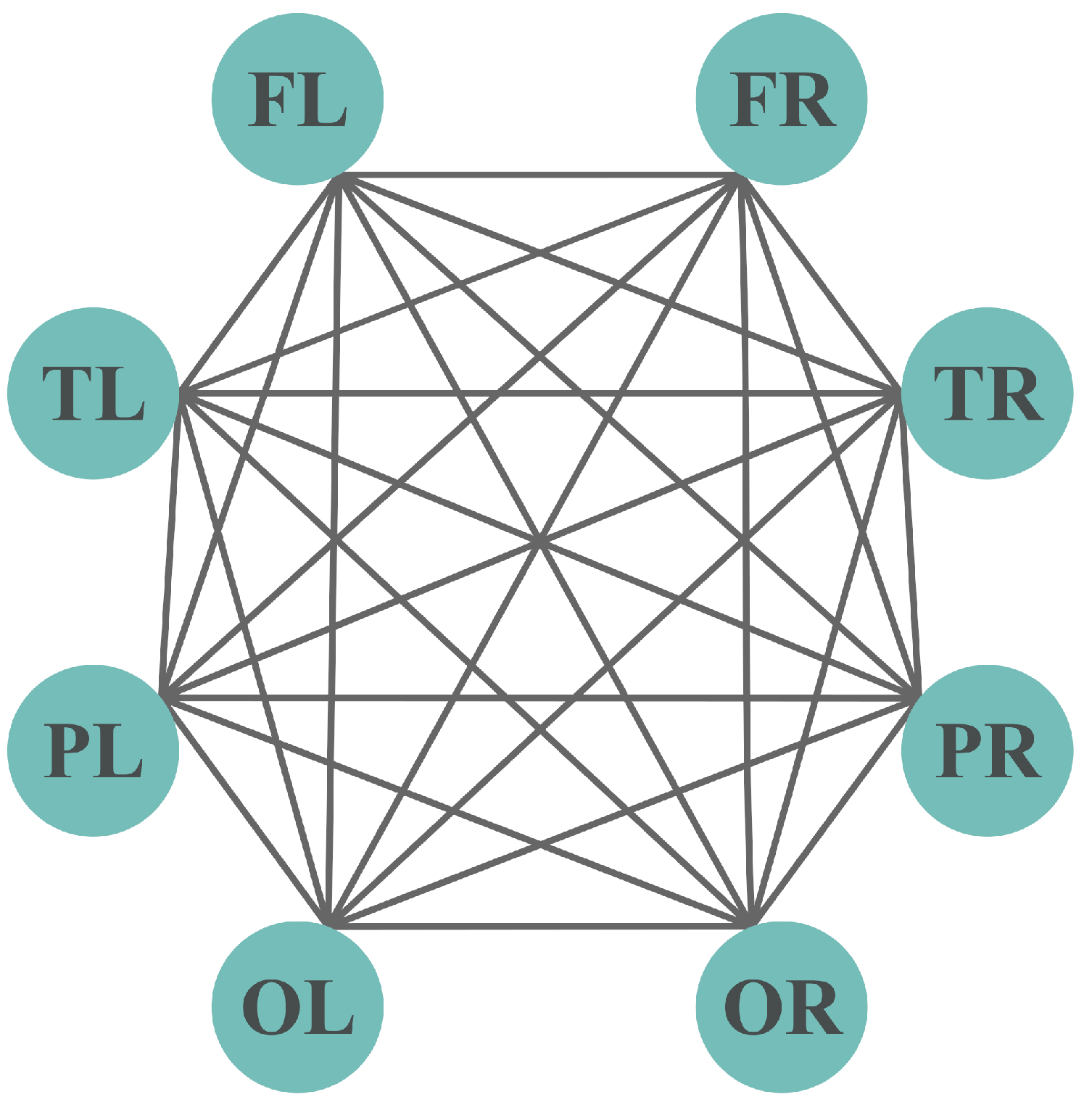
Figure 16.
Transversal of the hypergraph for delta (red), theta (blue), alpha (green), beta (magenta), and gamma (yellow) waves.
Figure 16.
Transversal of the hypergraph for delta (red), theta (blue), alpha (green), beta (magenta), and gamma (yellow) waves.
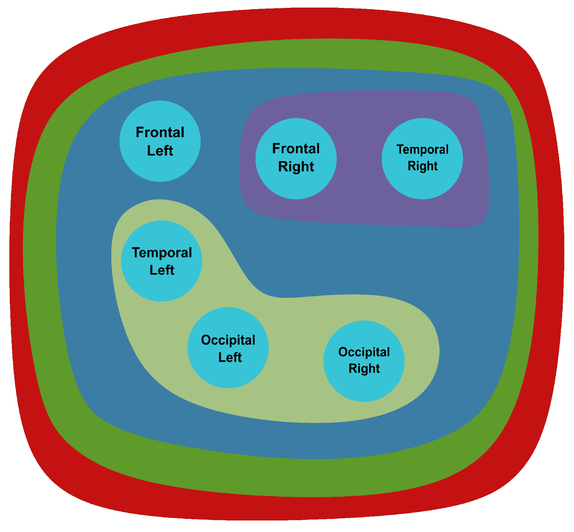
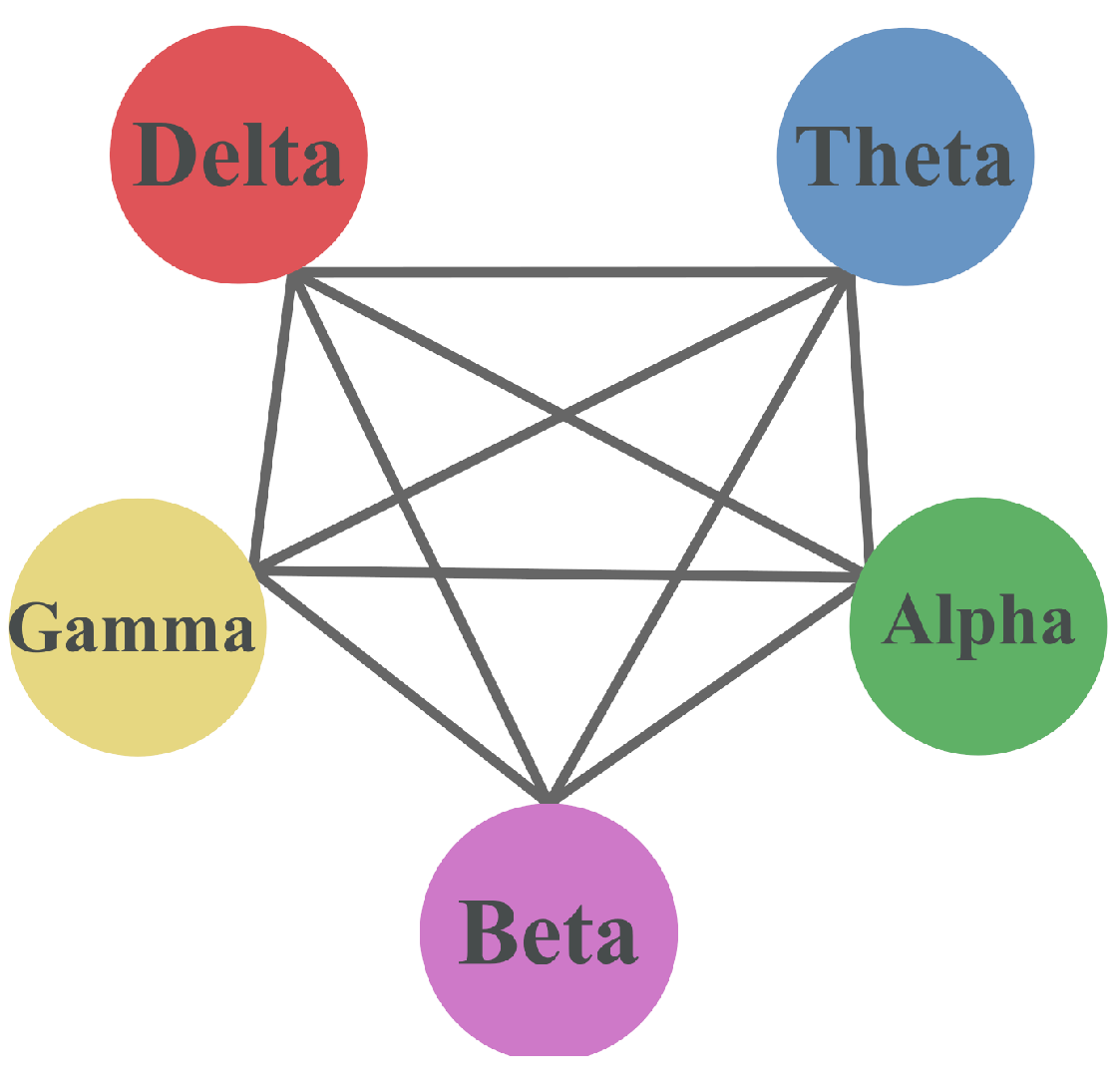
Figure 17.
Line graph.
Disclaimer/Publisher’s Note: The statements, opinions and data contained in all publications are solely those of the individual author(s) and contributor(s) and not of MDPI and/or the editor(s). MDPI and/or the editor(s) disclaim responsibility for any injury to people or property resulting from any ideas, methods, instructions or products referred to in the content. |
© 2024 by the authors. Licensee MDPI, Basel, Switzerland. This article is an open access article distributed under the terms and conditions of the Creative Commons Attribution (CC BY) license (http://creativecommons.org/licenses/by/4.0/).
Copyright: This open access article is published under a Creative Commons CC BY 4.0 license, which permit the free download, distribution, and reuse, provided that the author and preprint are cited in any reuse.


