Submitted:
22 January 2024
Posted:
24 January 2024
You are already at the latest version
Abstract
Marked changes in temperature, pH, dissolved oxygen (DO) content, and nutrient content typically occur in marine thermoclines, which are key factors that affect the corrosion of metals. Offshore platforms have required marine metals to be exposed to deep-sea environments and have thus increased their penetration into the marine thermocline. This study investigates the galvanic corrosion of E690 steel in a marine thermocline using a simulated marine thermocline (SMT). Specifically, the corrosion of E690 steel was analyzed using the wire beam electrode (WBE) technique, linear polarization (LP), corrosion morphology, and weight loss measurement. Results indicated that the SMT had a stable multilayer structure, and the variations of temperature, DO, pH and nutrient concentration in the SMT were similar to those in the natural marine thermocline. Galvanic corrosion occurred after the intrusion of E690 steel into the marine thermocline. The driver of galvanic corrosion was the of E690 steel at various depths of the marine thermocline. The Ecorr of E690 steel was influenced by the temperature, pH and DO of seawater, and the order was DO >> T > pH. The continuous reduction of Ecorr with depth contributed to the large-scale galvanic corrosion, and the oscillation variation of Ecorr with depth was the reason for small-scale galvanic corrosion. The primary anodic regions of galvanic corrosion were located in the area with the fastest temperature variation in the thermocline. The proportion of galvanic corrosion in the average corrosion rate could increase up to approximately 80% in the stable anodic region. There were many deep corrosion pits in the long-term and stable anodic region of galvanic corrosion.
Keywords:
Galvanic corrosion
; Simulated marine thermocline
; E690
; Dissolved oxygen
; Exploitation of ocean resource
1. Introduction
The basic three-layered structure (mixed layer, thermocline and abyssal layer) is typical of low- and mid-latitude seawater [1]. The marine thermocline is located at a water depth of nearly 30-150 m and exists all year in tropical and subtropical oceans [2]. The marine thermocline is described by features of high hydrostatic pressure and dramatic changes in the concentrations of DO, hydrogen ions (pH), and nutrients. The trend of marine resource development is to explore and extract resources from deeper water [3,4]. Offshore platforms are the most important devices in marine resource exploitation. E690 steel is a new type of high-strength-low-alloy bainite steel [5] that has good comprehensive mechanical properties and high application potential in marine engineering structures [6,7,8]. Many studies have been conducted on the corrosion fatigue and SCC (stress corrosion cracking) of E690 in a simulated marine environment [9]. E690 steel has high SCC susceptibility in marine environments due to the combined mechanism of AD (anodic dissolution) and HE (hydrogen embrittlement) [10]. Ma et al. [11,12,13] reported that SO2 in the marine atmosphere can facilitate the formation of a compact rust layer on the E690 steel surface, promoting the initiation of corrosion pits and reducing the toughness, and resulting in an increase in SCC susceptibility. Ma et al.[14] showed that the SCC susceptibility of E690 steel in simulated seawater was the lowest at approximately -850 mV/SCE and increased drastically when the potential was more negative than -950 mV/SCE. Although many studies have been performed on the corrosion of E690 steel in marine environments, most have focused on SCC and corrosion fatigue. Due to the influence of DO, water temperature, salinity, pH and dissolved inorganic nitrogen [15,16,17,18,19,20], the corrosion process of E690 steel is complex in marine environments. The corrosion of E690 steel is still not fully understood in seawater, particularly in the marine thermocline.
With the development of marine resource development, offshore platforms were built in “shallow water areas” for “deep water areas”. The steel piles of offshore platforms are more likely to suffer longitudinal non-uniform corrosion in the thermocline. The factors effecting corrosion and the corrosion mechanism of steel piles (E690 steel) are inconclusive, which might compromise the security of offshore platforms. The non-uniform corrosion of E690 steel in the marine thermocline is investigated in this study. A marine thermocline simulator (MTS) is designed and fabricated according to the formation mechanism of the marine thermocline to investigating E690 steel corrosion in the marine thermocline. Seawater taken from the South China Sea served as the electrolyte for the creation of an SMT. A removable and chain-type wire beam electrode (RCWBE) was used to understand the corrosion of the steel specimen. Electrochemical measurements (galvanic corrosion measurement technology, linear polarization), corrosion morphology observations and weight loss measurements were used to investigate the corrosion mechanism of E690 steel in SMT.
2. Experiment
2.1. Simulated marine thermocline
2.1.1. Marine thermocline simulator
Figure 1(a) shows a cross-section of the marine thermocline simulator (MTS). The MTS primarily includes four parts: a heat preservation bucket, temperature control unit, temperature measurement unit and sampling tube. The temperature control unit contains a water heater, cooling-water machine, warm water tank and cool water tank. The warm water tank was fixed at the top of the MTS, which was used to keep the upper part of the SMT at a relatively high temperature. The cool water tank was fixed at the bottom of the MTS, which was used to keep the lower part of the SMT at a relatively low temperature. The temperature measurement unit contains a multichannel thermometer and temperature sensor array. Figure 1(b) shows a cross-section of the sampling tube, which was used to take seawater samples for analysis.
2.1.2. Measurement of marine thermocline parameters
Seawater taken from the South China Sea served as the electrolyte for the SMT. Seawater was added to the heat preservation bucket before the MTS was operated.
A.Temperature measurement
The temperature measurement unit contains a multichannel thermometer and temperature sensor array. The temperature sensors were numbered 1 to 12 from bottom to top. The temperature data were collected every 10 minutes.
B. pH measurement
The SMT lasted for 66 days. On the 18th, 25th and 42nd days, seawater samples were taken through the sampling tube. The seawater sample pH was measured immediately by a pH values-3C pH meter with temperature compensation.
C.Measurement of DO and nutrient contents
The DO and nutrient (nitrate, phosphate and silicate) contents of seawater samples were determined by a chemical method [21] on the 18th, 25th and 42nd days.
2.2. Material
The E690 steel used in this study was produced by China Baowu Steel Group Corporation Limited, whose microstructure was lath-like bainite. The chemical compositions of E690 steel are shown in Table 1. The E690 steel was cut into specimens, which were 4 mm thick and 39 mm diameter discs. The specimens were gradually ground down to 1000 grid with SiC paper, degreased with acetone and rinsed with deionized water.
A removable-and-chain-type wire beam electrode (RCWBE) [22] was used to understand the corrosion of the steel specimen with the aid of the wire beam electrode (WBE) technique. The RCWBE was used to simulate the long metal in the SMT and consisted of many individual electrodes with an adjacent separation of 15 cm. The individual electrode was fabricated from an E690 steel specimen, rubber ring, PVC screw, and wires. Figure 2(a) and (b) show the two types of RCWBE in response to purpose, “A” used for electrochemical measurements and “B” for morphology observation and corrosion weight loss rate measurements, respectively.
2.3. Corrosion research method
The RCWBEs were vertically placed in the SMT, where the bottom single electrodes were 10 cm above the bottom section. The single electrode and corresponding temperature measurement point and corresponding sampling point were located at the same cylindrical surface.
2.3.1. Marine thermocline simulator
In situ measurements of the galvanic currents were performed on the 1st, 7th, 14th, 20th, 27th, 44th and 59th days. Galvanic currents of the RCWBEs were measured by the electrochemical noise (ECN) method via a PGSTAT302N AUTOLAB potentiostat and NOVA1.11 software. Two work electrodes (W1, W2) and one reference electrode, the saturated calomel electrode (SCE), were considered as the ECN measurement. A single electrode of one column of RCWBE was connected with W1, while the other electrodes of the same column were simultaneously connected with W2. The ECN of every single electrode was measured for 30 s, and then, the electrodes connected with W1 and W2 were replaced. Then, the ECN of the entire RCWBE was measured, and the galvanic current of each electrode of the array was determined from the analyzed ECN data [22,23] .
2.3.2. Measurement of instantaneous Icorr and Ecorr
In situ measurements for linear polarization (LP) were performed on the 1st, 7th, 14th, 20th, 27th, 44th and 59th days. The single electrodes were each subjected to LP on a three-electrode cell, which comprised a single electrode as the working electrode, a 2 × 2 cm2 Pt plate as the counter electrode, and an SCE as the reference electrode. The LP curves were measured via potential scanning from -10 to +10 mV against open-circuit potentials at a rate of 0.00167 mV/s. Instantaneous values of each electrode Icorr and Ecorr were obtained from the analysis of the LP data.
2.3.3. Corrosion morphology observation
The B-type RCWBEs were removed from the MTS on the 10th, 23rd, 32nd, 41st, 51st and 66th days, and then observed via a HITACHI TM4000 Plus SEM, three-dimensional microscope and camera. After derusting and drying, each electrode was observed again.
2.3.4. wt loss measurement
Pre-weighed E690 steel specimens were installed in the B-type RCWBEs and then immersed in the simulated thermocline. After morphological observation of the specimens, they were cleaned with acetone and reweighed. The wt loss data were calculated by the formula given in Eq. (1):
Where V is the average corrosion rate, mm/y; W0 is the initial weight of the E690 specimen, g; W1 is the weight of the derusted E690 specimen, g; A is the exposure area of the E690 specimen, cm2; t is the exposure time, hour; and ρ is the density of the metal, g/cm3.
3. Results and discussion
3.1. Characterization of the simulated marine thermocline
The temperature measurement points and sampling points were numbered 1 to 12 from bottom to top, respectively. Seawater at room temperature was added to the heat preservation bucket before the MTS was operated. The entire experiment lasted for 66 days, and the temperature data were collected every 10 minutes. On the 18th, 25th and 42nd days, seawater samples at different depths were removed through the sampling pipe, and the pH, DO and nutrient content were measured.
3.1.1. Temperature variation in the simulated marine thermocline
Figure 3 shows the longitudinal temperature variation of the SMT. From the 0th to the 7th day, the temperature at the bottom points changed markedly. A stable and strong temperature gradient first appeared on the 7th day and lasted until the 66th day. After the 7th day, the multilayer structure of seawater formed and remained stable. The temperature of the upper seawater layer was 32 °C, and that of the lower seawater layer was 12 °C. The range of temperature variation in the SMT was similar to that in the marine thermocline in the northern area of the South China Sea in summer.
3.1.2. Components variation of simulated marine thermocline
Figure 4 shows the component variations of SMT. On the 18th day, the DO increased with increasing seawater depth. The DO of the upper layer seawater decreased from 1.09 mg/L on the 18th day to 0.42 mg/L on the 25th day. The DO of the bottom seawater decreased from 5.60 mg/L to 0.24 mg/L. The DO decreased with increasing seawater depth on the 25th and 42nd days. The DO variation of SMT showed a stable multilayer structure formation. There is a small quantity of biodetritus in natural seawater. As shown in reaction (1), the biodetritus slowly decomposed into inorganic substances and simultaneously consumed DO. The decomposition reaction of biodetritus is influenced by temperature. Before the 18th day, the DO consumption rate in the warm and upper seawater was higher than that in the cool and bottom seawater. The O2 transmission is subject to the stable multilayer structure of the thermocline:
The seawater pH increased with increasing seawater depth and decreased with time. As in reaction (1), CO2 and H+ were produced in the biodetritus decomposition process. The decomposition rate of biodetritus in the warm and upper seawater was higher than that in the cool and bottom seawater:
Reaction 1 is the decomposition reaction of biodetritus in oxygen-enriched seawater, and reaction 2 is that in oxygen-poor seawater. biodetritus decomposition caused the nitrate concentration in the initial and high DO stages of the thermocline to increase. With dwindling DO levels, the nitrate concentration decreased for the biodetritus decomposition, as in reaction 2. The concentration changes of phosphate and silicate were influenced by the biodetritus decomposition and pH variation.
Considering all of these results, the SMT was a stable multilayer structure, and the variation rules of temperature, DO, pH and nutrient concentration in the SMT were similar to those in the natural marine thermocline.
3.2. Galvanic corrosion of E690 offshore platform steel in a simulated marine thermocline
Figure 5 shows the variation in the galvanic current (Ig) of WBEs in the SMT. The maximum Ig increased with experimental time from the 7th day to the 44th day, and then, the maximum Ig decreased on the 59th day. From the longitudinal temperature variation of SMT, the primary anodic regions were located in the fastest temperature variation area, and the position of the primary anodic region rose with time. The anodic region was intermixed with the cathodic region on the 59th day and in the lower part of the SMT.
3.3. Driver of E690 offshore platform steel galvanic corrosion in SMT
The Ecorr of single electrodes were measured by in situ linear polarization measurements. Figure 6(a) describes all Ecorr of E690 steel in the simulated thermocline. The Ecorr of a single electrode at a depth of 75 cm changes with time, as shown in Figure 6(b). The Ecorr markedly decreased from -0.519 V vs. SCE on the 1st day to -0.727 V on the 14th day and then gradually increased with time. The electrochemical corrosion reaction of steel (see reactions 3-5) and the Nernst equation (see Equation 7) showed that the Ecorr of steel was influenced by the temperature, pH and DO of seawater. Comparing the Ecorr variation and marine thermocline component variation, Ecorr was most affected by DO; this result was supported by the macrocorrosion morphology of rusted E690 specimens (see Table 2). Due to the high concentration of DO, the color of the E690 corrosion products was yellowish on the 7th day (i.e., the principle in reaction 6). The color of the E690 corrosion products changed from yellowish high-valence iron compounds to taupe low-valence iron compounds with time and depth. For the small variation in pH in the simulated thermocline, the Ecorr was marginally affected by pH. The Ecorr of E690 steel was influenced by the temperature, pH and DO of seawater in the simulated thermocline, and the order was DO >> T > pH.
If a long piece of steel leads through the marine thermocline, the driver of galvanic corrosion of steel is the of steel at various depths. As shown in Figure 6(c), the continuous reduction of Ecorr with depth contributed to large-scale galvanic corrosion, and the oscillation variation of Ecorr with depth was the reason for small-scale galvanic corrosion:
Negative electrode reaction:
Positive electrode reaction:
Total reaction equation:
Oxygen-enriched seawater environment:
According to the Nernst equation:
: real electrode potential; : standard electrode potential;
: the number of transferred electrons in the reaction equation;
: Faraday’s constant (96485 C·mol-1); : gas constant (8.314 J·K-1mol-1) ;
: temperature (K); : the partial pressure of O2;
: the concentration of (mol·L-1);
: the concentration of under normal conditions (mol·L-1)
3.3. Proportion of galvanic corrosion in E690 offshore platform steel corrosion
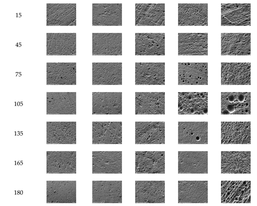
The average corrosion rates of E690 steel at the various depths of the SMT were measured via weight loss measurement. The “mm/y” of the average corrosion rate unit was converted into “μA/cm2”. Figure 7 shows a comparison of the galvanic current and average corrosion rate (weight loss rate). There were two forms of E690 steel corrosion in the SMT: galvanic corrosion and see-water corrosion. The see-water corrosion was the primary contributor of average corrosion. The see-water corrosion of E690 steel was influenced by DO (i.e., the principle in reaction 3-6). This result was supported by the average corrosion rate variation in Figure 7, the quantity variation of corrosion product in Table 3 and the variation rules of DO in Figure 4. In the anodic region of galvanic corrosion, the proportion of galvanic corrosion in the average corrosion rate first increased and then decreased. The proportion of galvanic corrosion in the average corrosion rate could increase up to approximately 80% in the anodic region. As shown in Table 4, there were many deep corrosion pits in the long-term and stable anodic region of galvanic corrosion.
4. Conclusions
Offshore platforms allow their seepage to develop in the deep sea, along with the penetration of a growing number of steel piles through the thermocline. To determine the scientific and practical value of galvanic corrosion in marine thermoclines, this study investigated the corrosion of E690 steel using a simulated seawater thermocline that was designed and fabricated by a developed RCWBE. The major findings of this first test study include the following:
- (1)
- The SMT was a stable multilayer structure. The variations of temperature, DO, pH and nutrient concentration in the SMT were similar to those in the natural marine thermocline.
- (2)
- Galvanic corrosion occurs after the intrusion of E690 steel into the marine thermocline. Primary anodic regions were located in the area with the fastest temperature variation, and the anodic region was intermixed with the cathodic region in the lower part of the stable marine thermocline.
- (3)
- The driver of galvanic corrosion of E690 steel in the marine thermocline was the of E690 steel at various depths. The continuous reduction of Ecorr with depth contributed to the large-scale galvanic corrosion, and the oscillation variation of Ecorrwith depth was the reason for small-scale galvanic corrosion.
- (4)
- The Ecorr of E690 steel was influenced by the temperature, pH and DO in the marine thermocline, and the order was DO >> T > pH.
- (5)
- There were at least two forms of E690 steel corrosion in the marine thermocline: galvanic corrosion and see-water corrosion. The proportion of galvanic corrosion in the average corrosion rate could increase up to approximately 80% in the anodic region. There were many deep corrosion pits in the long-term and stable anodic region of galvanic corrosion.
Author Contributions
Conceptualization, J.H. and P.D.; methodology, P.D.; software, Y.T.; validation, J.H., G.L. and Z.L.; formal analysis, J.H.; investigation, Z.L.; resources, J.H. and P.D.; data curation, G.L.; writing—original preparation, J.H. and G.L.; writing—review and editing, P.D.; visualization, Y.T. and Z.L.; supervision, P.D.; project administration, Y.T.; funding acquisition, J.H. and P.D. All authors have read and agreed to the published version of the manuscript.
Funding
This research was funded by Natural Science Foundation of China (51801033), Natural Science Foundation of Guangdong Province China (2021A1515110382) and Science & Technology Development Fundation of Zhanjiang (2022A01029).
Data Availability Statement
Not applicable.
Acknowledgments
The authors were sincerely grateful for the financial support from Natural Science Foundation of China (51801033), Natural Science Foundation of Guangdong Province China (2021A1515110382) and Science & Technology Development Fundation of Zhanjiang (2022A01029).
Conflicts of Interest
The authors declare that they have no known competing financial interests or personal relationships that could have appeared to influence the work reported in this paper.
References
- Lynne D.T.; Pickard, G.L. Typical Distributions of Water Characteristics. Descriptive physical oceanography: an introduction, 6th ed.; Elsevier, London, 2011; 67-110.
- Zhang, X.; Prange, M. Changes in equatorial Pacific thermocline depth in response to Panamanian seaway closure: Insights from a multi-model study. Earth Planet Sci. Lett. 2012, 317, 76–84. [Google Scholar] [CrossRef]
- Dehghani, A.; Aslani, F. A review on defects in steel offshore structures and developed strengthening techniques. Structures. 2019, 20, 635–657. [Google Scholar] [CrossRef]
- Saiful Islam, A.B.M.; Jameel, M. Review of offshore energy in Malaysia and floating Spar platform for sustainable exploration. Renewable Sustainable Energy Rev. 2012, 16, 6268–6284. [Google Scholar] [CrossRef]
- Li, Y.; Liu, Z. Effect of cathodic potential on stress corrosion cracking behavior of different heat-affected zone microstructures of E690 steel in artificial seawater. J. Mater. Sci. Technol. 2021, 64, 141–152. [Google Scholar] [CrossRef]
- Liu, Z.; Hao, W. Fundamental investigation of stress corrosion cracking of E690 steel in simulated marine thin electrolyte layer. Corros. Sci. 2019, 148, 388–396. [Google Scholar] [CrossRef]
- Ma, H.C.; Fan, Y. Effect of pre-strain on the electrochemical and stress corrosion cracking behavior of E690 steel in simulated marine atmosphere. Ocean Eng. 2019, 182, 188–195. [Google Scholar] [CrossRef]
- Ma, H.C.; Liu, Z.Y. Stress corrosion cracking of E690 steel as a welded joint in a simulated marine atmosphere containing sulphur dioxide. Corros. Sci. 2015, 100, 627–641. [Google Scholar] [CrossRef]
- Lu, Q.; Wang, L. Corrosion evolution and stress corrosion cracking of E690 steel for marine construction in artificial seawater under potentiostatic anodic polarization. Constr. Build. Mater. 2020, 238, 117763. [Google Scholar] [CrossRef]
- Tian, H.; Wang, X. Electrochemical corrosion, hydrogen permeation and stress corrosion cracking behavior of E690 steel in thiosulfate-containing artificial seawater. Corros. Sci. 2018, 144, 145–162. [Google Scholar] [CrossRef]
- Ma, H.; Liu, Z. Comparative study of the SCC behavior of E690 steel and simulated HAZ microstructures in a SO2-polluted marine atmosphere. Mater. Sci. Eng., A. 2016, 650, 93–101. [Google Scholar] [CrossRef]
- Ma, H.; Du, C. Effect of SO2 content on SCC behavior of E690 high-strength steel in SO2-polluted marine atmosphere. Ocean Eng. 2018, 164, 256–262. [Google Scholar] [CrossRef]
- Ma, H.; Chen, L. Effect of prior austenite grain boundaries on corrosion fatigue behaviors of E690 high strength low alloy steel in simulated marine atmosphere. Mater. Sci. Eng., A. 2020, 773, 138884. [Google Scholar] [CrossRef]
- Ma, H.; Liu, Z. Effect of cathodic potentials on the SCC behavior of E690 steel in simulated seawater. Mater. Sci. Eng., A. 2015, 642, 22–31. [Google Scholar] [CrossRef]
- Gardiner, C.P.; Melchers, R.E. Corrosion analysis of bulk carriers, Part I: operational parameters influencing corrosion rates. Mar. Struct. 2003, 16, 547–566. [Google Scholar] [CrossRef]
- Melchers, R.E. Effect of small compositional changes on marine immersion corrosion of low alloy steels. Corros. Sci. 2004, 46, 1669–1691. [Google Scholar] [CrossRef]
- Melchers, R.E.; Jeffrey, R. Early corrosion of mild steel in seawater. Corros. Sci. 2005, 47, 1678–1693. [Google Scholar] [CrossRef]
- Robert, E. Melchers, Robert Jeffrey. 2012. Corrosion of long vertical steel strips in the marine tidal zone and implications for ALWC. Corros. Sci. 2012, 65, 26–36. [Google Scholar]
- Traverso, P.; Canepa, E. A review of studies on corrosion of metals and alloys in deep-sea environment. Ocean Eng. 2014, 87, 10–15. [Google Scholar] [CrossRef]
- Wall, H.; Wadsö, L. Corrosion rate measurements in steel sheet pile walls in a marine environment. Mar. Struct. 2013, 33, 21–32. [Google Scholar]
- Committee, C.N.S.M. GB/T 12763.4-2007, in Code for marine surveys Part 4 Investigation of seawater chemical elements. 2008, China Standard Press: Beijing.
- Deng, P.; Li, Z. Vertical galvanic corrosion of pipeline steel in simulated marine thermocline. Ocean Eng. 2020, 217, 107584. [Google Scholar]
- Hu, J.; Deng, P. The vertical Non-uniform corrosion of Reinforced concrete exposed to the marine environments. Constr. Build. Mater. 2018, 183, 180–188. [Google Scholar] [CrossRef]
Figure 1.
Cross-section image of the marine thermocline simulator.
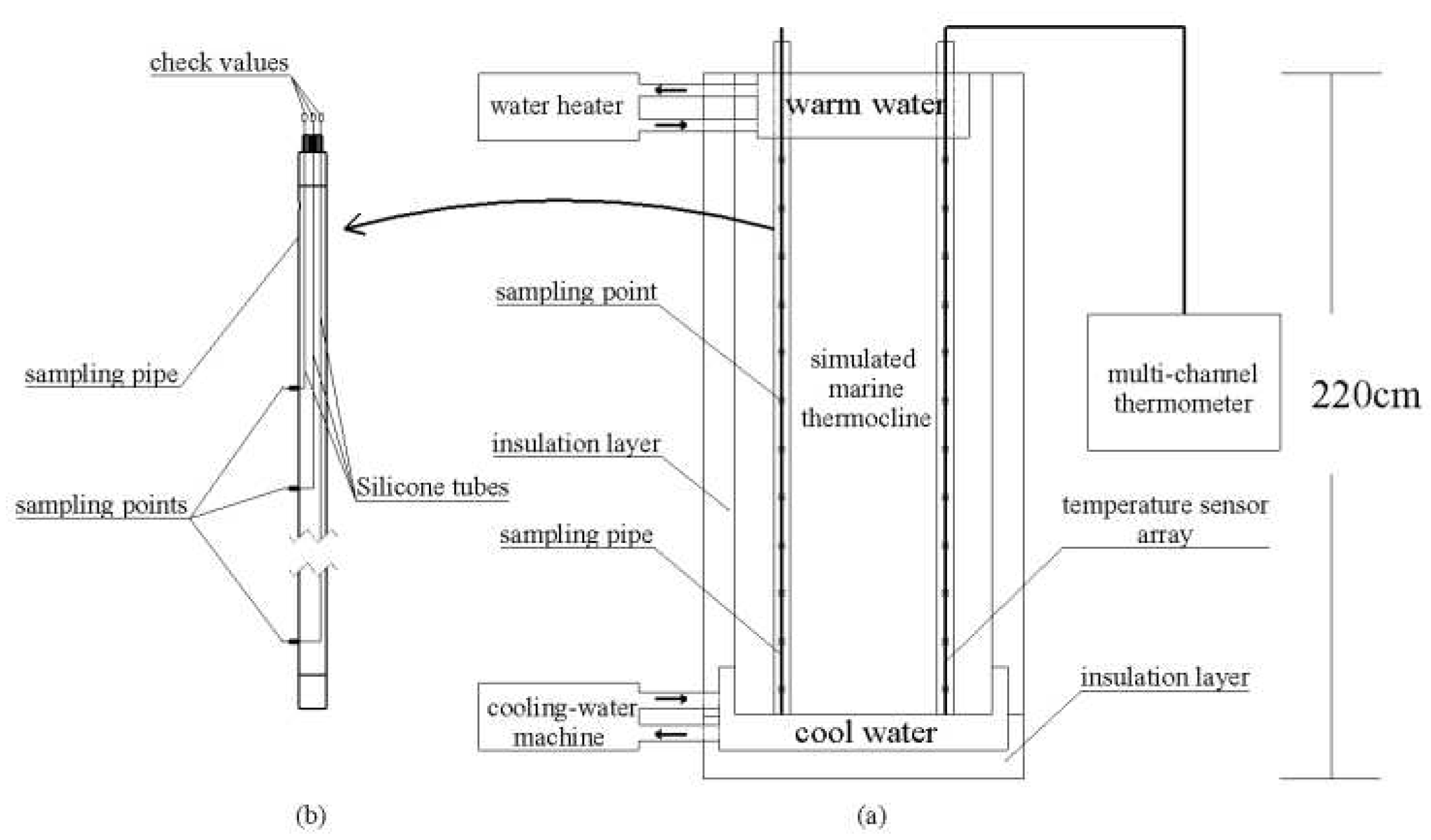
Figure 2.
Connection mode of RCWBE.
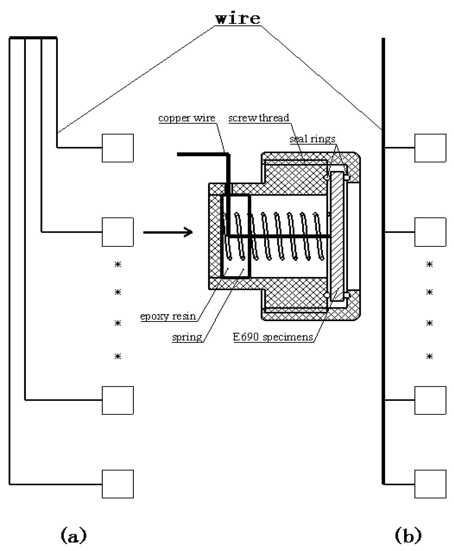
Figure 3.
Longitudinal variation of temperature in simulated marine thermocline.

Figure 4.
Evolution of simulated marine thermocline structure: 18th day; B. 25th day; C. 42th day).
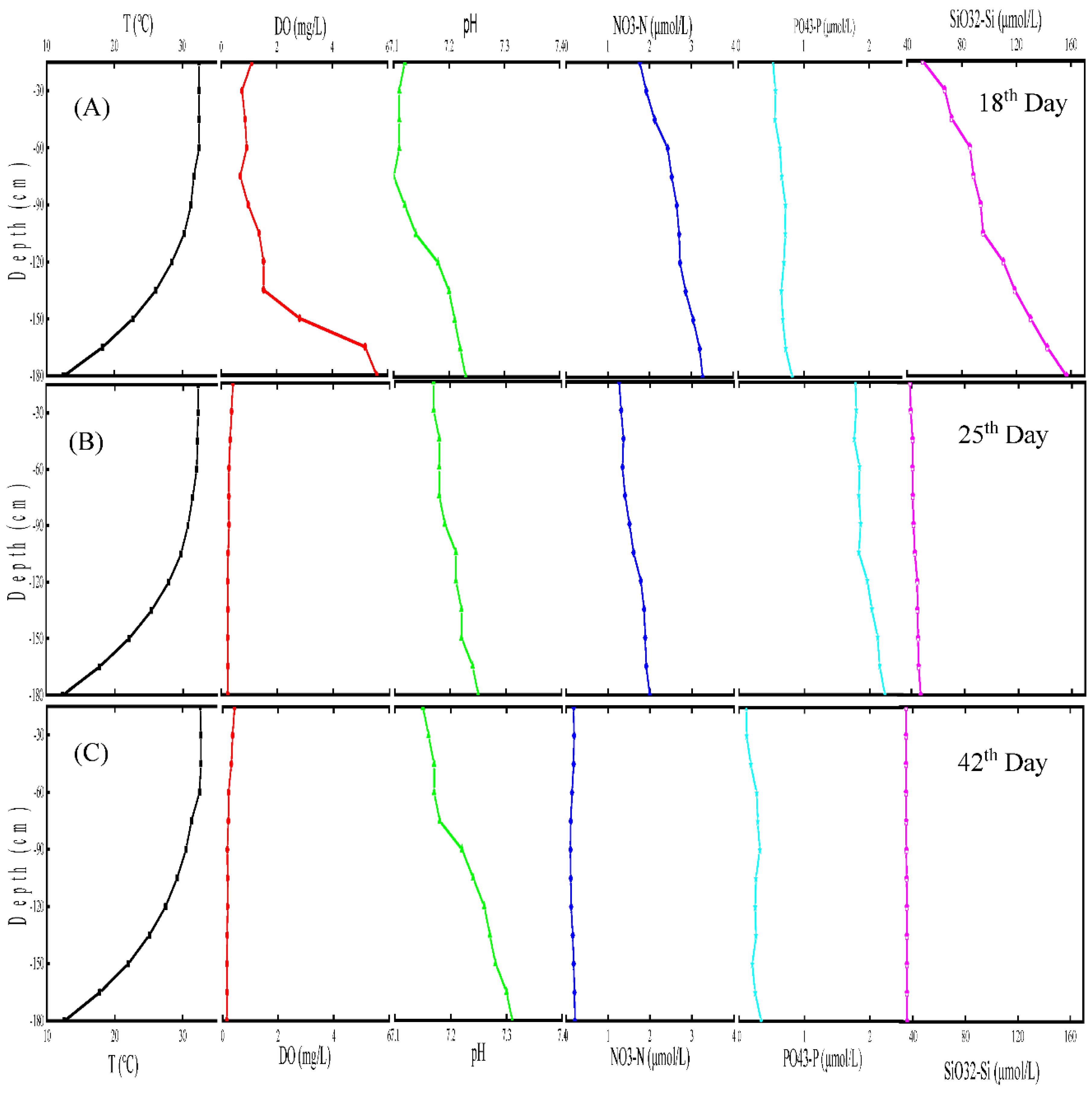
Figure 5.
Variation of galvanic current of RCWBE in the SMT.
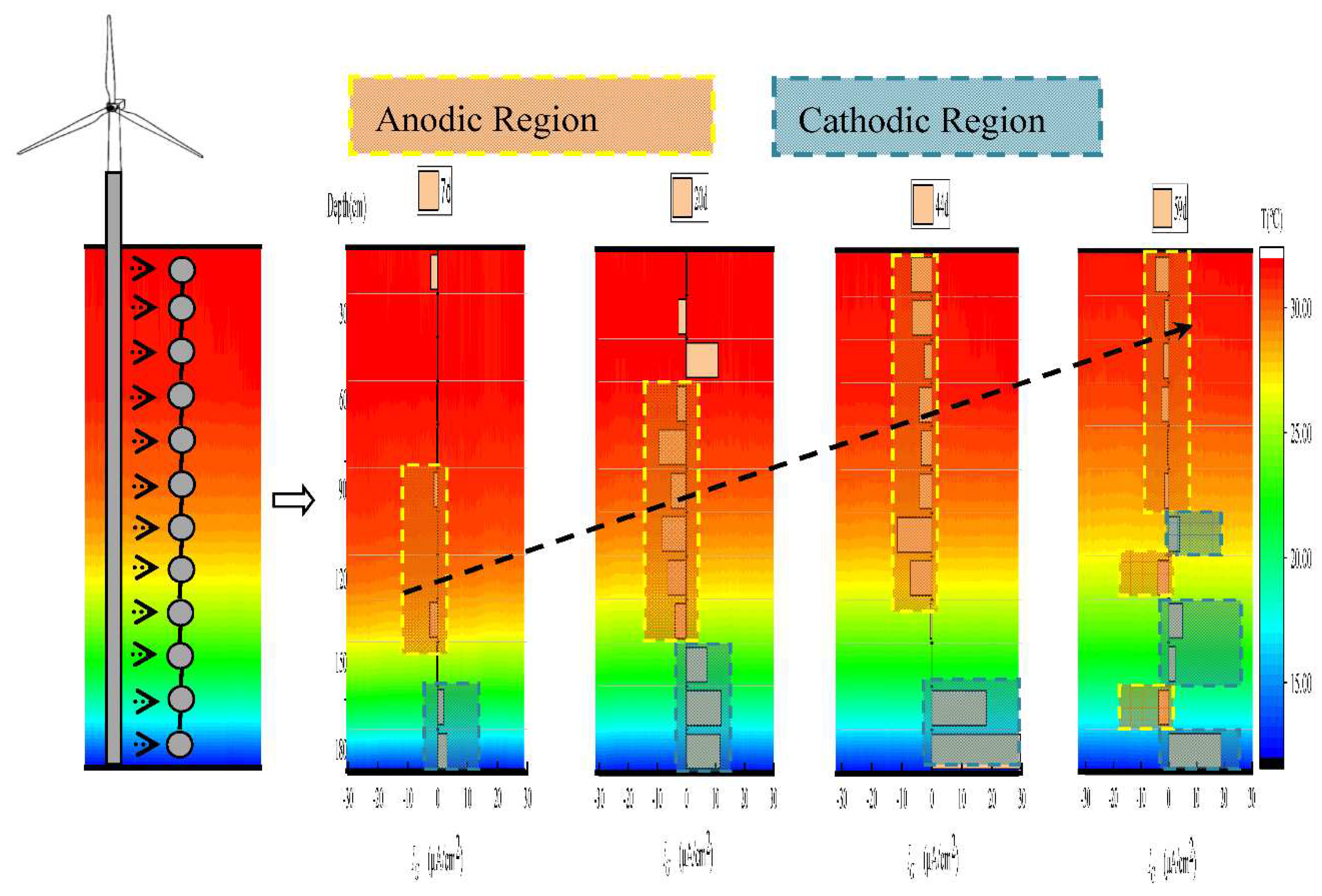
Figure 6.
Variation of E690 steel Ecorr in the simulated thermocline.
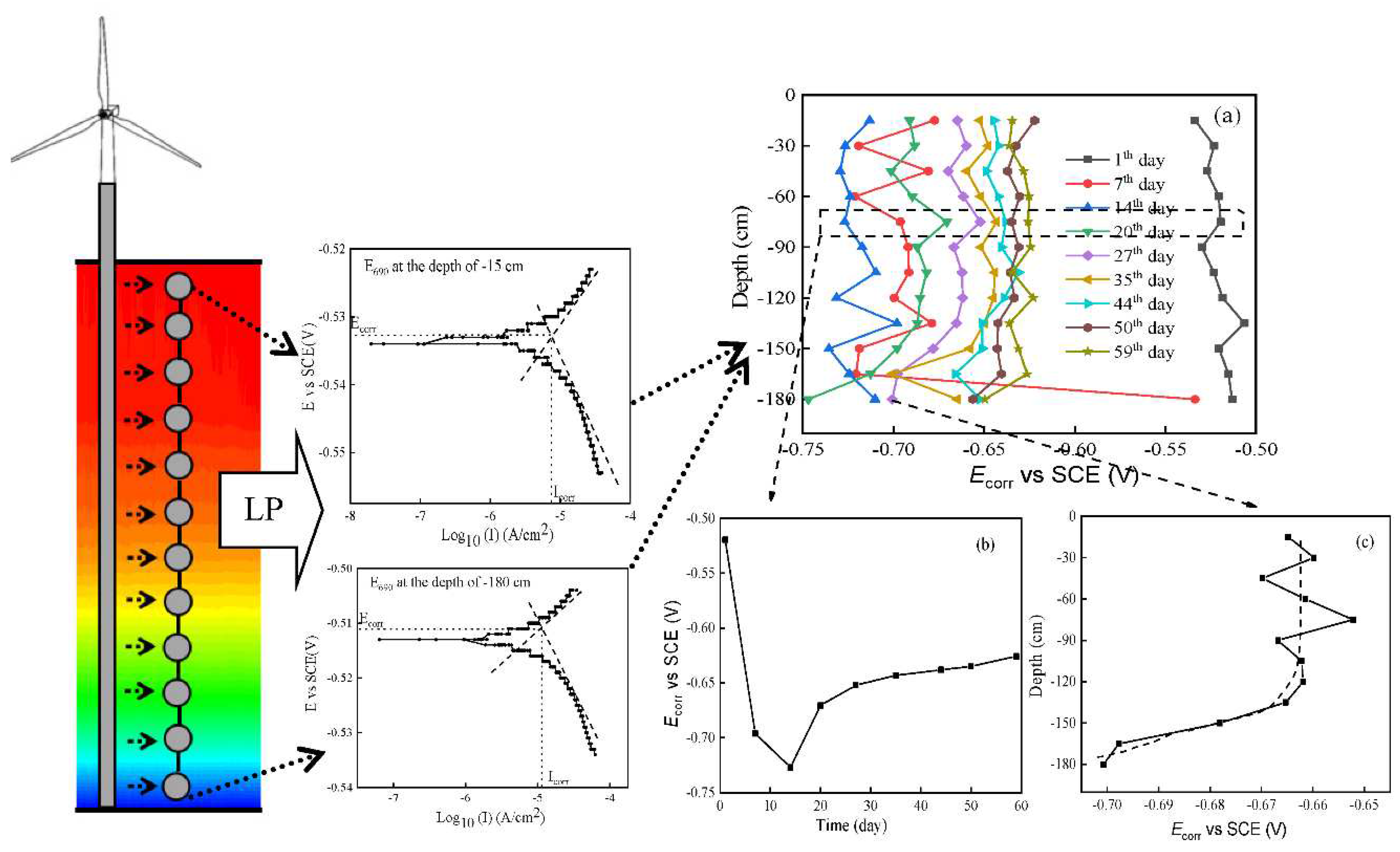
Figure 7.
the comparison of galvanic current and average corrosion rate.
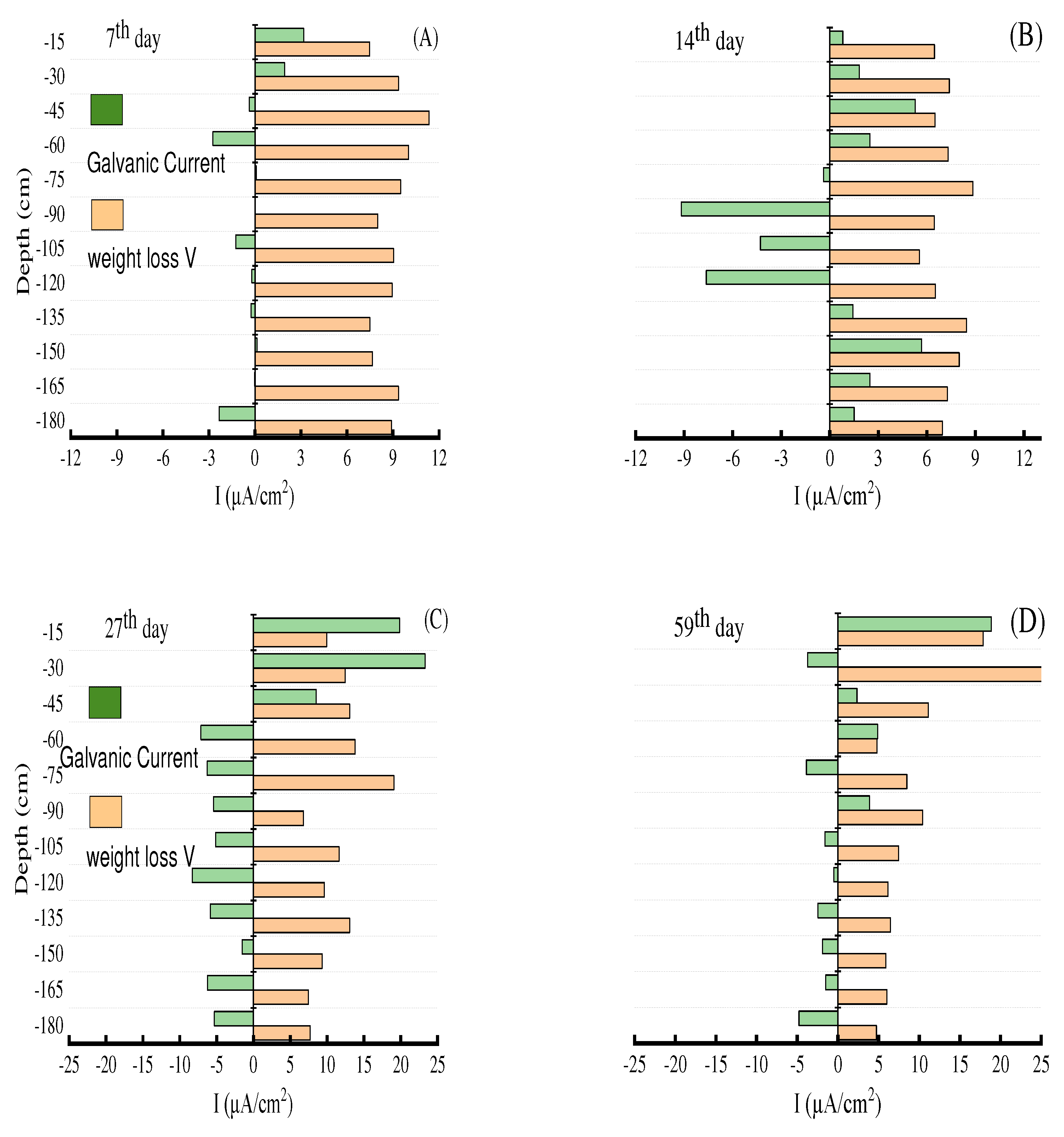

Table 1.
Chemical composition of E690 steel, wt.%.
| C | Si | Mn | P | S | Cr | Ni | Cu | Mo | V | Als | Fe |
| 0.15 | 0.20 | 1.00 | 0.0058 | 0.0014 | 0.99 | 1.45 | 0.0091 | 0.37 | 0.03 | 0.036 | Bal. |
Table 2.
Macrocorrosion morphology of rusted E690 specimens in the simulated thermocline.
| Depth (cm) |
Time | ||||
|---|---|---|---|---|---|
| 7th day | 20th day | 27th day | 44th day | 59th day | |
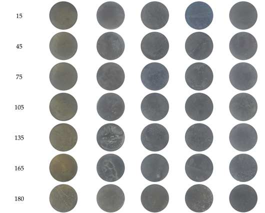 | |||||
Table 3.
Microcorrosion morphology of rusted E690 specimens in the simulated thermocline(100X).
| Depth (cm) |
Time | ||||
|---|---|---|---|---|---|
| 7th day | 20th day | 27th day | 44th day | 59th day | |
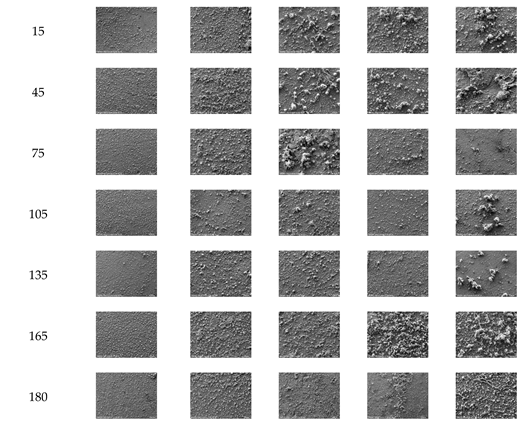 | |||||
Table 4.
Microcorrosion morphology of derusted E690 specimens in the simulated thermocline (200X).
| Depth (cm) |
Time | ||||
|---|---|---|---|---|---|
| 7th day | 20th day | 27th day | 44th day | 59th day | |
 | |||||
Disclaimer/Publisher’s Note: The statements, opinions and data contained in all publications are solely those of the individual author(s) and contributor(s) and not of MDPI and/or the editor(s). MDPI and/or the editor(s) disclaim responsibility for any injury to people or property resulting from any ideas, methods, instructions or products referred to in the content. |
© 2024 by the authors. Licensee MDPI, Basel, Switzerland. This article is an open access article distributed under the terms and conditions of the Creative Commons Attribution (CC BY) license (http://creativecommons.org/licenses/by/4.0/).
Copyright: This open access article is published under a Creative Commons CC BY 4.0 license, which permit the free download, distribution, and reuse, provided that the author and preprint are cited in any reuse.


