Submitted:
23 January 2024
Posted:
24 January 2024
You are already at the latest version
Abstract
Corrugated board, widely used in the packing industry, is a recyclable and durable material. Its strength and cushioning, influenced by geometry, environmental conditions like humidity and temperature, and paper quality, make it versatile. Double-walled (or five-ply) corrugated board, comprising two flutes and three liners, enhances these properties. This study introduces a novel approach to analyze 5-layered corrugated board, extending a previously published algorithm for single-walled boards. Our method focuses on measuring layer and overall board thickness, flute height, and center lines of each layer. Integrating image processing and genetic algorithms, the research successfully developed an algorithm for precise geometric feature identification of double-walled boards. Images were recorded using a special device with a sophisticated camera and image sensor for detailed corrugated board cross-sections. Demonstrating high accuracy, the method faced limitations only with very deformed or damaged samples. This research contributes significantly to quality control in the packaging industry and paves the way for further automated material analysis using advanced machine learning and image sensors. It emphasizes the importance of sample quality and suggests areas for algorithm refinement to enhance robustness and accuracy.
Keywords:
corrugated board
; double-walled
; flute parameters
; cross-section image
; genetic algorithm
1. Introduction
Corrugated board as a material commonly used in the packaging industry has many advantages in comparison to the other packing materials. One can notice its strength, lightweight, ease of customization, recyclable, and relatively low costs. It can effectively protect goods during their shipping, storage and handling.
In single-walled corrugated boards, its structure consists of one flute and two liners. The latter are often manufactured from kraft paper, a kind of paper that comes from wood pulp. It is known from its durability, strength and resistance to puncturing or tearing. These properties make it an ideal material for packaging applications, in particular for the outer layers like liners. The strength, cushioning or smooth surface of the corrugated board are related to the geometry of the internal layer, that is the flute, including its height. The formation of the fluted sheet in the corrugated board involves the paper being fed through a sequence of fluting rollers, resulting in the distinctive ridges and valleys. The higher flutes provide enhanced strength and cushioning, while the smaller flutes are more suitable for printing purpose due to the smoother surface of the resulting corrugated board. The most common flute types are:
- A-flute: its approximated height is 5 mm. A-flute is commonly used for heavy goods packaging, i.e., furniture, due to its strength and cushioning properties.
- B-flute: its approximated height is 3 mm. B-flute has quite universal properties. It is very often used for retail packing or shipping boxes.
- C-flute: its approximated height is 4 mm. It is the most commonly used type of flute and has similar applications to B-flute.
- E-flute: its approximated height is 1.6 mm. It offers a smooth surface, which is appropriate for printing purposes. This type of flute is commonly used for retail packaging and small boxes.
- F-flute: its approximated height is 0.8 mm. It can be applied, similarly to E-flute, for small boxes and retail packing providing good printing properties due to smooth surface of the corrugated board.
The choice of flute type depends on its final specific application. However, it is possible to improve the corrugated board properties by applying the double-walled structure, e.g., to combine cushioning and printing quality or to increase their strength properties. Every kind of flute has particular advantages and is appropriate for certain packing purposes. Manufacturers have the ability to incorporate several flutes in order to produce customized corrugated boards that satisfy certain criteria for strength, cushioning, and printing properties. Double walls available on the market are often composed of BC (5–7 mm), EB (3.5–5 mm), or EC (4–5.5 mm) flutes. Figure 1 presents these examples of flutes combinations in the double-walled corrugated board.
The corrugated board is susceptible to warping both during manufacture and subsequent stages, such as storage, transit, and usage, which may lead to deformation. The origins of these phenomena are attributed to fluctuations in temperature and humidity, as well as mechanical stress. There are two sorts of defects in the corrugated board: global imperfections and local imperfections. Beck and Ficherauer developed and explained a model that accounts for the organized, extensive bending of the cardboard [3]. The writers of this paper mainly focused on local issues. In 1995, Nordstrand conducted a study to investigate how the magnitude of imperfections affects the compressive strength of boxes produced from the corrugated board [4]. In 2004, the author studied local flaws by examining the nonlinear buckling of Rhodes and Harvey orthotropic plates [5]. Lu et al. [6] analyzed the mechanical characteristics of corrugated cardboards, explicitly focusing on the effects of imperfections during compression. Garbowski and Knitter-Piątkowska [7] conducted a detailed analysis of the bending properties of double-walled corrugated cardboard. Mrówczyński et al. [8] suggested a technique to analyze single-walled corrugated cardboard by including original flaws. Cillie and Coetzee conducted a study on corrugated cardboards that had both global and local defects and subjected them to in-plane compression [9]. In a recent study, Mrówczyński and Garbowski introduced a straightforward approach to compute the effective stiffness of the corrugated board with geometric imperfections. This technique utilizes the finite element method and representative volumetric element [10].
Image processing is rarely employed in the study of corrugated boards. Nevertheless, the most prevalent instance is to the development of an automated garbage sorting system. Liu et al. created a novel trash classification model using transfer learning and model fusion [11]. Rahman et al. devised a system for categorizing recyclable waste paper based on template matching [12]. A further use of the image processing approach involves calculating the number of layers in the corrugated board. Cebeci used conventional image processing techniques to automate the numbering of the corrugated board [13]. In a similar manner, Suppitaksakul and Rattakorn used a machine vision system and image processing methods to quantify the number of corrugated boards accurately [14]. Subsequently, Suppitaksakul and Suwannakit proposed an algorithm for merging corrugated board pictures [15].
Classification of various materials and cross-section geometrical features evaluation based on images can be found in the literature. Caputo et al. used the support vector machine algorithm to categorize items by analyzing their photos under different lighting and positioning scenarios [16]. Iqbal Hussain et al. used a convolutional neural network, namely the ResNet-50 architecture, to identify and categorize woven materials [17]. Wyder and Lipson investigated the use of convolutional neural networks to identify the static and dynamic characteristics of cantilever beams using their unprocessed cross-section pictures [18]. Li et al. used a range of deep learning methods to examine the geometric characteristics of a self-piercing riveting cross-section [19]. The authors demonstrated that the SOLOv2 and U-Net topologies provide the most optimal outcomes. Ma et al. examined the geometric characteristics of crushed cross-sections of thin-walled tubes made of carbon fiber-reinforced polymer [20].
The genetic algorithm is an optimization method that takes inspiration from the natural processes of selection and genetics [21]. These algorithms use the concepts of evolution, including selection, crossover, and mutation. The fundamental concept behind genetic algorithms is to generate a group of individuals that reflect potential solutions to a considering issue. Each individual is represented by a collection of characteristics, referred to as chromosomes or genomes, that may be seen as the genetic material. These chromosomes undergo operations such as selection, crossover, and mutation, which mimic the genetic processes of reproduction and variation. John Henry Holland [22] is renowned as the founding figure in the field of genetic algorithms, which have shown remarkable effectiveness across various domains including optimization, scheduling, and artificial intelligence. These algorithms are particularly adept at navigating complex, multidimensional search spaces where conventional optimization methods might struggle. In the realm of corrugated boards, genetic algorithms have found unique applications. Shoukat combined these algorithms with mixed integer linear programming to optimize cost and greenhouse gas emissions in papermaking [23], while Hidetaka and Masakazu utilized them for scheduling in corrugated board production [24].
This paper introduces a novel approach to ascertain the geometric features of corrugated board using a specialized acquisition device and an algorithm combining image processing with genetic algorithms, focusing on flute geometry. This methodology could lay the groundwork for automatically modeling corrugated board geometry from cross-sectional images. This research stands as a important contribution to the field, offering practical and innovative solutions for the packaging industry. By harnessing the power of genetic algorithms for geometric analysis, it opens new avenues for efficient and accurate corrugated board production, potentially revolutionizing current practices and sustainability in the corrugated packaging sector.2. Materials and Methods
2.1. Corrugated Board Cross-Section Images Acquisition
The images of the corrugated board cross-section have been acquired using the device engineered specifically for this purpose. Its precise description can be found in [25]. Images depicting sample cross-sections were taken under uniform conditions, i.e., with controlled LED-sourced illumination and a camera axis perpendicular to the plane of the sample face. Figure 2a presents a 3D model of the device, whereas Figure 2b shows the mutual position of the camera and analyzed corrugated board sample. In the case of double-walled cardboard, placing the sample in the device holder is necessary to ensure that the higher flute is above the finer one. In the following study, as presented in Figure 2c, the flute located above is referred to as , and the one below is .
The device utilizes ArduCam B0197 camera with Sony IMX179 (1/3.2”) image sensor with a resolution of 8 MPx. Acquired images were saved in JPEG format at a maximum resolution of 3264 × 2448 pixels.
2.2. Algorithm for Corrugated Board Geometrical Feature Identification
Figure 3 presents the flow diagram of the proposed algorithm. RGB image obtained from the device is first subjected to different preprocessing operations. Various versions of the input image are then utilized in order to identify several geometrical features of a 5-layer corrugated board sample, such as its height, flutes’ heights, periods and phase shifts, liners’ and flutes’ thickness. The algorithm has been implemented in Python using the OpenCV and geneticalgorithm libraries.
2.2.1. Image Preprocessing
The input of the system was a single frame from the camera. It was an RGB image with dimensions of 3264 × 2448 pixels. The first preprocessing operation is a grayscale conversion into range <0,255>. Next, an 800 × 800 pixels subset of a grayscale image is cut out of the central acquisition area. Figure 4a presents the final image acquired as a result of described actions. In order to remove small noise from the image (caused by the presence of cellulose fibers), two blurring methods were applied: averaging with a normalized box filter and with a kernel size of 3 × 3 and bilateral filter. Figure 4b presents the result of these operations. Finally, the blurred image was converted into a binary image (Figure 4c) by applying lower threshold binarization with a threshold value equal to 75. All the parameters in the preprocessing stage were chosen empirically.
2.2.2. Corrugated Cardboard Thickness Estimation
The thickness of 5-layer corrugated cardboard can be estimated with the same method used for 3-layer samples that was presented in [25]. The boundary points of outer liners can be identified by applying column-wise scanning of the binary image (Figure 4c). Pixels in each column of the image are analyzed. The y coordinate of the first white pixels in each column is saved to ULEP matrix for scanning from the top of the image towards the bottom. Next, scanning is continued until the first black pixel is recognized. Its y coordinate is written to ULIP matrix. As a result, external points of the upper liner are written in the ULEP matrix, whereas ULIP contains upper liner internal points. Analogically, in order to determine lower liner boundary points, the direction of column-wise scanning is reversed, starting from the bottom of the image towards the top. In that way, new matrices LLEP and LLIP, which respectively store external and internal pixels of the lower liner, are created. Figure 5 presents the result of this operation.
In order to determine the corrugated board sample height , the average distance between external points of the upper and lower liner are calculated. It can be expressed as
where denotes the column index, and is the total number of columns.
For the purpose of further geometrical features identification, the external boundaries of both upper and lower liners are approximated using linear functions and coordinates from ULEP and LLEP matrixes. The resulting linear equations can be expressed as
where and denote the parameters of the upper liner approximation, while and are the parameters of the lower liner approximation.
2.2.3. Flutes Center Lines and Heights Estimations
At this stage, the corrugated cardboard flutes center lines and heights are estimated. The binary image row sum curve is plotted to find the localization of liners and flutings regions. Analyzing the number of white pixels in each row of the image, as presented in [25], allows us to determine the approximate location in the image of the bottom and upper liner. The sample is placed horizontally, and curve local maximums are related to the presence of flat layers. Therefore, the occurrence of an additional liner in the middle of the sample should create one additional extremum visible on the curve. In the case of the 5-layered corrugated board sample, which consists of 3 liners and 2 flutes, 3 local maximums should always be detected at this stage. In order to smooth the row sum curve and highlight the maximum resulting from liners, the same version of the Savitzky–Golay filter with 30 interpolation points and a first-degree polynomial was applied. Furthermore, the distance between maximums has to be larger or equal to 20, and the minimal value of the local maximum was equal to 0.4 of the global maximum value. Figure 6a depicts the original row sum and smoothed curves with 3 local maximums detected. It is also worth noting that the peak values can differ significantly for both the ideal and the creased samples. Their values mainly depend on the overall arrangement of layers and their thickness.
At this point, the row sum curve can be further analyzed. Based on local maximums, the curve is divided into 3 ranges. Each range corresponds to the area of one liner. Ranges borders (black bold dashed line) are determined as middle points between two adjacent local maximums marked as blue bold dots in Figure 6a. In Figure 6b, the bottom, middle, and upper liner ranges are marked in green, blue, and red, respectively. In each of these intervals, the subsequent actions are carried out:
- The local maximum is identified.
- The vertical line with an ordinate equal to the value of 0.9 (for bottom and upper liner regions, or 0.9 for middle liner region) is now plotted. Two intersection points of the curve and plotted line are determined and marked by bold dots visible in Figure 6b.
- The distance between intersection points within each range is calculated and denoted as , and for the upper, middle, and bottom liners, respectively.
For the 5-layer corrugated board samples, the center line and height estimations are calculated separately for each fluting. First, the middle liner approximate location in the image must be determined. Another column-wise scanning of the binary image (Figure 4c) is carried out. Scanning is limited to the rows with coordinates , where and are consecutive intersection points of the middle liner visible in Figure 6b. The coordinates of the first white pixels in each column are written into the MLUP matrix for scanning from the top to the bottom of the image and for reversed direction into MLBP. A linear approximation of a line passing through the center of the area bounded by MLUP and MLBP pixels is performed. It can be expressed as:
where and denote the parameters of the middle liner approximation. Figure 7 shows results of above operations.
Both flutings searching can be now limited based on the boundaries of the liners expressed in Equations (2), (3), and (4). The boundary lines limiting the searching can be written in the following forms
whereas for limiting the
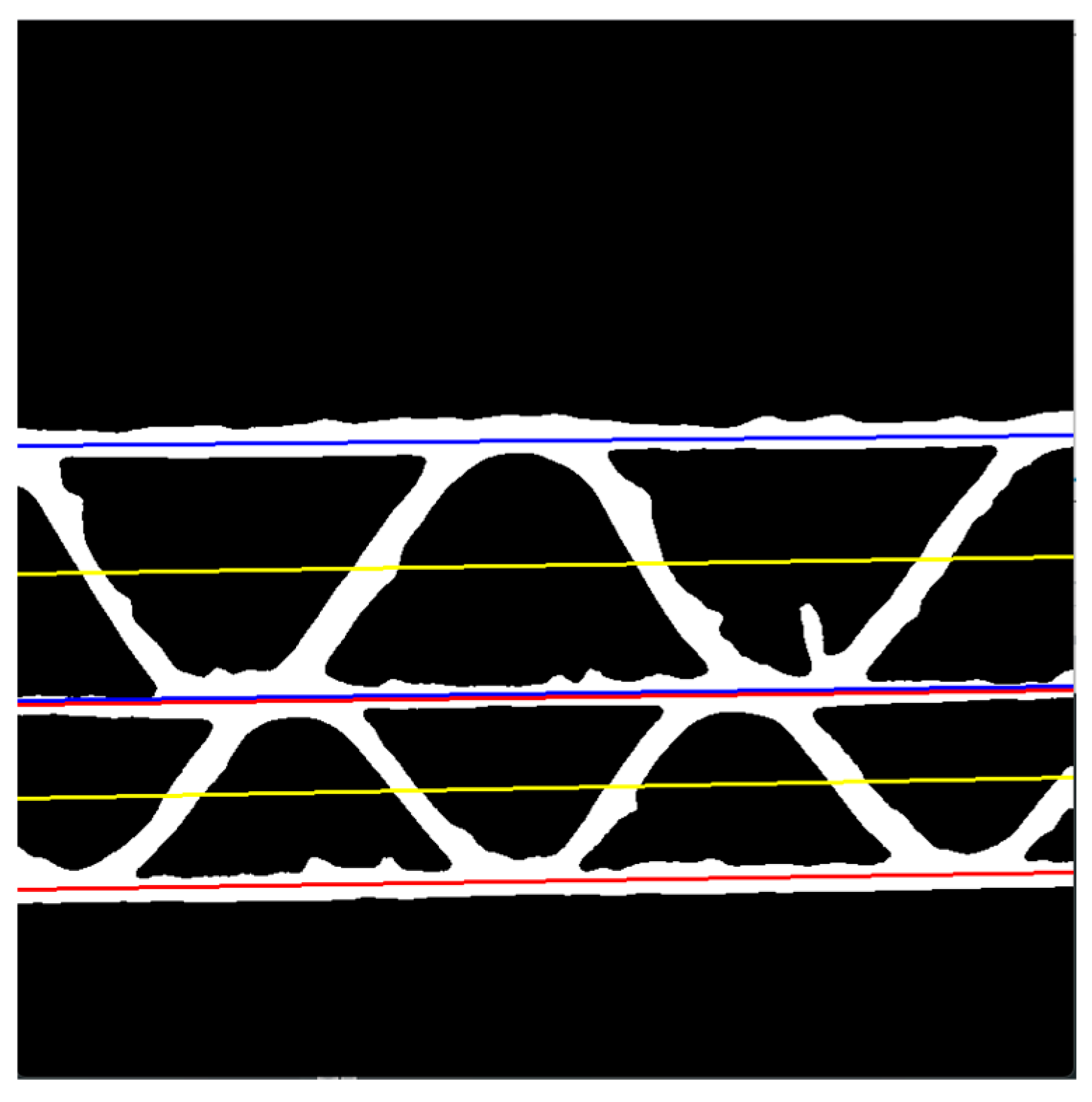
The boundary lines are depicted in Figure 8 in red and blue, while the center lines are presented in yellow. The center lines are approximated as central lines between two boundary lines, for each flute, respectively, and can be expressed as:
where , are the parameters of the center lines.
The heights of the flutes can be approximated using the following formulas
It is worth noting, that flutes height is equal to two times the amplitude of the sinusoidal function.
Figure 8.
The binary image with boundary lines for limiting the searching areas for (blue lines) and (red lines), and the central lines (yellow lines).
Figure 8.
The binary image with boundary lines for limiting the searching areas for (blue lines) and (red lines), and the central lines (yellow lines).
2.2.4. Flute Period Searching Range
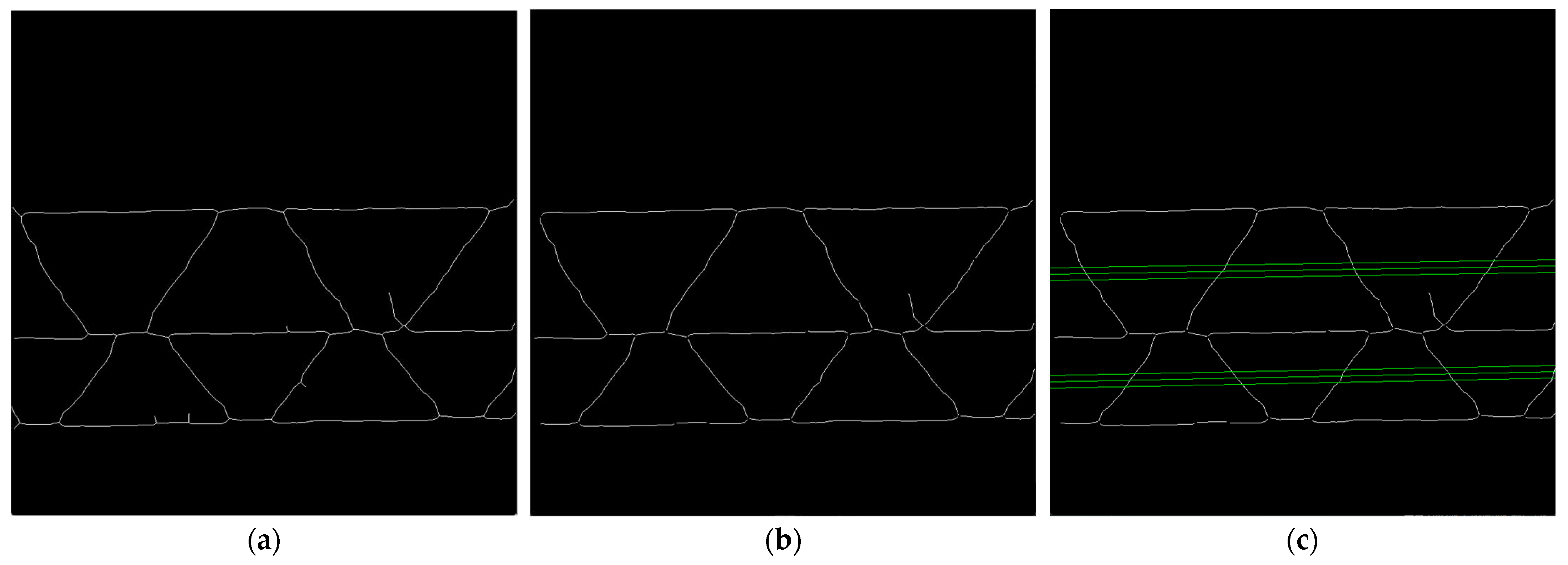
Next, the binary image is skeletonized. The result of this operation is presented in Figure 9a. The presence of protruding fibers in the cross-section of the sample can cause some disturbances in the form of side branches in the skeleton. A custom filtering function is applied to the skeletonized image to filter out the unwanted offshoots. As a result, all side branches with contour lengths less than 50 pixels are removed, see Figure 8b.
The limitation of period searching is necessary for genetic algorithm to provide credible solutions. Values and (the range of the period searching in pixels for -th fluting) are based on calculating the distances between the intersection points of the skeleton contours, with 3 lines parallel to the flutings center line, drawn through the flute area, see Figure 8c. The average distance between successive intersection points and the maximum distance is determined for each fluting. The values , and are taken, where is the average distance between the intersection points for the 3 parallel lines, and denotes the maximal value of the distances between these intersection points for -th fluting. In case of too many disturbances, e.g., due to the presence of long side branches or critical deformation of the sample, the default values , are set.
Figure 8.
(a) Results of the skeletonization process; (b) results after skeletonization process and removing side branches; (c) three parallel green lines for each fluting period limitations.
Figure 8.
(a) Results of the skeletonization process; (b) results after skeletonization process and removing side branches; (c) three parallel green lines for each fluting period limitations.
2.2.5. Application of the Genetic Algorithm for Flutes Parameters Approximation
Genetic algorithm implemented in [25] enabled the authors to determine sinusoidal function parameters, such as period and phase shift, to asses fluting layer geometrical features. In the case of double-wall corrugated board samples, the genetic algorithm ought to be used for each flute independently.
In the searching process for the parameters of flutes, the following formulas for its approximation were taken into account:
where the parameters , , and amplitude are fluting parameters determined in the previous stages of the proposed algorithm. The solution from the genetic algorithm is a set of two values: phase shift and the period , where i denotes the fluting index (). Two separate genetic algorithm runs provided an independent set of parameters for each fluting.
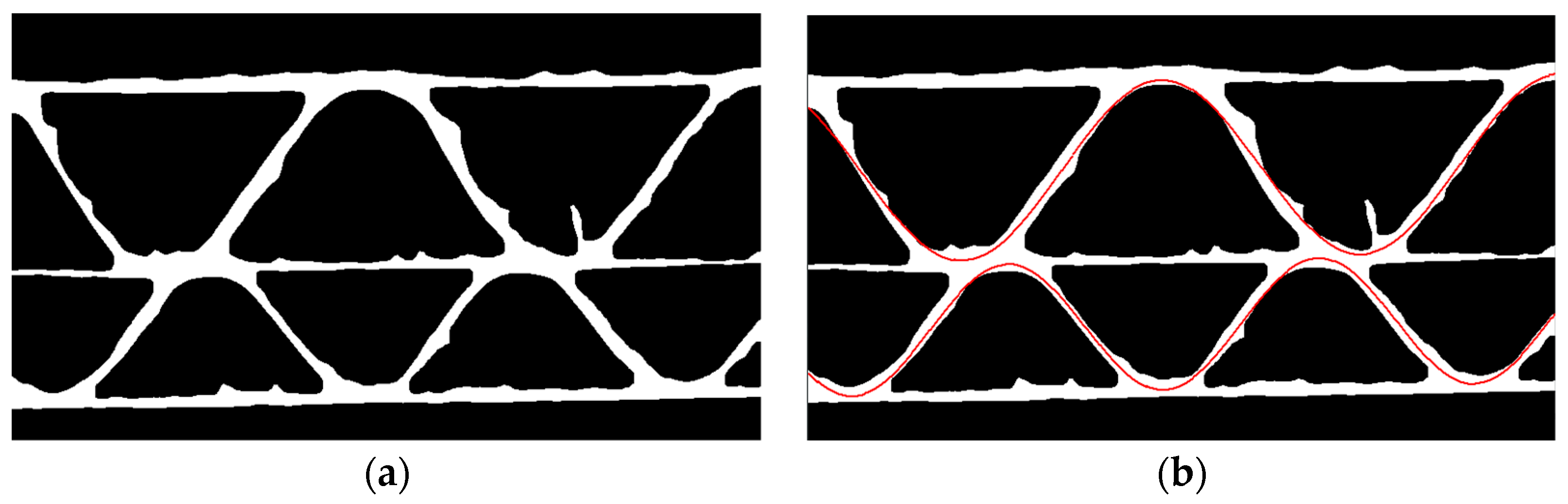
In each run, the genetic algorithm takes the eroded version of the binary image as an input, as shown in Figure 9a. The main reason for utilizing erosion is to narrow down the flute region, so that the sine function approximation is more precise. The phase shift and period search is limited by , , , and , where i denotes the fluting index. The objective function is defined as a total sum of the common pixels for the eroded image and function expressed in Equation (7) or (8) (depending on the analyzed flute) for the given and .
Applying the genetic algorithm, the following parameters were utilized:
- Maximal number of iterations: 500;
- Population size: 100;
- Mutation probability: 0.15;
- Elite group ratio: 0.01;
- Crossover probability: 0.2;
- Parents portion: 0.2;
- Crossover type: uniform.
An example of the genetic algorithm result is presented in Figure 9b.
Figure 9.
(a) The eroded image; (b) an example of the result obtained after the optimization processes using the genetic algorithm (red lines).
Figure 9.
(a) The eroded image; (b) an example of the result obtained after the optimization processes using the genetic algorithm (red lines).
2.2.6. Estimation of the Corrugated Cardboard Layers Thicknesses
Figure 10 depicts a graphic representation of the idea for measuring the thickness of paper layers. The approximate location of flutes in the image is determined based on the sinusoidal function approximations performed in the previous stages of the algorithm. It provides enough information to choose the regions for layers thickness measurement. Areas around layer bonding points are more distorted and have usually higher number of disturbances such as protruding fibers. The area of the upper liner, where the thickness can be measured, is marked in blue. A similar region for the middle and bottom liner is marked in orange and turquoise, respectively. The pink and green colors indicate the areas in which the thickness of the flutings is determined. Figure 11 shows an example of the result.
3. Results
The proposed method allowed the authors to identify the geometrical parameters of any double-wall corrugated board sample in a fully automatic manner. Unfortunately, damaging the structure of layers or severe cross-section crushing may cause unreliable and false results.
Figure 12 presents the results for exemplary corrugated boards samples with BC, EB, EC, and EE flutes. The results in the form of identified geometrical features in pixels and millimeters are summarized in Table 1.
The developed algorithm has limitations similar to those for single-wall samples presented in [25]. It has to do with the fact that the quality of the sample is the most important factor in terms of the credibility of the obtained results. Every imperfection in the form of, e.g., protruding fibers or corrugated layer deformation resulting from crushing can affect the precision of the method. All samples were cut on an oscillating knife-cutting machine, which creates irregular cut edges and visible shreds of cellulose fibers in all specimens.
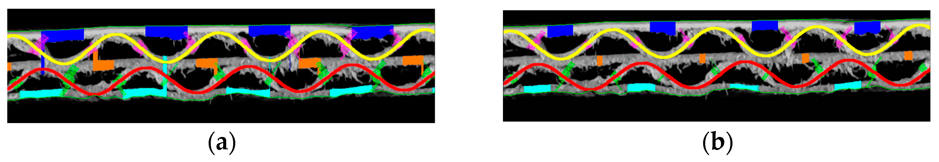
In Figure 13, two BC flute samples are presented. The one on the left is not damaged in any way by creasing. The sample on the right is crushed stochastically with a visible change in fluting shape. It can be noticed that the algorithm still solves the sinusoidal function approximation, but it does not reflect the deformed corrugated layer shape. In that case, the flute period and height are not correctly measured but can be used to estimate the actual flute type of the crushed sample. Table 2 contains the identified parameters for these two samples.
Figure 14 shows two samples of the corrugated board with flute EB and the results of their geometrical features identification. The corrugated board on the left is without any damage and the one on the right – with damage in the form of a crushed flute and multiple protruding cellulose fibers. The identified geometrical parameters for both samples with flute EB are presented in Table 3.
Examples presented in Figure 15 depict two EC flute specimens cut out from the same cardboard sheet. The one on the left is a reference sample, whereas on the right is the sample with the cutting edge, which was crushed by creasing. The results of processing both images are visible in Table 4. Severe deformation of the higher fluting is again causing a low-precision sine approximation. Period and height measurements in the case of lower flutes are more reliable since creasing is less visible in the cross-section. On the other hand, in the case of E flutes, the presence of noise in the form of jagged edges and cellulose fibers intensifies because of the reduced distance between each layer. Hence, difficulties with obtaining reliable layer thickness measurements can occur.
The last example is shown in Figure 16, where two samples of corrugated board with EE flute are presented. Since the sample combines two of the lowest possible flutes of all the cases presented here, it is supposedly the most difficult to analyze. The crease in such cardboard is less visible (example on the right). Nevertheless, as the geometrical dimensions of the cross-section are reduced, the most significant trouble is measuring the thickness of individual paper layers. As can be noticed in the exemplary results in Figure 16b, the measured liners and flute areas are not marked correctly; hence, the measurements are flawed. This complex problem is further elaborated on in the discussion section. Table 5 presents the results of the parameters identification for both samples of corrugated board with EE flute.
The presented results are only a small part of the sample images processed during this research. A total number of 310 different images were processed with the proposed algorithm. The database consisted of reference, stochastically deformed (different forces applied at different locations), and crushed by creasing corrugated board samples.
4. Discussion
In the results section, some exemplary outcomes from the algorithm for various cardboard samples were presented. In order to evaluate this, in some way innovative, method for identifying cross-section corrugated board geometrical features, the following section takes up the critical discussion of the results and the limitations of the proposed approach.
As previously emphasized, the method’s effectiveness relies significantly on the precision of sample cutting. Cellulose shreds and protruding fibers visible in each cross-section are a side effect of using an oscillating knife as a cutting tool. Since their presence affects the outcome to a great extent, excising the samples by using, e.g., a laser cutter, is expected to provide more trustworthy results. Another important factor that affected the accuracy of the algorithm was damages introduced into the corrugated board in the process of stochastic deformation and creasing.
As described in [25], delamination of layers, corrugated layer crushing, and the presence of jagged edges create noticeable difficulties in determining the thickness of each paper layer. These difficulties can also be found in the presented examples, e.g., in Figure 16d (visibly flawed liners thickness measurement caused by cellulose fibers) and Figure 15d (flawed flutes thickness measurement caused by its high level of crush). The most reliable geometric parameters obtained from the algorithm seem always to be the period of the corrugated layer. Even in cases of inaccurate fit of the approximating function, which was assumed as a sine function, to the shape of visibly crushed fluting, the period measurement can be considered a reasonable approximation (Figure 13d and Figure 15d). In those scenarios, the heights of corrugated layers are not entirely credible and can be considered as auxiliary indicators.
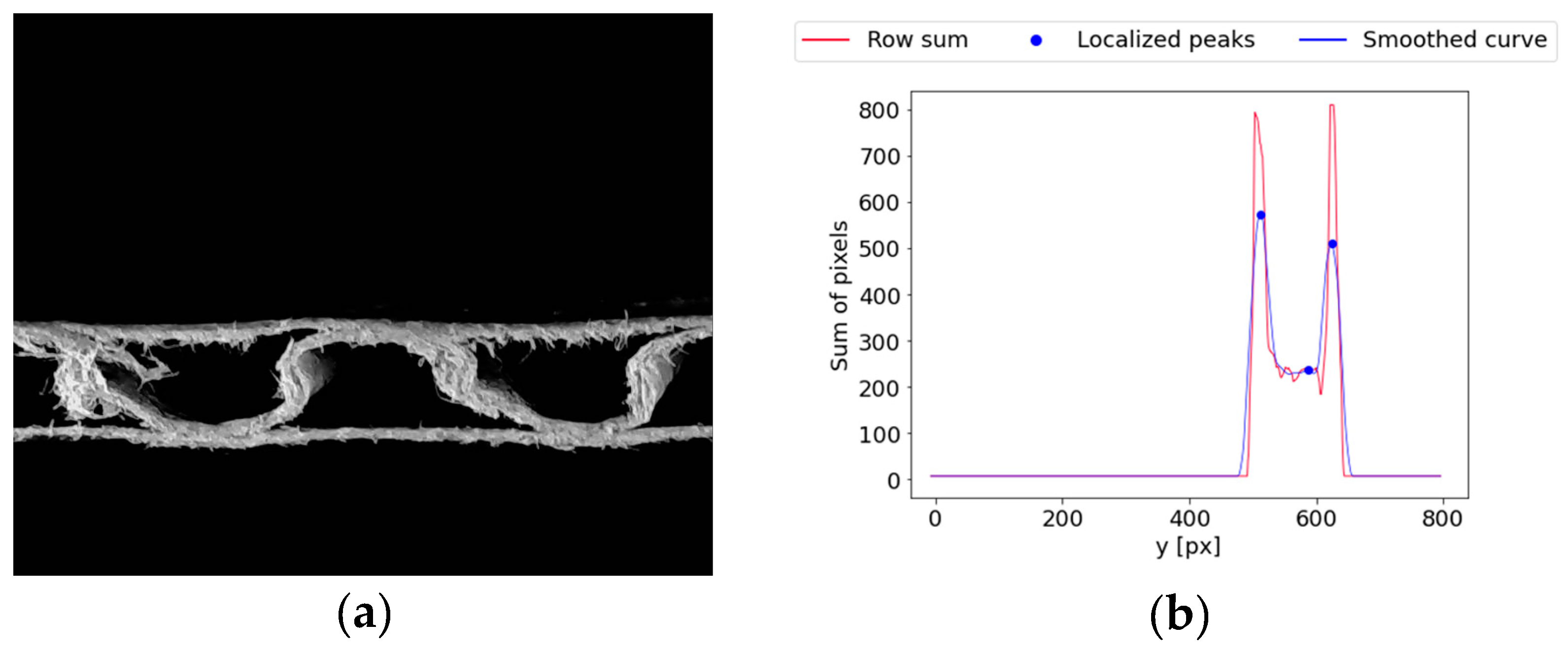
Another problem can occur during the analysis of the cross-section of different samples. Figure 17a shows a single-wall C-flute sample with a visible hank of cellulose fibers on the left side of the image in the region between liners. Figure 17b depicts a smoothed row sum curve with detected peaks for this sample. Three local maximums were recognized in the first stages of the algorithm. Usually, that would indicate a double-wall cardboard type, which, in this case, is obviously incorrect. The workflow of the algorithm differs significantly for single and double-wall corrugated board samples. Therefore, the obtained results would be unfit for further use.
Figure 17.
Example of the error in recognizing the number of layers in the corrugated board sample: (a) a single-wall C-flute sample with a visible hank of cellulose fibers; (b) a smoothed row-sum curve of the image with wrongly localized peaks potentially reflecting the liners of the corrugated board.
Difficulty in measurements of the liner thickness can also be caused by factors other than cross-section noise. Figure 18 depicts a relatively common (among samples processed in the research) case of both flutes being in phase with each other, meaning the phase shifts for both corrugated layers are almost identical. Considering that the regions for measuring each layer thickness are calculated based on the approach presented in Figure 10, it is impossible for the algorithm to obtain a credible area for middle liner thickness measurement. This results in the method providing an incomplete set of geometrical features of the sample.
The biggest issue with the proposed method is commonly visible in processing microwave samples. The layers thickness measurement was flawed in most of the processed flute EE corrugated board images. It is due to too much interference (jagged fibers) concerning the size of the area between layers. A possible solution to this problem may be to limit the regions for measuring thickness for each layer. Different conditions for microwave flutes adopted in the approach presented in Figure 10 can improve the efficiency of the algorithm. Figures 19a and 19b present results for the same image before and after limiting the areas, respectively. The improved approach provides significantly better results. Nonetheless, some errors, especially in fluting thickness measurement, still occur.
Figure 17.
(a) The original example (very weak effect) and (b) the results on the same image after limiting the layers thickness measurement areas.
Figure 17.
(a) The original example (very weak effect) and (b) the results on the same image after limiting the layers thickness measurement areas.
5. Conclusions
In this paper, the method for identifying geometric features of double-wall corrugated board cross-sections is presented. The cross-section images were collected using the device first introduced in [Rogalka2023], where a similar algorithm was successfully applied for single-wall corrugated cardboard. This enhanced method primarily yield reliable results for 5-ply samples, widely used in the packaging industry. Geometrical characteristics of the sample were determined through complex image processing techniques and genetic algorithms. The use of local algorithms, such as gradient-base ones, is not feasible to the specific nature of the optimization problem.
The methods effectiveness and reliability largely depend on the quality of the sample. The fit of the approximation function to the flute’s shape, in terms of height and period, is strongly affected by the extent of the cardboard’s cross-section crushing. Additionally, cutting corrugated boards on an oscillating knife-cutting machine, a common industry practice, aligns well with this method, enabling its practical applications.
In summary, while the method has some limitations, improvements seem feasible in the near future. A quick and relatively simple algorithm for extracting geometrical features could be a crucial step in automating the modeling of corrugated board structure.
Author Contributions
Conceptualization, T.G. and M.R.; methodology, M.R. and J.K.G.; software, M.R.; validation, M.R., J.K.G. and T.G.; formal analysis, M.R.; investigation, M.R. and J.K.G.; resources, M.R. and T.G.; data curation, M.R.; writing—original draft preparation, M.R., J.K.G. and T.G.; writing—review and editing, J.K.G. and T.G.; visualization, M.R.; supervision, J.K.G.; project administration, J.K.G. and T.G.; funding acquisition, J.K.G. and T.G. All authors have read and agreed to the published version of the manuscript.
Funding
This research received no external funding.
Institutional Review Board Statement
Not applicable.
Informed Consent Statement
Not applicable.
Data Availability Statement
Data are available on request.
Acknowledgments
The authors would like to thank Kacper Andrzejak from the Werner Kenkel company and Monika Niziałek-Łukawska and Małgorzata Kuca from the Schumacher Packaging company for providing the research materials. We would also like to thank the Femat company for providing financial support for the conducted research and for the possibility of using laboratory equipment as well as professional software.
Conflicts of Interest
The authors declare no conflicts of interest.
References
- Pereira, T.; Neves, A.S.L.; Silva, F.J.G.; Godina, R.; Morgado, L.; Pinto, G.F.L. Production Process Analysis and Improvement of Corrugated Cardboard Industry. Procedia Manuf. 2020, 51, 1395–1402. [Google Scholar] [CrossRef]
- Di Russo, F.M.; Desole, M.M.; Gisario, A.; Barletta, M. Evaluation of wave configurations in corrugated boards by experimental analysis (EA) and finite element modeling (FEM): The role of the micro-wave in packing design. Int. J. Adv. Manuf. Technol. 2023, 126, 4963–4982. [Google Scholar] [CrossRef] [PubMed]
- Beck, M.; Fischerauer, G. Modeling Warp in Corrugated Cardboard Based on Homogenization Techniques for In-Process Measurement Applications. Appl. Sci. 2022, 12, 1684. [Google Scholar] [CrossRef]
- Nordstrand, T.M. Parametric study of the post-buckling strength of structural core sandwich panels. Compos. Struct. 1995, 30, 441–451. [Google Scholar] [CrossRef]
- Nordstrand, T. Analysis and testing of corrugated board panels into the post-buckling regime. Compos. Struct. 2004, 63, 189–199. [Google Scholar] [CrossRef]
- Lu, T.J.; Chen, C.; Zhu, G. Compressive behaviour of corrugated board panels. J. Compos. Mater. 2001, 35, 2098–2126. [Google Scholar] [CrossRef]
- Garbowski, T.; Knitter-Piątkowska, A. Analytical Determination of the Bending Stiffness of a Five-Layer Corrugated Cardboard with Imperfections. Materials 2022, 15, 663. [Google Scholar] [CrossRef] [PubMed]
- Mrówczyński, D.; Knitter-Piątkowska, A.; Garbowski, T. Numerical Homogenization of Single-Walled Corrugated Board with Imperfections. Appl. Sci. 2022, 12, 9632. [Google Scholar] [CrossRef]
- Cillie, J.; Coetzee, C. Experimental and Numerical Investigation of the In-Plane Compression of Corrugated Paperboard Panels. Math. Comput. Appl. 2022, 27, 108. [Google Scholar] [CrossRef]
- Mrówczyński, D.; Garbowski, T. Influence of Imperfections on the Effective Stiffness of Multilayer Corrugated Board. Materials 2023, 16, 1295. [Google Scholar] [CrossRef] [PubMed]
- Liu, W.; Ouyang, H.; Liu, Q.; Cai, S.; Wang, C.; Xie, J.; Hu, W. Image recognition for garbage classification based on transfer learning and model fusion. Math. Probl. Eng. 2022, 2022, 4793555. [Google Scholar] [CrossRef]
- Rahman, M.O.; Hussain, A.; Scavino, E.; Hannan, M.A.; Basri, H. Recyclable waste paper sorting using template matching. In Proceedings of the Visual Informatics: Bridging Research and Practice, First International Visual Informatics Conference, IVIC 2009, Kuala Lumpur, Malaysia, 11–13 November 2009; Zaman, H.B., Robinson, P., Petrou, M., Olivier, P., Schröder, H., Shih, T.K., Eds.; Springer: Berlin/Heidelberg, Germany, 2009; pp. 467–478. [Google Scholar] [CrossRef]
- Cebeci, U.; Aslan, F.; Çelik, M.; Aydın, H. Developing a new counting approach for the corrugated boards and its industrial application by using image processing algorithm. In Practical Applications of Intelligent Systems; Advances in Intelligent Systems and Computing, Wen, Z., Li, T., Eds.; Springer: Berlin/Heidelberg, Germany, 2014; Volume 279, pp. 1021–1040. [Google Scholar] [CrossRef]
- Suppitaksakul, C.; Rattakorn, M. Machine vision system for counting the number of corrugated cardboard. In Proceedings of the International Electrical Engineering Congress (iEECON), Chonburi, Thailand, 19–21 March 2014; pp. 1–4. [Google Scholar] [CrossRef]
- Suppitaksakul, C.; Suwannakit, W. A combination of corrugated cardboard images using image stitching technique. In Proceedings of the 15th International Conference on Electrical Engineering/Electronics, Computer, Telecommunications and Information Technology, Chiang Rai, Thailand, 18–21 July 2018; pp. 262–265. [Google Scholar] [CrossRef]
- Caputo, B.; Hayman, E.; Fritz, M.; Eklundh, J.-O. Classifying materials in the real world. Image Vis. Comput. 2010, 28, 150–163. [Google Scholar] [CrossRef]
- Iqbal Hussain, M.A.; Khan, B.; Wang, Z.; Ding, S. Woven Fabric Pattern Recognition and Classification Based on Deep Convolutional Neural Networks. Electronics 2020, 9, 1048. [Google Scholar] [CrossRef]
- Wyder, P.M.; Lipson, H. Visual design intuition: Predicting dynamic properties of beams from raw cross-section images. J. R. Soc. Interface 2021, 18, 20210571. [Google Scholar] [CrossRef] [PubMed]
- Li, M.; Liu, Z.; Huang, L.; Chen, Q.; Tong, C.; Fang, Y.; Han, W.; Zhu, P. Automatic identification framework of the geometric parameters on self-piercing riveting cross-section using deep learning. J. Manuf. Process. 2022, 83, 427–437. [Google Scholar] [CrossRef]
- Ma, Q.; Rejab, M.R.M.; Azeem, M.; Idris, M.S.; Rani, M.F.; Praveen Kumar, A. Axial and radial crushing behaviour of thin-walled carbon fiber-reinforced polymer tubes fabricated by the real-time winding angle measurement system. Forces Mech. 2023, 10, 100170. [Google Scholar] [CrossRef]
- Goldberg, D.E. Genetic Algorithms in Search, Optimization, and Machine Learning; Addison-Wesley Publishing Company, Inc.: Reading, MA, USA, 1989. [Google Scholar]
- Holland, J.H. Adaptation in Natural and Artificial Systems; University of Michigan Press: Ann Arbor, MI, USA, 1975. [Google Scholar]
- Shoukat, R. Green intermodal transportation and effluent treatment systems: Application of the genetic algorithm and mixed integer linear programming. Process Integr. Optim. Sustain. 2023, 7, 329–341. [Google Scholar] [CrossRef]
- Hidetaka, M.; Masakazu, K. Multiple objective genetic algorithms approach to a cardboard box production scheduling problem. J. Jpn. Ind. Manag. Assoc. 2005, 56, 74–83. [Google Scholar]
- Rogalka, M.; Grabski, J.K.; Garbowski, T. Identification of Geometric Features of the Corrugated Board Using Images and Genetic Algorithm. Sensors 2023, 23, 6242. [Google Scholar] [CrossRef] [PubMed]
Figure 1.
Examples of typical flutes combinations in the double-walled corrugated.
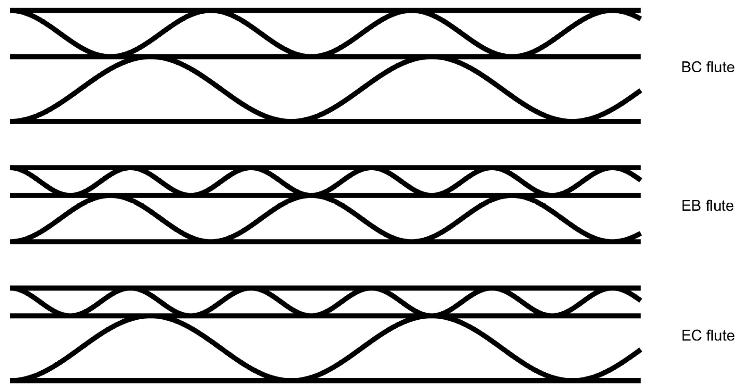
Figure 2.
Device for corrugated board image acquisition: (a) a 3D model of the device; (b) the mutual position of the device components: 1—corrugated board sample; 2—camera; 3—LED strip [Rogalka2023]; (c) fluting indexing.
Figure 2.
Device for corrugated board image acquisition: (a) a 3D model of the device; (b) the mutual position of the device components: 1—corrugated board sample; 2—camera; 3—LED strip [Rogalka2023]; (c) fluting indexing.

Figure 3.
Flow diagram of the proposed method.
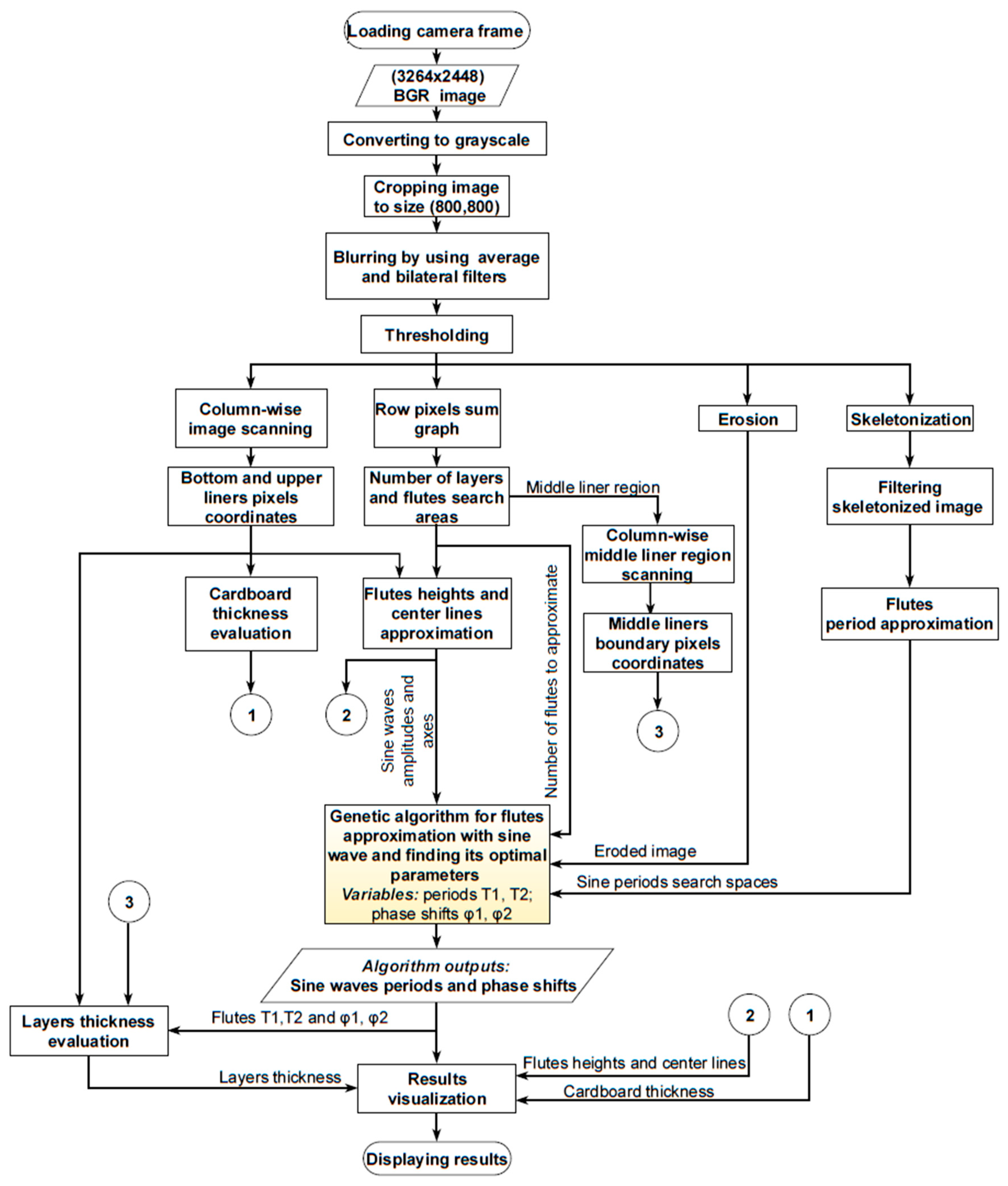
Figure 4.
Images obtained as a result of the preprocessing stage: (a) a grayscale image cropped to 800 × 800 pixels; (b) blurred image; (c) binary image.
Figure 4.
Images obtained as a result of the preprocessing stage: (a) a grayscale image cropped to 800 × 800 pixels; (b) blurred image; (c) binary image.
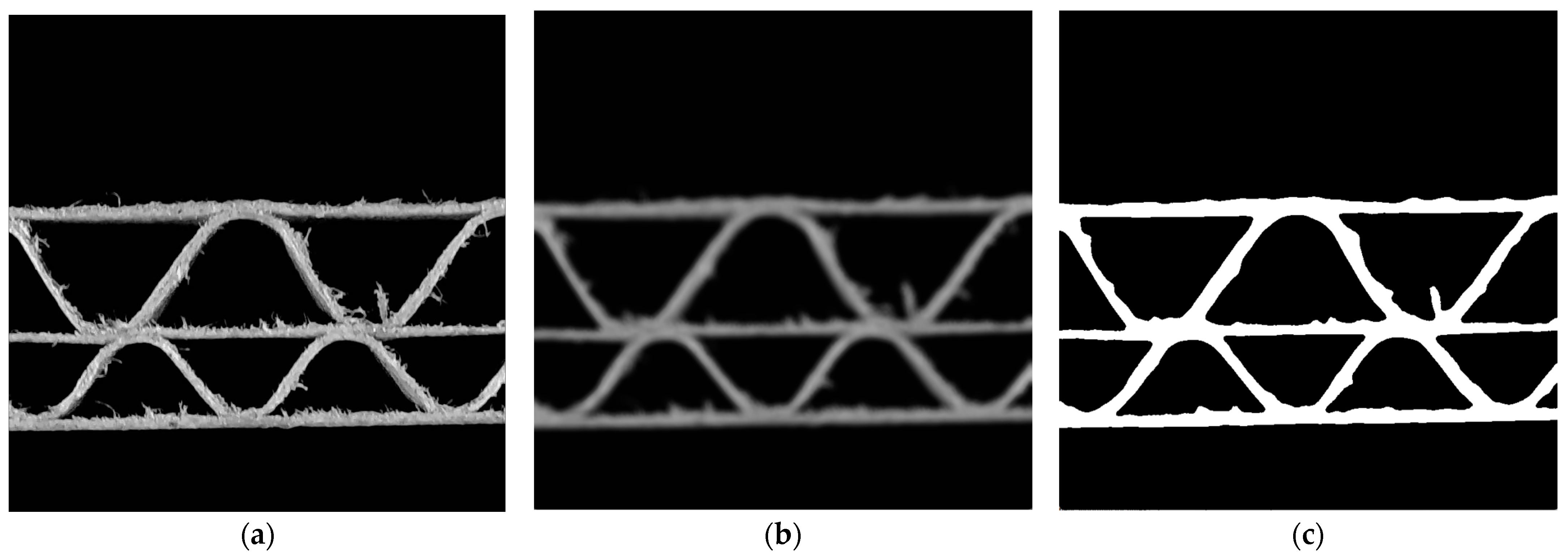
Figure 5.
Internal and external pixels coordinates of the upper and lower liners.
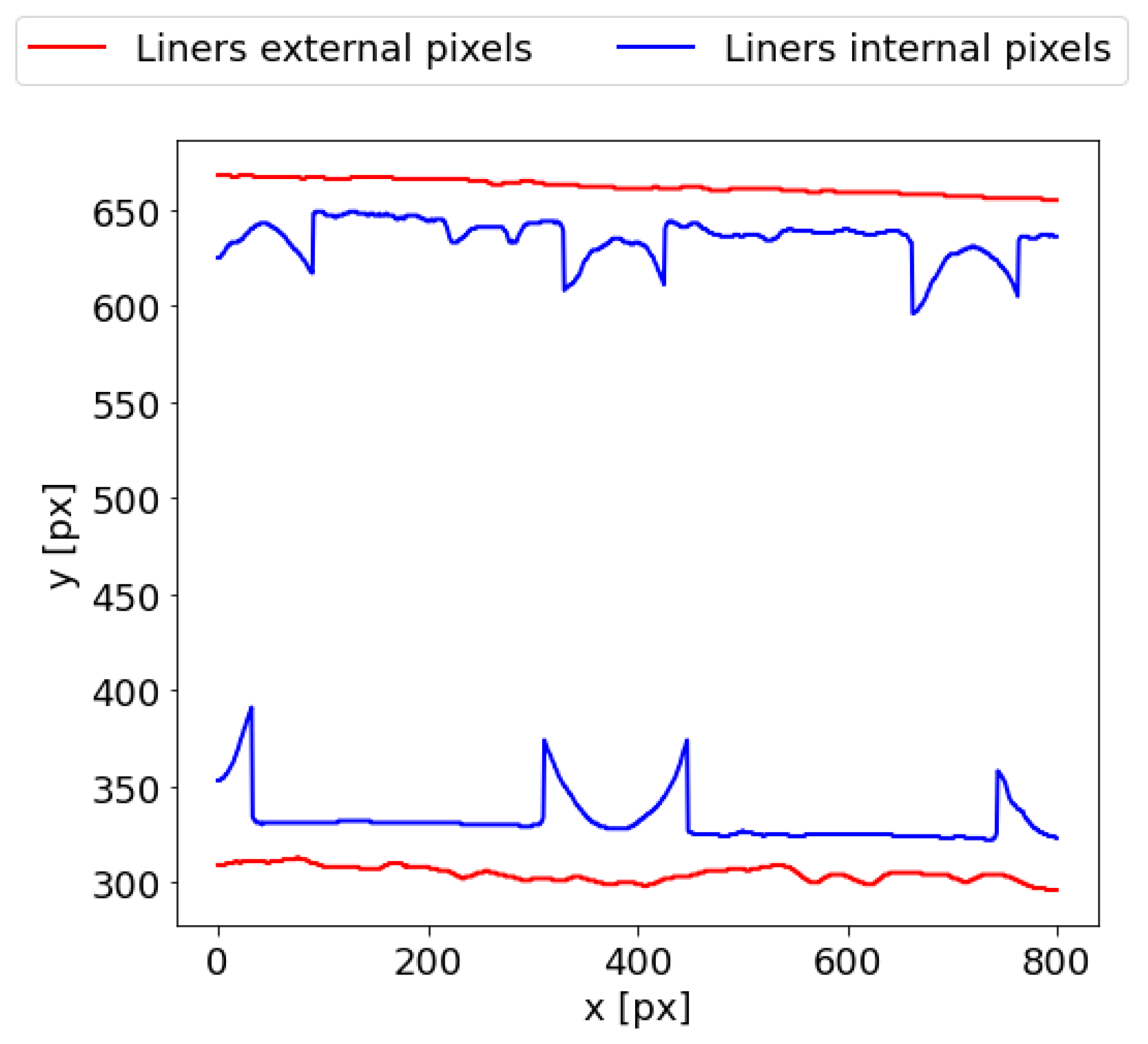
Figure 6.
The row sum curve and localizations of the vertical positions of liners: (a) the row sum curve (red line) and the smoothed curve (blue line); (b) the upper (red), middle (blue) and lower (green) liners’ ranges.
Figure 6.
The row sum curve and localizations of the vertical positions of liners: (a) the row sum curve (red line) and the smoothed curve (blue line); (b) the upper (red), middle (blue) and lower (green) liners’ ranges.
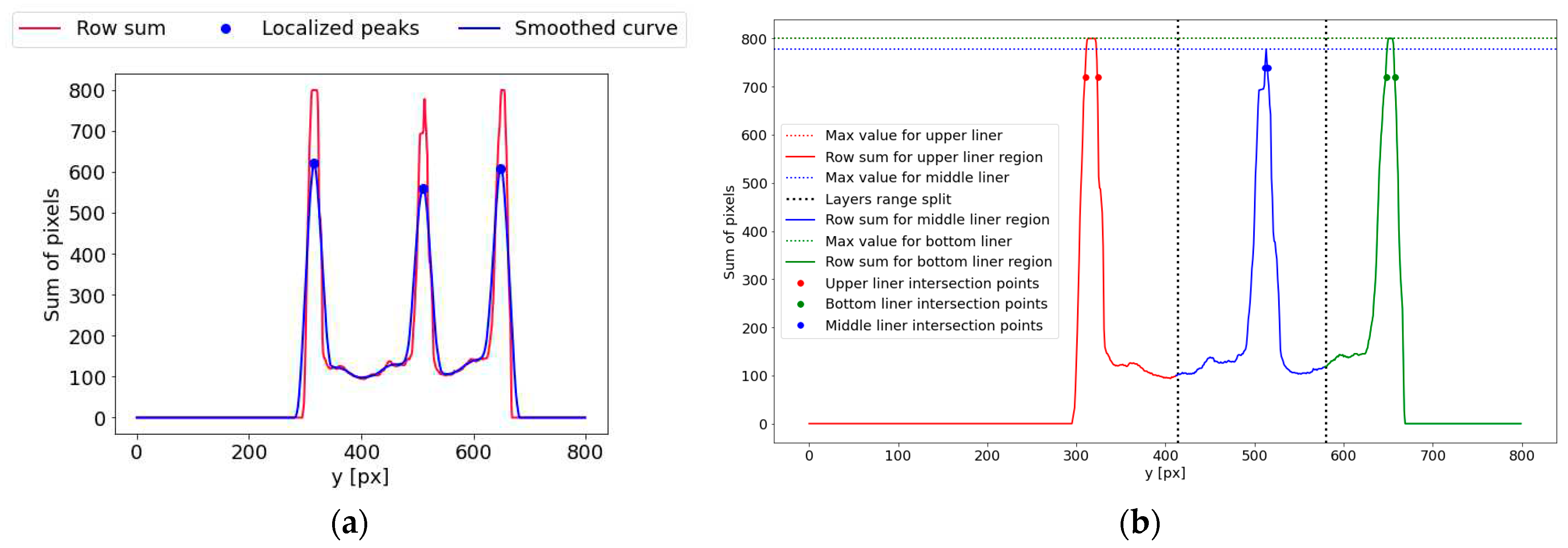
Figure 7.
Binary image with the upper (green) and bottom (orange) pixels of the middle liner and its linear approximation (blue).
Figure 7.
Binary image with the upper (green) and bottom (orange) pixels of the middle liner and its linear approximation (blue).
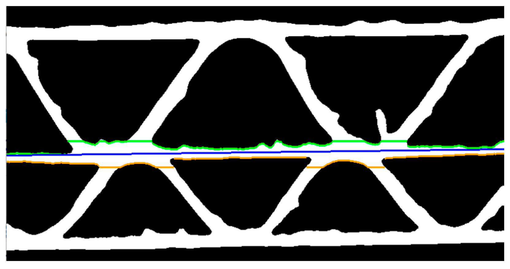
Figure 10.
Graphic representation of liners and flutes thicknesses measurement approach – blue, orange and turquoise areas – regions for determination of the upper liner, middle and lower liners thicknesses. Regions for flutes thicknesses measurements are marked in pink and green.
Figure 10.
Graphic representation of liners and flutes thicknesses measurement approach – blue, orange and turquoise areas – regions for determination of the upper liner, middle and lower liners thicknesses. Regions for flutes thicknesses measurements are marked in pink and green.
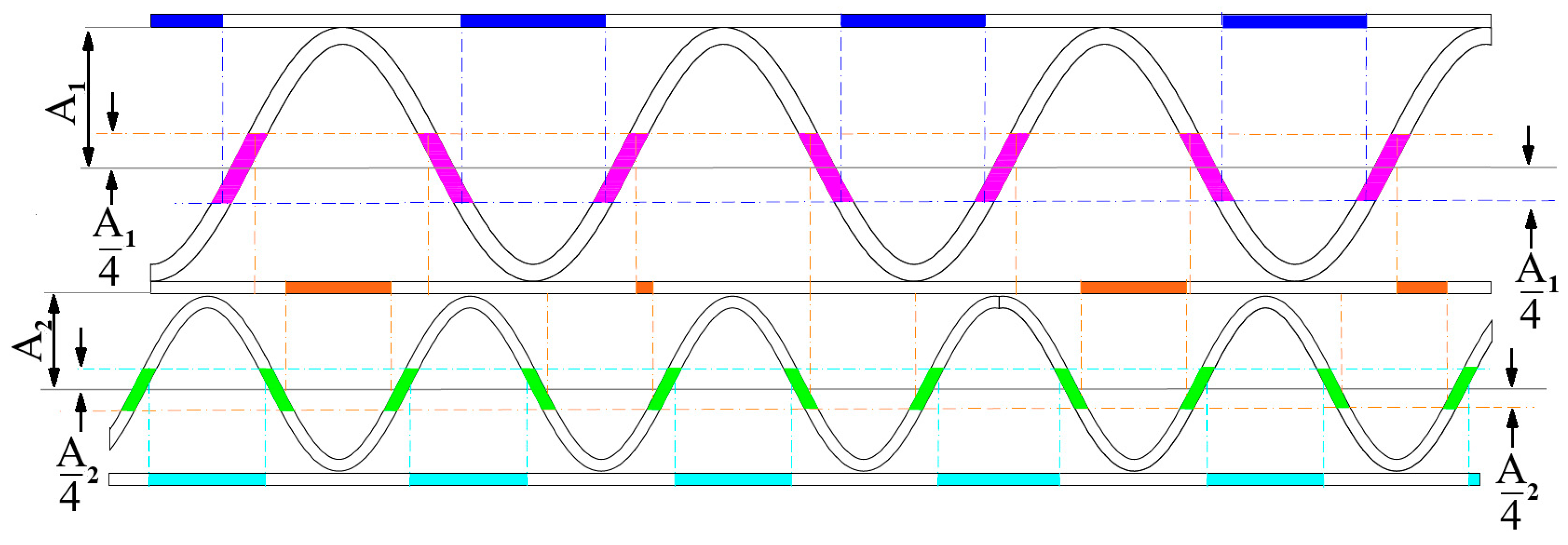
Figure 11.
An example of the results obtained by applying the proposed algorithm.
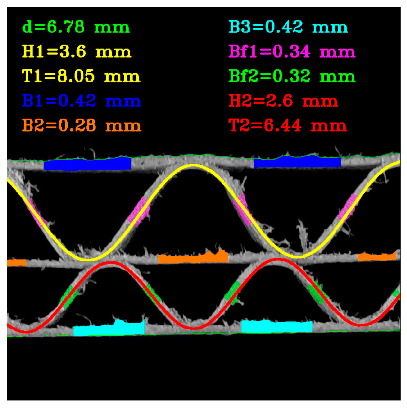
Figure 12.
Visualization of the recognized features of the corrugated board: (a) flute BC sample; (b) the results obtained for the flute BC sample; (c) flute EB sample; (d) the results obtained for the flute EB sample; (e) flute EC sample; (f) the results obtained for the flute EC sample; (g) flute EE sample; (h) the results obtained for the flute EE sample.
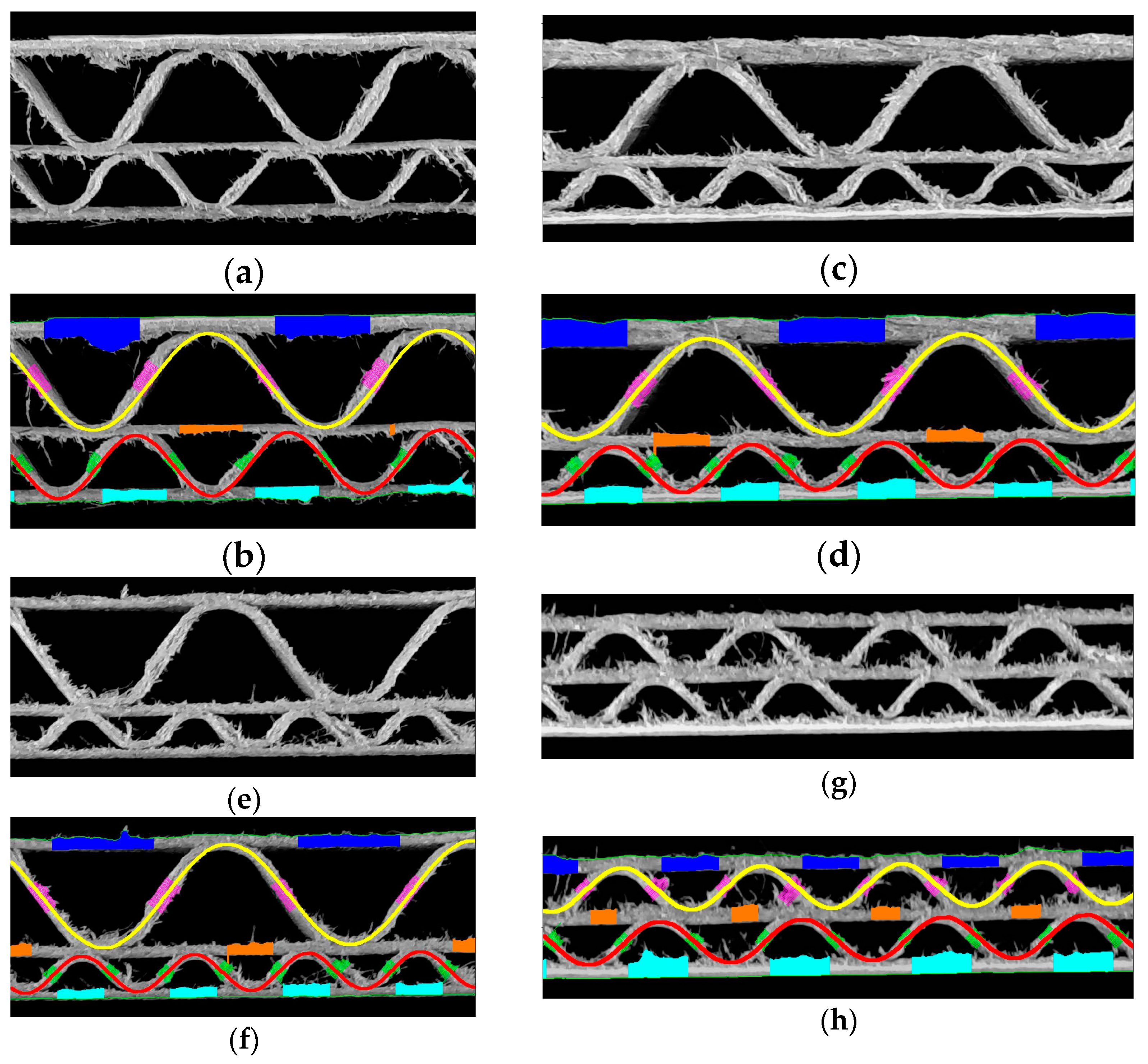
Figure 13.
Example of samples with BC flute: (a) a reference sample; (b) the results of identification for the reference sample; (c) a crushed sample with many jagged edges; (d) the results of identification for the crushed sample.
Figure 13.
Example of samples with BC flute: (a) a reference sample; (b) the results of identification for the reference sample; (c) a crushed sample with many jagged edges; (d) the results of identification for the crushed sample.
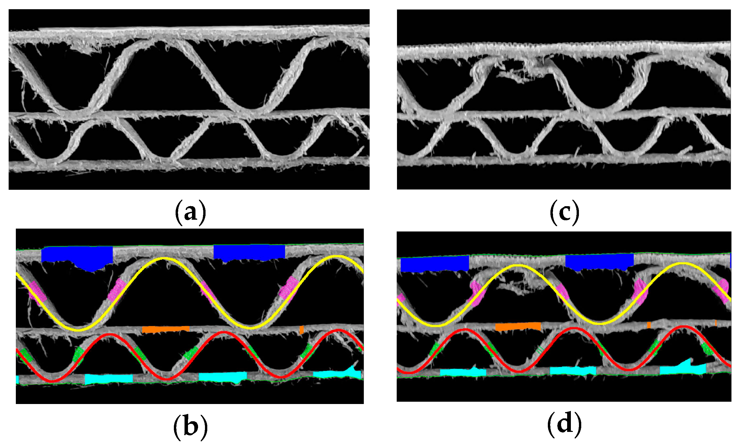
Figure 14.
Flute EB example: (a) a cardboard without damage; (b) the results of geometrical features identification for the sample without damage; (c) a damaged sample; (d) the results of geometrical features identification for the damaged sample.
Figure 14.
Flute EB example: (a) a cardboard without damage; (b) the results of geometrical features identification for the sample without damage; (c) a damaged sample; (d) the results of geometrical features identification for the damaged sample.
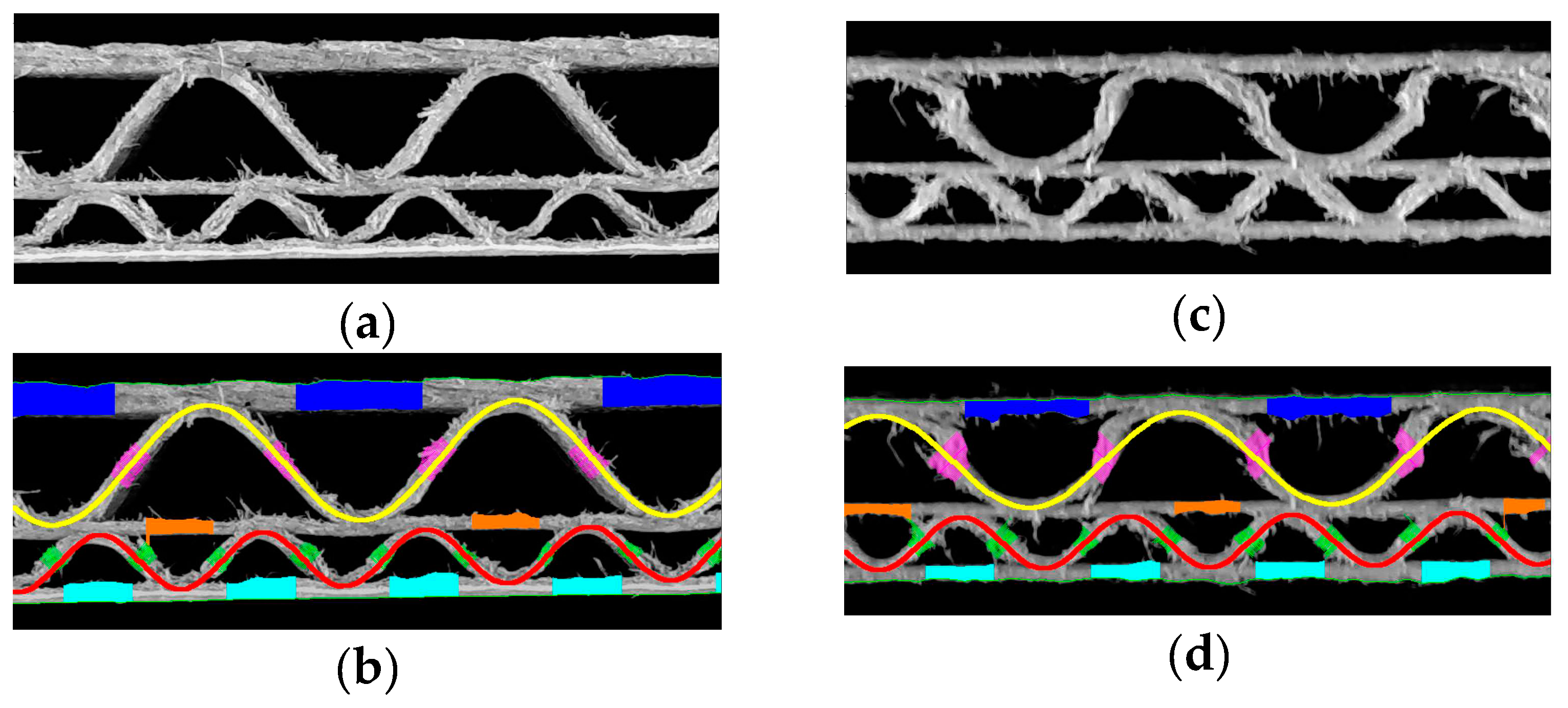
Figure 15.
Example of samples with EC flute: (a) a reference sample; (b) the results of identification for the reference sample; (c) a crushed sample with many jagged edges; (d) the results of identification for the crushed sample.
Figure 15.
Example of samples with EC flute: (a) a reference sample; (b) the results of identification for the reference sample; (c) a crushed sample with many jagged edges; (d) the results of identification for the crushed sample.
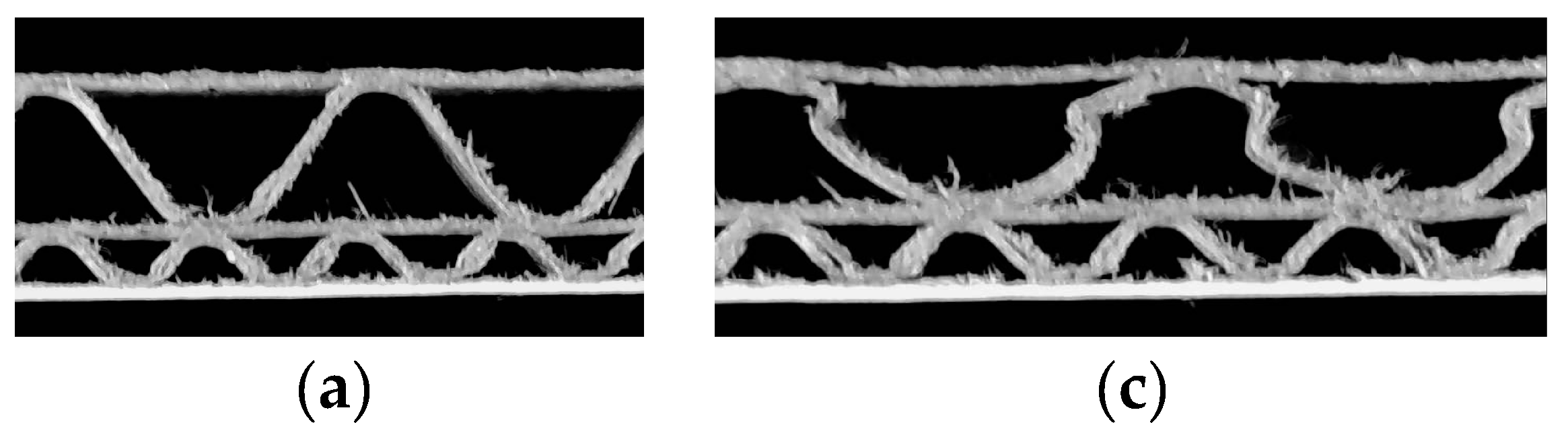
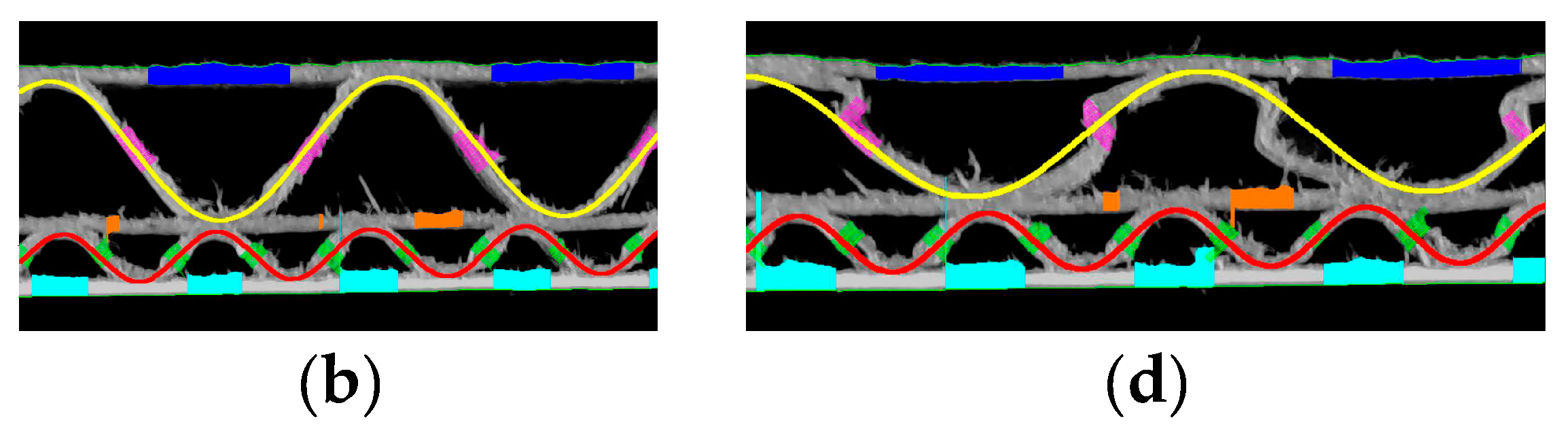
Figure 16.
Flute EE example: (a) a reference sample; (b) the results of identification for the reference sample; (c) a damaged sample; (d) the results of identification for the damaged sample.
Figure 16.
Flute EE example: (a) a reference sample; (b) the results of identification for the reference sample; (c) a damaged sample; (d) the results of identification for the damaged sample.
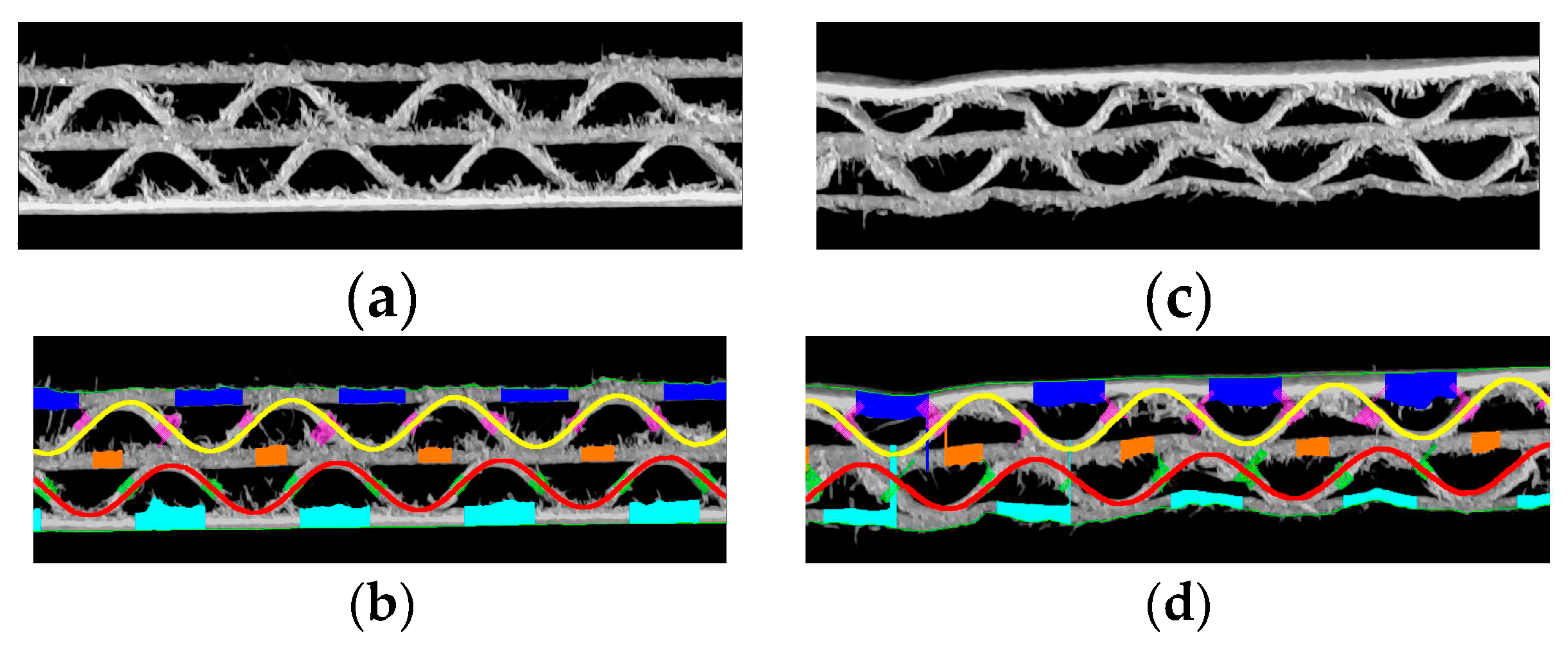
Figure 18.
Error in the measurements of the middle liner thickness due to in-phase composition of the corrugated layers: (a) flute EE sample; (b) incomplete results obtained for the EE flute sample.
Figure 18.
Error in the measurements of the middle liner thickness due to in-phase composition of the corrugated layers: (a) flute EE sample; (b) incomplete results obtained for the EE flute sample.
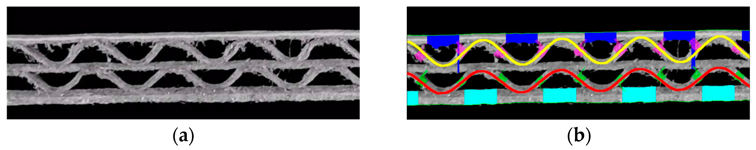

Table 1.
Identification results of the geometrical features for the corrugated boards with flutes BC, EB, EC and EE.
Table 1.
Identification results of the geometrical features for the corrugated boards with flutes BC, EB, EC and EE.
| Flute BC | Flute EB | Flute EC | Flute EE | |||||
|---|---|---|---|---|---|---|---|---|
| [px] | [mm] | [px] | [mm] | [px] | [mm] | [px] | [mm] | |
| height | 165 | 3.13 | 133 | 2.53 | 175 | 3.34 | 59 | 1.12 |
| period | 396 | 7.48 | 347 | 6.56 | 423 | 7.99 | 190 | 3.59 |
| height | 107 | 2.03 | 64 | 1.22 | 64 | 1.22 | 58 | 1.1 |
| period | 265 | 5.01 | 184 | 3.48 | 194 | 3.67 | 192 | 3.63 |
| Board thickness | 312 | 5.93 | 245 | 4.66 | 276 | 5.24 | 161 | 3.06 |
| Upper liner thickness | 39 | 0.74 | 33 | 0.63 | 20 | 0.38 | 18 | 0.34 |
| Middle liner thickness | 12 | 0.23 | 15 | 0.28 | 19 | 0.36 | 18 | 0.34 |
| Bottom liner thickness | 17 | 0.32 | 21 | 0.4 | 17 | 0.32 | 25 | 0.47 |
| thickness | 22 | 0.42 | 19 | 0.36 | 20 | 0.38 | 16 | 0.30 |
| thickness | 17 | 0.32 | 17 | 0.32 | 20 | 0.38 | 13 | 0.25 |
Table 2.
Identification results of the geometrical features for the corrugated board with flute BC (reference and crushed samples).
Table 2.
Identification results of the geometrical features for the corrugated board with flute BC (reference and crushed samples).
| Flute BC (Reference) | Flute BC (Crushed) | |||
|---|---|---|---|---|
| [px] | [mm] | [px] | [mm] | |
| height | 165 | 3.13 | 144 | 2.74 |
| period | 396 | 7.48 | 393 | 7.43 |
| height | 107 | 2.03 | 104 | 1.98 |
| period | 265 | 5.01 | 262 | 4.95 |
| Board thickness | 312 | 5.93 | 286 | 5.43 |
| Upper liner thickness | 39 | 0.74 | 35 | 0.67 |
| Middle liner thickness | 12 | 0.23 | 15 | 0.28 |
| Bottom liner thickness | 17 | 0.32 | 18 | 0.34 |
| thickness | 22 | 0.42 | 23 | 0.44 |
| thickness | 17 | 0.32 | 15 | 0.28 |
Table 3.
Identification results of the geometrical features for the corrugated board with flute EB (reference and crushed samples).
Table 3.
Identification results of the geometrical features for the corrugated board with flute EB (reference and crushed samples).
| Flute EB (Reference) | Flute EB (Crushed) | |||
|---|---|---|---|---|
| [px] | [mm] | [px] | [mm] | |
| height | 133 | 2.53 | 107 | 2.03 |
| period | 347 | 6.56 | 343 | 6.48 |
| height | 64 | 1.22 | 60 | 1.14 |
| period | 184 | 3.48 | 190 | 3.59 |
| Board thickness | 245 | 4.66 | 206 | 3.91 |
| Upper liner thickness | 33 | 0.63 | 20 | 0.38 |
| Middle liner thickness | 15 | 0.28 | 12 | 0.23 |
| Bottom liner thickness | 21 | 0.4 | 17 | 0.32 |
| thickness | 19 | 0.36 | 24 | 0.46 |
| thickness | 17 | 0.32 | 19 | 0.36 |
Table 4.
Identification results of the geometrical features for the corrugated board with flute EC (reference and crushed samples).
Table 4.
Identification results of the geometrical features for the corrugated board with flute EC (reference and crushed samples).
| Flute EC (Reference) | Flute EC (Crushed) | |||
|---|---|---|---|---|
| [px] | [mm] | [px] | [mm] | |
| height | 177 | 3.36 | 124 | 2.36 |
| period | 430 | 8.13 | 456 | 8.62 |
| height | 62 | 1.18 | 59 | 1.12 |
| period | 193 | 3.65 | 189 | 3.57 |
| Board thickness | 284 | 5.4 | 226 | 4.29 |
| Upper liner thickness | 22 | 0.42 | 16 | 0.30 |
| Middle liner thickness | 19 | 0.36 | 20 | 0.38 |
| Bottom liner thickness | 25 | 0.47 | 26 | 0.49 |
| thickness | 20 | 0.38 | 20 | 0.38 |
| thickness | 19 | 0.36 | 20 | 0.38 |
Table 5.
Identification results of the geometrical features for the corrugated board with flute EE (reference and crushed samples).
Table 5.
Identification results of the geometrical features for the corrugated board with flute EE (reference and crushed samples).
| Flute EE (Reference) | Flute EE (Crushed) | |||
|---|---|---|---|---|
| [px] | [mm] | [px] | [mm] | |
| height | 59 | 1.12 | 62 | 1.18 |
| period | 192 | 3.63 | 189 | 3.57 |
| height | 58 | 1.1 | 52 | 0.99 |
| period | 191 | 3.61 | 186 | 3.52 |
| Board thickness | 161 | 3.06 | 146 | 2.77 |
| Upper liner thickness | 18 | 0.34 | 29 | 0.55 |
| Middle liner thickness | 18 | 0.34 | 20 | 0.38 |
| Bottom liner thickness | 25 | 0.47 | 15 | 0.28 |
| thickness | 16 | 0.30 | 19 | 0.36 |
| thickness | 13 | 0.25 | 16 | 0.30 |
Disclaimer/Publisher’s Note: The statements, opinions and data contained in all publications are solely those of the individual author(s) and contributor(s) and not of MDPI and/or the editor(s). MDPI and/or the editor(s) disclaim responsibility for any injury to people or property resulting from any ideas, methods, instructions or products referred to in the content. |
© 2024 by the authors. Licensee MDPI, Basel, Switzerland. This article is an open access article distributed under the terms and conditions of the Creative Commons Attribution (CC BY) license (http://creativecommons.org/licenses/by/4.0/).
Copyright: This open access article is published under a Creative Commons CC BY 4.0 license, which permit the free download, distribution, and reuse, provided that the author and preprint are cited in any reuse.


