

Submitted:
22 January 2024
Posted:
23 January 2024
You are already at the latest version
Abstract
In the present article, the application of an artificial neural network (ANN) model is studied, whose function is the development of plastic instability maps of a medium carbon microalloyed steel during the hot forging process. And, secondly, we proceed to create another neural network capable of providing the recrystallized grain size in the steady state phase resulting from the deformation by hot forging, thus creating a methodology that can be applied to different types of processes and materials.
In order to achieve this objective, we start from the experimental data of a medium carbon microalloy steel, obtained by hot compression tests, for strain rates that vary between 10-4 and 3 s-1 and in a range of temperatures between 900 oC and 1150 oC. These experimental data will be used to train the neural network that is intended to be created in this work. Once trained, it will be verified if the results of the test correspond to the experimental data and the fluency curves will be obtained. Finally, the processing maps will be developed applying the Dynamic Materials Model (DMM), according to which the safe domains to forge the material and the plastic instability domains are delineated, to be avoided during the forging process. The maps obtained by means of RNA will be compared with the experimental ones and it will be possible to verify that the optimal regions of forging in the maps obtained by RNA coincide with those obtained by means of experimental data. In addition, a study of the influence of the microstructure on the behavior of steel during hot forming will be carried out, since the experimental tests are carried out at austenitizing temperature, so the microstructure is different in each test.
Keywords:
Red neuronal artificial
; modelo de material dinámico
; Procesamiento de mapas
; Comportamiento del flujo
; Acero microaleado de medio carbono
1. Introduction
The dynamic materials model (DMM) [1,2,3,4,5] is a method capable of characterizing hot forming work processes by analyzing and optimizing the hot formability of numerous materials. In the DMM, to characterize the creep behavior of materials, the potential constitutive law () is used, both in low and high stress domains. But, in the works published by Narayana Murthy et al. [6,7,8,9], it has been shown that the potential constitutive law cannot be used indiscriminately, at low and high voltages. It is known that said law can only be used in the analysis of steady-state stresses under low-stress forming conditions. For this reason, Narayana Murty et al. reanalyzed the DMM and proposed another methodology based on directly obtaining the energy dissipation efficiency through numerical integration, at any yield stress. This methodology can be considered as a variant of the DMM (VDMM). In these two methodologies, in order to achieve the optimal hot forming zones and, consequently, healthy parts without microstructural defects (cracks, fissures, cavities, etc.), it is necessary to skilfully and accurately apply the DMM and VDMM, analyzing the evolution of yield stress as a function of temperature and strain rate.
Another important parameter to take into consideration is the initial grain size because the microstructure of a shaped material is very sensitive to this parameter. Numerous studies have confirmed that the final microstructure resulting from microstructural evolution in the course of the hot-forming process has a decisive effect on the wear properties of the shaped part.
In the present work, in addition to the temperature, strain and strain rate, the initial grain size will be introduced as input data and control parameter for the development of a neural network capable of characterizing the hot forming of the material studied here [10].
Artificial neural networks (RNA) are hardware and/or software constructions that take input information and transform it into an output, generally applying a non-linear operation. They are simplified calculation models inspired by biological neural networks of the human brain. An RNA consists of a number of interconnected processing elements (perceptrons) called neurons. Neurons are organized in different layers, in ways similar to those in the human brain [11]. The processing elements of the neural network are distributed by layers. In each layer are the set of elements that are on the same level of the structure. The layers are as follows: input layer, intermediate layer, and output layer. There are three phases in the applications of neural networks:
– Learning phase: also called training phase. The ability to learn is a characteristic of neural networks. They learn by updating or changing the synaptic weights that characterize the connections. The weights are adapted according to the information extracted from the new training patterns that are presented. Normally, optimal weights are obtained by maximizing or minimizing some energy function. In supervised training, the mean square error (mse) between the master value and the current output value is usually minimized. During the learning process, the weights of the network connections undergo modifications; it can be affirmed that the process ends (the network has learned) when the values of the weights remain stable (dwij/dt=0).
– Test phase: once a model has been trained, it will be used in the test phase, in which the test patterns that constitute the usual input of the network are processed, analyzing the final features of the network. Once the network weights have been calculated, the values of the neurons in the last layer are compared with the desired output to determine the validity of the training.
– Validation or test phase: after training the weights of the connections remain fixed. We must check if the neural network can solve new problems, for which it has been trained. To validate the network, a data set is required, called the validation or test set.
Recently, artificial neural networks (RNA) have been used as a useful means to describe the creep behavior of a material under different conditions of temperature, strain, and strain rate. Many authors [12,13,14,15] use neural networks as a robust tool capable of predicting creep curves for each temperature, strain, and strain rate. The discrepancies basically in the treatment of data reside in the architecture of the network, such as: input variables used, range of values used for these input variables, number of hidden layers, number of neurons, transfer functions, activation and the initialization of the weights. On the other hand, they practically agree that the output variable, the yield stress, uses a multilayer perceptron network (MLP), based on Feed-Forward and with the retropropagation (BP) learning algorithm. Training stops when the Mean Squared Error (mse) is reached.
2. Experimental procedure
The commercial medium carbon microalloyed steel studied is intended for the forging sector for automotive components, and its chemical composition is represented in Table I.
| Table I.- Chemical composition of the studied. |
| %C %Mn %Si %P %S %V %Ti %Al Nppm |
| 0,29 1,19 0,19 0,012 0,025 0,09 0,002 0,011 131 |
The experimental method used to obtain the yield stress experimental data is the same used in previous publications [16], with the only difference being that the experimental tests have been carried out with prior austenitization for 30 min at test temperature. Therefore, the initial grain size, at each deformation temperature, is different. It should also be noted that a different alloy corresponds to each temperature, since the amount of elements put into solution or precipitated is also different at each test temperature.
To study the evolution of the initial grain size with time and temperature, austenitization treatments were carried out at different temperatures between 1150ºC and 900ºC and for a fixed holding time of 30 minutes. Figure 1 shows the initial microstructure of the studied steel austenized for 30 min at some test temperatures (900º-1050ºC and 1150º)[16].
The austenitizing treatments were carried out in a tube furnace capable of reaching 1500ºC, and in a protective atmosphere of argon to avoid possible decarburization. The specimens were introduced directly into the furnace when it reached the test temperature. The holding time began when the oven stabilized its temperature again, that is, between 30 and 45 seconds. after the specimen was placed in the furnace. Once the austenitization was finished, direct quenching was carried out in water at room temperature. Once the heat treatment was carried out, the metallographic preparation of the specimen was carried out for a subsequent measurement of the austenitic grain size.
2.1. Experimental data
Table II contains the experimental data of the yield stress, for different temperatures, strains and strain rates, used for the construction of the neural network.
| Table II.- Experimental data of the experimental yield stress for different temperatures, strains and strain rates Microalloyed steel M-30 | |
| Tº (ºC) | Strain rates() (s-1) |
| 900º | 1E-4, 5E-4, 1E-3, 2E-3, 3E-3, 5E-3, 1E-2, 2E-2, 3E-2, 5E-2,7E-2 |
| 950º | 2E-4, 5E-4, 1E-3, 2E-3, 5E-3, 1E-2, 2E-2, 5E-2, 1E-1, 1, 3 |
| 1000º | 1E-4, 2E-4, 5E-4, 6E-4, 7E-4, 1E-3, 2E-3, 5E-3, 1E-2, 2E-2, 5E-2, 1E-1, 1, 3 |
| 1050º | 1E-4, 5E-4, 1E-3, 5E-3, 1E-2, 2E-2, 5E-2, 1E-1, 1, 3 |
| 1100º | 1E-4, 2E-4, 3E-4, 5E-4, 1E-3, 3E-3, 1E-2, 2E-2, 3E-2, 1E-1, 1,3 |
| 1150º | 1,3 |
3. Neural network model to obtain the processing maps
3.1. Data preparation
In order to correctly use the experimental results, it is necessary to carry out an efficient data treatment, in order to create a methodology capable of obtaining the maximum performance from them and, consequently, facilitate their application in neural networks, both in the learning phase as well as the testing and validation phases. A correct selection will mean greater goodness in the final results. In this work, a large quantity and variety of experimental data is available (see Table III) which requires unifying the selection criteria thereof. In order to create a database that facilitates the application of the neural network model, both the input data (inputs) and the output data (outputs) are treated adopting the following rules: the fluency curves used, the microalloyed steel studied, both for training and validation of the network, are those that correspond to the main strain rates, that is, from 1E-4 s-1, 1E-3 s-1, 1E-2 s-1, 1E-1 s-1, 1 s-1 and 3 s-1, since they are curves whose experimental data is repeated at most of the temperatures studied. The intermediate strain rates are used for the test. In addition, since the neural network requires that both the input and output data must be between 0 and 1 and in order to accelerate the convergence in the learning rate, we are interested in the data having small values, so that we ensure the settlement of the network in a solution. First, for T, and the logarithms of the experimental values are used, and then they are normalized [28] between 0 and 1. For T and σ the following equation is applied:
where Z are the experimental data (T and σ) in logarithms, Z’ is the normalized value of Z, which has a maximum and minimum value given by Zmax and Zmin, respectively.
However, the above equation (1) cannot be used to normalize, the values obtained are too small. To normalize the values of the following equation is used:
Being the experimental value, and the normalized value of. In formula (2), the value 5 is used so that all normalized values are positive. This value will depend on the minimum deformation speed that we have in the experimental data of the steel. However, it is not necessary to normalize the deformation ε since its values are between 0 and 1.
The experimental data used to train and test the network are presented in Table III. The data used for training is 726 (55%), for validation 198 (15%) and for testing 1296 (30%).
| Table III: Experimental data used from M-30 steel for ANN Training and Testing |
| (s-1) Training (M-30) Testing |
| 1E-4 900,1000,1100 ºC 1050 ºC |
| 1E-3 900,1000,1050,1100 ºC 950 ºC |
| 1E-2 900,950,1050,1100 ºC 1000 ºC |
| 1E-1 950,1000,1100 ºC |
| 1 950,1050,1100,1150 ºC 1000 ºC |
| 3 950,1000,1050,1150 ºC 1100 ºC |
The yield stress results obtained by validating or testing the network make it possible to define its reliability. These values will be those that correspond to the temperatures, strains and strain rates that have not been used for training and testing. Table IV represents the data used to verify the ANN validation test.
| Table IV: Experimental data of the M-30 steel used for the ANN validation |
| (s-1) Validation |
| 3E-3 900 ºC |
| 5E-3 950 ºC |
| 5E-4 950 ºC, 1000 ºC,1050 ºC,1100 ºC |
3.2.1. Neural network model
The network model used is the Multilayer Perceptron or MLP (Multi-Layer Perceptron) based on Feed-Forward and backpropagation (BP) has been used as a supervised learning algorithm. For training, the Levenberg-Marquardt algorithm (trainlm) based on backpropagation is applied. The weights are chosen at random, the network itself determines the weights randomly. The transfer and activation function is sigmoidal:
The number of hidden layers, with their neurons, and the minimum square error (MSE) that will determine the highest efficiency in the results, for each steel, is obtained from the standard statistical data resulting from training and testing. Then the final verification tests are carried out.
The architecture of the network that we adopt is made up of three layers, an input layer made up of three elements (T, ε,), two hidden layers with twelve and nine neurons, and the voltage (σ) as the output layer. The architecture of the network, 3-12-9-1, is represented in Figure 2. The best results are obtained for a minimum square error (MSE) of 0,00007. Training stops after 224 iterations.
3.2.2. Standard validation of the results of the Neural Network
After the training of the network, the performance of the network is checked for the test curves and the results obtained must be validated. A number of standard statistical methods are used to assess validity [17,18,19]. These methods are able to show the generalization capacity of network formation. It is quantified in terms of the correlation coefficient (R), the average relative absolute error (eAARE), the square root of the mean square error (RMSE), the dispersion index (SI) and the relative error (error between the experimental data) and those obtained by RNA. These parameters are defined below:
where E is the experimental value and P is the value obtained using the neural network model; and are the mean values of E and P, respectively; N is the total number of data used in the investigation; p corresponds to the number of output variables.
It is well known that small values (zero approximation) of AARE and RMSE signify a good correlation between predictive and experimental data. But, it is important to note that the highest values of coefficient R (close to 1) should not always be interpreted as evidence of a good predictive performance of the developed RNA model, because these values do not fully describe the relationship between the experimental values. and those predicted [20,21]. However, to evaluate the RNA model, standard statistical indices are used. Table V contains the statistical results of the network model used:
| Table V: RNA model performance for training, testing and validation |
| R RMSE(%) AARE(%) SI |
| Trainig 0,99781 2,8974 3,5978 0,0007 |
| Test 0,99059 3,5909 4,3209 0,0553 |
| Validation 0,99377 4,1508 4,7632 0,0637 |
The error distribution of the yield stress of the neural network model in relation to the experimental data is shown in Figure 3.
As can be seen graphically in Figure 3, the values of the tension in the training, test and validation of the ANN reveal that they are very similar to the experimental ones. Most of the points fall along the 45º line, and the correlation coefficients for training, test, and validation are 0.99781, 0,99059, and 0,99377, respectively. All the above results indicate that the RNA model has been successfully trained and can be applied to predict the flow stress behavior of M-30 steel.
To confirm the accuracy of the RNA model performance, statistical analysis of the relative error is also used. The distribution of the prediction error of the RNA model for the training, test and validation is shown in Figure 4. This figure indicates that the predictions of the relative errors of the three data sets show a typical Gaussian distribution and show that are within 10% for more than 95% of the test data (a relative error of 5% is observed for more than 85% of the training data). Consequently, the good performance in the prediction of the proposed RNA model is confirmed.
3.3. Application of the dynamic model of materials
3.3.1. Flow curves
The creep curves for the steels are represented in Figure 5, Figure 6, Figure 7 and Figure 8. In them it is possible to observe the evolution of the true stress as a function of the true deformation, both for the experimental curves (in black) and for those obtained by ANN (in red).
The main characteristics of the experimental creep curves are those typical of materials that undergo restoration and dynamic recrystallization, and the same can be said for the curves obtained through the neural network. The maximum peak stress σp and the peak strain εp increase with strain rate, for a given temperature. As the temperature increases, σp and εp decrease.
It can be seen that the proposed RNA model gives, under different deformation conditions, an accurate estimate of the yield curves of the studied steel and the results are very similar.
3.3.2. Experimental processing maps obtained by DMM and VDMM
In the research work carried out by Al Omar [16], the processing maps (energy dissipation efficiency maps and plastic instabilities maps) of the studied steel obtained using the DMM are represented. The energy dissipation efficiency map reveals the existence of two domains characterized by maximum efficiency. The first domain occurs in the region of low temperatures and moderate strain rates (centered at approximately 900 °C and 0,0001 s-1). In this case of low temperatures and intermediate strain rates, it is to be expected that the DRV will act; typical creep curves within this domain are characteristic of DRV. In a hot forming process, both DRX and DRV are considered beneficial mechanisms for the microstructure and consequently the mechanical properties of the formed material, as they provide stable flow and improve the formability of the material [17,21]. The second domain appears centered at 1100 °C and 1 s−1 with a maximum efficiency of approximately 31%; it is the domain of DRX. This correlation is confirmed by the creep curves obtained under different combinations of temperature and strain rate in this domain and clearly show continuous softening with single peak behaviour. For temperatures between 900-950ºC and high deformation speeds, a domain with low efficiency values appears that can be identified with zones that are not suitable for forming the material studied [22].
In relation to the plastic instability [22] map based on the DMM, as is known, the greater the negative magnitude of the plastic instability parameter ξ, the greater the possibility of the appearance of some manifestation of plastic instability [37]. Thus, in order to always form under stable flow conditions, domains of possible instabilities must be avoided during hot forming processes. The map represents two zones of stability; one for a temperature of 900ºC and a strain rate of 0,0001 s-1 and the other for 1100ºC at 3 s-1.
In Figure 9, the processing maps based on VDMM are represented. These maps reveal a domain of plastic instability between 900-950ºC and high strain rates of 3 s-1, this domain coincides with the domain found in the DMM maps. Despite the small difference found in the position of the stable domains, a good agreement has been observed between the different processing maps built based on the two models, the DMM and the VDMM.
3.4. Application of ANN to develop processing maps
To check the reliability of the ANN proposed in this work, processing maps were built, based on the DMM (Figure 10) and on the VDMM (Figure 11), using the flow curves obtained by the ANN. These maps coincide with the same domains as those obtained through the experimental stress-strain curves applying the DMM and VDMM models.
The DRX domain appears at 1100ºC and 3 s-1 with an approximate efficiency of 32% and another DRV domain appears at low temperatures and strain rates, centered approximately at 900ºC and 0.0001 s-1. In addition, an instability domain appears at low temperatures and high strain rates (900ºC and 3 s-1) with very low efficiency and it would be convenient not to conform under these conditions.
The similarity between the experimental processing maps and those obtained using ANN suggest, for future research, that the ANN developed in this work can be implemented in a commercial finite element code to more efficiently simulate the hot flow behavior of medium carbon microalloyed steels.
4. RNA to obtain the recrystallized grain size
4.1. Experimental data on grain size
Table VI represents the experimental data of the initial grain size and the final grain size at deformation of 0,6, corresponding to the stable state, for different temperatures and deformation speeds.
| Table VI. Experimental initial and final grain size for different temperatures and strain rates |
| T (ºC) (s-1) GS.INITIAL (μm) GS.FINAL (μm) |
| 900 0,0001 11,12 22,2557 |
| 900 0,0005 11,12 14,81 |
| 900 0,0020 11,12 12,9680 |
| 900 0,0100 11,12 11,3415 |
| 900 0,0500 11,12 9,799 |
| 900 0,3000 11,12 8,3298 |
| 950 0,0002 12,63 33,9160 |
| 950 0,0005 12,63 26,6486 |
| 950 0,0010 12,63 21,0201 |
| 950 0,0050 12,63 16,8403 |
| 950 0,0100 12,63 15,8876 |
| 950 0,0500 12,63 13,967 |
| 950 0,3000 12,63 12,3852 |
| 1000 0,0001 21,1 95 |
| 1000 0,0002 21,1 76 |
| 1000 0,0007 21,1 52,4296 |
| 1000 0,0020 21,1 37,7328 |
| 1000 0,0100 21,1 27,9388 |
| 1000 0,0500 21,1 23,9435 |
| 1000 0,1000 21,1 22,6202 |
| 1000 0,3000 21,1 21,3700 |
| 1050 0,0001 77,57 164,8713 |
| 1050 0,0100 77,57 46,0404 |
| 1050 0,0200 77,57 40,4298 |
| 1050 0,0500 77,57 37,4276 |
| 1050 0,1000 77,57 36,2312 |
| 1050 0,3000 77,57 33,9519 |
| 1100 0,0001 117,79 253,4429 |
| 1100 0,0010 117,79 131,3201 |
| 1100 0,0100 117,79 70,5940 |
| 1100 0,0300 117,79 61,9280 |
| 1100 0,1000 117,79 53,9414 |
| 1100 0,3000 117,79 49,1312 |
4.2. Construction of the neural network model to obtain the grain size
In the same way as in the previously developed RNA model, temperature and strain rate were normalized for values between 0 and 1. Grain size values do not need to be normalized. The model is the same as the one previously developed used to determine the creep curves; that is, the Multilayer Perceptron or MLP (Multi-Layer Perceptron) based on Feed-Forward and backpropagation (BP) as a learning algorithm. For training, the Levenberg-Marquardt (TRAINLM) algorithm is applied, based on the backpropagation (BP) learning algorithm.
The network architecture we adopt is composed of three layers, input, test and validation. The input layer is composed of three elements (T,, Gs.Initial), two hidden layers with twelve and nine neurons, and as output layer it will be the Final Grain Size, recrystallized (Gs.Final). The architecture of the network, 3-11-6-1, is represented in Figure 12.
4.1. ANN results
Table VII shows the results obtained by ANN in training.
| Table VII.- Data obtained through ANN in training |
| T (ºC) (s-1) GS.INITIAL (μm) GS.FINAL (μm) ANN(μm) |
| 900 0,0001 11,12 22,2557 21,6098 |
| 900 0,0005 11,12 14,81 15,4256 |
| 900 0,0020 11,12 12,9680 11,1386 |
| 900 0,0500 11,12 9,799 9,8309 |
| 900 0,3000 11,12 8,3298 9,7824 |
| 950 0,0002 12,63 33,9160 33,4308 |
| 950 0,0005 12,63 26,6486 26,5033 |
| 950 0,0050 12,63 16,8403 16,6861 |
| 950 0,0100 12,63 15,8876 15,4176 |
| 950 0,0500 12,63 13,967 14,0240 |
| 950 0,3000 12,63 12,3852 12,2633 |
| 1000 0,0001 21,1 95 94,8702 |
| 1000 0,0007 21,1 52,4296 52,3033 |
| 1000 0,0020 21,1 37,7328 37,5001 |
| 1000 0,0100 21,1 27,9388 28,2090 |
| 1000 0,0500 21,1 23,9435 23,9700 |
| 1000 0,1000 21,1 22,6202 22,3469 |
| 1000 0,3000 21,1 21,3700 21,4938 |
| 1050 0,0001 77,57 164,8713 165,0638 |
| 1050 0,0100 77,57 46,0404 46,0867 |
| 1050 0,0200 77,57 40,4298 40,5404 |
| 1050 0,0500 77,57 37,4276 37,3475 |
| 1050 0,1000 77,57 36,2312 36,1864 |
| 1100 0,0001 117,79 253,4429 253,4109 |
| 1100 0,0010 117,79 131,3201 131,3422 |
| 1100 0,0100 117,79 70,5940 70,5405 |
| 1100 0,0300 117,79 61,9280 61,9516 |
| 1100 0,1000 117,79 53,9414 53,9305 |
| 1100 0,3000 117,79 49,1312 49,1622 |
The RNA results for the test are set forth in Table VIII.
| Table VIII.- Results of the RNA test | ||||
| Tº(ºC) | (s-1) | GS.FINAL (μm) | ANN(μm) | ERROR(%) |
| 900 | 0,0100 | 11,3416 | 9,8553 | 1,4863 |
| 950 | 0,0010 | 21,0201 | 21,9764 | -0,9563 |
| 1000 | 0,0002 | 76,0000 | 82,6071 | -6,6071 |
| 1000 | 0,0500 | 23,9436 | 23,9700 | -0,0265 |
| 1050 | 0,3000 | 33,9519 | 32,3338 | 1,6181 |
Because the available experimental data is very limited for the validation of the network, if we apply new inputs to the trained network to obtain the final grain sizes of all the main strain rates and some of which we do not have experimental results, with which we cannot compare the results we obtain with the results of Table IX.
| Table IX.-Results of the ANN validation | |||
| Tº(ºC) | (s-1) | GS.INITIAL (μm) | GS.FINAL(μm)ANN |
| 900 | 0,0001 | 11,12 | 21,6098 |
| 900 | 0,001 | 11,12 | 12,8276 |
| 900 | 0,01 | 11,12 | 9,8553 |
| 900 | 0,1 | 11,12 | 9,8426 |
| 950 | 0,0001 | 12,63 | 3,4371 |
| 950 | 0,001 | 12,63 | 21,9764 |
| 950 | 0,01 | 12,63 | 15,4176 |
| 950 | 0,1 | 12,63 | 12,848 |
| 1000 | 0,0001 | 21,1 | 94,8702 |
| 1000 | 0,001 | 21,1 | 45,5325 |
| 1000 | 0,01 | 21,1 | 28,209 |
| 1000 | 0,1 | 21,1 | 22,3469 |
| 1050 | 0,0001 | 77,57 | 165,0638 |
| 1050 | 0,001 | 77,57 | 83,6777 |
| 1050 | 0,01 | 77,57 | 46,0867 |
| 1050 | 0,1 | 77,57 | 36,1864 |
| 1100 | 0,0001 | 117,79 | 253,4109 |
| 1100 | 0,001 | 117,79 | 131,3422 |
| 1100 | 0,01 | 117,79 | 70,5405 |
| 1100 | 0,1 | 117,79 | 53,9305 |
The results obtained by ANN can be compared with the experimental results shown in Figure 13 and Figure 14. In these figures, it is clearly observed that in the range of high temperatures and very low deformation speeds there was grain growth and as it increases the speed of deformation the grain is refined. It should always be taken into account that in this case the initial grain size is different at each temperature.
Regardless of the theories that attempt to explain through nucleation and growth mechanisms during dynamic recrystallization, the existence of a grain refinement for single peak recrystallization is evident.
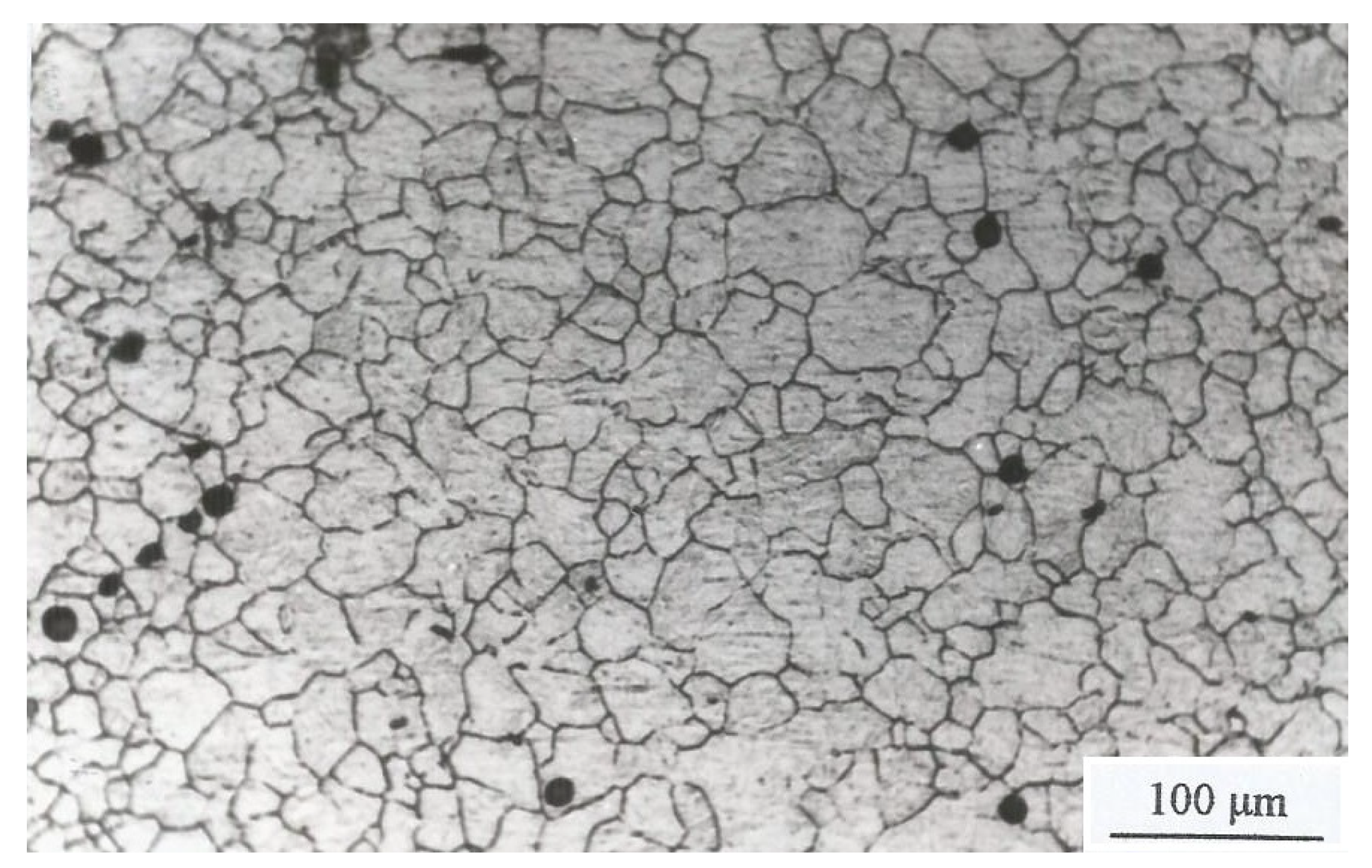
The interpretation of the domains that appear in the processing maps of the studied steel can be done using the creep curves associated with each domain, as well as the evolution of grain size with temperature and strain rate. Therefore, the broad domain, observed in the processing maps, located at low strain rates represents the single peak dynamic recrystallization in the temperature range 900 and 950 ºC, while at higher temperatures (950 ºC) this same domain it is representative of cyclic dynamic recrystallization. The domain located at high strain rates and high temperatures represents the process of single-peak dynamic recrystallization. The microstructure of the specimens deformed at T = 1100 ºC, = 0,3 s-1 is represented in Figure 15 [16]. It is noteworthy that in these microstructures considerable reconstitution of the microstructure due to dynamic recrystallization processes and perhaps also additional post-dynamic processes is evident.
5. Conclusions
Two artificial neural network (RNA) models are used successfully in this study. The first to develop the processing maps for a medium carbon microalloy steel, subjected to a hot forming process. The second model was developed to be able to determine the recrystallized grain size in steady state. The ANN is trained using temperature, strain, and strain rate as input data and yield stress as target or output data. The network model used is the MLP (Multi-Layer Perceptron) and backpropagation (BP) learning algorithm. For network training, the Levenberg-Marquardt (TRAINLM) algorithm is applied, based on the backpropagation (BP) learning algorithm. The processing maps of the studied steel were developed based on the dynamic materials model (DMM) and its variant (VDMM). In these maps it has been possible to define safe areas for forming and areas to avoid. These results are of great industrial interest because they allow choosing the most appropriate control parameters to carry out the forming process with full guarantees of success and reliability. The comparison between the experimental processing maps and those of the RNA show a very high similarity, which demonstrates the robustness and reliability of the RNA proposed in this work.
In relation to the RNA model proposed to determine the recrystallized grain size, the same method has been used as in the first RNA, with the difference that, in this case, very few data are available to train and validate the network. But, despite this, the ANN results are very close to the experimental ones, so it is considered that the training, testing and validation have been satisfactory. The graphs obtained in relation to the recrystallized grain size follow the trend of other studies carried out, so it can be confirmed that the results obtained using the proposed RNA are correct.
Artificial neural networks are an efficient method to simulate the yield stress behavior of materials subjected to hot forming processes to determine the control parameters necessary to carry out safe forming without plastic instabilities. In addition, this method allows predicting the evolution of the shaped microstructure, through the grain size.
The authors are grateful for the financial support received from the CICYT (Spain) through the research project competitive PID2020-114819GB-I00.
References
- Y.V.R.K. Prasad, T. Seshacharyulu: Int. Mater. Rev. 43 (1998) 243. [CrossRef]
- S.V.S. Narayana Murty, B. Nageswara, B.P. Kash: Int. Mater. Rev. 45 (2000) 15. [CrossRef]
- A.H. Sheikhali, M. Morakkabati: Int. J. Mater. Res. 111 (2020) 1. [CrossRef]
- E. Ghasemi, A. Zarei-Hanzaki, E. Farabi, K. Tesar, A. Jäger, M. Rezaee: J. Alloys Compd. 695 (2017) 1706. [CrossRef]
- Y.V.R.K. Prasad, K.P. Rao, S. Sasidhar: Hot Working Guide, MaterialsPark, OH: ASM International (2015).
- S.V.S. Narayana Murty and B. Nageswara Rao: Mater. Sci. Lett.17 (1998) 1203. [CrossRef]
- S.V.S. Narayana Murty, B. Nageswara Rao, B.P. Kashyap: Modell.Simul. Mater. Eng. 10 (2002) 503. [CrossRef]
- S.V.S. Narayana Murty, B. Nageswara Rao, B.P. Kashyap: Comput. Sci. Technol. 63 (2003) 119. [CrossRef]
- S.V.S. Narayana Murty, B. Nageswara Rao, B.P. Kashyap: J. Mater. Process. Technol. 166 (2005) 279. [CrossRef]
- McCulloch, W. and Pitts, W., 1943, “A logical calculus of the ideas immanent in nervous activity,” Bulletin of Mathematical Biophysics, 5, p 115-133.
- McCulloch, W. and Pitts, W., 1943, “A logical calculus of the ideas immanent in nervous activity,” Bulletin of Mathematical Biophysics, 5, p 115-133.
- M.P. Phaniraj, A.Kumar, The applicability of neural network model to predict flow stress for carbon steels. Journal of Materials Processing Technology 141 (2003) 219-227.
- Y. Sun, W. Zeng, Y. Zhao,X. Zhang, X. Ma, Y. Han. Constructing processin map of Ti40 alloy using artificial neural network. Sciencie Direct. Trans. Nonferrous Met. Soc. China 21 (2011) 159-165.
- Alcelay, I., Peña, E., Al Omar, A. (2016) “Estudio del comportamiento termo-mecánico de un acero microaleado de medio carbono durante un proceso de conformado en caliente usando una red neuronal artificial”. Rev. Metal. 52(2): e066. [CrossRef]
- I. Alcelay, Anas Al Omar, J. Manuel Prado. Characterization of hot flow behaviour and deformation stability of medium carbon microalloyed steel using artificial neural networks and dynamic material model Int. J. Mater. Res. (formerly Z. Metallkd.) 105 (2014) 8; page 743– 754.
- A. Al Omar: Doctoral Thesis, Universidad Politécnica de Cataluña, Barcelona, Spain (1996).
- José Ignacio Alcelay Larrión: Doctoral Thesis, Universidad Politécnica de Cataluña, Barcelona, Spain (2015).
- S. Mandal,P.V. Sivaprasad, S. Vegunopal. Capability of a Feed-Forward Artificial Neural Network to predict the constitutive flow behavior of as cast 304 stainless steel under hot deformation. Materials Technology Division, Indira Gandhi Centre for Atomic Research. Vol. 129, 2007.
- Gouliand Ji, Fugou Li, Qinghua Li, Huiqu Li, Zhi Li. Prediction of the hot deformation behavior for Aermet100 steel using an artificial neural network. Computational Materials Sciencie 48 (2010) 626-632.252.
- Y. Sun, W. Zeng, Y. Zhao,X. Zhang, X. Ma, Y. Han. Constructing processin map of Ti40 alloy using artificial neural network. Sciencie Direct. Trans. Nonferrous Met. Soc. China 21 (2011) 159-165.
- M.T.Hagan, H.B.Demuth and M. Beale, Neural Network Design, Thomson Learning, Singapore, 2002. (Error relative menor Levenberg marquard).
- Prasad, Y.V.R.K., Sasidhara S. (1997). Hot Working Guide: A Compendium of Processing Maps, ASM International, Materials Park, Ohio, USA.
Figure 1.
Initial microstructure 30 min. of M-30 steel: a) 900 ºC b) 1050 ºC and c) 1150 ºC.
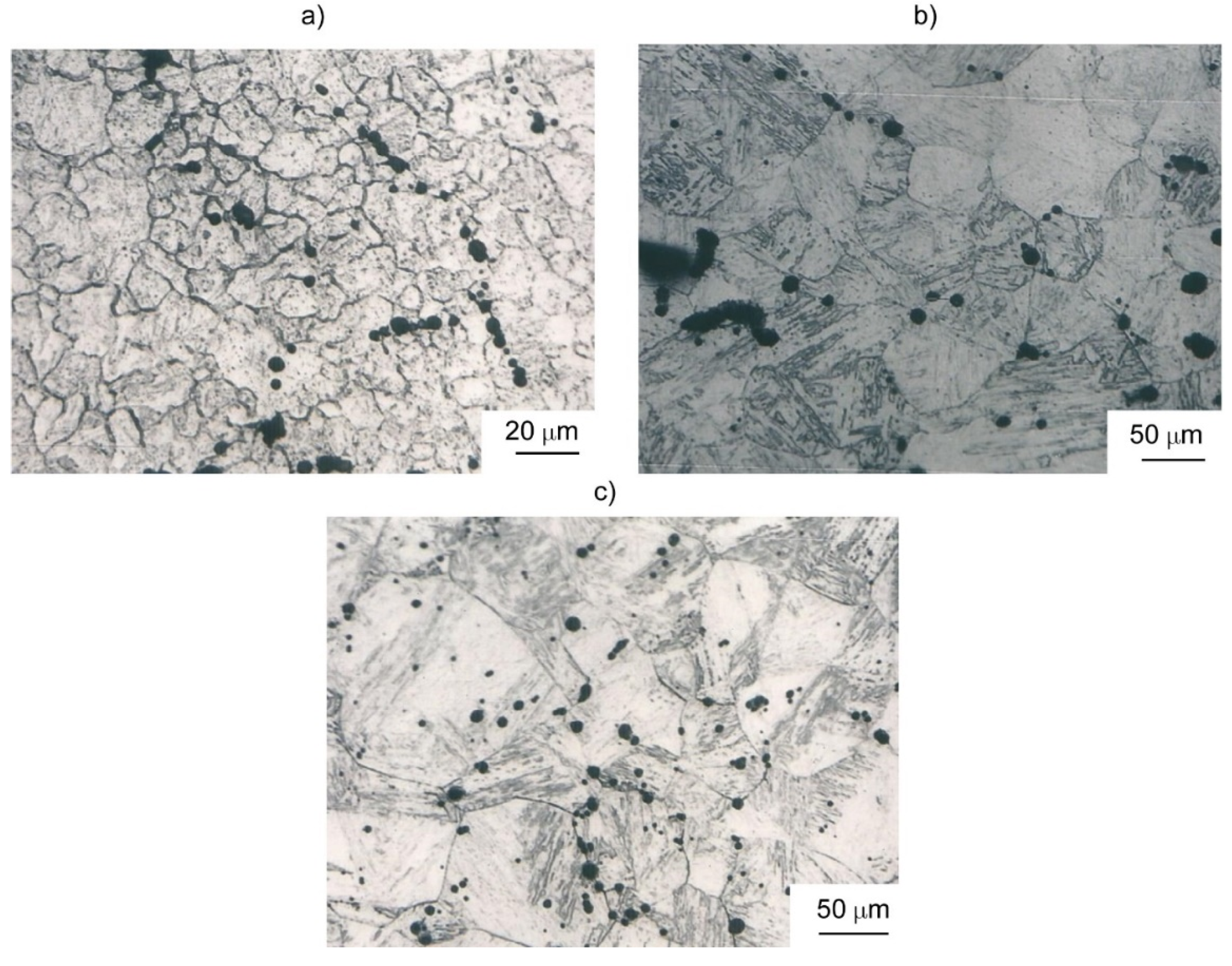
Figure 2.
ANN model.
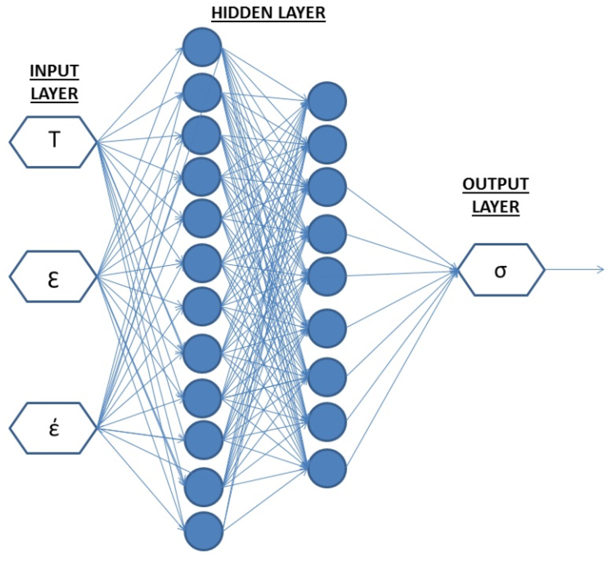
Figure 3.
Comparison between the experimental flow stress and that obtained by the ANN for M-30 steel: a) training b) test and c) validation.
Figure 3.
Comparison between the experimental flow stress and that obtained by the ANN for M-30 steel: a) training b) test and c) validation.
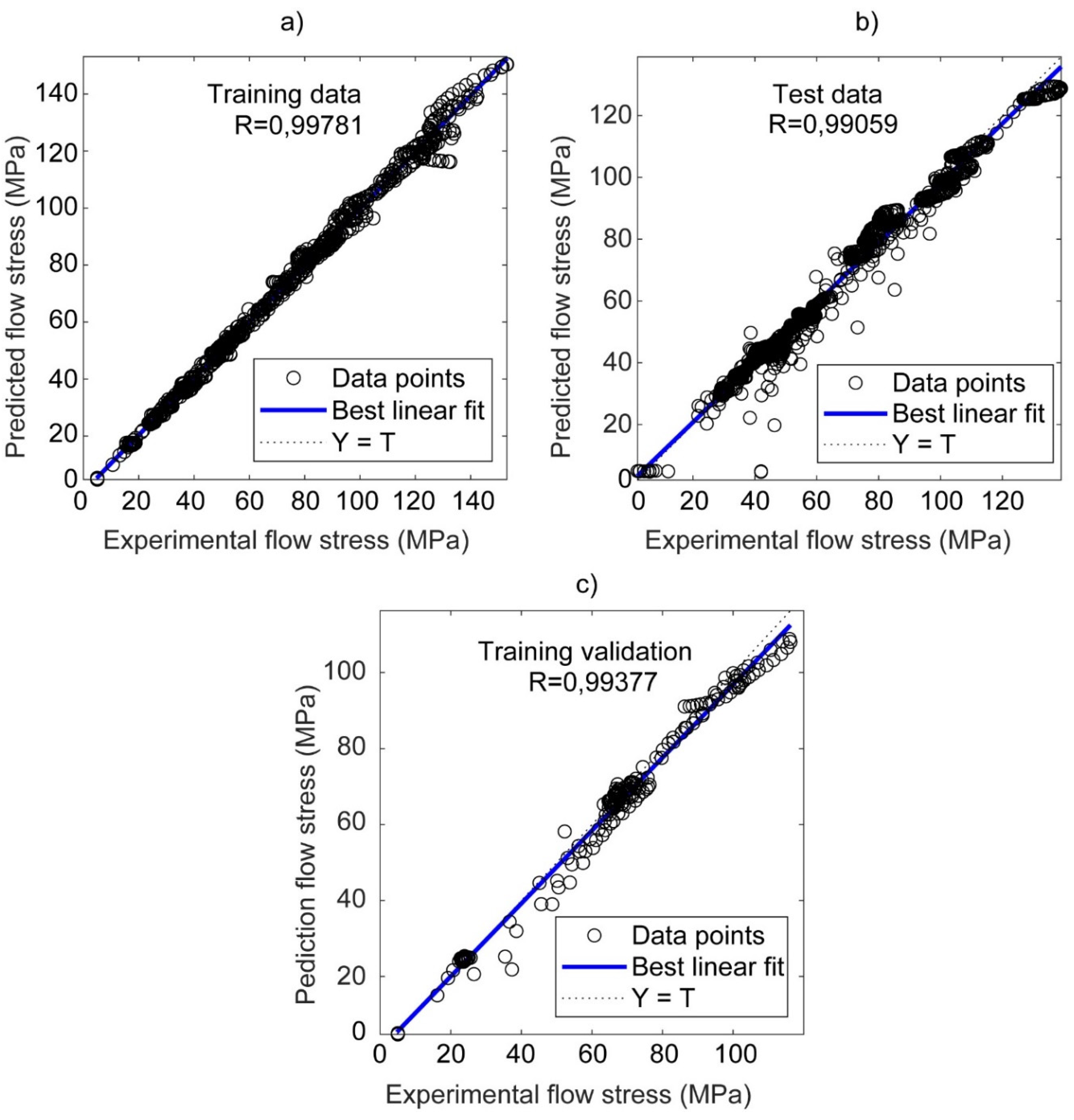
Figure 4.
Statistical analysis of the prediction error of the ANN model for M-30 steel: a) training b) test and c) validation.
Figure 4.
Statistical analysis of the prediction error of the ANN model for M-30 steel: a) training b) test and c) validation.
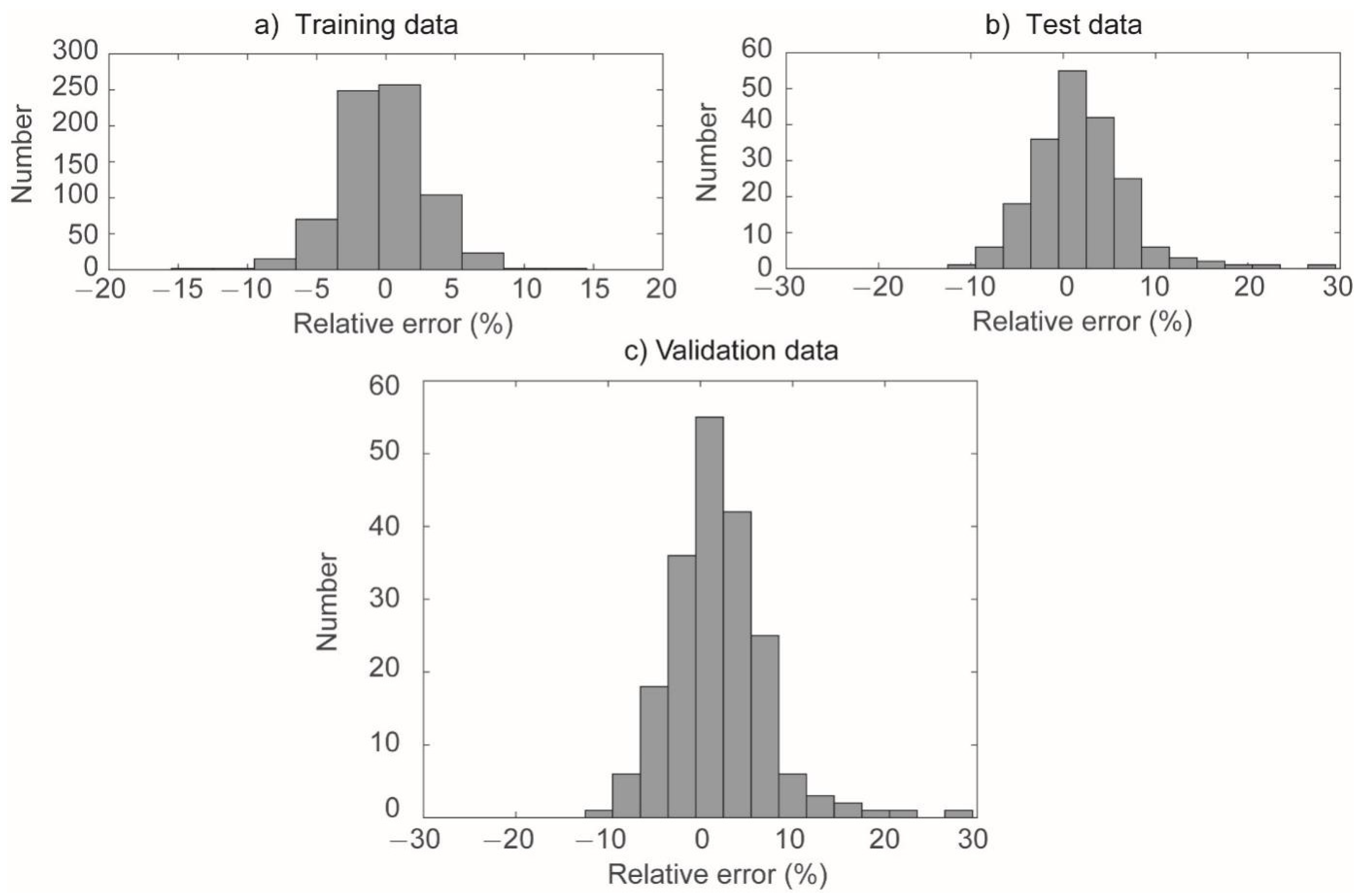
Figure 5.
Flow curves obtained experimentally and applying ANN for training.
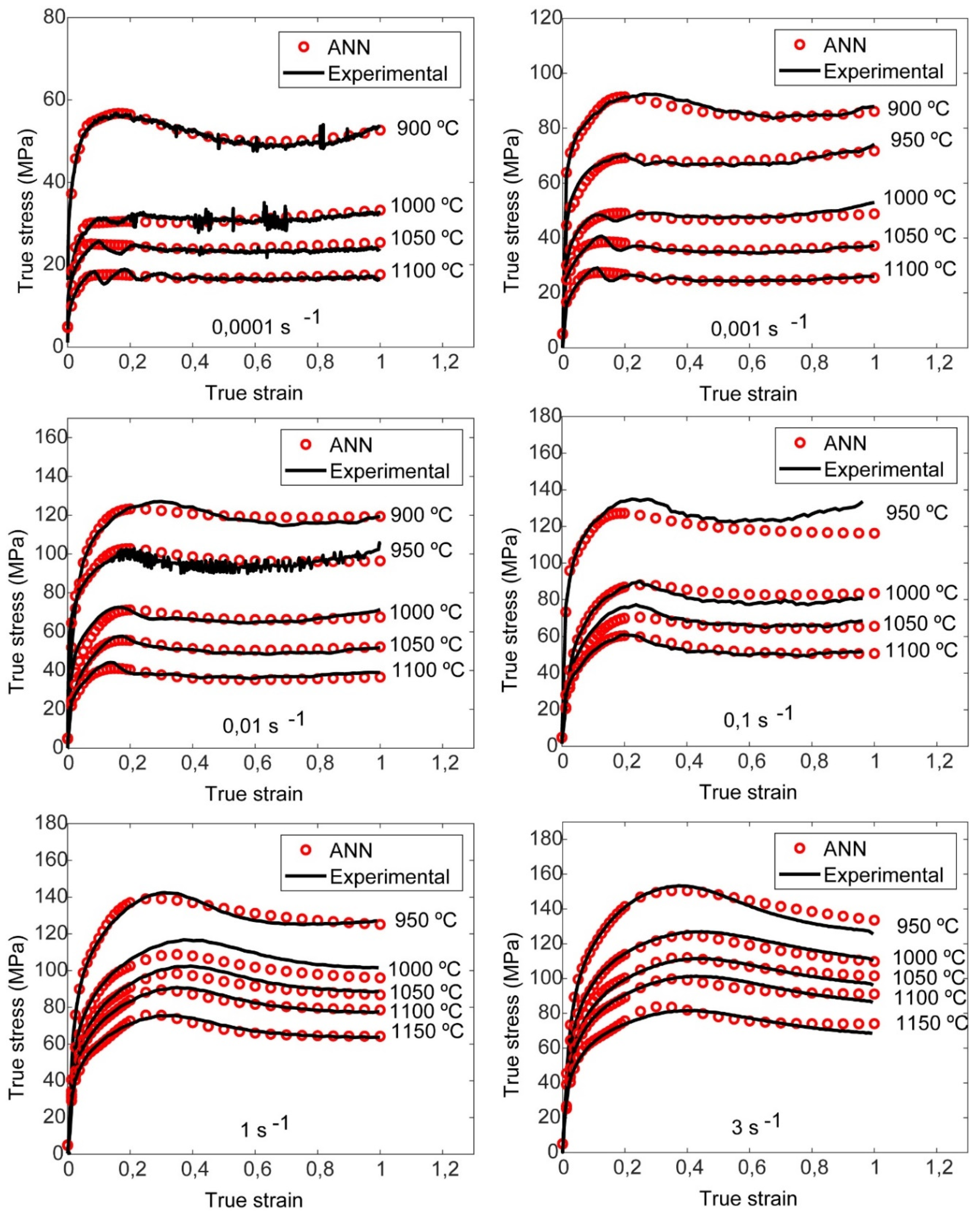
Figure 6.
Flow curves obtained experimentally and applying ANN for training.
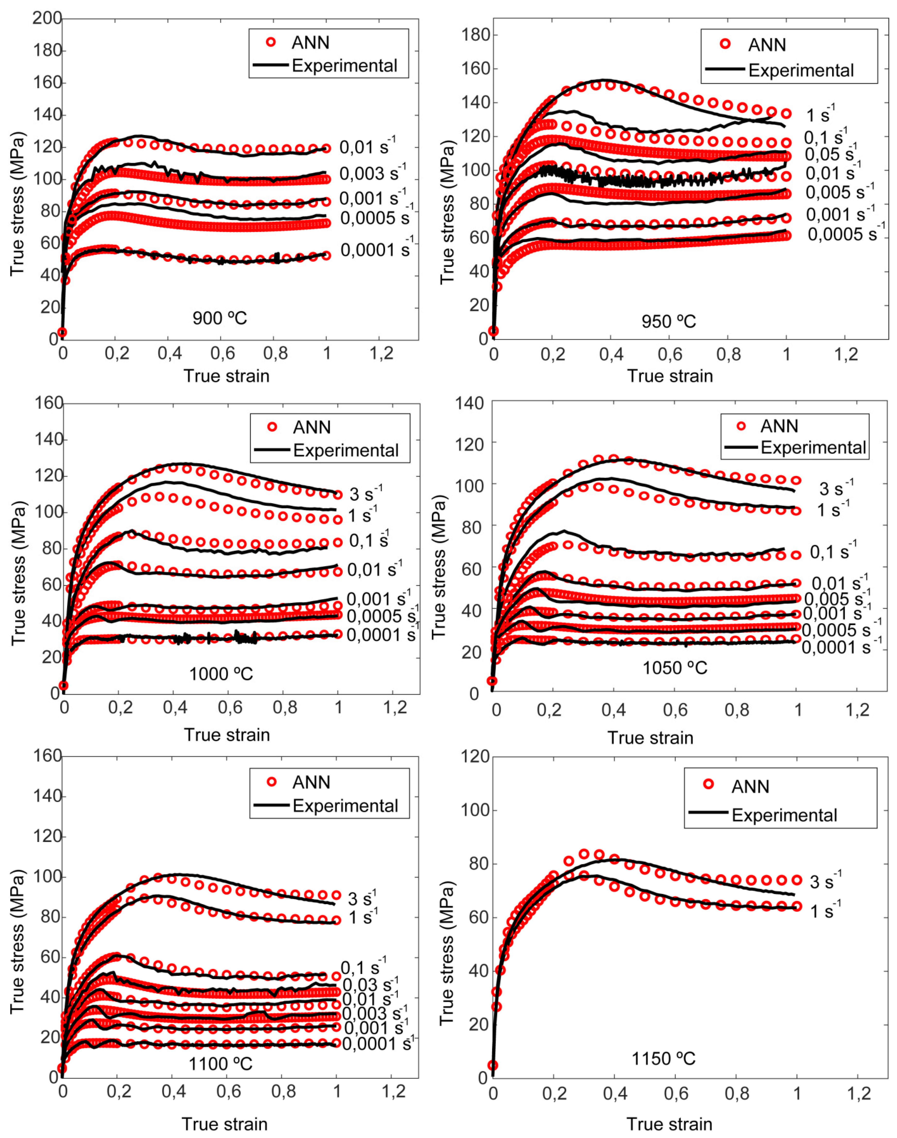
Figure 7.
Flow curves obtained experimentally and applying ANN for the test.
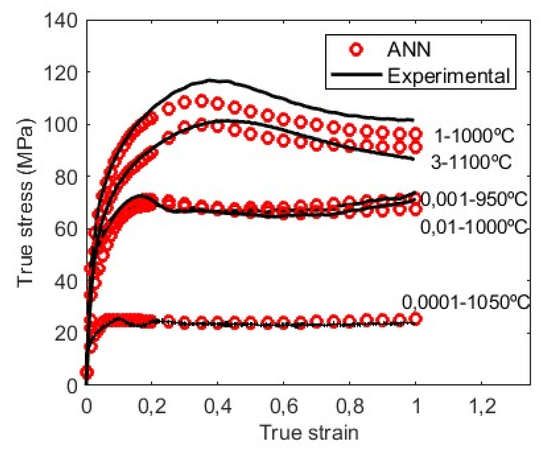
Figure 8.
Flow curves obtained experimentally and applying ANN for validation.
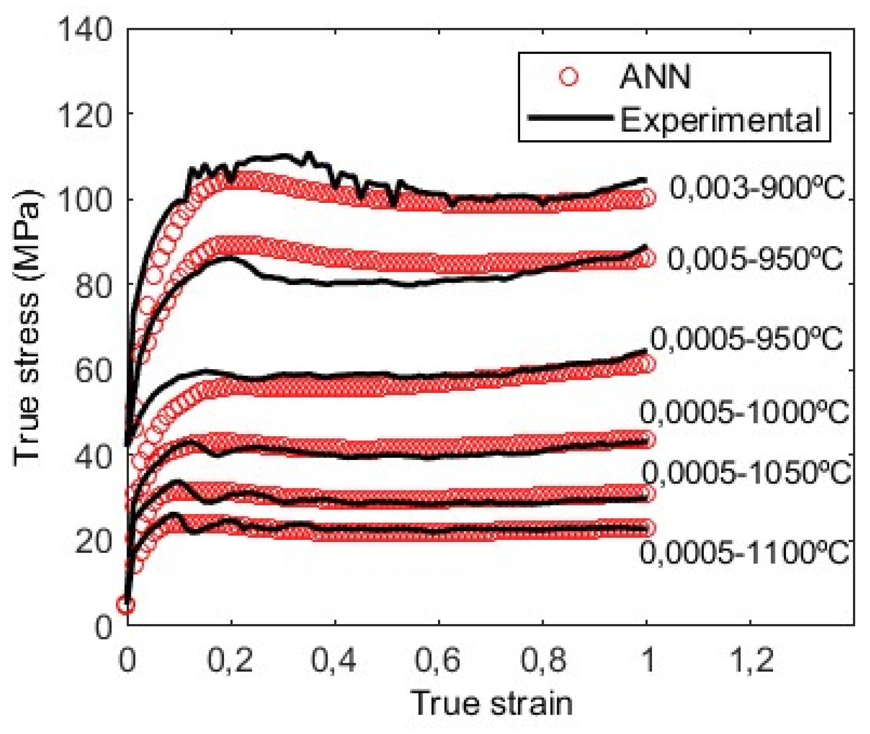
Figure 9.
Experimental processing maps using the VDMM: a) Isoefficiency map b) Plastic instability map.
Figure 9.
Experimental processing maps using the VDMM: a) Isoefficiency map b) Plastic instability map.
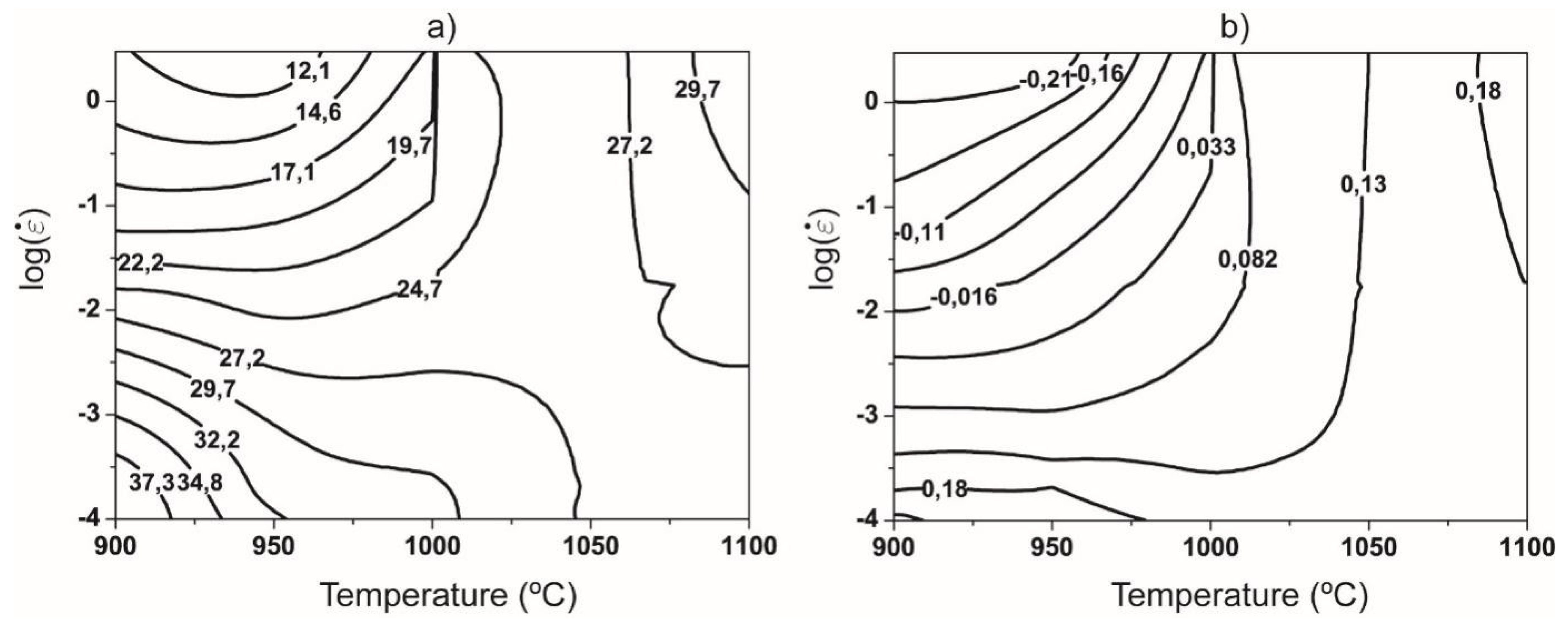
Figure 10.
Processing maps obtained through ANN and based on the DMM for Ɛ=0.6: a) Isoefficiency map b) Plastic instability map.
Figure 10.
Processing maps obtained through ANN and based on the DMM for Ɛ=0.6: a) Isoefficiency map b) Plastic instability map.
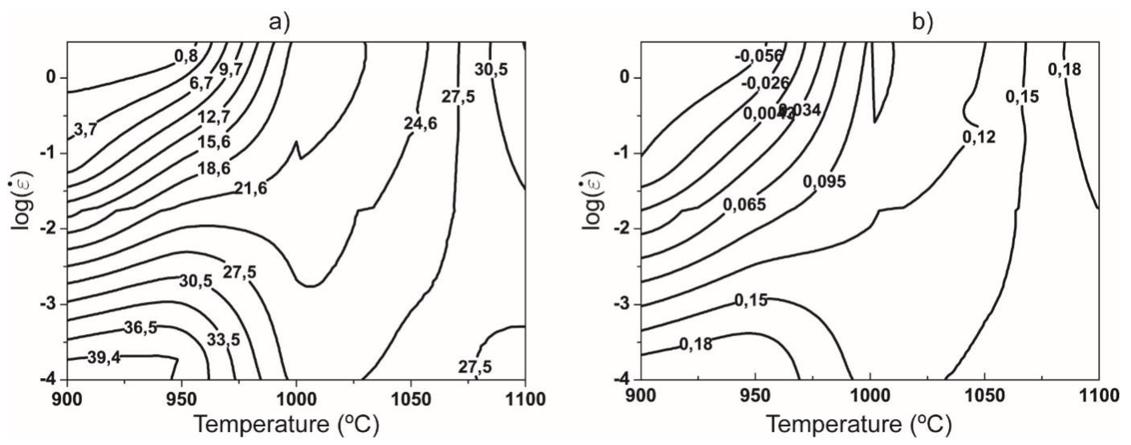
Figure 11.
Processing maps obtained through ANN and based on the VDMM: for Ɛ=0.6: c) Isoefficiency map d) Plastic instability map.
Figure 11.
Processing maps obtained through ANN and based on the VDMM: for Ɛ=0.6: c) Isoefficiency map d) Plastic instability map.
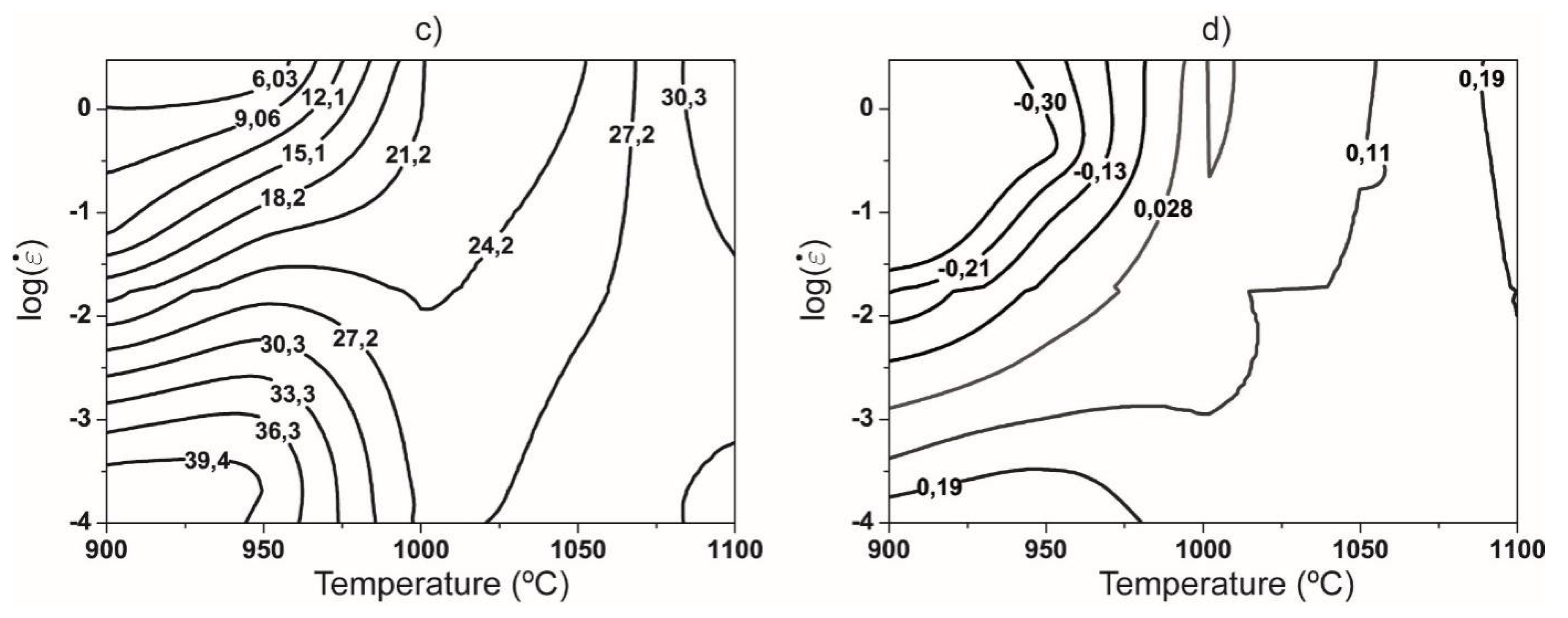
Figure 12.
ANN to obtain the final grain size For the construction of this ANN, 33 experimental data are available for the training, we used 28 (84,8%), and for the test 5 (15,2%). The best results are obtained for a least square error (MSE) of 0,000005. Training stops after 807 iterations.
Figure 12.
ANN to obtain the final grain size For the construction of this ANN, 33 experimental data are available for the training, we used 28 (84,8%), and for the test 5 (15,2%). The best results are obtained for a least square error (MSE) of 0,000005. Training stops after 807 iterations.
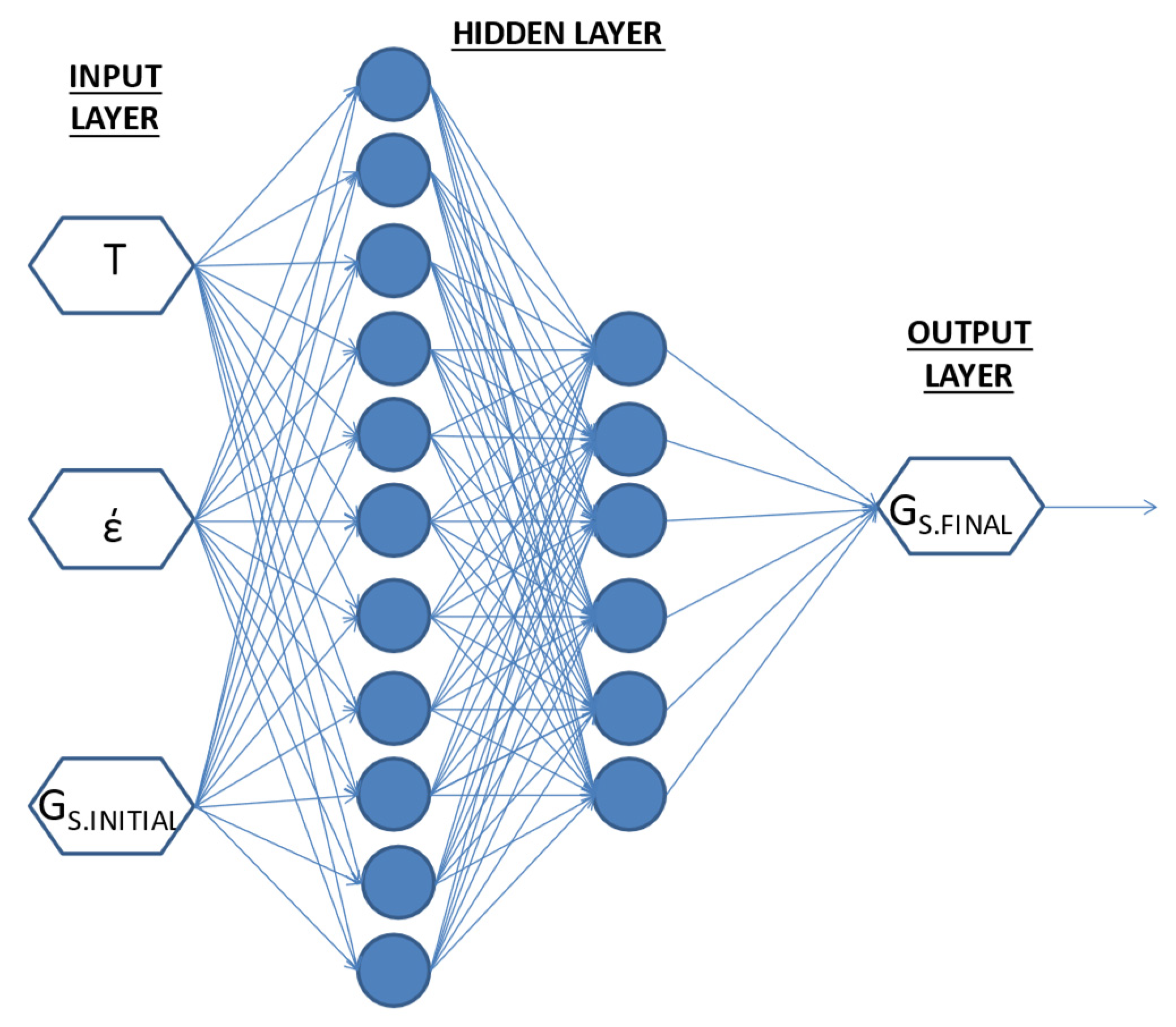
Figure 13.
Evolution of recrystallized grain size for different strain rates.
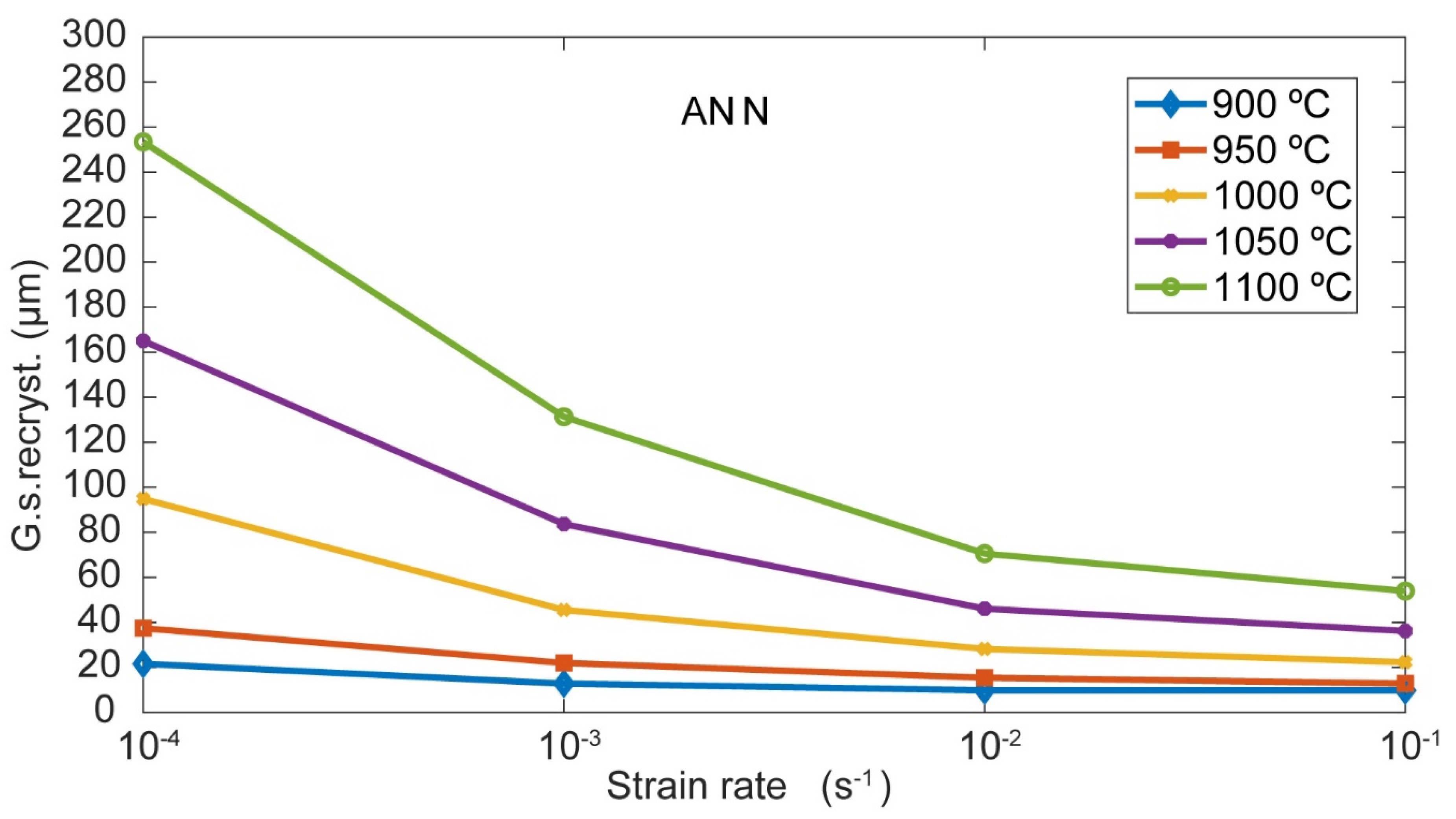
Figure 14.
Evolution of recrystallized grain size for different temperatures and deformation rates.
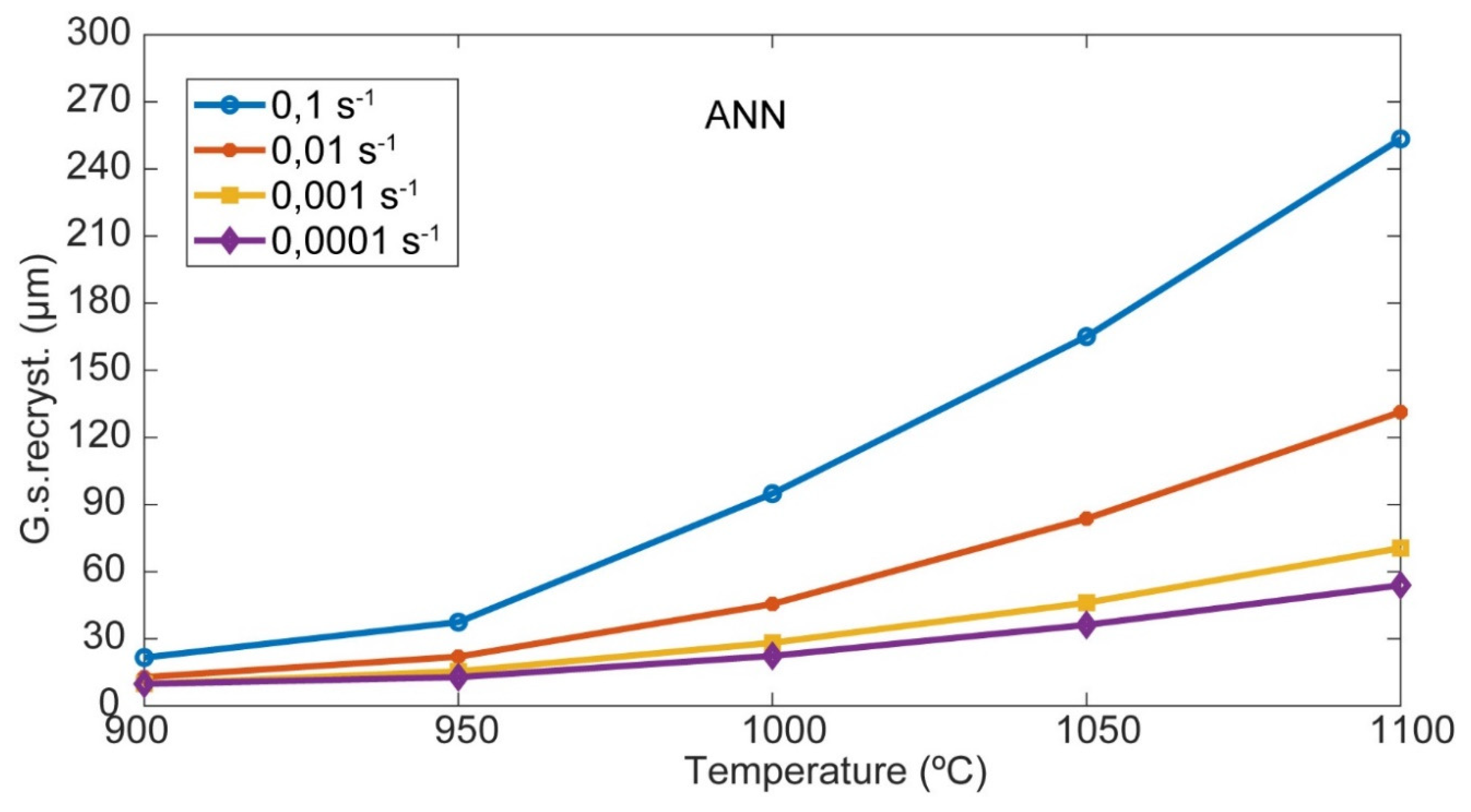
Figure 15.
Final deformed microstructure of M30 Steel at 0.3 s-1 1100ºC.
Disclaimer/Publisher’s Note: The statements, opinions and data contained in all publications are solely those of the individual author(s) and contributor(s) and not of MDPI and/or the editor(s). MDPI and/or the editor(s) disclaim responsibility for any injury to people or property resulting from any ideas, methods, instructions or products referred to in the content. |
© 2024 by the authors. Licensee MDPI, Basel, Switzerland. This article is an open access article distributed under the terms and conditions of the Creative Commons Attribution (CC BY) license (http://creativecommons.org/licenses/by/4.0/).
Copyright: This open access article is published under a Creative Commons CC BY 4.0 license, which permit the free download, distribution, and reuse, provided that the author and preprint are cited in any reuse.