
Submitted:
17 January 2024
Posted:
18 January 2024
You are already at the latest version
Abstract
Explosive boiling is a fast phase transition from an ultra-thin liquid film to vapor under an extremely high heat flux, which typically has been studied using molecular dynamics simulation (MDS) method. The present MDS study investigated the explosive boiling of a liquid argon nanofilm over different solid copper surfaces with different nanowall patterns including parallel and cross nanowalls. For each surface, atomic motion trajectories, number of liquid and vapor argon atoms, heat flux, and, mainly, onset time of explosive boiling were investigated. The simulation results indicated that explosive boiling occurs earlier on parallel and cross nanowall surfaces than on an ideally smooth surface, regardless of the topology and configuration of nanowalls. Moreover, the results revealed that by using the cross nanowall surfaces, the onset time of explosive boiling decreased by 0.7–4% compared to the parallel nanowall surfaces. In addition, it was found that the onset time of explosive boiling strongly depends on the potential energy barrier and the movement space between nanowalls for both parallel and cross nanowall surfaces. Furthermore, simulation findings showed that even though increasing the height of cross nanowalls increases heat flux and temperature of the fluid argon domain, it does not necessarily result in a shorter onset time of explosive boiling. These findings demonstrate the capability of cross nanowall surfaces for explosive boiling, thereby could be utilized in future surface design for thermal management applications.
Keywords:
Explosive boiling
; Molecular dynamics simulations
; Liquid nanofilm
; Nanostructurned surface
; Onset time
1. Introduction
Studying the phase transition phenomena of ultra-thin liquid films on a solid surface is important for science and practical applications. Based on the surface temperature, phase transitions can occur in a normal or explosive boiling mode [1]. During explosive boiling, the liquid is heated considerably more than its saturation temperature but lower than its critical temperature by laser heating or sudden immersion in a hot medium, so a sharp pressure increase accompanies the phase transition, which leads to the liquid being ejected from the surface in a very short time. Therefore, explosive boiling is extremely violent and rapid, resembling an explosion [2,3].
Due to the miniaturization of microelectronic devices, heat dissipation has become a serious problem, which limits the development of some technologies, such as laser surgery and ink-jet technology [4,5]. In this scenario, explosive boiling could represent a powerful method to advance the heat transfer efficiency of hot surfaces. Consequently, improving our understanding of this phenomenon is a compelling and vital topic to increase the thermal energy conversion efficiency of new technologies.
Experiments at a large scale have shown that surface roughness, including the topology (shape) and configuration (size) of nanostructures, significantly impacts explosive boiling heat transfer. Even though almost all solid surfaces exhibit some molecular-level roughness, it is possible to design unique nanopatterns on a flat surface with the evolution of nano-manipulating technology [6]. Subsequently, great possibilities to pursue more efficient nanostructured surfaces for explosive boiling heat transfer have recently drawn significant attention.
Although explosive boiling of ultra-thin liquid films has been experimentally investigated in recent years [7,8], a profound comprehension of physical phenomena based on macroscopic experiments is not fully understood owing to the intricacy of physical phenomena at the nanoscale, the limits on the time scale, and extremely high heat fluxes and temperatures [3]. Therefore, this phenomenon remains one of the least understood nanoscale heat transfer topics. With the advancement of computer hardware and software, it has become feasible to investigate transport phenomena on the nanoscale via numerical simulation. In this regard, the molecular dynamics simulations (MDS) method, which can describe any physical process at the atomic level and on a picosecond (ps) time scale, has shown promise as a powerful method for exploring the behavior of explosive boiling on nanostructured surfaces and has been successfully and widely used in recent years.
Since Morshed et al. [1] analyzed explosive boiling of liquid argon nanofilms over platinum surfaces with separated cylindrical nanopillars using the MDS method for the first time, many MDS studies have been carried out to apply different nanostructured surfaces for explosive boiling, which are summarized and tabulated in Table 1. Up until now, the effects of many nanostructure topologies on explosive boiling performance have been investigated via the MDS method. The results have shown that using nanostructured surfaces with various topologies could increase the heat flux [9,10,11,12,13], the onset temperature of explosive boiling [1,3,6,11,12,13,14,15,16,17], the evaporation rate [1,6,9,14,15], the moving velocity of the liquid cluster [1,6,9,10,11,14,15,16,17,18], and reduce the onset time of explosive boiling [1,6,9,10,11,12,13,14,15,16,17,18]. Therefore, the MDS studies proved that nanostructured surfaces could drastically enhance explosive boiling performance. However, they have focused only on either separated nanopillars or parallel nanowalls without considering the influence of connected ones. Using connected nanostructures could alter the absorption of heat flux by the liquid nanofilm. Hence, they should also be of interest from a commercial and scientific viewpoint.
To the best of the authors’ knowledge, the effect of cross nanowall surfaces on explosive boiling has not been investigated within the available literature and remains to be unveiled. Motivated by this kind of nanostructured surface, the main novelty of this study is the investigation of the effect of cross nanowalls, together with parallel nanowalls, on the explosive boiling behavior of liquid nanofilm using the MDS method. Meanwhile, the influences of spacing and height of cross nanowalls on the onset time of explosive boiling are evaluated in the simulations.
This study is structured as follows: initially, the simulation method is explained. After that, the validation of the molecular model is presented. Then, the roles of surface topology and spacing for both parallel and cross nanowall surfaces on the onset time of explosive boiling are investigated. Then, further evaluation of the effect of the height of cross nanowalls is discussed. Finally, the paper is completed with conclusions.
2. Simulation Method and Details
2.1. Simulation Details
Several cases with distinct surface topologies and configurations were studied to examine the impact of cross nanowalls on explosive boiling. The simulation procedure consisted of three steps: Step I: model development; Step II: computational runs; and Step III: post-processing analysis. The details of these steps, which are presented here, were similar for all but two simulation cases. Simulation details for exceptions, simulation Cases I and II, are presented in Section 3.1.1 and Section 3.1.2, respectively.
Even though the simulation procedure may be used for any material combination, argon (Ar) and copper (Cu) were chosen because of the accessibility and convenience of their potential functions [21]. Gravity was ignored in all simulations because it is significantly less meaningful than surface stress for a liquid nanofilm [22]. Using the Velocity-Verlet integration, numerical solving of the classical Newton’s equation of motion was performed. Several papers dealing with the MDS method present the algorithm for solving atom motions (for example, see Refs. [23,24]). All simulations were carried out using the open-source MDS code LAMMPS (large-scale atomic/molecular massively parallel simulator) package [25]. Due to the lack of visualization, the Open Visualization Tool (OVITO) was used for the post-processing analysis [26].
2.2. Model Development
2.2.1. Force Field and Parameters
The most crucial step in the MDS method is selecting a suitable intermolecular potential that characterizes the interaction between atoms and the movement of each atom. Since the present study focuses on the boiling of a liquid argon nanofilm on a solid copper surface, the interactions between them were modeled only by Van der Waals interactions, which have been widely used in several studies dealing with MDS of argon explosive boiling on metal surfaces (for example, see Refs. [1,6,15,17,27]) and have been demonstrated to be reliable. Consequently, the most frequent and well-known formulation of the Lennard-Jones 12-6 (L-J 12-6) function potential (Uij) was applied to characterize the Cu-Cu, Ar-Ar, and Ar-Cu atomic interactions as follows [28]:
where rij denotes the distance between interacting atoms (i and j), and εij and σij represent the energy parameter (the depth of the potential well (eV)) and the length parameter (the specified distance at which the interatomic potential is zero (Å)), respectively. Table 2 lists the energy and length parameters between Ar atoms (Ar-Ar) and Cu atoms (Cu-Cu) obtained from Ref. [9]. However, εAr-Cu and σAr-Cu were determined in the way described below. The Lorentz combination rule (an arithmetic mean) was used to estimate the length parameter between Ar and Cu atoms [29]:
For the energy parameter between Ar and Cu atoms (εAr-Cu), a modified version of the Berthelot rule (a geometric mean) proposed by Din and Michaelides [30] was adopted:
where “α” is the potential energy factor that could be applied to modify the wettability of the solid surface. In the present work, relay to the results by Ref. [20], only the moderate hydrophilic (α=0.14) was considered. It is essential to point out that the word hydrophilicity refers to the wettability phenomena that occur when the liquid is water. If the liquid is other than water, this property should be referred to as lypophilicity. Nonetheless, "hydro" is frequently employed as a generic term regardless of the liquid [31].
Calculating the potential energy is the most time-consuming part of any MDS. When the distance between two atoms exceeds the cut-off radius, there is no interaction between the atoms; consequently, atoms with distances larger than the cut-off radius are eliminated from the energy computation. In order to guarantee the calculation's precision and accelerate the simulations, the cut-off radius was adjusted to 9 Å (see Section A of the Supplementary Material).
In order to maintain the position of Cu atoms throughout the simulations, an individual spring force was applied to each atom; hence, the Cu atoms could vibrate around their initial lattice position. A force of magnitude -Kr (eV/Å) was used at every single step, where K (eV/Å2) is the spring constant and r is the distance between the atom's current location and its original location. In order to obtain an accurate copper surface, it is essential to utilize a realistic spring constant. The spring constant is closely related to Young’s Modules; therefore, it is possible to estimate it as [32]:
where E is Young’s Modules (128.2 GPa at 300 K [33]), and d is its corresponding lattice constant (3.6147 Å) of copper. The above data and correlation give the following value for the spring constant: K= 2.8926 eV/Å2.
2.2.2. Simulation Boxes
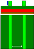
As presented in Figure 1, all simulation cases in this work employed a rectangular simulation cell consisting of three different regions: a solid copper surface (with different topologies and configurations), a liquid argon region, and a vapor argon region. It is important to note that since the number of copper monolayers in different surfaces differed, the height of simulation boxes differed for various simulation cases.
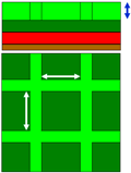
The solid copper surface was created of copper (in face-centered cubic (FCC) with a lattice constant of 3.6147 Å which corresponds to the copper density of 8.93678 g/cm3) and set at the bottom of the simulation boxes so that its 〈0 0 1〉 surface was in touch with the liquid argon region. All the solid copper surfaces had dimensions of 54.2205×54.2205 Å2 in X– and Y– directions. These dimension values were chosen large enough (larger than two times the cut-off radius (9 Å)) to maintain the minimum image convention. In order to better understand the influences of topologies and configurations, various parallel and cross nanowalls with the same dimensions in nanowall width (3.6147 Å) were constructed and simulated. The nanowalls were formed in the upper layer of the ideally smooth surface (the surface F) to create the different nanostructured surfaces. The dimensions of all solid copper surfaces used in this work are tabulated in Table 3, and their related snapshots are shown in Section B of the Supplementary Material (Figure S2). The studied surfaces, termed F, P, and C are ideally smooth and nanostructured surfaces with parallel and cross nanowalls, respectively. The surface ratio was defined as the wetted surface area divided by the nominal surface area at the Ar-Cu interface [34].
As can be seen in Figure S2 and the schematic pictures in Table 3, for all simulation cases, to create a more realistic substrate, the solid copper surface had three different regions from the bottom to the top, namely, the fixed region, the phantom region, and the conduction region. The first monolayer at the bottom of the surface (the fixed region) was kept stagnant to avoid any migration, penetration, and thermal deformation of the solid surface. The next four monolayers (the phantom region), whose temperature was regulated by a thermostat, acted as the heat source for generating heat flux. The remaining monolayers (the conduction region) were set as real atoms from which the liquid argon was heated, thus triggering the explosive boiling process. The nanowall and ideally smooth surfaces are marked with different colors (light and dark green, respectively) to show the topologies and configurations clearly. In the present work, the minimum thickness of copper surfaces (14.4588 Å for the surface F composed of nine monolayers) was still larger than the cut-off radius (9 Å); consequently, the effect of copper thickness can be neglected.
The liquid argon region of the initial thickness of 40.0147 Å, containing 2476 atoms, was placed over the solid copper surfaces. The liquid argon density was 1.3962 g/ml at 87.18 K [35]. These numbers of Ar atoms were adequate to represent actual liquid argon (as will be shown in Section 3.1.1). Moreover, the initial thickness of the liquid argon region was enough to ensure the occurrence of explosive boiling (see Section C in the Supplementary Material).
The space above the liquid argon region was filled by 152 vapor argon atoms (with an initial thickness of 601.7080 Å) with a density of 0.0057 g/ml at 87.18 K [35] to simulate a real phase change system. Considering this, the size of the vapor space in the Z– direction was selected to be large (much greater than the liquid argon nanofilm thickness) so that the top boundary had almost no influence on the explosive boiling process. In addition, the periodic boundary conditions were applied in the X– and Y– directions, so an infinite plane of explosive boiling is simulated, and the non-periodic fixed boundary condition was applied in the Z– direction. This configuration complies with actual experiment procedures [36].
2.3. Computational Runs
The simulation process was divided into four steps: energy minimization, equilibrium preparation, equilibrium relaxation, and non-equilibrium explosive boiling.
Step I (energy minimization): at the beginning of each simulation, after the initial configuration and the interaction force field were prepared, using the conjugate gradient (CG) algorithm, the energy of the whole simulation system was minimized. The stopping tolerances for energy and force were taken as 10-5 eV and 10-5 eV/Å, respectively. Since the potential energy function at the beginning of the next step (Step II) was negligible, the energy minimization method and stopping tolerances were enough to predict the proper atoms' arrangement in space.
Step Ⅱ (equilibrium preparation): in this step, the uniform temperature of the simulation systems was set at 87.18 K, which is the boiling point of liquid argon at 1 bar [35], under the Langevin thermostat for 2000 ps. To avoid entering the liquid Ar atoms in the lattice structure of solid copper surfaces, the liquid Ar atoms were initially located above the solid copper surfaces (during the simulation box construction), and, in this step, they fell onto the surfaces uniformly (see Section D of the Supplementary Material (Figure S4) for the simulation Case P-S2). During this step, all simulation systems reached their equilibrium state. Figure S5 (see Section D of the Supplementary Material) shows a typical fluctuation of temperature and total energy plot for the simulation Case F. It is found that total energy and temperature fluctuations are slight, which satisfies the equilibrium standard. It depicts that the simulation system has reached its equilibrium state.
Step III (equilibrium relaxation): in this step, the simulation systems were run for another 2000 ps while the thermostat was changed into an NVE (i.e., constant atom number, domain volume, and energy) ensemble for the fluid argon domain; however, the temperatures of the solid copper surfaces were still fixed at 87.18 K by the Langevin thermostat. During this period, the temperatures of the Ar and Cu atoms as well as the number of Ar atoms in the liquid and vapor phases were tracked to make sure the system entered a stable condition (see Section E (Figures S6 and S7) of the Supplementary Material for the simulation Case F).
Step IV (non-equilibrium explosive boiling): In this step, the phantom monolayer atoms on solid copper surfaces were heated quickly to 250 K with the Nose-Hoover thermostats to simulate explosive boiling [1], while the rest of the atoms (Ar atoms and Cu atoms in the fixed and conduction monolayers) were free to interact with the NVE ensemble, and simulations were run for 2000 ps. It should be noted that the run time was chosen long enough to cause explosive boiling, and increasing the run time could result in the liquid Ar atoms gradually entering the vapor region, as shown in Section F (Figure S8) of the Supplementary Material for the simulation Case F. The value of 250 K was chosen for the substrate thermostat (the phantom monolayers) to guarantee that explosive boiling occurs.
2.4. Post-Processing Analysis
The trajectories, temperatures, and energies of the atoms in the simulation systems were recorded throughout the simulations, and the desired properties were calculated. The data and snapshot files were exported for post-processing and visualization every 1 ps.
The onset of explosive boiling was defined as the first appearance of a complete layer of vapor film with a thickness of 20 Å over the solid surface. The details are provided in Section G of the Supplementary Material.
For the density studies, the simulation systems were divided into equal bins with a thickness of 2 Å in the direction of the phase change (Z– direction).
Based on the “Oxford” method [37] and definition introduced by Wolde and Frenkel [38], which is remarkably successful in cluster definitions of argon in the MDS method [39], if the distance between two Ar atoms was less than 1.5σAr-Ar (=5.1075 Å), they were considered to be part of the liquid phase. Otherwise, the atoms were considered in the vapor phase. This definition was applied to draw a distinction between the liquid and vapor Ar atoms.
The heat flux between the solid copper surface to the fluid argon domains (liquid and vapor atoms) was calculated by [40]:
here A represents the cross-sectional heat transfer area between solid copper surfaces and Ar atoms, projected onto the X-Y plane (the nominal surface area=54.2205×54.2205 Å2 for all cases in this work), and Ef stands for the total energy of whole Ar atoms (eV). Figure 2 shows the heat flux for the simulation Case F (in units of eV/(Å2 ps) and GW/m2). As can be seen, the heat flux derived in this way (the red lines) is highly fluctuating. Therefore, the results were smoothed out by applying the FFT filter with a filter coefficient equal to 0.4 (see Refs. [4,40] for more details). The blue curves in Figure 2 present the smoothed-out results.
3. Result and Discussion
3.1. Model Validation
In order to determine the reliability of computational accuracies, two different simulation model validations for a liquid argon system (the simulation Case I) and a liquid-vapor argon coexistence system (the simulation Case II) were carried out in this work. Since density is the common evaluation property for validation of the MDS method, this property was calculated and compared with the NIST-data [35], a famous fluid properties database. The methodology, results, and discussion are presented here.
3.1.1. The Simulation Case I: The Liquid Argon System
In this section, to ensure the reliability of the force field to reproduce the structural properties of the liquid argon, a liquid argon box with a dimension equal to 40.0002×40.0002×40.0002 Å3 (consisting of 1360 Ar atoms) was subjected to a 2500 ps simulation under an NPT (isothermal-isobaric) ensemble at 1 bar and 85 K. Notably, the NPT ensemble was used because the simulation box should be allowed to vary in size in order to obtain a well-density equilibrated system. Since the temperature and the total energy are key factors determining the equilibrium state, Figure S11 (see Section H of the Supplementary Material) shows the fluctuation of temperature and total energy for the simulation Case I during the NPT simulation, which are found to be slight, which satisfies the equilibrium standard, and depict that the simulation box has reached its equilibration state. Moreover, Figure 3 shows the change in density and cell length.
3.1.2. The Simulation Case II: The Liquid-Vapor Argon Coexistence System
With the density bouncing constantly around the final stable value of 1.3829 g/ml, which agrees well with the experimental data (1.4096 g/ml [35]), the plot demonstrates that the system is in a stable condition. Moreover, the radial distribution function (RDF) predicted by the molecular simulation is compared with experimental data, as shown in Figure 4. The experimental data were obtained from J. L. Yamell et al. [41], measured in neutron scattering experiments at 85 K. As can be seen, the MDS result matches excellently with the experimental measurement, and the three curves are practically indistinguishable, especially for the second and third peaks. However, for the first peak, the MDS somewhat slightly underestimated the value. This is somewhat expected since the experimental RDF has been measured with an atomic density of 0.02125 atom/Å3 [41], but the average atomic density for the simulation was 0.02085 atom/Å3. This is reasonable because the particles neighboring each other are closer when the density increases. This leads to a higher value for the first peak in experimental data. This is also compatible with the assertion that the force field underestimated liquid density (see Figure 3). Generally, there is reasonably good agreement between the MDS results and the experimental data.
3.1.3. The Simulation Case II: The Liquid-Vapor Argon Coexistence System
A liquid-vapor argon coexistence system (the simulation Case II), as shown in Figure 5, was developed to validate the simulation model for two-phase equilibrium. The liquid film size was 39.9995×39.9995× 39.9995 Å3 (consisting of 1347 Ar atoms) with a 39.9995×39.9995×400.0579 Å3 long vapor domain (consisting of 55 Ar atoms) on each side. During 2500 ps equilibration at 87.18 K (the boiling point of argon at 1 bar [35]) under an NVT ensemble, it is found that total energy and temperature fluctuations are slight, which satisfies the equilibrium standard (Figure S12).
Figure 6 demonstrates a good agreement between the liquid and vapor densities from the simulation and the experimental data. In order to extract the mean value of density distributions along the Z– direction, the system was divided into 210 bins with a height of 4 Å.
Moreover, snapshots from the simulations after 2000, 2250, and 2500 ps are presented in Figure 7. As can be seen, the boundary between the liquid and vapor phases is almost constant. Even though escaping and reentering atoms into the liquid phase could change the surface density, it is not very significant.
Furthermore, as shown in the Supplementary Material (video S1), during the simulation, liquid Ar atoms are evaporating from the liquid surface. However, they are reentering the liquid just as fast as they are escaping from it, which provides a molecular viewpoint on the two-phase equilibrium.
3.2. Simulation Cases A: Effects of Surface Topology and Spacing
Figure 8 illustrates the onset time of explosive boiling for liquid argon nanofilms on solid copper surfaces with different topologies and spacing. The full snapshots are illustrated in Figure S13 (see Section I of the Supplementary Material) for better inspection.
Three main findings can be summarized:
Finding #1: The onset time of explosive boiling of the liquid argon nanofilm over the ideally smooth surface (the simulation Case F) is 538 ps, longer than the nanostructured surfaces (354-513 ps).
Finding #2: For the parallel nanowall surfaces with different spacing (the simulation Cases P-S), the onset time of explosive boiling decreases from 513 ps (for the simulation Case P-S1) to 370 ps (for the simulation Case P-S4) and then increases to 434 ps (for the simulation Case P-S6). The same trend can be seen for the cross nanowall surfaces (the simulation Cases C-S).
Finding #3: The cross nanowall surfaces show a shorter onset time of explosive boiling than the parallel nanowall surfaces.
As mentioned in Finding #1, adding nanowalls could shift the explosive boiling occurrence earlier. The presence of nanowalls increases the contact area between the liquid argon nanofilms and the solid copper surface. Therefore, more liquid Ar atoms will be at the solid-liquid interface, which in turn excels in heat transfer from the solid surface to the fluid argon domain, thereby decreasing the onset time of explosive boiling. To better demonstrate the effect of nanostructured surfaces on the onset of explosive boiling, quantitative analysis of heat flux, the temperature of Ar atoms, and the number of liquid and vapor Ar atoms will be discussed in detail at the end of this section.
Herein, it is presumptive that the effects of the potential energy barrier and the movement space for liquid Ar atoms are what led to Findings #2 and #3. In the following, to investigate the effect of these factors on the onset time of explosive boiling, the parallel nanowall surfaces are chosen (due to more explicit view pictures and easy observation), and the mechanism of explosive boiling from the molecular point of view is discussed. The discussion could be extended to cross nanowall surfaces.
Figure 9 and Figure S14 show the heat flux of the fluid argon domain over parallel nanochannel surfaces with different spacing in eV/(Å2 ps) and GW/m2, respectively. As can be seen, as the solid temperature grew continuously under the thermostat, the heat fluxes reached their maximum. Then they decreased to a relatively low value. The transition from the solid-liquid interface to the solid-vapor interface occurs during this time, which leads to significantly high interfacial thermal resistance (the Kapitza thermal resistance) and consequently lower heat flux. Finally, heat fluxes reach almost zero after the departure of the liquid argon cluster and its vapor-liquid tail from the surface.
Considering the maximum heat flux as the characteristic heat flux [42], Figure 9 also shows that with decreasing nanochannel spacing, the heat flux increases first from 3.406×10⁻⁵ eV/Å2ps (for the simulation Case P-S1) to 9.167×10⁻⁵ eV/Å2ps (for the simulation Case P-S4) and then decreases to 7.080×10⁻⁵ eV/Å2ps (for the simulation Case P-S6). It can be explained by the effect of the potential energy interaction between liquid Ar atoms and Cu atoms on heat transfer. Therefore, in Figure 10, distributions of the potential energies per Ar atom (calculated by Eq. (1)) for different parallel nanowall surfaces are shown. It can be seen from Figure 10 that the potential energy is most concentrated close to the surface of the copper, especially near the nanowalls. Consequently, using nanowalls enhances the interaction of potential energy between the atoms of liquid Ar and the atoms of the copper surface. Thus, it features a significant thermal vibrational coupling, which leads to greater heat flux and an earlier onset time of explosive boiling. However, interestingly, more reduction in the space between nanowalls, and consequently more increase in the interaction potential energy, resulted in lower heat fluxes for the simulation Cases P-S5 and P-S6. Therefore, the onset time of explosive boiling cannot be determined solely by the value of the interaction potential energy, and there must be other reasons. Herein, this unexpected behavior is attributed to the space for the motion of Ar atoms (movement space). Therefore, for further analysis, the motion of Ar atoms should be studied via their line trajectories.
Figure 11 indicates the snapshots of the line trajectories of 31 randomly selected liquid Ar atoms between the nanowalls for the simulation Cases P-S4, P-S5, and P-S6. Inspection of Figure 11 manifests more spacing reduction beyond the simulation Case P-S4, not only resulting in a significant decrease in the number of Ar atoms between the nanowalls but also a clear reduction of their mobility. In other words, the movement of Ar atoms in the larger space (the simulation Case P-S4) is much better than the smaller ones (the simulation Cases P-S5 and P-S6). Therefore, other than the interaction potential energy, the effect of the movement space on the onset of explosive boiling is significant. When the solid-liquid interactions are very large and, on the other hand, the movement space is very small, the liquid Ar atoms cannot move freely. The lower the movement of liquid atoms, the less they collide, so heat transfer occurs at a lower flux (as previously shown in Figure 9). Furthermore, a small spacing could hinder the constant presence of liquid Ar atoms between the nanowalls. In other words, the small spacing between nanowalls could stop the Ar atoms from re-penetrating into the nanochannels, decreasing the heat flux between the liquid nanofilm and the solid surface. Moreover, breaking the high potential energy barrier takes more time, which accounts for the relatively long time required for the onset of explosive boiling. Therefore, the onset of explosive boiling is delayed.
In general, increasing the surface ratio (i.e., decreasing the channel spacing) can improve explosive boiling performance as a result of an increase in interaction potential energy. However, when the channel spacing is below a critical threshold, an increase in the surface ratio will decrease heat transfer. Regardless of the topology (either parallel or cross nanowall surfaces), the impact of the potential energy barrier and the movement space are always present. Therefore, similar results and discussion could be provided for cross nanowall surfaces (the simulation Cases C-S): the reduction of spacing has an initial promoting effect, but as it passes the critical threshold, it has a negative effect on the starting point of explosive boiling.
This discussion can also define the shorter onset time for cross nanowall surfaces (Finding #3). Cross nanowall surfaces with almost the same surface ratio as parallel ones could provide more movement space for Ar atoms. For example, even though the simulation Cases P-S4 and C-S2 have an almost equal surface ratio (2.3333 and 2.2445, respectively), the spacing length for the simulation Case C-S2 is 23.4956 Å almost two times that of the simulation Case P-S4 (9.0368 Å). Thus, liquid Ar atoms could escape faster from the cross nanowall surfaces than the parallel ones. Consequently, they could better promote explosive boiling and reduce its onset time.
To better compare heat transfer characteristics for different surface topologies, the ideally smooth surface (the simulation Case F) and two nanostructured surfaces with almost equal surface ratios (the simulation Cases P-S4 and C-S2) are selected and discussed in the following.
The heat fluxes for the simulation Cases F, P-S4, and C-S2 in eV/(Å2ps) and GW/m2 are presented in Figure 12 and Figure S15, respectively. It is seen that due to the presence of nanowalls, the solid-liquid interface area and interaction between the solid copper and liquid argon atoms increase, resulting in a substantial difference between the heat fluxes of the ideally smooth surface (the simulation Case F) and nanostructured surfaces (the simulation Cases P-S4 and C-S2). In addition, the heat flux on surfaces with cross nanowalls is greater than that on surfaces with parallel nanowalls.
The simulation results of the temperature history of Ar atoms are shown in Figure 13. The Ar temperature represents the temperature of all argon atoms, including liquid and vapor atoms. The plot is limited to 600 ps to have a clear view of the onset time of explosive boiling. For the simulation cases with parallel and cross nanowalls (the simulation Cases P-S4 and C-S2, respectively), Ar atoms get more heated than the ideally smooth surface (the simulation Case F), as described in the last section. Moreover, with the presence of nanostructures, the distance from the solid surface to the top liquid argon layer decreases. As a result, the temperature of the liquid Ar atom on the nanostructured surface is higher than on the ideally smooth surface. Even though for the simulation Case P-S4 and C-S2, the average conduction path of the liquid layers is practically identical, the simulation Case C-S2 shows a slightly higher argon temperature because of its slightly higher heat flux (see Figure 12).
The quantity of liquid and vapor atoms in the system during the non-equilibrium explosive boiling is depicted in Figure 14. It is important to keep in mind that the variation in the quantity of vapor atoms reflects the system's rate of evaporation. For all simulation cases, the number of liquid Ar atoms decreases after the beginning of boiling. However, the number of liquid argon atoms decreases earlier for the simulation Cases C-S2 and P-S4, followed by the simulation Case F, which implies that the evaporation rate is higher for nanostructured surfaces. In other words, the greater heating area and heat flux on nanostructured surfaces cause highly rapid liquid evaporation at the start of boiling, quickly changing the liquid-to-vapor ratio in the system.
Furthermore, the results indicate that even though the evaporation ratios of surfaces with nanostructures are nearly comparable, the simulation Case C-S2 is slightly higher than that of the simulation Case P-S4 due to the larger space for moving Ar atoms and, consequently, a higher heat flux, as described before. It is interesting for all simulation cases that the liquid cluster before the detachment absorbs high values of heat flux from the heated substrate. Therefore, the liquid argon clusters still maintain a high evaporation rate even after detachment.
The study of the density profiles is important because it indicates the density and velocity of the liquid argon cluster. Figure 15 shows the density profile of the fluid argon domain in the Z- direction for simulation Cases F, P-S4, and C-S2 at various times.
Three distinct zones can be seen in the density profiles. With a relatively high density, the liquid phase forms the first region, the liquid-vapor interface forms the second, and the vapor phase forms the third. Because there are a few atoms in the vapor region, the local density in this area exhibits some scattering. The peak values of the density profile at the onset time of explosive boiling for the simulation Cases F, P-S4, and C-S2 are 2.6605, 2.6113, and 2.5397 mol/l, respectively. This means that using the cross nanowall surface leads to a floating liquid argon cluster with a lower density, compared that the ideally smooth and the parallel nanowall surfaces. It relies mainly on the fact that the cross nanowall surface could increase the Ar temperature higher than the others (Figure 13). Moreover, because of a low-density floating liquid argon cluster for the simulation Case C-S2, its upward velocity is higher.
For a better visual demonstration of explosive boiling on different surface topologies, video S2, S3, and S4, are provided for the simulation Cases F, P-S4, and P-S2, respectively.
3.3. Simulation Cases B: Effects of Nanowall Height
In this section, aiming to understand the effect of the height of nanowalls on the onset time of explosive boiling, the nanowall height for cross nanowall surfaces was changed, whereas the spacing was kept fixed. Three different heights (3.6147 Å (the simulation Case C-H1), 9.0368 Å (the simulation Case C-H2), and 12.6515 Å (the simulation Case C-H3)) were investigated.
Figure 16 illustrates the onset time of explosive boiling for liquid argon nanofilms over cross nanowall surfaces with different heights. The full snapshots are illustrated in Figure S16 (see Section J of the Supplementary Material) for better inspection.
As shown in Figure 16, the onset time of explosive boiling decreases from 470 ps (for the simulation Case C-H1) to 354 ps (for the simulation Case C-H2) and then increases to 375 ps (for the simulation Case C-H3).
The heat fluxes for the simulation Cases C-H1, C-H2, and C-H3 in eV/(Å2 ps) and GW/m2 are presented in Figure 17 and Figure S17, respectively. It can be seen that the maximum heat flux rises with the increase in nanowall height because the solid–liquid interface area increases. Therefore, increasing the nanowall height means the fluid argon domain could obtain more energy, resulting in a higher argon temperature, as shown in Figure 18. However, interestingly, more increases in the nanowall height resulted in postponing the onset of explosive boiling.
As discussed in the previous section, the interaction potential energy and movement spacing are the key parameters that could determine the onset time of explosive boiling. In this section, the movement spacing was the same (23.4956 Å) for all simulation cases. Considering only the impact of interaction potential energy (illustrated in Figure 19), the lower interaction potential energy for simulation Case C-H1 is the main reason for its lower heat flux and prolonged onset time. Nevertheless, the effect of interaction potential energies for simulation Cases C-H2 and C-H3 is unusual.
The interaction potential energies and heat flux increased as the nanowall height was increased (from 9.0368 for simulation Case C-H2 to 12.6515 for simulation Case C-H3). Nonetheless, it also delays the onset of explosive boiling. Bai et al. [12] showed that increasing the height of the parallel nanowalls increased the heat flux and reduced the onset time of explosive boiling. Thus, the trend of the present work disputes the results in Ref. [12]. However, it can be explained by the difference in wettability. Bai et al. [12] used water and copper as the liquid nanofilm and solid surface, respectively. The energy parameter for water-copper interaction is much larger than that for argon-copper. This significant energy parameter (0.0342 eV) causes the water molecules to stay between the nanowalls during explosive boiling, and the cluster liquid separation starts above the nanowalls. Nevertheless, in this study, explosive boiling starts between the nanowalls because of the lower energy parameter for argon-copper interaction (0.0065 eV). In this situation, when the height of the nanowall is significant compared to the thickness of the liquid nanofilm, increasing the height of the nanowall may have an adverse effect on the onset time. In other words, although more liquid atoms between higher nanowalls could absorb more heat and reach a higher temperature, they could not overcome the incredible interaction potential energy barrier in the direction of the phase change (the Z– direction) and start explosive boiling. As can be seen in Figure 19, compared to simulation Case C-H2, simulation Case C-H3 has a more significant number of Ar atoms with high interaction potential energies (-0.04 – -0.08 eV/atom) between the nanowalls.
4. Conclusions
In this study, using the molecular dynamics simulation method and LAMMPS software, the effect of cross nanowalls on the onset time of explosive boiling of a liquid argon nanofilm on a solid copper substrate was examined. The first part proved the model's validity by analyzing density and radial distribution functions. Then three different topologies were simulated, including an ideally smooth surface, parallel nanowall surfaces, and cross nanowall surfaces. Based on the results, the presence of the cross nanowalls accelerates the onset of explosive boiling. Furthermore, the optimum spacing for the parallel and cross nanochannel surfaces was determined by the analysis of the effect of nanochannel spacing on the onset time of explosive boiling. It is also observed that the potential energy barrier and movement space play a substantial role in the onset time of explosive boiling. At last, the results revealed that the potential energy barrier not only could have an influence on the optimum space between the nanowalls for both parallel and cross nanowall surfaces, but it could also have a significant effect on the optimum height of the nanowall (for the cross nanowall topology) when the explosive boiling starts right on the solid copper surface.
Finally, it should be emphasized that the results presented in this paper were obtained for only a moderate hydrophilic substrate. Therefore, in future studies, the effect of surface wettability should be investigated for a better understanding of explosive boiling on cross nanowall surfaces.
Conflict of Interest Statement
On behalf of all authors, the corresponding author states that there is no conflict of interest.
Supplementary Materials
The following supporting information can be downloaded at the website of this paper posted on Preprints.org.
Nomenclature
| A | Nominal surface area | (Å2) |
| Å | Angstrom | - |
| d | Lattice constant | (Å) |
| E | Young’s Modules | (GPa) |
| Total energy of fluid atoms. | (eV) | |
| FCC | Face-centered-cubic | - |
| GW | Gigawatt | - |
| K | Spring constant | (eV/Å2) |
| L-J 12-6 | Lennard-Jones 12-6 | - |
| m | Meter | - |
| MDS | Molecular dynamics simulations | - |
| NVE | Microcanonical ensemble | - |
| NPT | Isothermal–isobaric ensemble | - |
| NVT | Canonical ensemble | - |
| OVITO | Open Visualization Tool | - |
| ps | Picosecond | - |
| q | Heat flux | (eV/Å2ps) |
| r | Distance between the particles | (Å) |
| RDF | Radial distribution function | - |
| t | Time | (ps) |
| T | Temperature | (K) |
| U | Potential energy | (eV) |
| Greek Symbols | ||
| Potential energy factor | ||
| Energy parameter for L-J 12-6 potential | (eV) | |
| Length parameter for L-J 12-6 potential | (Å) | |
| Subscripts | ||
| Ar | Argon | |
| Cu | Copper | |
| i | Particle i | |
| j | Particle j | |
References
- A.M. Morshed, T. C. Paul, J. A. Khan. Effect of nanostructures on evaporation and explosive boiling of thin liquid films: a molecular dynamics study. Applied Physics A 105 (2011) 445–451. [CrossRef]
- P. Bai, L. Zhou, X. Du. Effects of surface temperature and wettability on explosive boiling of nanoscale water film over copper plate. International Journal of Heat and Mass Transfer 162 (2020) 120375. [CrossRef]
- Y. Mao, Y. Zhang. Molecular dynamics simulation on rapid boiling of water on a hot copper plate. Applied Thermal Engineering 62 (2014) 607–612. [CrossRef]
- M. Ilic, V. D. Stevanovic, S. Milivojevic, M. M. Petrovic. New insights into physics of explosive water boiling derived from molecular dynamics simulations. International Journal of Heat and Mass Transfer 172 (2021) 121141. [CrossRef]
- Y. Tang, Y. He, L. Ma, X. Zhang, J. Xue. Molecular dynamics simulation of carbon nanotube-enhanced laser induced explosive boiling on a free surface of an ultrathin liquid film. International Journal of Heat and Mass Transfer 127 (2018) 237–243. [CrossRef]
- H.R. Seyf, Y. Zhang. Molecular dynamics simulation of normal and explosive boiling on nanostructured surface. ASME Journal of Heat and Mass Transfer 135 (2013) 121503. [CrossRef]
- S. I. Kudryashov, S. D. Allen. Photoacoustic study of explosive boiling of a 2-propanol layer of variable thickness on a KrF excimer laser-heated Si substrate. Journal of Applied Physics 95 (2004) 5820–5827. [CrossRef]
- S. I. Kudryashov, S. D. Allen. Submicron dynamics of water explosive boiling and lift-off from laser-heated silicon surfaces, Journal of Applied Physics 100 (2006) 104908. [CrossRef]
- H. Liu, X. Qin, S. Ahmad, Q. Tong, J. Zhao. Molecular dynamics study about the effects of random surface roughness on nanoscale boiling process. International Journal of Heat and Mass Transfer 145 (2019) 118799. [CrossRef]
- P. Zhang, L. Zhou, L. Jin, H. Zhao, X. Du. Effect of nanostructures on rapid boiling of water films: a comparative study by molecular dynamics simulation. Applied Physics A 125 (2019) 142. [CrossRef]
- J. Zhou, S. Li, S-Z Tang, D. Zhang, H. Tian. Effect of nanostructure on explosive boiling of thin liquid water film on a hot copper surface: a molecular dynamics study. Molecular Simulation 48 (2022) 221-230. [CrossRef]
- P. Bai, L. Zhou, X. Du. Molecular dynamics simulation of the roles of roughness ratio and surface potential energy in explosive boiling. Journal of Molecular Liquids 335 (2021) 116169. [CrossRef]
- P. Bai, L. Zhou, X. Du. Effects of liquid film thickness and surface roughness ratio on rapid boiling of water over copper plates. International Communications in Heat and Mass Transfer 120 (2021) 105036. [CrossRef]
- H.R. Seyf, Y. Zhang. Effect of nanotextured array of conical features on explosive boiling over a flat substrate: A nonequilibrium molecular dynamics study. International Journal of Heat and Mass Transfer 66 (2013) 613–624. [CrossRef]
- W. Wang, H. Zhang, C. Tian, X. Meng. Numerical experiments on evaporation and explosive boiling of ultra-thin liquid argon film on aluminum nanostructure substrate. Nanoscale Research Letters 158 (2015). [CrossRef]
- T. Fu, Y. Mao, Y. Tang, Y. Zhang, W. Yua. Effect of nanostructure on rapid boiling of water on a hot copper plate: a molecular dynamics study. Heat and Mass Transfer 52 (2016) 1469–1478. [CrossRef]
- S. Zhang, F. Hao, H. Chen, W. Yuan, Y. Tang, X. Chen. Molecular dynamics simulation on explosive boiling of liquid argon film on copper nanochannels. Applied Thermal Engineering 113 (2017) 208–214. [CrossRef]
- Qasemian, M. Qanbarian, B. Arab. Molecular dynamics simulation on explosive boiling of thin liquid argon films on cone-shaped Al–Cu-based nanostructures. Journal of Thermal Analysis and Calorimetry 145 (2021) 269–278. [CrossRef]
- M-J Liao, L-Q Duan. Explosive boiling of liquid argon films on flat and nanostructured surfaces. Numerical Heat Transfer, Part A: Applications 78 (2020) 94-105. [CrossRef]
- H. Liu, W. Deng, P. Ding, J. Zhao. Investigation of the effects of surface wettability and surface roughness on nanoscale boiling process using molecular dynamics simulation. Nuclear Engineering and Design 382 (2021) 111400. [CrossRef]
- R. Wang, S. Qian, Z. Zhang. Investigation of the aggregation morphology of nanoparticle on the thermal conductivity of nanofluid by molecular dynamics simulations. International Journal of Heat and Mass Transfer 127 (2018) 1138–1146. [CrossRef]
- Y. Yu, X. Xu, J. Liu, Y. Liu, W. Cai, J. Chen. The study of water wettability on solid surfaces by molecular dynamics simulation. Surface Science 714 (2021) 121916. [CrossRef]
- C. Hu, L. Shi, C. Yi, M. Bai, Y. Li, D. Tang. Mechanism of enhanced phase-change process on structured surface: Evolution of solid-liquid-gas interface. International Journal of Heat and Mass Transfer 205 (2023) 123915. [CrossRef]
- X. Yin, C. Hu, M. Bai, J. Lv. An investigation on the heat transfer characteristics of nanofluids in flow boiling by molecular dynamics simulations. International Journal of Heat and Mass Transfer 162 (2020) 120338. [CrossRef]
- Paula Leite, R. and M. de Koning, Nonequilibrium free-energy calculations of fluids using LAMMPS. Computational Materials Science 159 (2019) 316–326. Available online: https://lammps.sandia.gov. [CrossRef]
- Stukowski. Visualization and analysis of atomistic simulation data with OVIT- the Open Visualization Tool. Modelling and Simulation in Materials Science and Engineering 18 (2010) 015012. Available online: http://ovito.sourceforge.net/. [CrossRef]
- Y. Chen, J. Li, B. Yu, D. Sun, Y. Zou, D. Han. Nanoscale Study of Bubble Nucleation on a Cavity Substrate Using Molecular Dynamics Simulation. Langmuir 34 (2018) 14234−14248. [CrossRef]
- M. Zarringhalam, H. Ahmadi-Danesh-Ashtiani, D. Toghraie, R. Fazaeli. Molecular dynamic simulation to study the effects of roughness elements with cone geometry on the boiling flow inside a microchannel. International Journal of Heat and Mass Transfer 141 (2019) 1–8. [CrossRef]
- J. Delhommelle, P. Millié. Molecular physics: an international journal at the interface between chemistry and physics. Molecular physics 99 (2001) 619–625. [CrossRef]
- X.D. Din, E.E. Michaelides. Kinetic theory and molecular dynamics simulations of microscopic flows. Physics of Fluids 9 (1997) 3915–3925. [CrossRef]
- Hens, R. Agarwal, G. Biswas. Nanoscale study of boiling and evaporation in a liquid Ar film on a Pt heater using molecular dynamics simulation. International Journal of Heat and Mass Transfer 71 (2014) 303–312. [CrossRef]
- Y. Chen, Y. Zou, D. Sun, Y. Wang, B. Yu. Molecular dynamics simulation of bubble nucleation on nanostructure surface. International Journal of Heat and Mass Transfer 118 (2018) 1143–1151. [CrossRef]
- R.P. Reed, A. F. Clark. Materials at low temperatures. American Society for Metals, 1983. [CrossRef]
- H. Hu, Y. Sun. Effect of nanopatterns on Kapitza resistance at a water-gold interface during boiling: A molecular dynamics study. Journal of Applied Physics 112, 053508 (2012). [CrossRef]
- NIST Chemistry WebBook, NIST Standard Reference Database, NIST Chemistry WebBook. [CrossRef]
- Y. Hea, S. Wanga, Y. Tanga, Z. Wub, W. Li. Molecular dynamics simulation on liquid nanofilm boiling over vibrating surface. International Journal of Heat and Mass Transfer 201 (2023) 123617. [CrossRef]
- X. Deng, X. Xu, X. Song, Q. Li, C. Liu. Boiling heat transfer of CO2/lubricant on structured surfaces using molecular dynamics simulations. Applied Thermal Engineering 219 (2023) 119682. [CrossRef]
- P.R. ten Wolde, D. Frenkel. Computer simulation study of gas–liquid nucleation in a Lennard-Jones system. The Journal of Chemical Physics 109 (1998) 9901. [CrossRef]
- J. Wedekinda, D. Reguera. What is the best definition of a liquid cluster at the molecular scale. The Journal of Chemical Physics 127 (2007) 154516. [CrossRef]
- M. Ilic, V. D. Stevanovic, S. Milivojevic, M. M. Petrovic. Explosive boiling of water films based on molecular dynamics simulations: Effects of film thickness and substrate temperature. Applied Thermal Engineering 220 (2023) 119749. [CrossRef]
- J.L. Yarnell, M.J. Katz, R.G. Wenzel, S.H. Koenig. Structure factor and radial distribution function for liquid argon at 85 °K. Physical Review A 7 (1973) 2130–2144. [CrossRef]
- H. Liu, S. Ahmad, J. Chen, J. Zhao. Molecular dynamics study of the nanoscale boiling heat transfer process on nanostructured surfaces. International Journal of Heat and Mass Transfer 191 (2022) 122848. [CrossRef]
Figure 1.
A typical snapshot of the initial configuration of simulation systems.
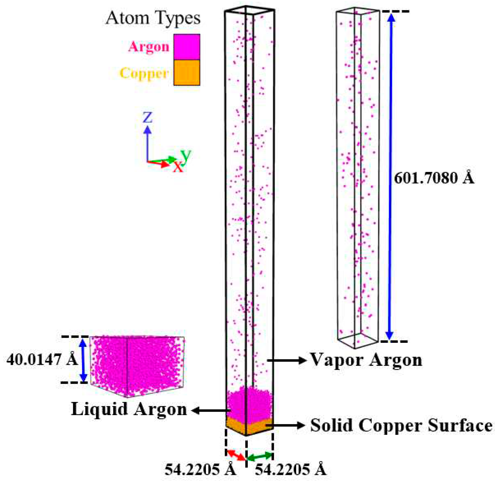
Figure 2.
Unsmoothed and smoothed heat flux for the simulation Case F.
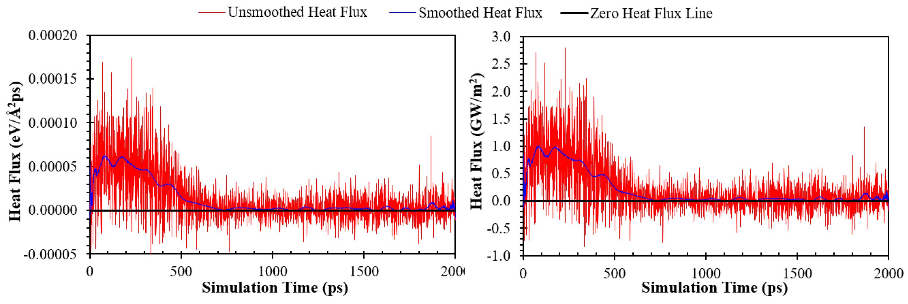
Figure 3.
Changing of density and cell length of the simulation Case I during the NPT simulation. The experimental data are from Ref. [35].
Figure 3.
Changing of density and cell length of the simulation Case I during the NPT simulation. The experimental data are from Ref. [35].
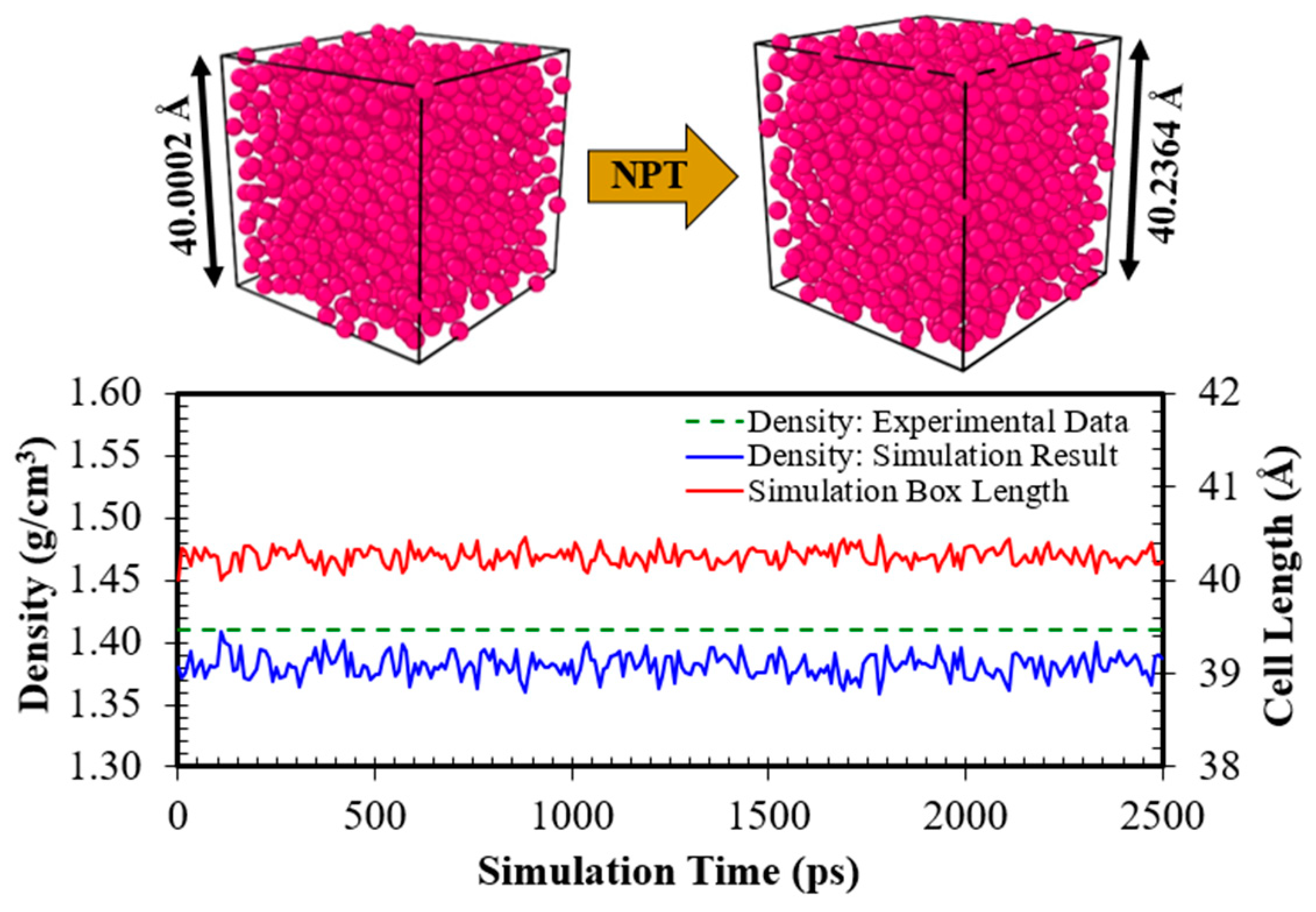
Figure 4.
Comparison between experimental and simulated RDFs of liquid argon. The experimental data are from Ref. [41].
Figure 4.
Comparison between experimental and simulated RDFs of liquid argon. The experimental data are from Ref. [41].
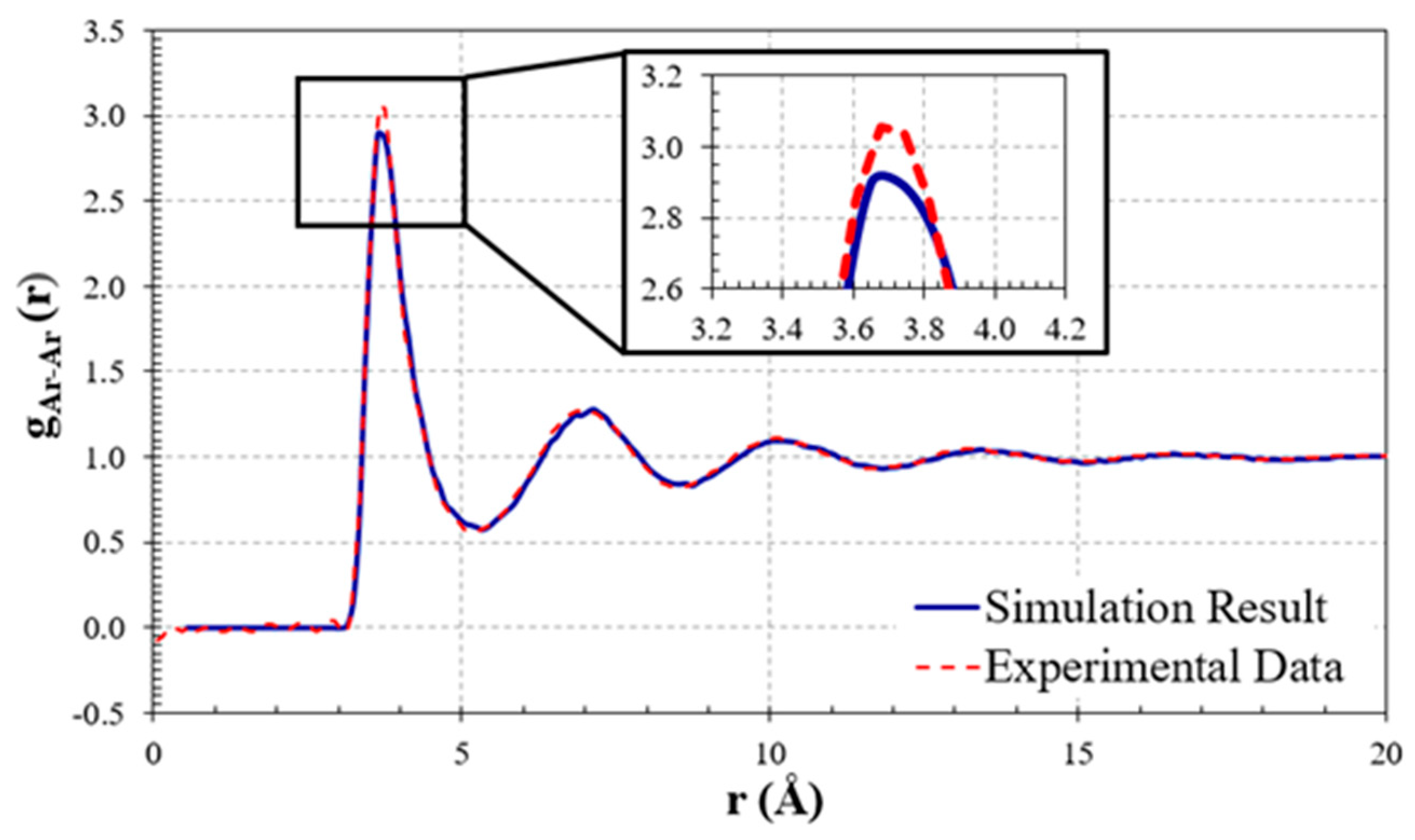
Figure 5.
Snapshot of the initial configuration of the simulation Case II.
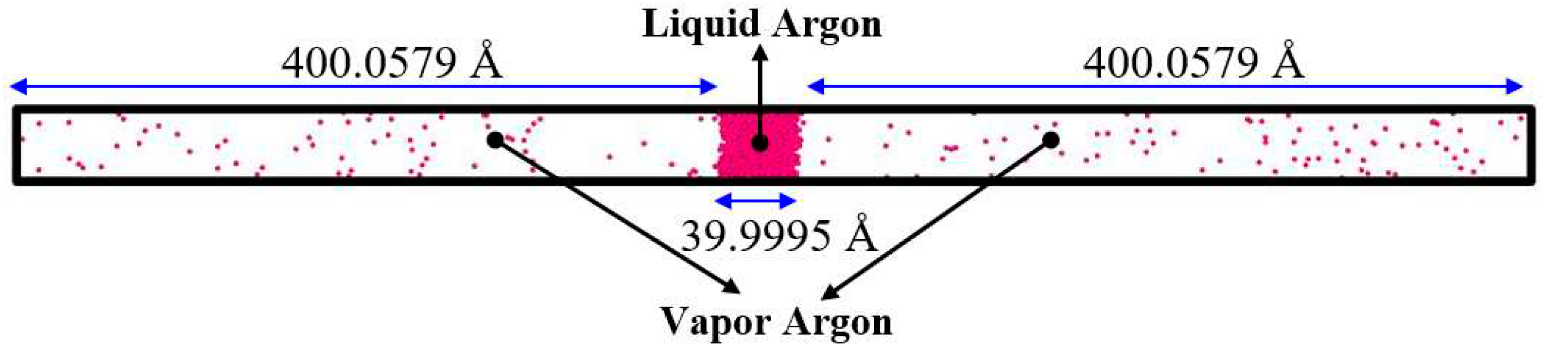
Figure 6.
Comparison between density profile along the Z– direction (at 2000 and 2500 ps) for the simulation Case II and the experimental data. The experimental data are from Ref. [35].
Figure 6.
Comparison between density profile along the Z– direction (at 2000 and 2500 ps) for the simulation Case II and the experimental data. The experimental data are from Ref. [35].
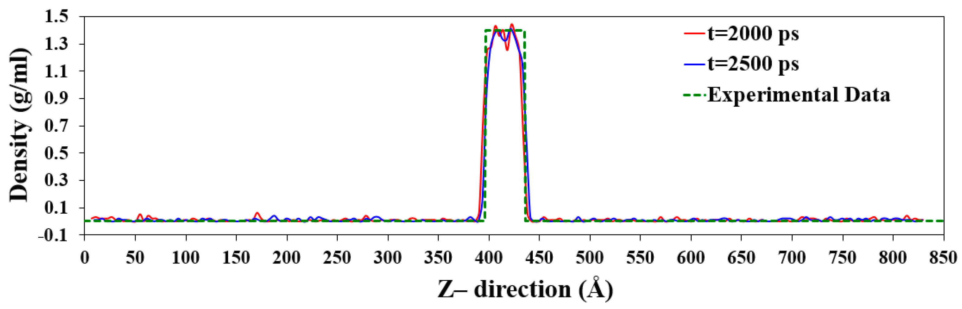
Figure 7.
Snapshots of density profiles of the simulation Case II at 2000, 2250, and 2500 ps.
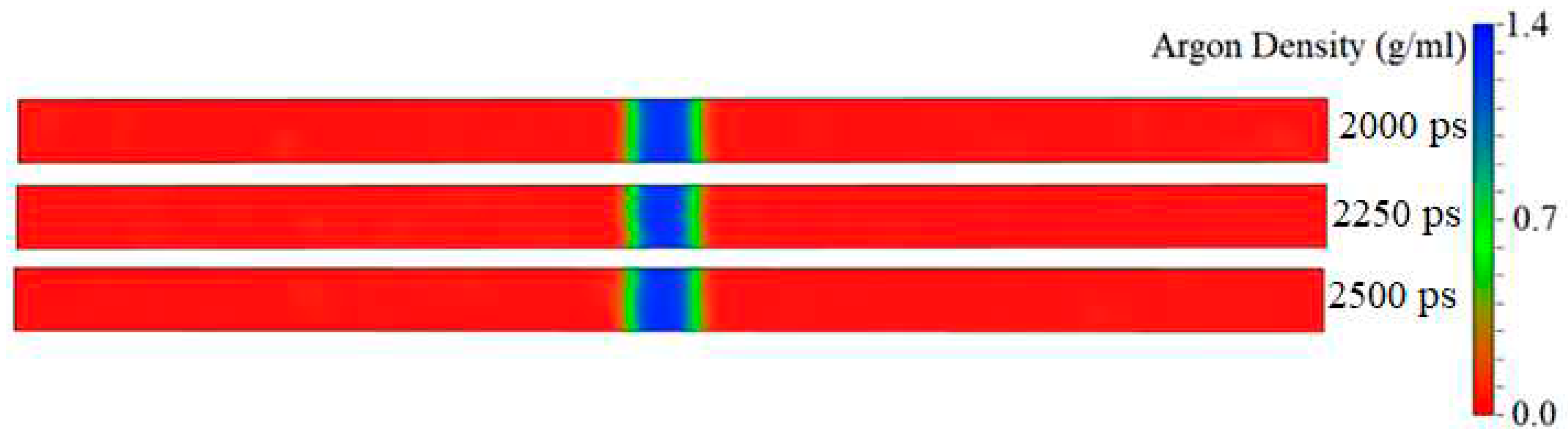
Figure 8.
Changes in the onset time of explosive boiling versus increasing the surface ratio (the wetted surface area / the nominal surface area) for various topologies.
Figure 8.
Changes in the onset time of explosive boiling versus increasing the surface ratio (the wetted surface area / the nominal surface area) for various topologies.
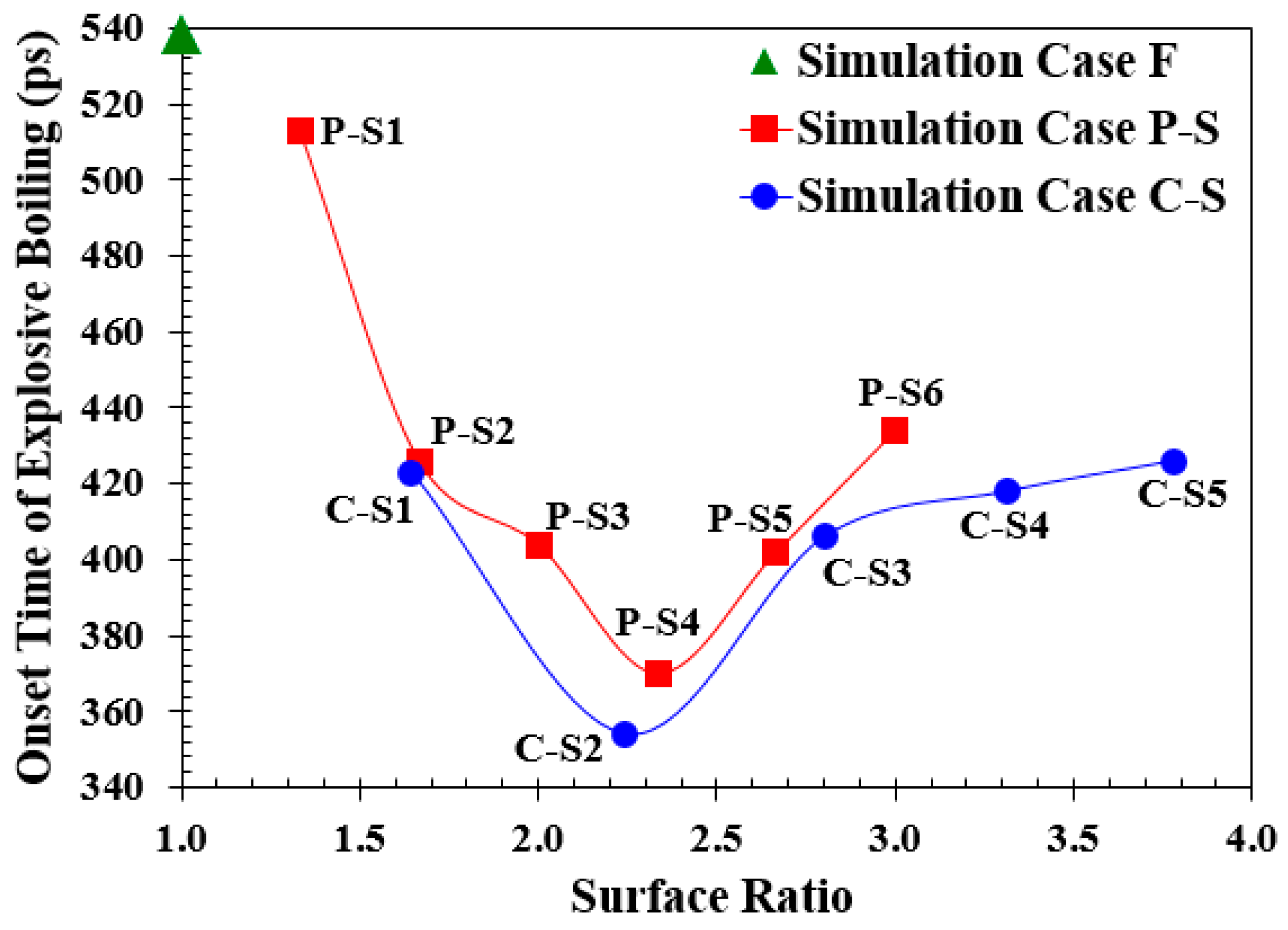
Figure 9.
Variation in heat flux (eV/Å2 ps) of fluid argon domain on solid copper surfaces for various parallel nanowall surfaces.
Figure 9.
Variation in heat flux (eV/Å2 ps) of fluid argon domain on solid copper surfaces for various parallel nanowall surfaces.
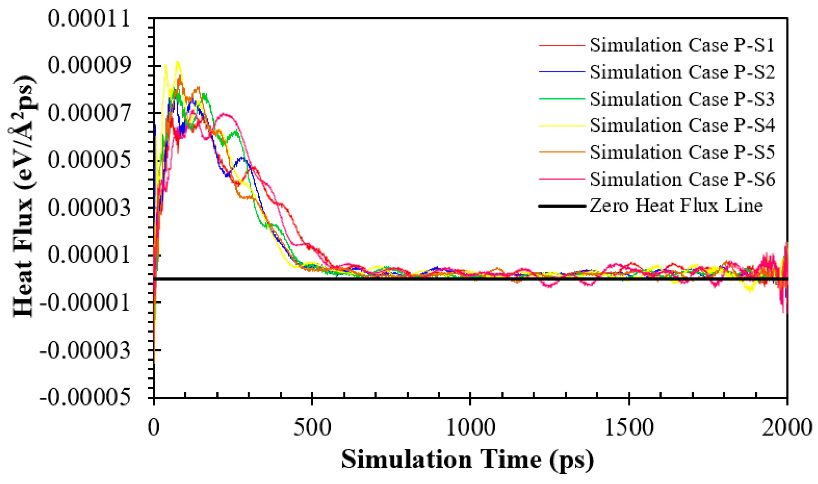
Figure 10.
Comparison of potential energy per Ar atoms distributions and number of Ar atoms with high potential energy (-0.04 – -0.08 eV/atom) for the ideally smooth surface and various parallel nanowall surfaces.
Figure 10.
Comparison of potential energy per Ar atoms distributions and number of Ar atoms with high potential energy (-0.04 – -0.08 eV/atom) for the ideally smooth surface and various parallel nanowall surfaces.
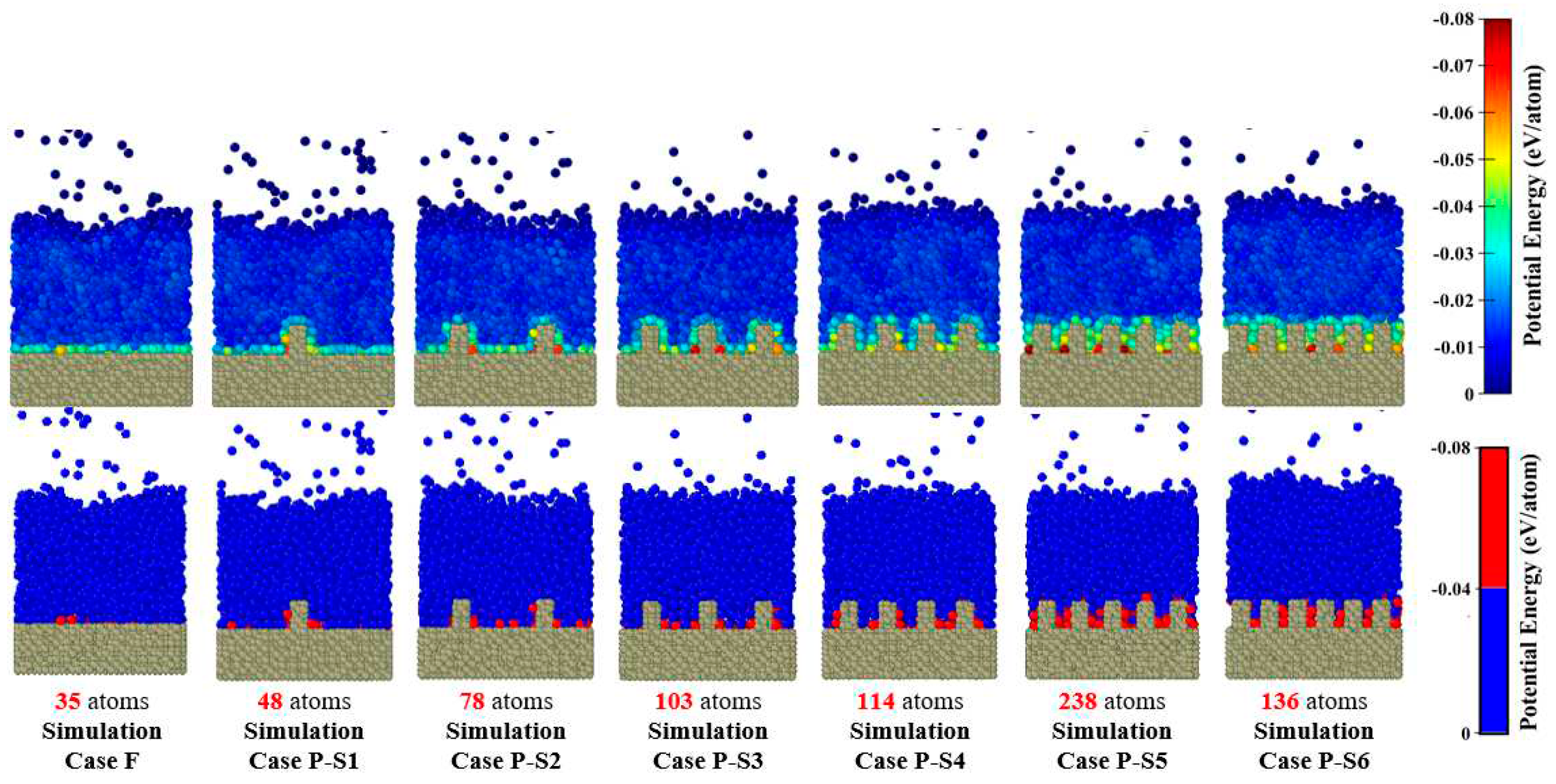
Figure 11.
Projections of trajectory lines of Ar atom motion between the nanowalls for various parallel nanowall surfaces.
Figure 11.
Projections of trajectory lines of Ar atom motion between the nanowalls for various parallel nanowall surfaces.
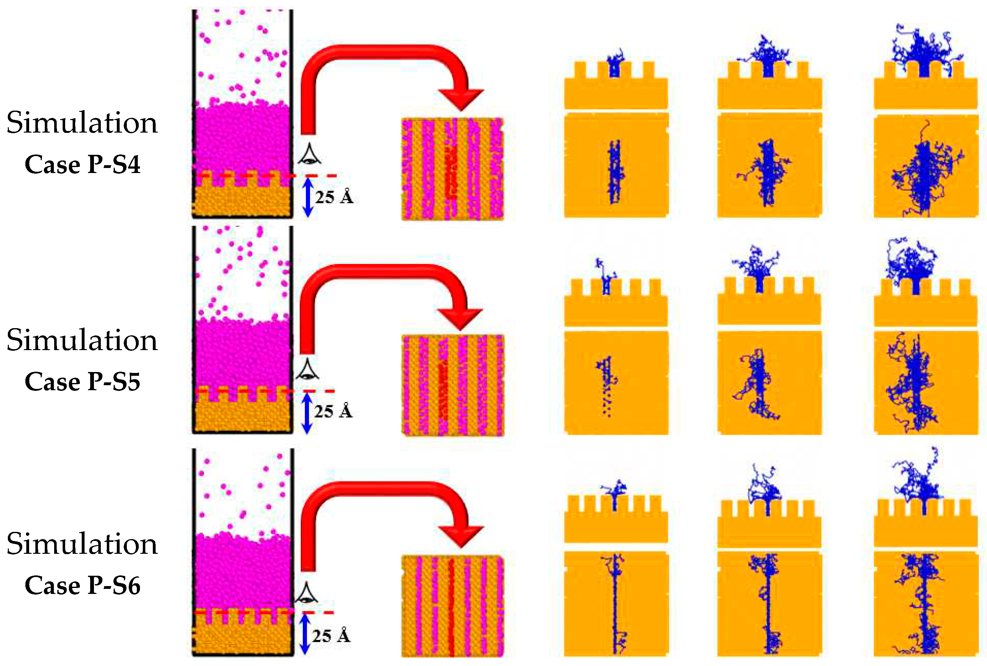
Figure 12.
Variation in heat flux (eV/(Å2ps)) of fluid argon domain on solid copper surfaces for the simulation Case F, P-S4, and C-S2.
Figure 12.
Variation in heat flux (eV/(Å2ps)) of fluid argon domain on solid copper surfaces for the simulation Case F, P-S4, and C-S2.
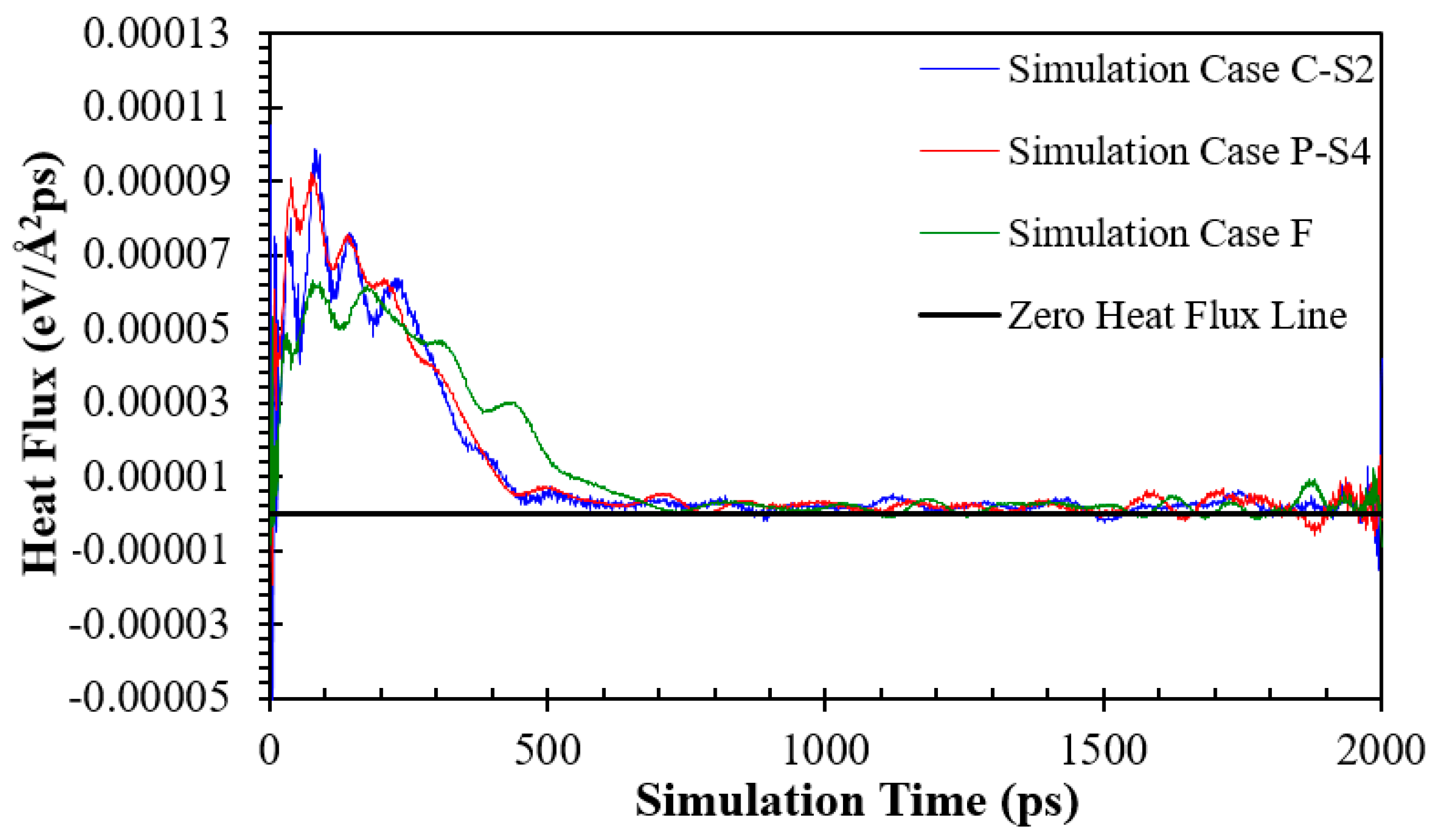
Figure 13.
Temperature history of fluid argon domain for the simulation Cases F, P-S4, and C-S2.
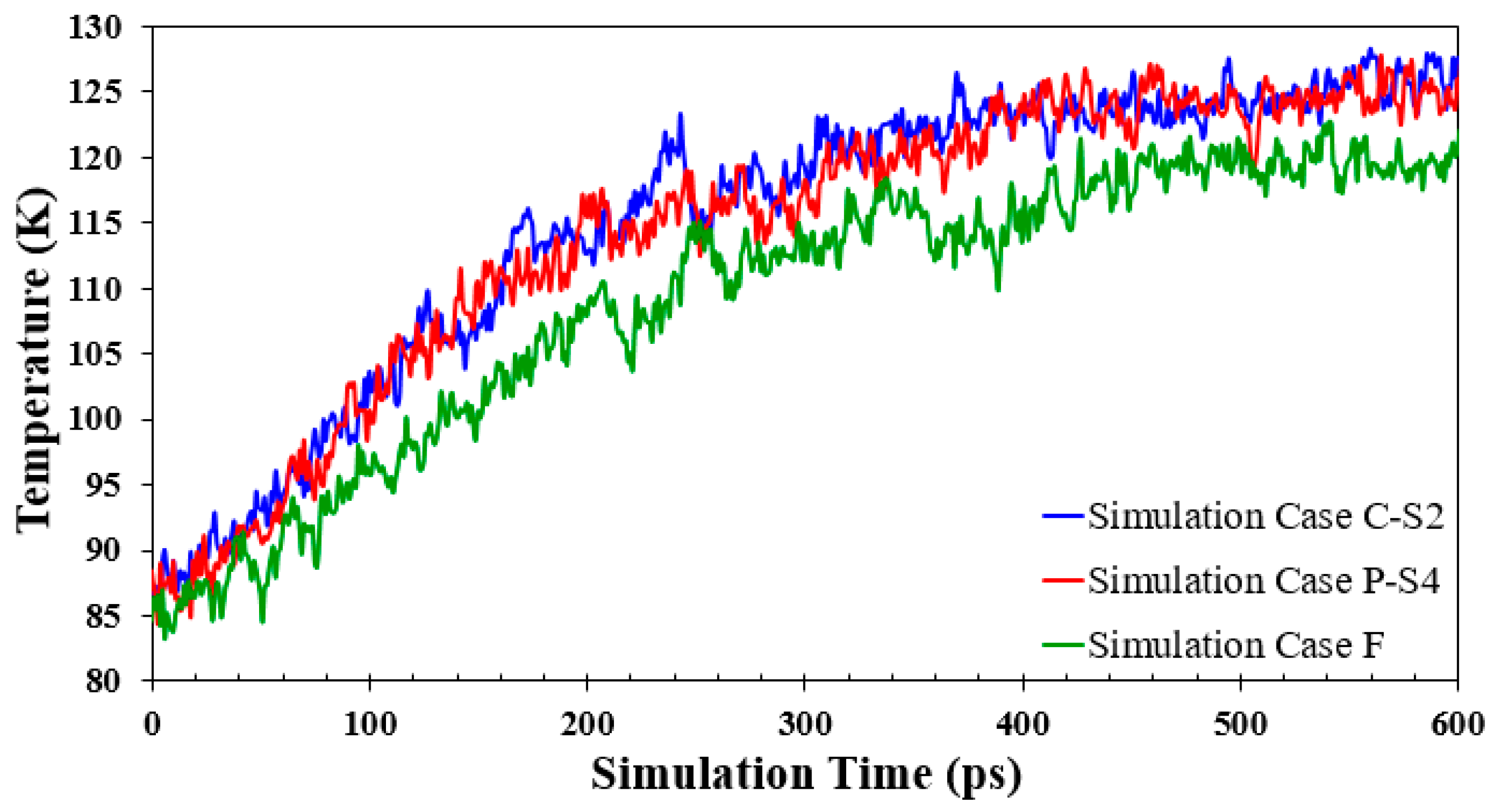
Figure 14.
The number of liquid and vapor Ar atoms as a function of time for the simulation Cases F, P-S4, and C-S2.
Figure 14.
The number of liquid and vapor Ar atoms as a function of time for the simulation Cases F, P-S4, and C-S2.
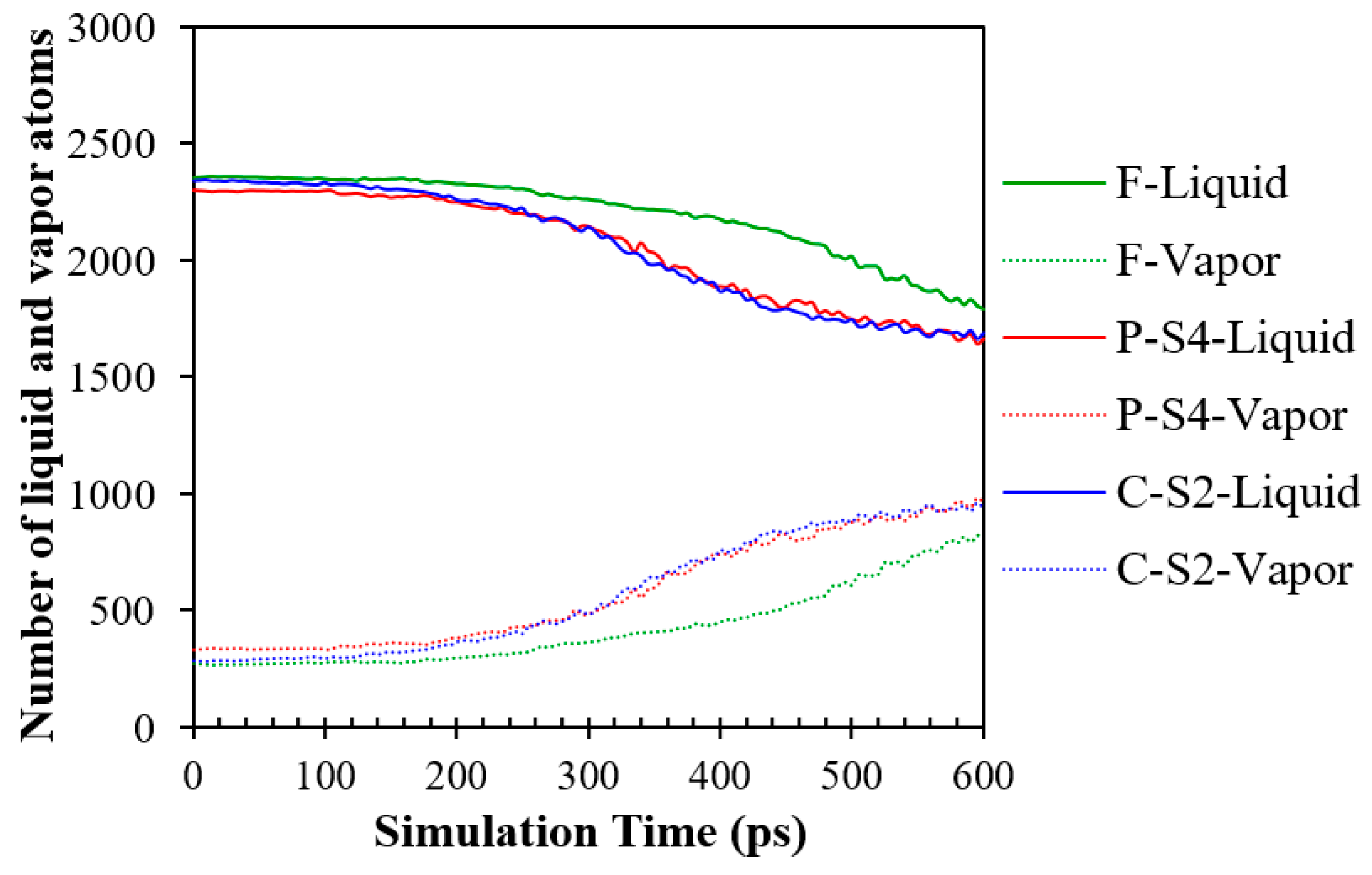
Figure 15.
Density profile of the fluid argon domain in the Z-direction for simulation Cases F, P-S4, and C-S2 at various times.
Figure 15.
Density profile of the fluid argon domain in the Z-direction for simulation Cases F, P-S4, and C-S2 at various times.
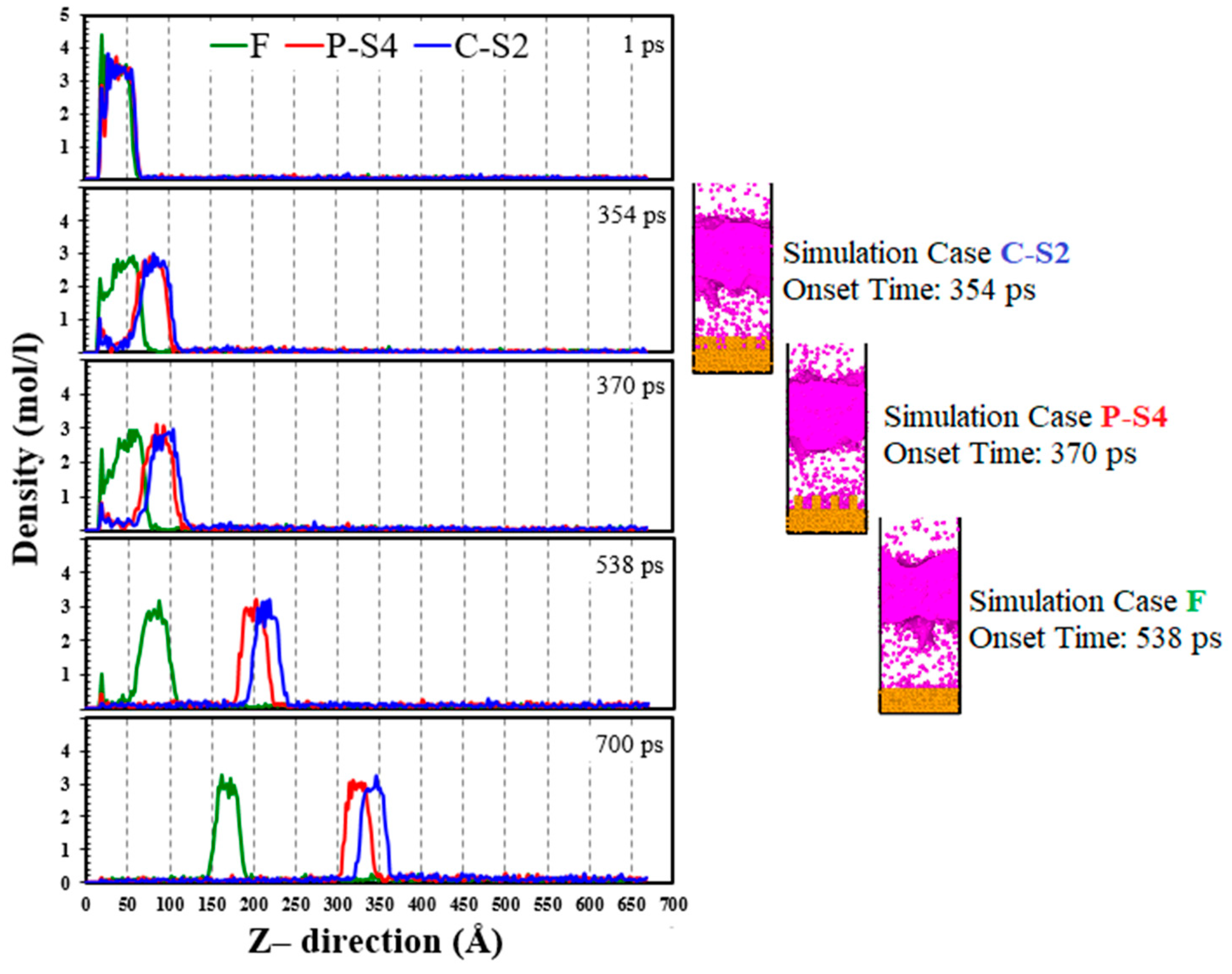
Figure 16.
Changes in the onset time of explosive boiling versus increasing the nanowall height for the cross nanowall topology.
Figure 16.
Changes in the onset time of explosive boiling versus increasing the nanowall height for the cross nanowall topology.
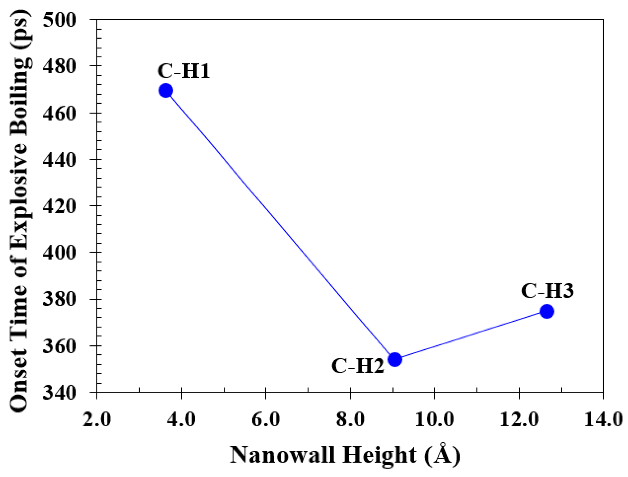
Figure 17.
Variation in heat flux (eV/(Å2ps) of fluid argon domain on solid copper surfaces for the simulation Case C-H1, C-H2, and C-H3.
Figure 17.
Variation in heat flux (eV/(Å2ps) of fluid argon domain on solid copper surfaces for the simulation Case C-H1, C-H2, and C-H3.
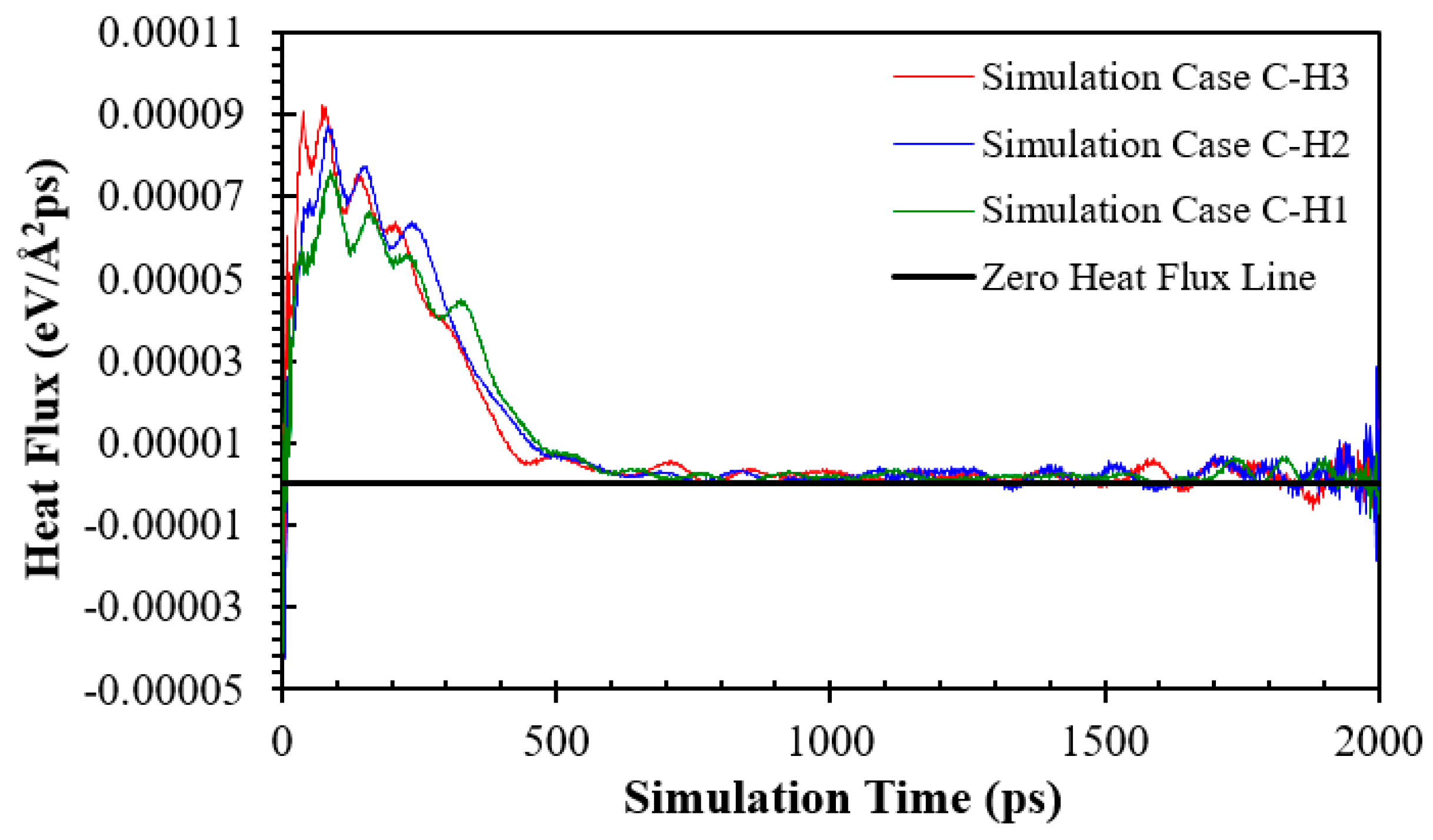
Figure 18.
Temperature history of fluid argon domain for the simulation Cases C-H1, C-H2, and C-H3.
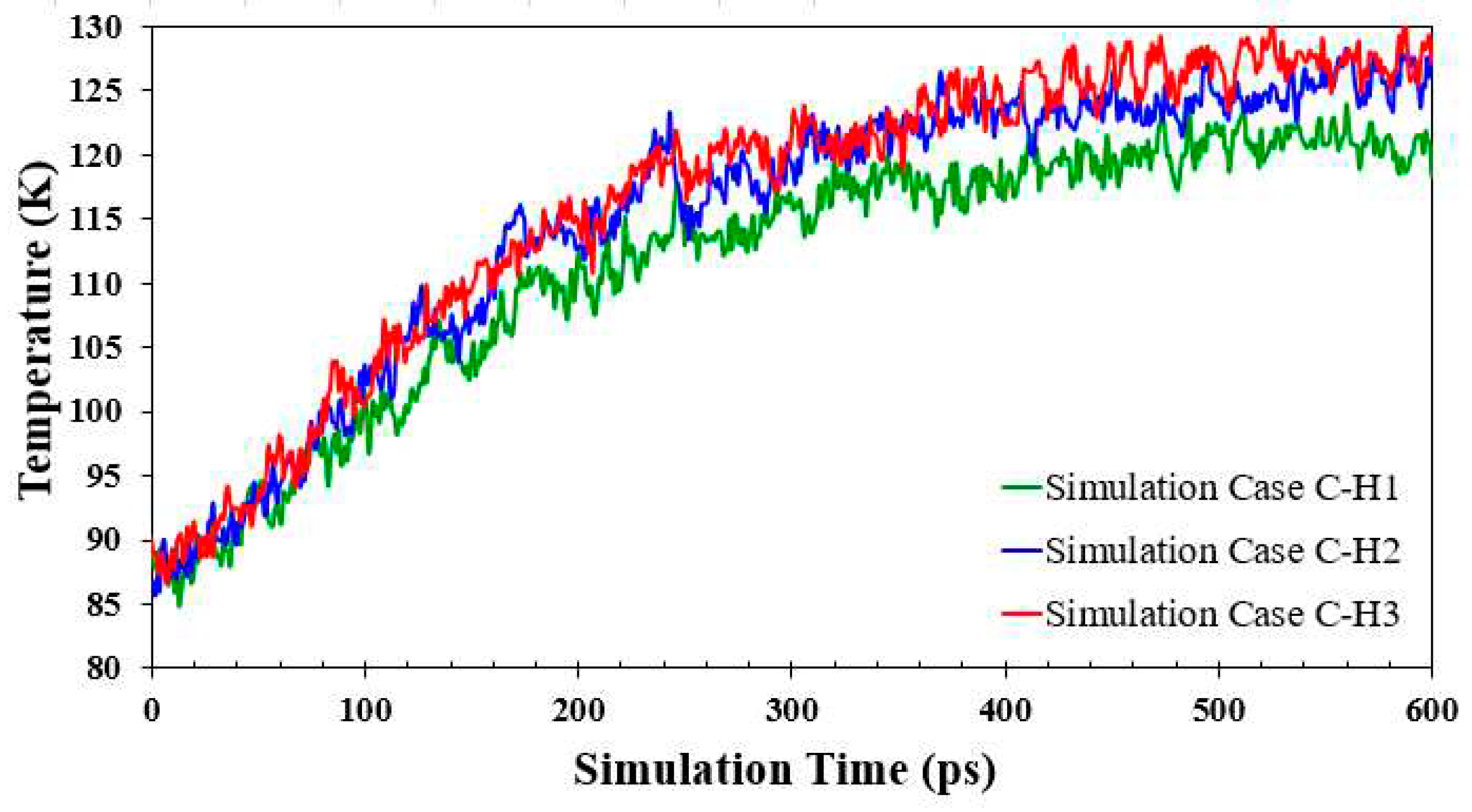
Figure 19.
Comparison of potential energy per Ar atoms distributions and number of Ar atoms with high potential energy (-0.04 – -0.08 eV/atom) for the simulation Cases C-H1, C-H2, and C-H3.
Figure 19.
Comparison of potential energy per Ar atoms distributions and number of Ar atoms with high potential energy (-0.04 – -0.08 eV/atom) for the simulation Cases C-H1, C-H2, and C-H3.
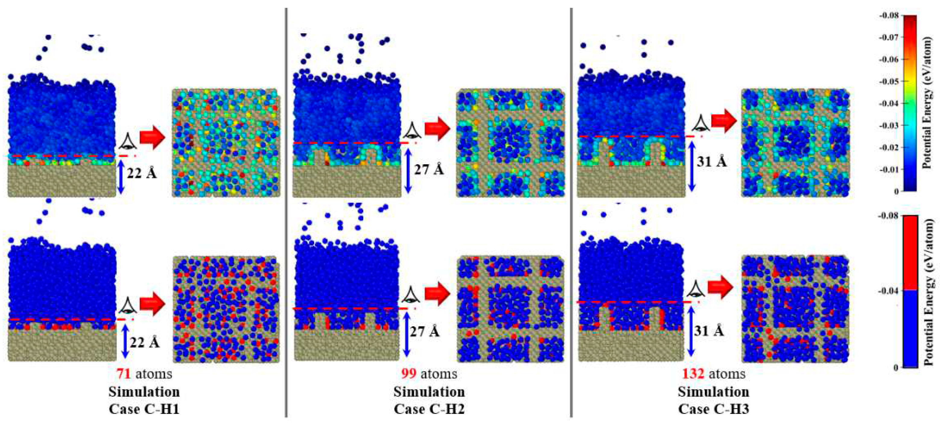

Table 1.
Literature overview of MDS studies of normal and explosive boiling on nanostructured surfaces.
Table 1.
Literature overview of MDS studies of normal and explosive boiling on nanostructured surfaces.
 |
 |
 |
||||
| Spherical nanopillar | Cylindrical nanopillar | Conical nanopillar | ||||
 |
 |
|||||
| Cubical nanopillar | Cubical nanowall | |||||
| Study | Boiling Mode | Mediums of Fluid / Solid | Nanostructure | Substrate Temperature (K) |
||
| Topology (Shape) | Configuration (Size)* | |||||
| Morshed et al. [1] | Normal / Explosive | Argon/ Platinum |
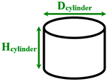
Separated cylindrical nanopillars | Dcylinder= 1.013 Hcylinder= 1.754–4.782 |
130 and 300 | |
| Seyf and Zhang [6] | Normal / Explosive | Argon / Copper |
Separated spherical nanopillars | Dsphere=1–3 | 170 and 290 | |
| Seyf and Zhang [14] | Explosive | Argon / Aluminum and Silver |
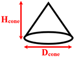
Separated conical nanopillars | Dcone= 1 Hcone= 2–5 |
270 | |
| Wang et al. [15] | Normal / Explosive | Argon / Aluminum |
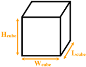
Separated cubical nanopillars | Wcube= 1.8 Lcube= 1.8 Hcube= 1.8225–4.455 |
150 and 310 | |
| Fu et al. [16] | Explosive | Water / Copper |
Separated cubical nanopillars | Wcube= 1.444–2.166 Lcube= 1.444–2.166 Hcube= 1.444–2.166 |
1000 | |
| Zhang et al. [17] | Explosive | Argon / Copper |
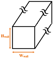
Parallel cubical nanowalls | Wwall= 1.808 Hwall= 1.266–3.434 |
350 | |
| Liu et al. [9] | Explosive | Argon / Copper |
Random roughness surface | – | 300 | |
| Zhang et al. [10] | Explosive | Water / Copper |
Separated cubical nanopillars | Wcube= 1.444 Lcube= 1.444 Hcube= 1.444 |
800 | |
| Liao and Duan [19] | Explosive | Argon / Gold |
Parallel cubical nanowalls | Wwall= 0.612 Hwall= 0.816-2.040 |
120-240 | |
| Liu et al. [20] | Explosive | Argon / Copper |
Random roughness surface | – | 300 | |
| Qasemian et al. [18] | Explosive | Argon / Aluminum and Copper |
Separated conical nanopillars | Dcone= 2.8 Hcone= 2 |
350 | |
| Zhou et al. [11] | Explosive | Water / Copper |
Separated spherical and cylindrical nanopillars | Dsphere=1–1.44 Dcylinder=6 Hcylinder=1.8 |
1000 | |
* All dimensions are reported in nm (nanometer).
Table 2.
Force field parameters of different atom pairs.
| Atom pairs | (Å) | (eV) |
| Cu-Cu | 1.9297 | 0.2047 |
| Ar-Ar | 3.4050 | 0.0104 |
| Ar-Cu | 2.6674 | 0.0065 |
Table 3.
Simulation cases and corresponding topologies and configuration parameters.
 |
 |
 |
 |
| Surface F | Surface P | Surface C | |
| The top and side schematic views of different copper surface topologies. | |||
| Simulation Case1 | Spacing (Å) | Height (Å) | Surface ratio2 |
| 1. Simulation Cases A: Different topologies with different Spacing: | |||
| F | – | – | 1 |
| P-S1 | 50.6058 | 9.0368 | 1.3333 |
| P-S2 | 23.4956 | 1.6667 | |
| P-S3 | 14.4588 | 2.0000 | |
| P-S4 | 9.0368 | 2.3333 | |
| P-S5 | 7.2294 | 2.6667 | |
| P-S6 | 5.4220 | 3.0000 | |
| C-S1 | 50.6058 | 1.6444 | |
| C-S2 | 23.4956 | 2.2445 | |
| C-S3 | 14.4588 | 2.8000 | |
| C-S4 | 9.0368 | 3.3111 | |
| C-S5 | 7.2294 | 3.7778 | |
| F | – | 1 | |
| P-S1 | 50.6058 | 1.3333 | |
| 2. Simulation Cases B: Cross nanowall surfaces with different Heights: | |||
| C-H1 | 23.4956 | 3.6147 | 1.4978 |
| C-H2 | 9.0368 | 2.2445 | |
| C-H3 | 12.6515 | 2.7422 | |
1For convenience of reference, the simulation cases were labeled using two parts: the first part of the case name indicates the topology of the copper surface (F: smooth surface, P: parallel nanochannel surface, and C: cross nanochannel surface), and the second part of the case name shows the variable parameter for different configurations (S: spacing and H: height). 2Surface ration= (the wetted surface area)/(the nominal surface area).
Disclaimer/Publisher’s Note: The statements, opinions and data contained in all publications are solely those of the individual author(s) and contributor(s) and not of MDPI and/or the editor(s). MDPI and/or the editor(s) disclaim responsibility for any injury to people or property resulting from any ideas, methods, instructions or products referred to in the content. |
© 2024 by the authors. Licensee MDPI, Basel, Switzerland. This article is an open access article distributed under the terms and conditions of the Creative Commons Attribution (CC BY) license (https://creativecommons.org/licenses/by/4.0/).
Copyright: This open access article is published under a Creative Commons CC BY 4.0 license, which permit the free download, distribution, and reuse, provided that the author and preprint are cited in any reuse.


