
Submitted:
03 January 2024
Posted:
18 January 2024
You are already at the latest version
Abstract
The precise mathematical description of gaze patterns is still an unsettled matter of debate. This can, consequently, affect the analysis of this type of data in its practical applications. In this scope, we show evidence that a Lévy-flight description of eye-gaze trajectories is not only appropriate but its scale invariant properties are remarkably useful to assist in diagnosing children with Attention Deficit and Hyperactivity Disorder (ADHD), alongside with the usual cognitive tests. Using this picture, we find that the distribution of the characteristic exponent of Lévy-flights statistically is different in children with ADHD. Furthermore, we observe that these children deviate from a strategy that is considered optimal for searching processes, in contrast to non-ADHD children. We focus on the case where both eye-tracking data and data from a cognitive test are present and show that the study of gaze patterns in children with ADHD can help in identifying this condition. Since eye-tracking data can be gathered during cognitive tests without needing extra time-consuming specific tasks, we argue that it is in prime position to provide assistance in the arduous task of ADHD diagnosing.
Keywords:
ADHD diagnosis
; Eye-tracking data
; Gaze trajectories
; Lévy-flights
; Lévy foraging hypothesis.
1. Introduction
The study of time-series is central to mathematics and physics with an extensive range of interdisciplinary applications. A class of time-series that has gathered increased interest in recent years are the ones with rare extreme events, such as eye-tracking time-series, i.e. the recording of human eye-movements while looking at a screen.
Some of the reasons that make gaze dynamics so appealing to study are its interesting theoretical properties, namely relatively sparse high velocity events, and the currently standing question of the best mathematical equation describing gaze trajectories. There are two schools of thought, even though they are not always juxtaposed [1]. The common assumption outside the mathematics literature is that there are two alternating types of eye-movements [2]: fixations, during which an individual’s gaze is centered around one specific point with very little deviation and, presumably, visual information is being extracted and saccades, fast re-locations of gaze from one point to another.
Mathematically, it is posited that the visual and oculomotor systems may conform to Lévy-flight model [3]. This has been empirically supported by the work presented in Ref. [4] with the emergence of superdiffusive dynamics arising in this context [5]. In fact, superdiffusive nature of gaze trajectories has been presented over two decades ago [6]. In that study, the authors propose that visual scanpaths generated under natural circumstances bear similarities to Lévy-flights, indicating a power-law dependency in their magnitude distribution.
In the context of visual scanpaths, this indicates that a viewer’s attention may occasionally make extensive shifts across the scene, intermixed with smaller, local movements. It has also been shown that Lévy-flights reproduce well human gaze patterns over a saliency map [7].
This is extremely similar to the foraging subclass of stochastic processes, i.e. time-series where an agent is searching food, water or, in our particular case, visual information.
Indeed, it is speculated that there is Lévy-flights describe foraging strategies observed in nature in all its contexts [8]. These strategies manifest the movement of bacteria [9,10], the search for fish by albatrosses [11] or the foraging for food by sharks in the ocean [12]. This pattern is also present in several human tasks, such as the exploration of the Walt Disney Resort by children [13], the exploration of virtual environments [14] and was even proposed as a mathematical model to the way humans search memories [15].
Using this framework, eye-tracking experiments found the characteristic Lévy exponent () to be approximately (or using a different convention than the one we are using here) [16], regardless of the level of difficulty of the visual task.
While it is still an open question if eye-gaze trajectories follow Lévy-like processes or other, such as intermittent process [17], this finding supports the notion that the Lévy-flight model can be applied visual scanpaths in various contexts, and it emphasizes the potential relevance of the scaling exponent in characterizing eye movements. The question of universality is not new and it has been argued that an optimal for search strategies is [18], and, indeed, empirical testing showed that in the case of foraging animals the Lévy exponent turned out to match the optimal value [19].
Besides the theoretical question of the best mathematical description of gaze trajectories, eye-tracking data has been gaining popularity due to its wide range of applications in health sciences. It can be used to determine an individuals’ age, gender, ethnicity [20], personality traits such as extroversion, curiosity, neuroticism, openness, agreeableness [21], Intelligent Quotient (IQ) [22], as well as being able to detect conditions such as Alzheimer’s [23] or autism [24].
Due to its diagnosis’ challenges, of the conditions where eye-tracking might have the most impact is Attention-Deficit/Hyperactivity Disorder (ADHD). It has been suggested that around 20% of ADHD diagnosis could be false positives [25] with an unknown expected percentage of children classified as false negatives. This difficulty in diagnosing ADHD has led to significant variations in its prevalence, which has been reported to affect from to of children [26]. Another difficulty of the ADHD diagnosis is that it involves a lengthy series of cognitive tests and interviews.
While the condition is not curable, an early diagnosis is important to mitigate its impact, provide adequate medication and to teach people affected by it coping skills. This is increasingly important when taken into account that it is the most prevailing neurodevelopmental disorders among children and adolescents, impacting academic performance, overall well-being, and social interactions in children [27]. When unmitigated, the impact can be felt even adulthood, with affected individuals having shorter more often discordant romantic relationships [28].
In the important task of assisting ADHD diagnosis, eye-tracking has been applied in reading tasks [29], during memory performance tests [30] or while playing in virtual reality [31]. We intend to add to this body of literature by justifying and applying a Lévy-flight inspired methodology. These methods also have the advantage of being scale invariant and thus, in a time when phone cameras can start tracking eye-movements [32], the robustness of this approach to different scales being employed is a definite advantage.
2. Data and methods
2.1. Data: Eye-gaze trajectories and ADHD cognitive test
The dataset we use in this study originates from an experiment detailed in Ref. [33], focusing on visuospatial working memory and involving participants both with and without ADHD. The experiment included 50 participants (47 with complete data) engaged in a Sternberg-type delayed visuospatial working memory task, adapted from Ref. [33].
This working memory task showed one or two dots in the screen, with dots positioned in one of sixteen locations within a 4×4 grid. The goal of the participants was to memorize the position of the dots, while some distractors (images or videos) were shown between the time when the participants first saw the dots and the time when they were finally evaluated on memorizing the dots’ position.
The assumption nested in this experiment is that children with ADHD are more prone to being distracted and thus will fail this test more often. This assumption also arises in the studies from Ref. [34,35] which used the WISC-III cognitive test and found that the ADHD group scored significantly lower on Freedom from Distraction (FD), which, in the context of the WISC-III cognitive test, is composed by the Digit Span and Arithmetic subtests. Results of the WISC-III cognitive test were also provided in this dataset.
Other parameters that might affect a child’s performance in the memory test were controlled for, namely age, IQ.
Furthermore, eye movements were recorded for the duration of the experiment.
2.2. Lévy-flights and superdiffusion
A Lévy-flight is a type of random walk named after the French mathematician Paul Lévy, which has seen a wide range of applications since the 1980’s [36]. As a random walk, it describes a series of positions across time via the equation
where is the position of the particle at time t, the initial position, the position increments or steps and is the number of steps taken up to time t.
The distribution of the increments, , is what distinguishes a Lévy-flight from other random walks such as Brownian motion [37]. Unlike the latter, where are normally distributed, in a Lévy-flight the steps follow a heavy-tailed distribution, such as a Lévy distribution, characterized by its power-law tail.
The probability density function (PDF) of a Lévy distribution is given by:
where the coefficient determines the heaviness of the tails [38]. When , the process converges to a Gaussian random walk [39] by the central limit theorem, while for values the process does not yield a normalized probability distribution. For , the distribution has no convergent mean and no variance and for , the distribution has a finite mean but not when it comes variance [40]. This is why this type of distribution escapes the range of applications of the central limit theorem (that requires finite mean and variance) and does not converge to a Gaussian random walk when the steps are measure over large time-windows .
The fact that, asymptotically, Lévy-flights lead to a different behaviour than a Wiener process is well documented in the literature with this behaviour being known as superdiffusivity [5], a phenomenon characterized by a higher-than-normal rate of spreading or dispersion compared to classical diffusion.
In a superdiffusive process, the mean-squared displacement (MSD) of a particle grows faster than linearly with time. The MSD is defined as:
For classical diffusion, the MSD grows linearly with time (), but in superdiffusion, the growth is faster than linear with
with, in the context of Lévy-flights,
Multi-Fractal Detrended Fluctuation Analysis (MFDFA) is a technique that can be used to estimate the parameter . It is an extension of the detrended fluctuation analysis (DFA) method, allowing for the assessment of the multifractal nature of complex systems. The details of the algorithm can be found in Ref. [41].
2.3. Machine learning classification methods
In order to classify individuals as belonging to the ADHD category or not, based on parameters such as age, test performance or features of their gaze trajectories, we employ three different machine learning methods for this type of classification task.
2.3.1. Logistic regression
Logistic Regression is one of the most simple binary classification methods. In it, the logistic function, also known as the sigmoid function, is used to map the output of a linear combination of features to a value between 0 and 1.
The logistic function is defined as:
where z is the linear combination of input features and model parameters:
In our case, the variables represent metrics such as age, IQ or eye-tracking derived metrics that we will use to distinguish between children with ADHD from those without the condition.
Conversely, the fi-coefficients associated with are estimated via a maximum likelihood estimation and each coefficient can be interpreted as the weight of the variable to the model, with being the intercept of the model.
After estimating the -coefficients, one can calculate the probability of an instance characterized by a variable array x belonging to the positive class:
where Y is the binary target variable, where 1 corresponds to the case of a children with ADHD and 0 otherwise.
The logistic regression model predicts the class label by thresholding the predicted probability as follows:
2.3.2. Support Vector Machines
Support Vector Machines (SVMs) is another class of supervised algorithms used for classification tasks.
In this context, this algorithm has the goal of finding the hyperplane that best separates the data into different classes. In our case, that creates two mutually exclusive regions where, given value of the feature vector , an instance is assigned a value or .
In the most simple case when an hyperplane exists that perfectly separates between classes (ADHD and non ADHD in our case), the hyperplane defined by the SVM algorithm has the form
where, similarly to the -coefficients in the logistic regression, the vector represent the weight vector and b represents the bias term (similarly to in the logistic regression).
In that case, the classification decision is made based on the sign of :
In most practical applications it is not possible to find a hyper plane that perfectly separates between classes and some overlap exists even after finding an appropriate hyperplane. In this case, SVMs can use kernel functions to map the input features into a higher-dimensional space. The decision function becomes:
where is a kernel function and are the Lagrange multipliers.
The choice of an appropriate kernel functions depends on the problem. Common kernels include the linear kernel , the polynomial kernel , and the radial basis function kernel , with s being a width parameter.
2.3.3. Decision Trees and Random Forests
A decision tree is a non-linear, non-parametric model used for both classification and regression tasks. A decision tree recursively partitions the feature space (where x lies) to create homogeneous subsets until a stopping criterion is met. The decision at each node is typically based on optimizing impurity measures such as Gini impurity or entropy.
Mathematically, given a vector encapsulating the relevant metrics for a classification task and a series of corresponding labels . A decision tree can be represented by a function that maps feature vectors to predicted labels:
where N is the number of terminal nodes, the predicted value at terminal node i, the region corresponding to terminal node i, and is the indicator function.
A Random Forest is method that groups multiple decision trees and combines their predictions. Random Forests improve generalization and reduce overfitting compared to individual decision trees. Each tree is trained on a subset of the data and may use a random subset of features at each split. The final prediction a majority vote of individual tree predictions.
3. Results: Lévy-flight exponents classify ADHD children
From here onwards we will analyse the data from the one-dot memoranda task. In this task, participants saw one dot in a 4x4 grid and had to memorize its position for seconds, a period of time when they were shown pictures and videos that served as distractors.
Since these distractors varied from trial to trial, for consistency reasons, the eye-tracking data that we analysed focus solely on gaze patterns of participants while looking at the 4x4 grid with one dot in it.
3.1. Eye-gaze dynamics and the Lévy-flight exponent
While the Lévy-flight framework diverges from the usual picture of two alternating process, one slow (called fixation in the occulomotor field), one fast (called saccades), in our case we can see that not only is it adequate but actually preferable.
In Figure 1 we observe two relevant features in the probability density function (PDF) of the distribution of the increment’s norm : firstly, we observe a power-law decay that is integral to the PDF and not just a small part of the tail of the PDF and, secondly, we do not observe a bi-modal velocity PDF that is often used as a justification for the assumption of two separate sub-processes of fixations and saccades.
We also see in Figure 2 the values of the mean, standard deviation, skewness and kurtosis of . We observe that they are quite disparate across experimental participants, often with variations of two orders of magnitude. One advantage of looking at the Lévy exponent (or for the scaling exponent ) is that this approach is scale invariant.
Why exactly this dataset has this feature of disparate scales is unclear, but some inconsistencies in the screen monitor distance have been noticed.
We observe as well in Figure 3 that the relation holds to a significant degree. Furthermore, in Figure 4 we compute the coefficient of determination (r-square). With values of r-square over , we observe that both in the estimation of via the PDF or in the case of via the relation corroborate the Lévy-flight assumption as a valid one.
3.2. Classifying ADHD without eye-tracking
Before investigating the impact of including a Lévy description of gaze movements in our classification model, we create a benchmark model using other metrics solely dependent on non eye-tracking related metrics. These are: the age of the children, the specific metrics from their WISC test, and their test performance. The accuracy of this model will subsequently be compared with the model including eye-tracking metrics.
To create the benchmark model we use the following variables: Age, full scale IQ (later excluded), arithmetic and digit span subtests of the WISC-III cognitive test and the one-dot memory test performance. While we have 50 test participants, 3 of the have incomplete data, leaving us with 47 test subjects.
The method tested are the ones already mentioned in Section 2, namely, Logistic Regression, SVMs, Decision Tree and Random Forest. Since we have a limited number of participants, we cannot use the common approach of fitting the parameter of the model in of the data and testing its accuracy in the remaining . Instead we use test different Cross Validations (CV) strategies.
In the first CV stategy, we do the aforementioned split, choosing at each time a different combination of participants to fit the parameters and test the accuracy of the model, in a process that is known as Stratified K-Fold (SKF) CV, with in this case. The final accuracy reported the average of 5000 combinations.
In the second type of CV, we apply a Leave One Out Cross-validation (LOOC), where we determine the parameters of a model with all the data except for 1 entry, that is left to be tested on. In our case, with 47 participants in total, this is done 47 times, each time fitting the parameters of the model on 46 entries and testing the model’s accuracy on 1 participant. Again, the reported accuracy is the average over all 47 realization.
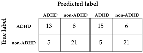
The results are presented in Table 1. There we see that in either case of CV strategies, the Logistic Regression is the best performing method, with an accuracy of . We find that, with this method, the accuracy is independent of the CV strategy and thus we will use the LOOC from now onwards, since we can more easily cover all possible CV combinations. The model results can also be seen in Table 2 (left), where other metrics such as precision of , specificity of and recall . The variable IQ was not included in the analysis as using it lead to overfitting and a decrease of CV accuracy.
3.3. Classifying ADHD with eye-tracking
When we calculate the value of the Lévy exponent we find that there is a discrepancy between children with and without ADHD. We see in Figure 5 that median of for children without ADHD is around , while for children with ADHD it centered between and and, according to the Mann-Whitney U test, this difference is significant with a p-value around .
While there is a difference in the median of the distribution of , this parameter alone does not yield a better accuracy than the benchmark model (around ). However, when incorporated with the other variables, it does increase the accuracy of the model, from to (see Table 2 on the right).
The increase in accuracy is reflected in the other metrics, namely, the precision (from to ) and specificity (from to ). Even though this increase is not very substancial, we must take into account that we have a limited number of data.
When this limitation takes place, typically adding more variables can lead to overfitting (the reason why we removed IQ from our analysis), which can actually decrease the overall accuracy. It is thus natural if with more data the accuracy increase would also be higher.
The value of is quite significant in the literature as it assumed to be the optimal exponent for searching processes [18] and the one more commonly found in nature, where biological evolution selects for more efficient strategies [19].
Children with ADHD having typically a lower coefficient indicates that they are more prone to having large, extreme relocations and exploring a larger area of the screen image. In this picture, gaze dynamics would mimic some of the body language of children with ADHD which often seem uneasy and with a tendency for extra movements when engaged in tasks that need concentration.
4. Conclusions
In this work, we have argue that Lévy-flights are good mathematical models of gaze dynamics and that its characteristic exponent is distributed differently between ADHD and non-ADHD children.
Our findings show that, having typically a smaller exponent, ADHD children explore more remote areas of images, which might be a consequence of their attention deficit.
We observe that the Lévy-flight description of gaze dynamics can improve the classification accuracy that is obtained when using a cognitive test. While the improvement is not very substantial, this also stems from the fact that we have a limited amount of data, and, when that is the case, adding extra variables to an already multi-variable model can lead to overfitting or to a reduced marginal accuracy gains.
Our approach also has the advantage of being scale independent. This means that it is not as sensitive to particular experimental parameters, such as the eye-tracker’s native frequency or the screen distance, as other approaches. Consequently, our approach could be used in eye-trackers with different characteristics and operated outside strict laboratory conditions. This is of particular importance for the diagnosis of ADHD in children, who typically present challenges for laboratory experimental setups.
References
- Lencastre, P.; Bhurtel, S.; Yazidi, A.; e Mello, G.B.; Denysov, S.; Lind, P.G. EyeT4Empathy: Dataset of foraging for visual information, gaze typing and empathy assessment. Scientific Data 2022, 9, 752. [Google Scholar] [CrossRef]
- Takahashi, M.; Sugiuchi, Y.; Na, J.; Shinoda, Y. Brainstem circuits triggering saccades and fixation. Journal of Neuroscience 2022, 42, 789–803. [Google Scholar] [CrossRef]
- Dubkov, A.A.; Spagnolo, B.; Uchaikin, V.V. Lévy flight superdiffusion: an introduction. International Journal of Bifurcation and Chaos 2008, 18, 2649–2672. [Google Scholar] [CrossRef]
- Rhodes, T.; Kello, C.T.; Kerster, B. Intrinsic and extrinsic contributions to heavy tails in visual foraging. Visual Cognition 2014, 22, 809–842. [Google Scholar] [CrossRef]
- Błażejczyk, P.; Magdziarz, M. Stochastic modeling of Lévy-like human eye movements. Chaos 2021, 31. [Google Scholar] [CrossRef]
- Brockmann, D.; Geisel, T. The ecology of gaze shifts. Neurocomputing 2000, 32-33, 643–650. [Google Scholar] [CrossRef]
- Boccignone, G.; Ferraro, M. Modelling gaze shift as a constrained random walk. Physica A: Statistical Mechanics and its Applications 2004, 331, 207–218. [Google Scholar] [CrossRef]
- Viswanathan, G.M.; Raposo, E.; Da Luz, M. Lévy flights and superdiffusion in the context of biological encounters and random searches. Physics of Life Reviews 2008, 5, 133–150. [Google Scholar] [CrossRef]
- Ariel, G.; Rabani, A.; Benisty, S.; Partridge, J.; Harshey, R.; Be’Er, A. Swarming bacteria migrate by Lévy Walk. Nature communications 2015, 6, 1–6. [Google Scholar] [CrossRef] [PubMed]
- Yan, X.F.; Ye, D.Y. Improved bacterial foraging optimization algorithm based on Levy flight. Computer System & Applications 2015, 24, 124–132. [Google Scholar]
- Viswanathan, G.; Afanasyev, V.; Buldyrev, S.; Murphy, E.; Prince, P.; Stanley, E. Lévy flight search patterns of wandering albatrosses. Nature 1996, 381, 413–415. [Google Scholar] [CrossRef]
- Sims, D.; Humphries, N.; Bradford, R.; Bruce, B. Lévy flight and Brownian search patterns of a free-ranging predator reflect different prey field characteristics. Journal of Animal Ecology 2012, 81, 432–442. [Google Scholar] [CrossRef]
- Rhee, I.; Shin, M.; Hong, S.; Lee, K.; Kim, S.; Chong, S. On the levy-walk nature of human mobility. IEEE/ACM transactions on networking 2011, 19, 630–643. [Google Scholar] [CrossRef]
- Radicchi, F.; Baronchelli, A.; Amaral, L.A. Rationality, irrationality and escalating behavior in lowest unique bid auctions. PloS one 2012, 7, e29910. [Google Scholar] [CrossRef]
- Rhodes, T.; Turvey, M.T. Human memory retrieval as Lévy foraging. Physica A: Statistical Mechanics and its Applications 2007, 385, 255–260. [Google Scholar] [CrossRef]
- Credidio, H.; Teixeira, E.; Reis, S.; et al. Statistical patterns of visual search for hidden objects. Sci Rep 2012, 2, 920. [Google Scholar] [CrossRef] [PubMed]
- Bénichou, O.; Loverdo, C.; Moreau, M.; Voituriez, R. Intermittent search strategies. Reviews of Modern Physics 2011, 83, 81. [Google Scholar] [CrossRef]
- Viswanathan, G.M.; Buldyrev, S.V.; Havlin, S.; Da Luz, M.; Raposo, E.; Stanley, H.E. Optimizing the success of random searches. nature 1999, 401, 911–914. [Google Scholar] [CrossRef] [PubMed]
- Sims, D.W.; Southall, E.J.; Humphries, N.E.; Hays, G.C.; Bradshaw, C.J.; Pitchford, J.W.; James, A.; Ahmed, M.Z.; Brierley, A.S.; Hindell, M.A.; others. Scaling laws of marine predator search behaviour. Nature 2008, 451, 1098–1102. [Google Scholar] [CrossRef] [PubMed]
- Kröger, J.L.; Lutz, O.H.M.; Müller, F. What does your gaze reveal about you? On the privacy implications of eye tracking. IFIP International Summer School on Privacy and Identity Management. Springer, 2019, pp. 226–241.
- Berkovsky, S.; Taib, R.; Koprinska, I.; Wang, E.; Zeng, Y.; Li, J.; Kleitman, S. Detecting personality traits using eye-tracking data. Proceedings of the 2019 CHI Conference on Human Factors in Computing Systems, 2019, pp. 1–12.
- Kasneci, E.; Kasneci, G.; Appel, T.; Haug, J.; Wortha, F.; Tibus, M.; Trautwein, U.; Gerjets, P. TüEyeQ, a rich IQ test performance data set with eye movement, educational and socio-demographic information. Scientific Data 2021, 8, 1–14. [Google Scholar] [CrossRef] [PubMed]
- Holden, J.G.; Cosnard, A.; Laurens, B.; Asselineau, J.; Biotti, D.; Cubizolle, S.; Dupouy, S.; Formaglio, M.; Koric, L.; Seassau, M.; others. Prodromal Alzheimer’s disease demonstrates increased errors at a simple and automated anti-saccade task. Journal of Alzheimer’s disease 2018, 65, 1209–1223. [Google Scholar] [CrossRef]
- Wadhera, T.; Kakkar, D. Eye Tracker: An Assistive Tool in Diagnosis of Autism Spectrum Disorder. In Emerging Trends in the Diagnosis and Intervention of Neurodevelopmental Disorders; IGI Global, 2019; pp. 125–152. [Google Scholar]
- Elder, T.E. The importance of relative standards in ADHD diagnoses: evidence based on exact birth dates. Journal of health economics 2010, 29, 641–656. [Google Scholar] [CrossRef]
- Skounti, M.; Philalithis, A.; Galanakis, E. Variations in prevalence of attention deficit hyperactivity disorder worldwide. European Journal of Pediatrics 2007, 166, 117–123. [Google Scholar] [CrossRef] [PubMed]
- Wolraich, M.L.; Jr, J.F.H.; Allan, C.; Chan, E.; Davison, D.; Earls, M.; Evans, S.W.; Flinn, S.K.; Froehlich, T.; Frost, J.; Holbrook, J.R.; Lehmann, C.U.; Lessin, H.R.; Okechukwu, K.; Pierce, K.L.; Winner, J.D.; Zurhellen, W. Clinical Practice Guideline for the Diagnosis, Evaluation, and Treatment of Attention-Deficit/Hyperactivity Disorder in Children and Adolescents. Pediatrics 2019, 144. [Google Scholar] [CrossRef] [PubMed]
- Wymbs, B.T.; Canu, W.H.; Sacchetti, G.M.; Ranson, L.M. Adult ADHD and romantic relationships: What we know and what we can do to help. Journal of Marital and Family Therapy 2021, 47, 664–681. [Google Scholar] [CrossRef]
- Caldani, S.; Acquaviva, E.; Moscoso, A.; Peyre, H.; Delorme, R.; Bucci, M.P. Reading performance in children with ADHD: An eye-tracking study. Annals of Dyslexia 2022, 72, 552–565. [Google Scholar] [CrossRef]
- Lev, A.; Braw, Y.; Elbaum, T.; Wagner, M.; Rassovsky, Y. Eye tracking during a continuous performance test: Utility for assessing ADHD patients. Journal of Attention Disorders 2022, 26, 245–255. [Google Scholar] [CrossRef] [PubMed]
- Stokes, J.D.; Rizzo, A.; Geng, J.J.; Schweitzer, J.B. Measuring attentional distraction in children with ADHD using virtual reality technology with eye-tracking. Frontiers in virtual reality 2022, 3, 855895. [Google Scholar] [CrossRef]
- Valliappan, N.; Dai, N.; Steinberg, E.; He, J.; Rogers, K.; Ramachandran, V.; Xu, P.; Shojaeizadeh, M.; Guo, L.; Kohlhoff, K.; others. Accelerating eye movement research via accurate and affordable smartphone eye tracking. Nature communications 2020, 11, 4553. [Google Scholar] [CrossRef] [PubMed]
- Rojas-Líbano, D.; Wainstein, G.; Carrasco, X.; Aboitiz, F.; Crossley, N.; Ossandón, T. A pupil size, eye-tracking and neuropsychological dataset from ADHD children during a cognitive task. Scientific Data 6 2019, 25. [Google Scholar] [CrossRef]
- Mealer, C.; Morgan, S.B.; Luscomb, R.L. Cognitive functioning of ADHD and non-ADHD boys on the WISC-III and WRAML: An analysis within a memory model. Journal of Attention Disorders 1996, 1, 133–145. [Google Scholar] [CrossRef]
- Lopes, R.; Farina, M.; Wendt, G.; Esteves, C.; Argimon, I. WISC-III Sensibility in the identification of Attention Deficit Hyperactivity Disorder (ADHD). Panamerican Journal of Neuropshychology 2012, 6, 128–140. [Google Scholar] [CrossRef]
- Mandelbrot, B.B.; Mandelbrot, B.B. The fractal geometry of nature; Vol. 1, WH freeman New York, 1982.
- Einstein, A. others. On the motion of small particles suspended in liquids at rest required by the molecular-kinetic theory of heat. Annalen der physik 1905, 17, 208. [Google Scholar]
- Klafter, J.; Sokolov, I.M. First Steps in Random Walks: From Tools to Applications; Oxford University Press, 2011. [CrossRef]
- Buldyrev, S.; Goldberger, A.; Havlin, S.; Peng, C.; Simons, M.; Stanley, H. Generalized Levy-Walk Model for DNA Nucleotide Sequences. Physical review. E, Statistical physics, plasmas, fluids, and related interdisciplinary topics 1993, 47, 4514–23. [Google Scholar] [CrossRef] [PubMed]
- Bé nichou, O.; Loverdo, C.; Moreau, M.; Voituriez, R. Intermittent search strategies. Reviews of Modern Physics 2011, 83, 81–129. [Google Scholar] [CrossRef]
- Gorjao, L.R.; Hassan, G.; Kurths, J.; Witthaut, D. MFDFA: Efficient multifractal detrended fluctuation analysis in python. Computer Physics Communications 2022, 273, 108254. [Google Scholar] [CrossRef]
Figure 1.
Probability density function of the increment norm for different experimental participants. The power-law decay of the pdf is marked with a red line.
Figure 1.
Probability density function of the increment norm for different experimental participants. The power-law decay of the pdf is marked with a red line.
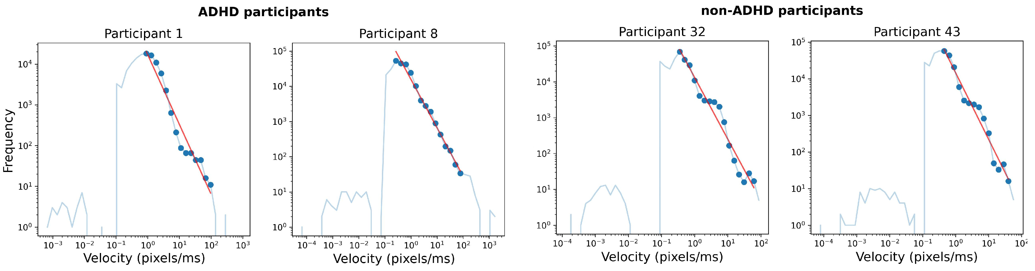
Figure 2.
Probability density for the distribution of the first statistical moments of across participants: mean (top left), standard deviation (top right), skewness (bottom left) and the kurtosis (bottom right).
Figure 2.
Probability density for the distribution of the first statistical moments of across participants: mean (top left), standard deviation (top right), skewness (bottom left) and the kurtosis (bottom right).
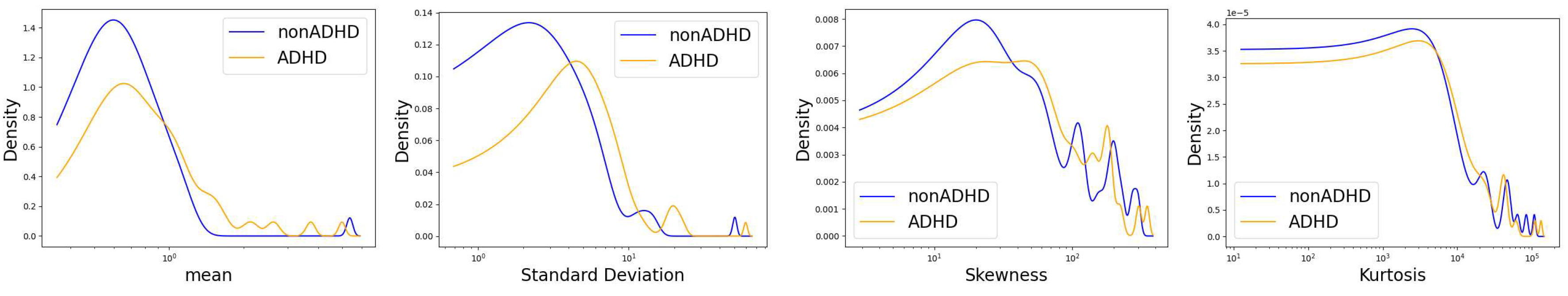
Figure 3.
Representation of the MSD as a function of the time window . The line in green represents the best quadratic fit to the data points, while the red one represents the best We observe that, on a log-log plot, the empirically estimated points fall along a straight line, which corroborates the relation .
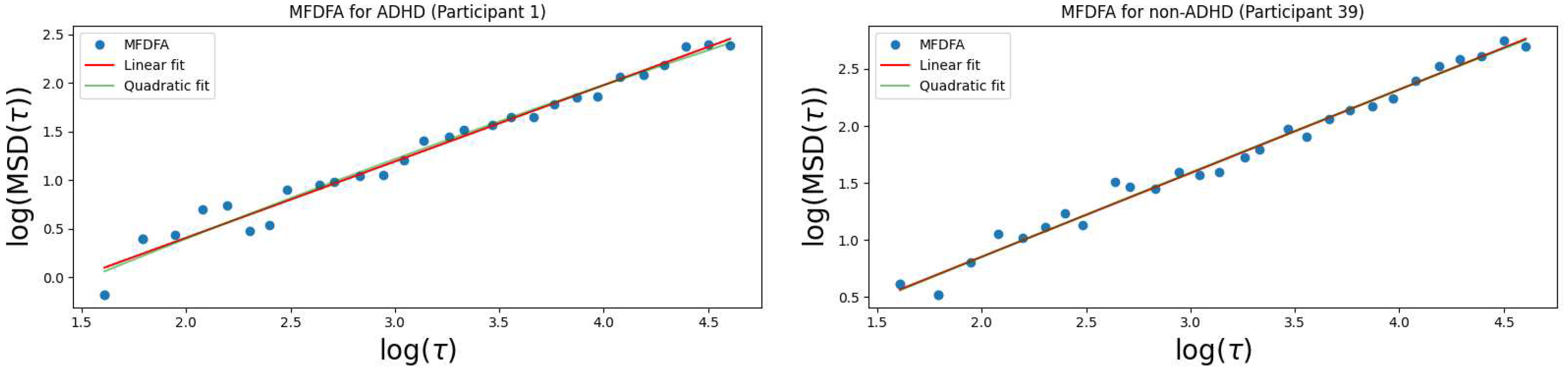
Figure 4.
Probability density of the R-square for the straight line fit on the log-log plot of the PDF decay, by virtue of which is estimated (left). On the right it is shown the coefficient of determination corresponding to the straight line fit on the MFDFA.
Figure 4.
Probability density of the R-square for the straight line fit on the log-log plot of the PDF decay, by virtue of which is estimated (left). On the right it is shown the coefficient of determination corresponding to the straight line fit on the MFDFA.
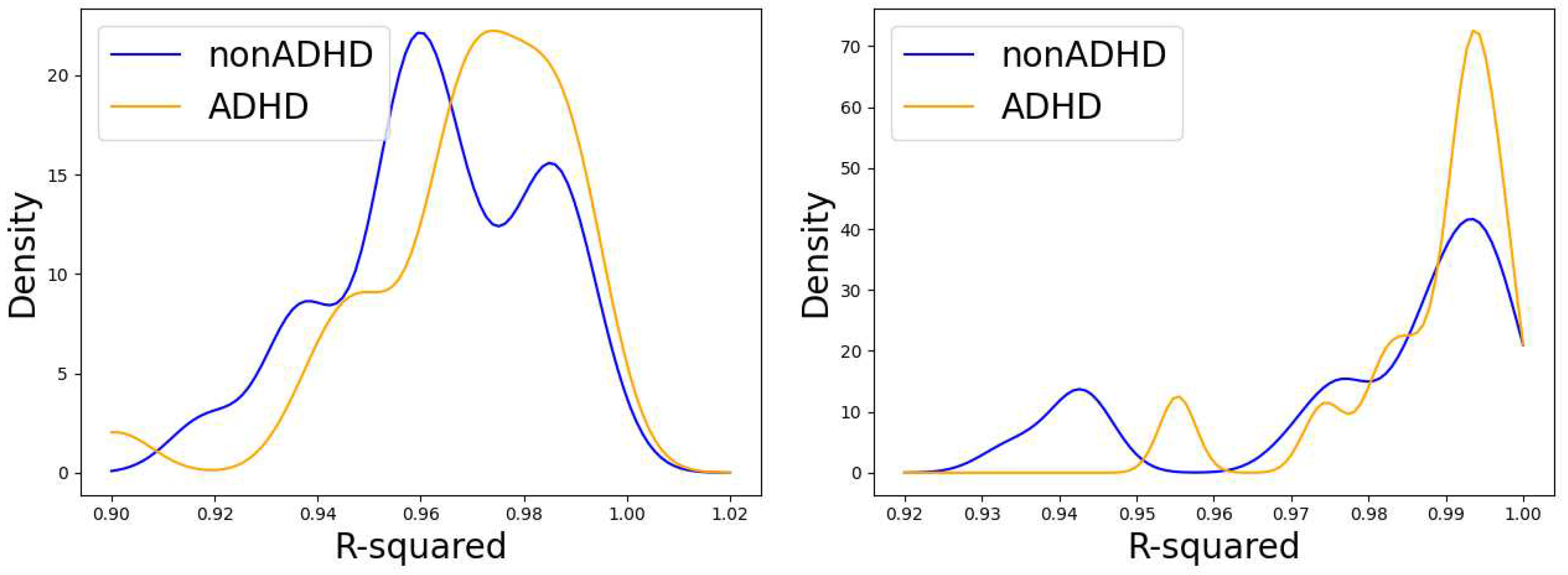
Figure 5.
Lévy exponent distributions for ADHD and normally developed children calculated via the increment’s pdf (left) and via the MFDFA method (right). A Mann-Whitney U statistical test confirms that the difference in medians is significant, with a p-value around (pdf estimation), (MFDFA estimation).


Table 1.
Accuracy values for different models using SKF and LOOC CV strategies.
| Method | Logistic | SVC | Decision | Random |
|---|---|---|---|---|
| Regression | Tree | Forest | ||
| SKF (k = 5) | 0.724 | 0.540 | 0.611 | 0.680 |
| LOOC | 0.724 | 0.540 | 0.596 | 0.724 |
Table 2.
Left - confusion matrix of the benchmark model with accuracy of , precision of , specificity of and recall . On the right we have the confusion matrix including the benchmark parameters as well as the Lévy exponent , yielding an accuracy of , precision of , specificity of and recall of .
Table 2.
Left - confusion matrix of the benchmark model with accuracy of , precision of , specificity of and recall . On the right we have the confusion matrix including the benchmark parameters as well as the Lévy exponent , yielding an accuracy of , precision of , specificity of and recall of .
 |
Disclaimer/Publisher’s Note: The statements, opinions and data contained in all publications are solely those of the individual author(s) and contributor(s) and not of MDPI and/or the editor(s). MDPI and/or the editor(s) disclaim responsibility for any injury to people or property resulting from any ideas, methods, instructions or products referred to in the content. |
© 2024 by the authors. Licensee MDPI, Basel, Switzerland. This article is an open access article distributed under the terms and conditions of the Creative Commons Attribution (CC BY) license (http://creativecommons.org/licenses/by/4.0/).
Copyright: This open access article is published under a Creative Commons CC BY 4.0 license, which permit the free download, distribution, and reuse, provided that the author and preprint are cited in any reuse.


