Research on Deployment Process Dynamics and Vibration for Replaceable Interface Mast

Preprint

Article

Research on Deployment Process Dynamics and Vibration for Replaceable Interface Mast

Altmetrics

Downloads

Views

Comments

A peer-reviewed article of this preprint also exists.

This version is not peer-reviewed

Submitted:

16 January 2024

Posted:

16 January 2024

You are already at the latest version

Alerts

Abstract

This paper studied the dynamic characteristics of the deployment process of the replaceable interface mast and the vibration generated at the end of the mast. The interface is discretized by the absolute nodal coordinate thin shell element with gradient reduction, and the three-dimensional motion of the reconfigurable rigid body module is described by the natural coordinate method. The dynamic equations of the interface and the reconfigurable module without external constraints are established by the principle of virtual work. Finally, the dynamic models of each part are assembled into the dynamic model of the mast system deployment process through the system constraint equation. According to the established dynamic model of the mast system deployment process, the dynamic behavior changes of the replaceable interface mast are analyzed. At the same time, the differences in the deployment behavior of the replaceable interface mast under different system configuration schemes, flexible interface geometric parameters, and different driving laws are studied and compared. It provides guidance for the scheme configuration of the mast system, the structural design of the interface, and the deployment motion planning of the mast. According to the physical prototype and the assembly of the mast system model, the deployment process of the replaceable interface mast is experimentally analyzed. It shows that the established dynamic model of the mast system can correctly analyze the dynamic characteristics of the deployment behavior of the replaceable interface mast, which provides a reference for the design and behavior analysis of the mast system.

Keywords:

Subject: Engineering - Aerospace Engineering

1. Introduction

The interplanetary rover mast is the mounting and support platform for highly sophisticated equipment such as navigation topography cameras and multispectral cameras on the rover [1]. In the space field, the research direction of modular spacecraft and on-orbit replacement has received a lot of attention for its high maintainability, so on-orbit replacement can be applied to the rover mast to extend its service time in orbit. One of the key technologies of the modular spacecraft is the fast docking between the modules [2,3,4,5,6,7]. Most of the studies have focused on the analysis of the dynamics of the docking mechanism during the docking process, but less on the influence of the docking mechanism on the dynamics of the completed system after the docking. Therefore, it is necessary to analyze the behavior of the mast end during deployment and to compare the dynamic behavior of the mast under different module configurations, different interface geometry parameters, and different deployment joint drive laws, to provide a basis for the structural and drive design of the replaceable interface mast. Fewer studies exist on the dynamical orientation of rover masts. In 2008, Li, Gao [8] et al. used Lagrangian equations combined with the Newton-Euler method to model the dynamics of the lunar rover mast during unfolding, however, the flexibility of the mast was not considered in the model developed. In 2015, Liu [9] et al. designed a new mast-locking mechanism and modeled the dynamics of each joint. The position error of the mast end and the repeatability accuracy were analyzed but the vibration deformation of the mast was also not considered. In 2017, Bindi You and Pei-Bo Hao [10] investigated the nonlinear dynamics characteristics of the mast deployment process of a laminated composite rover considering deformation, and gave the effect of the change of the laminated material's own parameters on the mast dynamics performance, but did not analyze the mast end dynamics performance influenced by the motion of the deployment joints.

The study of spacecraft dynamics with flexible accessories, such as spaceborne antennas and space manipulators, can also provide a certain reference for the study in this paper [11,12,13,14,15]. The multi-body system is divided into multi-rigid body system and multi-flexible body system, the development of multi-rigid body dynamics theory has become mature today, and the multi-flexible body system is the majority in practical problems, and the theoretical method of multi-flexible body dynamics can be mainly divided into floating coordinate system method and absolute node coordinate method [16,17,18,19]. To establish the dynamic model of a rigid-flexible multi-body system, it is necessary to describe the rigid body motion and the deformation motion of the flexible body separately [20,21,22,23,24]. In this paper, the dynamics model of the replaceable interface mast system will be established to analyze the end nonlinear behavior of the mast deployment process.

The remaining parts of the paper are presented as follows: In Section 2, the materials and methods we selected are introduced. In Section 3, the effect of nonlinear parameters on mast deployment is analyzed. In Section 4, the main conclusions are summarized.

2. Materials and Methods

In dealing with the replaceable interface mast, the reconfigurable modules within the mast are considered rigid bodies. As shown in Figure 1, two fixed points, p and q, and two unit vectors, u and v, are used to establish a natural coordinate system, x-y-z, on the rigid module.

Let Vr represent the volume of the reconfigurable rigid body module and ρ represents its density. The expression for the kinetic energy of the reconfigurable module can be calculated by Eq.1.

T = \frac{1}{2} (\int_{V_{r}} ρ {(A {\dot{q}}_{r})}^{T} A {\dot{q}}_{r} d V_{r}) = \frac{1}{2} {\dot{q}}_{r}^{T} M {\dot{q}}_{r}

(1)

Where Vr is the Volume of reconfigurable modules, M is the quality matrix of the reconfigurable module,

M = \int_{V_{r}} ρ A^{T} Ad V_{r}

; A is the shape functions of the rigid body module,

q_{r}

is a generalized coordinate system,

r

is a position vector in the global coordinate system.

The virtual work of inertial forces for reconfigurable modules can be calculated by Eq.2.

δ W_{g r} = - \int_{v_{r}} ρ δ r^{T} \ddot{r} d V_{r} = - δ {q_{r}}^{T} (\int_{v_{r}} ρ A^{T} A d V_{r}) {\ddot{q}}_{r} = - δ {q_{r}}^{T} M {\ddot{q}}_{r}

(2)

The external virtual work of the reconfigurable module can be written as Eq.3.

δ W_{e r} = - (δ {q_{r}}^{T} Q_{F} + δ {q_{r}}^{T} Q_{M})

(3)

In Eq.3, QF and QM respectively represent the generalized force columns of external force and external moment in the natural coordinate system. The virtual work done by the force F acting at any point N on the rigid body module can be expressed as Eq.4.

δ W_{F} = δ {r_{N}}^{T} F = δ {q_{r}}^{T} {A_{N}}^{T} F = δ {q_{r}}^{T} Q_{F}

(4)

Where A_N is the shape function corresponding to point N.

The virtual work of internal forces in the rigid body module is zero, hence, we can infer from the principle of virtual work that:

- δ {q_{r}}^{T} M {\ddot{q}}_{r} + (δ {q_{r}}^{T} Q_{F} + δ {q_{r}}^{T} Q_{M}) = - δ {q_{r}}^{T} (M {\ddot{q}}_{r} - Q_{F} - Q_{M}) = 0

(5)

Where

Q_{F}

is the generalized force due to external forces,

Q_{M}

is the generalized force corresponding to the moment M.

Establish the intrinsic constraint equations for the reconfigurable module in the natural coordinate system as Eq.6.

Φ (q_{r}, t) = 0

(6)

The dynamic equations for the reconfigurable rigid body module in the absence of external constraints can be obtained in Eq.7.

{\begin{matrix} M {\ddot{q}}_{r} = Q_{r} \\ Φ (q_{r}, t) = 0 \end{matrix}

(7)

Where

Q_{r} = Q_{F} + Q_{M}

The interface on the mast of the replaceable interface can be equivalently modeled as a cylindrical shell. The shell used in this paper has a thickness of h=2mm and a mid-surface radius of R=41mm, thus the interface can be represented by thin shell elements. The schematic diagram of the shell element deformation is shown in Figure 2.

The present study employs the gradient-reduced ANCF thin shell element [19] to discretize the finite element of the flexible interface's equivalent cylindrical shell model. The deformation along the thickness of the thin shell is neglected, and the overall deformation of the shell element is described through the stretching and shearing deformations on the mid-surface of the cylindrical shell element, as well as the bending deformation of the element.

2.1. Description of the movement of the shell unit

The nodal coordinates of the shell element, denoted as "e," are composed of the position coordinates and gradient coordinates of four points A, B, C, and D on the neutral surface. The nodal coordinates of each point can be expressed as Eq.8.

e_{i} = [\begin{matrix} r_{i} & \frac{\partial r_{i}}{\partial X} & \frac{\partial r_{i}}{\partial Y} \end{matrix}]

(8)

The first term in the expression represents the position coordinate array, while the second to the third terms represent the gradient coordinate array. Here, i represents the points A, B, C, and D, and the specific expressions for each term are as Eq.9.

{\begin{matrix} r_{i} = [\begin{matrix} r_{i, x} & r_{i, y} & r_{i, z} \end{matrix}] \\ \frac{\partial r_{i}}{\partial X} = [\begin{matrix} \frac{\partial r_{i, x}}{\partial X} & \frac{\partial r_{i, y}}{\partial X} & \frac{\partial r_{i, z}}{\partial X} \end{matrix}] \\ \frac{\partial r_{i}}{\partial Y} = [\begin{matrix} \frac{\partial r_{i, x}}{\partial Y} & \frac{\partial r_{i, y}}{\partial Y} & \frac{\partial r_{i, z}}{\partial Y} \end{matrix}] \end{matrix}

(9)

Therefore, the expression for the nodal coordinates of the element is as Eq.10.

e = [\begin{matrix} e_{A} & e_{B} & e_{C} & e_{D} \end{matrix}]

(10)

The position vector of any point Q on the neutral surface of the shell element in the global coordinate system is given by Eq.11.

r^{mid} = S (α, β) e

(11)

In the expression, S represents the shape function of the shell element. The expression for S is Eq.12.

S = [\begin{array}{l} S_{1} I_{3} & S_{2} I_{3} & \dots & S_{12} I_{3} \end{array}]

(12)

In the Eq.12. I₃ denotes the third-order identity matrix.

Therefore, the expressions for the velocity and acceleration of any point on the shell element can be obtained from the equation in Eq.13.

{\dot{r}}^{mid} = S (α, β) \dot{e} ， {\ddot{r}}^{mid} = S (α, β) \ddot{e}

(13)

2.2. Deformation modeling of shell units

As shown in Figure 2 and Figure 3, the schematic diagram represents a surface within the shell element, with the global coordinate system denoted as X-Y-Z and the α-β-γ system representing the curvilinear coordinates on the surface of the shell element.

The g10-g20-n0 and e10-e20-n0 correspond to the local curvilinear coordinate system and the Cartesian coordinate system on the shell element, respectively.

The vector of microsegments between two adjacent points Q and P on the midplane before and after the deformation can be written as Eq.14.

{\begin{cases} {(d s^{0})}^{2} = {(d r_{mid}^{0})}^{T} \cdot d r_{mid}^{0} = [\begin{array}{l} d α & d β \end{array}] [\begin{array}{l} {(g_{x}^{0})}^{T} g_{x}^{0} & {(g_{x}^{0})}^{T} g_{y}^{0} \\ {(g_{y}^{0})}^{T} g_{x}^{0} & {(g_{y}^{0})}^{T} g_{y}^{0} \end{array}] [\begin{array}{l} d α \\ d β \end{array}] \\ {(d s)}^{2} = {(d r_{mid})}^{T} \cdot d r_{mid} = [\begin{array}{l} d α & d β \end{array}] [\begin{array}{l} {g_{x}}^{T} g_{x} & {g_{x}}^{T} g_{y} \\ {g_{y}}^{T} g_{x} & {g_{y}}^{T} g_{y} \end{array}] [\begin{array}{l} d α \\ d β \end{array}] \end{cases}

(14)

The definition of the basis vectors for two sets of local coordinate systems on the mid-surface is as Eq.15.

{\begin{matrix} g_{x} = \frac{\partial r^{mid}}{\partial α} 、 g_{y} = \frac{\partial r^{mid}}{\partial β} 、 n = \frac{g_{x} \times g_{y}}{{‖ g_{x} \times g_{y} ‖}_{2}} \\ e_{x} = \frac{g_{x}}{{‖ g_{x} ‖}_{2}} 、 e_{z} = n 、 e_{y} = e_{z} \times e_{x} \end{matrix}

(15)

Coordinate transformation yields can be expressed as Eq.16.

[\begin{matrix} d α \\ d β \end{matrix}] = {[\begin{matrix} g_{x} e_{x} & g_{y} e_{x} \\ g_{x} e_{y} & g_{y} e_{y} \end{matrix}]}^{- T} [\begin{matrix} d x_{0} \\ d y_{0} \end{matrix}] = [\begin{matrix} \frac{1}{a} & - \frac{\cot (θ)}{a} \\ 0 & \frac{\csc (θ)}{b} \end{matrix}] [\begin{matrix} d x_{0} \\ d y_{0} \end{matrix}] = T_{θ} d X_{0}

(16)

Here, T_θ represents the transformation matrix from the Cartesian coordinate system to the curvilinear coordinate system, where θ denotes the angle between the coordinate axes of the curvilinear coordinate system.

The formula for calculating the Lagrange strain tensor can be derived from continuum mechanics as Eq.17.

{(d s)}^{2} - {(d s_{0})}^{2} = 2 d X_{0} ε d X_{0}

(17)

The expression for the mid-surface Lagrange strain tensor is obtained as Eq.18.

ε_{mid} = \frac{1}{2} T_{θ}^{T} ([\begin{array}{l} {g_{x}}^{T} g_{x} - {(g_{x}^{0})}^{T} g_{x}^{0} & {g_{x}}^{T} g_{y} - {(g_{x}^{0})}^{T} g_{y}^{0} \\ {g_{y}}^{T} g_{x} - {(g_{y}^{0})}^{T} g_{x}^{0} & {g_{y}}^{T} g_{y} - {(g_{y}^{0})}^{T} g_{y}^{0} \end{array}]) T_{θ} = [\begin{array}{l} ε_{11} & ε_{12} \\ ε_{21} & ε_{22} \end{array}]

(18)

Since ε_mid has symmetry, ε_mid can be rewritten as Eq.19.

ε_{mid} = {[ε_{11} ε_{22} 2 ε_{12}]}^{T}

(19)

From Figure 2-1, the position vector of any point Qʹ on the external surface of the shell unit can be expressed as Eq.20.

r = r_{mid} (α, β) + z n (α, β)

(20)

Then the basis vector of the surface coordinate system at point Qʹ can be calculated by Eq.21.

{\begin{array}{l} {g_{x}}^{'} = \frac{\partial r_{mid} (α, β)}{\partial α} + z \frac{\partial n (α, β)}{\partial α} \\ {g_{y}}^{'} = \frac{\partial r_{mid} (α, β)}{\partial β} + z \frac{\partial n (α, β)}{\partial β} \end{array}

(21)

Similarly, the length of the micro-segment arc between two adjacent points Qʹ and Pʹ on the external surface before and after the deformation can be obtained by Eq.22.

{\begin{cases} d {({s_{0}}^{'})}^{2} = [\begin{array}{l} d α & d β \end{array}] [\begin{array}{l} {({g_{x}}^{'})}_{0}^{T} {({g_{x}}^{'})}_{0} & {({g_{x}}^{'})}_{0}^{T} {({g_{y}}^{'})}_{0} \\ {({g_{y}}^{'})}_{0}^{T} {({g_{x}}^{'})}_{0} & {({g_{y}}^{'})}_{0}^{T} {({g_{y}}^{'})}_{0} \end{array}] [\begin{array}{l} d α \\ d β \end{array}] \\ d {(s^{'})}^{2} = [\begin{array}{l} d α & d β \end{array}] [\begin{matrix} {({g^{'}}_{x})}^{T} {g^{'}}_{x} & {({g^{'}}_{x})}^{T} {g^{'}}_{y} \\ {({g^{'}}_{y})}^{T} {g^{'}}_{x} & {({g^{'}}_{y})}^{T} {g^{'}}_{y} \end{matrix}] [\begin{array}{l} d α \\ d β \end{array}] \end{cases}

(22)

The Lagrange strain tensor for the shell element can be calculated by Eq.23.

ε \approx ε_{mid} + ε_{b} = \frac{1}{2} {T_{θ}}^{T} [\begin{matrix} {({g_{x}}^{'})}^{T} {g_{x}}^{'} - {({g_{x}}^{'})}_{0}^{T} {({g_{x}}^{'})}_{0} & {({g_{x}}^{'})}^{T} {g_{y}}^{'} - {({g_{x}}^{'})}_{0}^{T} {({g_{y}}^{'})}_{0} \\ {({g_{y}}^{'})}^{T} {g_{x}}^{'} - {({g_{y}}^{'})}_{0}^{T} {({g_{x}}^{'})}_{0} & {({g_{y}}^{'})}^{T} {g_{y}}^{'} - {({g_{y}}^{'})}_{0}^{T} {({g_{y}}^{'})}_{0} \end{matrix}] T_{θ}

(23)

Where

ε_{b}

is unit bending strain.

By neglecting higher-order terms in z, we obtain Eq.24. and Eq.25.

ε_{b} = - z A^{T} (l - l_{0}) A

(24)

{\begin{array}{l} l = [\begin{array}{l} {(\frac{\partial^{2} r_{mid}}{\partial α^{2}})}^{T} \cdot n & {(\frac{\partial^{2} r_{mid}}{\partial α \partial β})}^{T} \cdot n \\ {(\frac{\partial^{2} r_{mid}}{\partial β \partial α})}^{T} \cdot n & {(\frac{\partial^{2} r_{mid}}{\partial β^{2}})}^{T} \cdot n \end{array}] = [\begin{array}{l} l_{11} & l_{12} \\ l_{12} & l_{22} \end{array}] \\ l_{0} = [\begin{matrix} {(\frac{\partial^{2} r_{mid}^{0}}{\partial α^{2}})}^{T} \cdot n & {(\frac{\partial^{2} r_{mid}^{0}}{\partial α \partial β})}^{T} \cdot n \\ {(\frac{\partial^{2} r_{mid}^{0}}{\partial β \partial α})}^{T} \cdot n & {(\frac{\partial^{2} r_{mid}^{0}}{\partial β^{2}})}^{T} \cdot n \end{matrix}] = [\begin{array}{l} l_{11}^{0} & l_{12}^{0} \\ l_{21}^{0} & l_{22}^{0} \end{array}] \end{array}

(25)

2.3. Flexible interface dynamics model

Let the volume of the shell unit be Ve, and then the virtual work of the inertial force on the shell unit can be calculated by Eq.26.

δ W_{g e} = - \int_{V_{e}} ρ {\ddot{r}}^{T} δ r d V_{e} = - {\ddot{e}}^{T} (\int_{V_{e}} ρ S^{T} S d V_{e}) δ \dot{e} = - {\ddot{e}}^{T} M_{e} δ e

(26)

Where

M_{e} = \int_{V_{e}} ρ S^{T} S d V_{e}

is the mass matrix of the shell unit.

Therefore, the virtual work of inertia force for the flexible interface can be calculated by Eq.27.

δ W_{g d} = - \sum_{j = 1}^{n} \int_{V_{e j}} ρ {\ddot{r}}^{T} δ r d V_{e j} = - {\ddot{q}}_{f}^{T} M_{f} δ q_{f}

(27)

Where n is the number of shell units after interface discretization; Ve is the volume of the i-th shell unit.

q_{f}

is The generalized coordinates of the interface that can be calculated by Eq.28.

\begin{matrix} q_{f} = {[{e_{1}}^{T} \dots {e_{i}}^{T} \dots {e_{n}}^{T}]}^{T} ， & M_{f} = \sum_{j = 1}^{n} {B_{j}}^{T} M_{e j} B_{j} \end{matrix}

(28)

where B_j is denoted as the boolean matrix corresponding to each shell cell.

As the deformation of the shell element is decomposed into the bending deformation of the shell element and the deformation on the mid-surface, the strain energy of the shell element can be decomposed into the bending strain energy (Ub) and the mid-surface deformation strain energy (Umid), with the following calculation formulas.

U_{b} = \frac{1}{2} \int_{V_{e}} {(ε_{b})}^{T} E ε_{b} d V_{e} = \frac{1}{2} {\int_{V_{e}} Φ}^{T} K^{T} E K Φ d V_{e}

(29)

U_{mid} = \frac{1}{2} \int_{V_{e}} {(ε_{mid})}^{T} E ε_{mid} d V_{e}

(30)

Where E is the third-order modulus of the elasticity matrix; K is the equivalent transformation matrix of the bending strain tensor.

\begin{array}{l} E = \frac{E}{1 - υ^{2}} [\begin{matrix} 1 & υ & 0 \\ υ & 1 & 0 \\ 0 & 0 & \frac{1 - υ}{2} \end{matrix}] \\ Φ = - z {[\begin{matrix} l_{11} - l_{11}^{0} & l_{22} - l_{22}^{0} & 2 l_{12} - 2 l_{12}^{0} \end{matrix}]}^{T} \\ K = [\begin{matrix} \frac{1}{a^{2}} & 0 & 0 \\ \frac{\cot^{2} (θ)}{a^{2}} & \frac{\csc^{2} (θ)}{b^{2}} & - \frac{\cot (θ) \csc (θ)}{a b} \\ - \frac{2 \cot (θ)}{a^{2}} & 0 & \frac{\csc (θ)}{a b} \end{matrix}] \end{array}

(31)

Where

υ

is Poisson's ratio.

The derivative of the strain energy for the generalized coordinates yields the elastic forces on the neutral surface.

F_{mid} = \frac{\partial U_{mid}}{\partial e} = \int_{V_{e}} {(\frac{\partial ε_{mid}}{\partial e^{T}})}^{T} E ε_{mid} d V_{e}

(32)

The bending strain energy is derived for the generalized coordinates to obtain the bending elastic force as Eq.33.

F_{b} = \frac{\partial U_{b}}{\partial e} = \int_{V_{e}} {(\frac{\partial ε_{b}}{\partial e^{T}})}^{T} E ε_{b} d V_{e} = {\int_{V_{e}} (\frac{\partial Φ}{\partial e^{T}})}^{T} K^{T} E K Φ d V_{e}

(33)

Then the shell unit elastic force is

F_{s e} = F_{mid} + F_{b}

, so the internal force virtual work of the shell unit is

δ W_{i e} = {F_{s e}}^{T} δ e

, and the internal force virtual work of the flexible interface can be calculated by Eq.34 and Eq.35.

δ W_{i d} = \sum_{j = 1}^{n} {F_{s e}}^{T} δ e = - {Q_{s}}^{T} δ q_{f}

(34)

Q_{s} = \sum_{i = 1}^{n} F_{e} B_{i}

(35)

Let the generalized force acting on the interface be Q_a, then its corresponding external virtual work can be calculated by Eq.36.

δ W_{e d} = {Q_{a}}^{T} δ q_{f}

(36)

Then, from the principle of virtual work, we can obtain the equation as Eq.37.

\begin{matrix} δ W_{g d} + δ W_{i d} + δ W_{e d} = - {\ddot{q}}_{f}^{T} M_{g} δ q_{f} - {Q_{s}}^{T} δ q_{f} + {Q_{a}}^{T} δ q_{f} \\ = {(M_{f} {\ddot{q}}_{f} - Q_{f})}^{T} δ q_{f} = 0 \end{matrix}

(37)

Where

Q_{f} = Q_{a} - Q_{s}

Then the kinetic equation of the flexible interface without external constraints can be expressed as Eq.36.

M_{f} {\ddot{q}}_{f} - Q_{f} = 0

(38)

2.4. Dynamics model of the mast deployment process with replaceable interface

The schematic diagram of the interchangeable interface mast system, known as the "three interfaces and four modules," is illustrated in Figure 3.

When deriving the dynamics equations for the expansion process of the interchangeable interface mast system, the following assumptions are made:

(1) The reconfigurable module is considered as a fixed constraint between the reconfigurable module and the flexible interface;

(2) The rotation constraint is between the reconfigurable module and the body of the rover (base);

(3) The mast deployment process does not consider the effect of gravity;

(4) The body of the rover is considered a rigid body, and the body of the rover is at rest when the mast is deployed.

After establishing the dynamic equations for each part separately, it is necessary to establish the dynamic equations of the mast system by simultaneously combining the dynamic models of each part through the system's constraint equations. The constraints of the mast system include the articulated constraints between the reconfigurable modules and the inspector body, the fixed constraints between the reconfigurable modules and the flexible interfaces, as well as the intrinsic constraints introduced when modeling the reconfigurable modules using NCF.

The reconfigurable modules, which are described by the NCF method to depict the motion of rigid bodies, possess 12 generalized coordinates. Consequently, it is necessary to impose 6 constraints, including the mutual orthogonality constraints between three basis vectors and the length constraints of the basis vectors. The expression for the constraint equations of the rigid body is as Eq.39.

Φ_{q_{r}} : {\begin{array}{l} ‖ r_{j} - r_{i} ‖ = d ， & u^{T} (r_{j} - r_{i}) = 0 \\ ‖ u ‖ = 1 ， & v^{T} (r_{j} - r_{i}) = 0 \\ ‖ v ‖ = 1 ， & u^{T} v = 0 \end{array}

(39)

Where d is the side length of the reconstructed module (m).

2.5. Fixed Constraints

The fixed constraint limits the position between the origin of the coordinate system on the shell unit and the nodes on the rigid module and the rotation of the interchangeable interface for the rigid module, as shown in Figure 4.

The gradient vector along the x-direction at the nodes A and B during the unfolding process is always perpendicular to the vector u. As Eq.40.

Φ_{f} : {\begin{array}{l} {‖ r_{A} - r_{j} ‖}_{2} = {‖ {\bar{r}}_{A j} ‖}_{2} \\ {‖ r_{B} - r_{j} ‖}_{2} = {‖ {\bar{r}}_{B j} ‖}_{2} \\ \frac{\partial r_{A}}{\partial x} \cdot u = 0 \\ \frac{\partial r_{B}}{\partial x} \cdot u = 0 \\ \frac{\partial r_{A}}{\partial x} \cdot v = 0 \\ \frac{\partial r_{B}}{\partial x} \cdot v = 0 \end{array}

(40)

Where

{‖{\bar{r}}_{A j}‖}_{2} 、 {‖{\bar{r}}_{B j}‖}_{2}

is the radius of the neutral surface of the interface.

2.6. Rotation constraints

The rotational constraints between the reconfigurable module and the base are illustrated in Figure 4-2. Here, the x-y-z axes represent the local coordinate system of the rigid body, while the X-Y-Z axes represent the global coordinate system. Thus, the center of mass of the rigid body module coincides with the origin of the global coordinate system. Additionally, during the rotation of the rigid body module, the ox and oy axes are always perpendicular to the OZ axis. Hence, the constraint equations can be expressed as Eq.41.

Φ_{R} : {\begin{array}{l} r_{c} = 0 \\ [\begin{matrix} 0 & 0 & 1 \end{matrix}] \cdot u = 0 \\ [\begin{matrix} 0 & 0 & 1 \end{matrix}] \cdot r_{j i} = 0 \end{array}

(41)

2.7. Mast system dynamics equation

For a system of replaceable interface masts with m flexible interfaces and n reconfigurable modules, the dynamical equations in the unfolding process can be expressed as Eq.41.

- \sum_{i = 1}^{n} δ {q_{r i}}^{T} (M_{r i} {\ddot{q}}_{r i} - Q_{r i}) + \sum_{j = 1}^{m} δ {q_{f j}}^{T} (M_{f j} {\ddot{q}}_{f j} - Q_{f j}) = 0

(42)

Let

q = {[q_{r 1} \dots q_{r n} q_{f 1} \dots q_{f m}]}^{T}

be the generalized coordinates of the total interchangeable interface mast system, then the above equation can be rewritten as Eq.43.

- δ q^{T} (M \ddot{q} - Q_{a}) = 0

(43)

M = d i a g \{M_{r 1} \dots M_{r n} M_{f 1} \dots M_{f m}\}

Q_{a} = d i a g \{Q_{r 1} \dots Q_{r n} Q_{f 1} \dots Q_{f m}\}

The replaceable interface mast system has a total of 1 rotational constraint and 2m fixed constraints, and the constraint equation of the mast system can be obtained by Eq.44.

Φ (q_{r}, q_{d}, t) = 0

(44)

Where

q_{d} = [q_{f 1} q_{f 2} \dots q_{f m}]

is the total generalized coordinate of the interface contained in the mast system.

The dynamical equations in matrix form during the unfolding of the mast system can be obtained by associating the Lagrange multiplier method. As Eq.45.

[\begin{matrix} M & Φ_{q}^{T} \\ Φ_{q} & 0 \end{matrix}] [\begin{matrix} \ddot{q} \\ λ \end{matrix}] = [\begin{matrix} Q_{a} \\ ψ \end{matrix}]

(45)

Where

Φ_{q}

the Jacobi matrix of the system constraint equations for the generalized coordinates of the system; λ is the Lagrange multiplier array.

The expression obtained as Eq.46. by taking the second-order derivative of the constraint equation

Φ (q_{r}, q_{d}, t)

for time and organizing.

\begin{array}{l} ψ = Φ_{q} \ddot{q} = - {(Φ_{q_{r}} {\dot{q}}_{r})}_{q_{r}} {\dot{q}}_{r} - {(Φ_{q_{r}} {\dot{q}}_{r})}_{q_{d}} {\dot{q}}_{f} - {(Φ_{q_{f}} {\dot{q}}_{d})}_{q_{d}} {\dot{q}}_{d} \\ - {(Φ_{q_{d}} {\dot{q}}_{d})}_{q_{r}} {\dot{q}}_{r} - 2 (Φ_{q_{r} t} {\dot{q}}_{r} + Φ_{q_{d} t} {\dot{q}}_{d}) - Φ_{t t} \end{array}

(46)

3. Analysis of the effect of nonlinear parameters on mast deployment

To provide a reference for the actual design and structural configuration of the replaceable mast, it is necessary to analyze the mast dynamic behavior in-depth under different configurations of structural solutions, interface radius of curvature, section thickness, and driving law factors. The schematic of the comparative analysis of mast system parameters is shown in Figure 5.

The trapezoidal velocity plan is chosen for unfolding the drive method of the joint due to its widely used, and the joint angular acceleration equation can be expressed as Eq.47.

ω = {\begin{array}{l} 150 t & , 0 \leq t \leq 0.1 \\ 0 & , 0.1 \leq t \leq 6 \\ - 150 t + 915 & , 6 \leq t \leq 6.1 \\ 0 & , 6.1 \leq t \end{array}

(47)

3.1. Non-linear effects of structural configuration

The three-mast combination schemes are shown in Figure 6. Scheme 1 is assembled by one flexible interface in series with two reconfigurable rigid modules. Scheme 2 uses two replaceable interfaces to connect three reconfigurable modules. The scheme is assembled by three replaceable interfaces and four reconfigurable modules.

The comparison of the angular acceleration at the end of the mast and the force at the deployment joint for different scenarios is shown in Figure 7 and Figure 8, where Scheme 3 has a large mass moment. Therefore, under the same velocity plan, the force at the deployment joint is the largest and the acceleration generated at the end is also the largest and lasts the longest.

3.2. Non-linear effect of different shell thickness

The mast model is selected as the replaceable interface mast in Scheme 3, and the interface shell thickness is set as δ=0.5mm, δ=1.0mm, and δ=1.5mm for three cases. The angular acceleration and the force at the unfolded joint for the three shell thicknesses are shown in Figure 9 and Figure 10.

Based on comparative analysis, it was observed that the attenuation of angular acceleration during the mast alignment process and residual vibration process is directly proportional to the shell thickness. As the shell thickness increases, the force at the deployment joint attenuates more rapidly, resulting in a shorter duration of angular acceleration vibrations.

The same configuration is carried out according to Scheme 3, and the inner diameter of the interface is set as d=85 mm, d=90 mm, and d=100 mm.

The absolute angular acceleration at the end of the mast and the change of force at the deployment joint are shown in Figure 11 and Figure 12. The results show that the interface in the replaceable mast should be designed with the system requirements in mind while appropriately expanding the inner diameter of the interface to improve the vibration and deformation resistance of the mast system.

3.3. Driving law non-linear influence

The unfolded joint angles are planned for cubic polynomial, quintuple polynomial, and pendulum motion laws. The initial conditions of motion are given as Eq.48.

{\begin{matrix} θ_{c} (0) = 0, {\dot{θ}}_{c} (0) = 0 \\ θ_{c} (t_{c}) = \frac{π}{2}, {\dot{θ}}_{c} (t_{c}) = 0 \end{matrix}, {\begin{matrix} θ_{q} (0) = 0, θ_{q} (t_{q}) = π / 2 \\ {\dot{θ}}_{q} (0) = 0, {\dot{θ}}_{q} (t_{q}) = 0 \\ {\ddot{θ}}_{q} (0) = 0, {\ddot{θ}}_{q} (t_{q}) = 0 \end{matrix}

(48)

Then the corresponding joint angle cubic and quintuple polynomial planning can be expressed as Eq.49.

\begin{array}{l} θ_{c} (t) = \frac{π}{2} - π {(\frac{t}{t_{c}})}^{3} + \frac{3 π}{2} {(\frac{t}{t_{c}})}^{2} \\ θ_{q} = 3 π {(\frac{t}{t_{q}})}^{5} - \frac{15 π}{2} {(\frac{t}{t_{q}})}^{4} + 5 π {(\frac{t}{t_{q}})}^{3} \end{array}

(49)

The equation for the law of motion of the joint angle pendulum [9] can be expressed as Eq.50.

θ_{b} (t) = \frac{π}{2} [\frac{t}{t_{b}} - \frac{1}{2 π} \sin (\frac{2 π t}{t_{b}})]

(50)

The absolute and relative angular accelerations at the endpoint of the mast under the three types of motion are shown in Figure 13 and Figure 14. The mast with the unfolding joint angle changing according to the cubic polynomial has the worst stability and the most violent vibration, and the sudden change in acceleration at the beginning and the end of the motion causes a large vibration in the angular acceleration with amplitudes of 23.24 deg/s² and 24.10 deg/s² respectively. The decay time of the angular acceleration is the longest under the law of motion.

3.4. Experimental analysis of replaceable mast deployment

The mast system is transformed from vertical to horizontal, a pulley is added to the mast system to change the sliding friction to rolling friction, and a triaxial accelerometer is mounted at the center point of the mast end of the interchangeable interface.

The experimental analysis of the unfolding process of the mast under different scheme configurations was carried out with a driving speed of 15 deg/s and a movement angle of 90deg for the unfolding joints.

The mast deployment experimental system and the schematic diagram of the gravity compensation scheme are shown in Figure 15 and Figure 16.

The acceleration comparison results of the endpoints of the mast under different scheme configurations are shown in Figure 17-1, Figure 17-2 and Figure 17-3.

The reconfigurable module used in the experiments is machined from resin material, so the simulation results need to be compared with those of interchangeable interface masts of the same material. At the same time, the triaxial acceleration sensor measures the linear acceleration along the tangential direction of the mast endpoint, while the simulation measures the angular acceleration signal at the mast endpoint. Therefore, the angular acceleration signal obtained from the simulation is first converted into linear acceleration and then compared with the experimental results.

The comparative analysis of experimental data has confirmed that the greater the number of interface configurations, the more pronounced the vibration of the mast system, as indicated by simulation results. Furthermore, during the abrupt change in motion state at the onset of movement, there was a high degree of conformity between the experimental and theoretical acceleration curves for all three scenarios, with similar acceleration oscillation amplitudes. Throughout the uniform deployment motion of the mast, the experimental acceleration curve consistently exhibited a certain degree of oscillation. Upon completion of the motion, the experimental curve took some time to stabilize compared to the theoretical results. This is primarily attributable to the incomplete compensation for the effects of gravity during the experimental process. Additionally, the inherent vibration of mechanical equipment such as motors and platforms, as well as the deformation of the reconfigurable module, also contributed to some extent to the observed discrepancies in the experimental results.

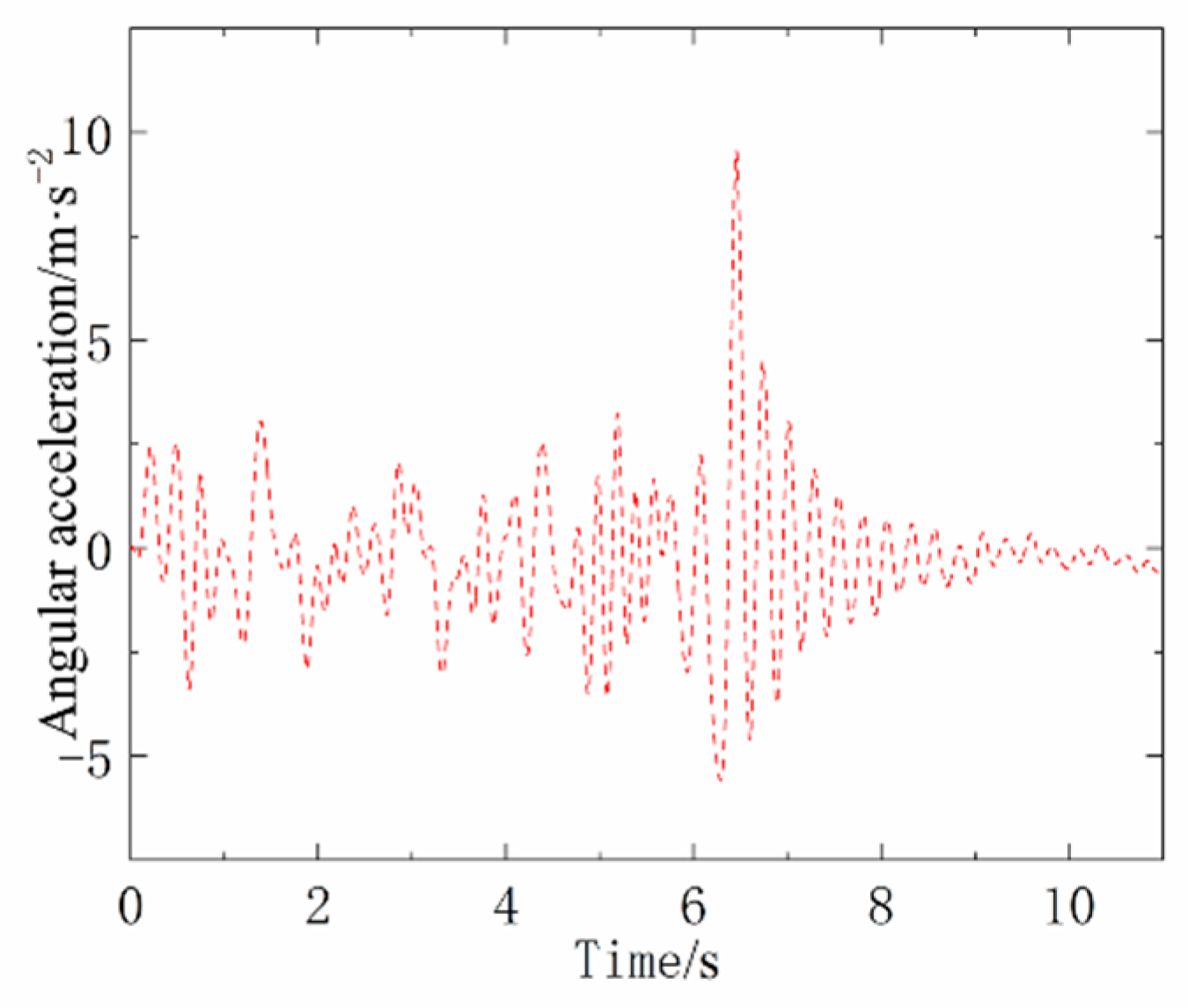
To verify the errors caused by the deformation of reconfigurable modules in the experiment, the flexible interface in Scheme 1 is now replaced by a functional prototype with a more rigid interface for analysis. A comparison of the end acceleration of Scheme 1 before and after the replacement of the interface function prototype is shown in Figure 18.

There are large vibrations in the acceleration during the entire unfolding of the mast. This is due to the flexible deformation of the reconfigurable module machined in the experiment leading to more intense vibration of the mast system.

4. Conclusion

In light of the limited redundancy and poor maintainability of conventional inspection mast systems, this paper combines the concepts of modular spacecraft and on-orbit replacement to propose the design concept of a redundant replaceable interface mast. Addressing the issue of system vibration caused by interface flexibility and its impact on the performance and operational quality of equipment mounted on the mast, the paper systematically investigates the deployment behavior and vibration suppression of a rigid-flexible coupled mast system. The research contributes valuable insights to the structural design, configuration planning, drive planning, and vibration control of replaceable interface masts.

The key achievements of this study include the following aspects:

(1) Establishment of a dynamic model for the deployment process of the replaceable interface mast system. Considering the characteristics of the rigid-flexible multibody system of the replaceable interface mast, the paper models two types of components in the system separately and establishes the dynamic model of the mast system by incorporating system constraint equations. The comparison of numerical simulation results of the mast system's dynamic equations with software calculations demonstrates the correctness and effectiveness of the rigid-flexible multibody mast system's dynamic model. This model holds significance for the dynamic modeling of complex systems involving multiple rigid and flexible bodies.

(2) Analysis of the dynamic behavior changes during the deployment process of the replaceable mast system, investigating the influence of different system configuration schemes, interface geometric parameters, and various deployment motion patterns on the mast system's deployment behavior. Despite the higher mass of the replaceable interface mast compared to a regular mast of the same length, the introduction of a high-stiffness reconfigurable module in the replaceable mast increases the overall stiffness, resulting in reduced vibration deformation at the mast's endpoint. The quantity of flexible interfaces and reconfigurable rigid body modules in the mast system directly correlates with more drastic force variations at the deployment joint and nonlinear amplification of endpoint vibrations. Thinner interface shell thickness weakens the resistance to deformation, leading to increased endpoint vibrations and slower attenuation rates. Enlarging the interface inner diameter increases the sectional moment of inertia, enhancing interface stiffness and accelerating the force attenuation at the deployment joint, resulting in decreased endpoint vibration. The use of harmonic motion planning minimizes mast vibration, underscoring the need to avoid sudden changes in angular acceleration and ensure a smooth acceleration profile to minimize vibrations. The theoretical model established considers and analyzes various nonlinear factors affecting the deployment behavior of the replaceable mast system, providing guidance for configuration, structural design, and drive planning of the mast.

(3) Conducted on-ground deployment experiments for the replaceable interface mast, validating the scientific validity of the dynamic theoretical model and the correctness of simulation results. Experimental results for different configuration schemes of the replaceable mast indicate that increasing the quantity of interfaces and reconfigurable modules intensifies mast vibrations.

While this paper presents significant contributions, areas for improvement have been identified for future research:

(1) In the establishment of the mast system's dynamic model, further research can be conducted to examine the variations in mast system deployment behavior when considering the flexibility of reconfigurable modules.

(2) Due to limitations in measurement equipment, the experiments verified only the acceleration of the mast's endpoint. Future research could extend the verification to include angular velocity at the endpoint and the torque at the deployment joint.

Author Contributions

T.L. conducted data extraction, performed the analyses, and wrote the article. J.W. conceived and designed the study, and applied for the funding which financially supported the study. All authors have read and agreed to the published version of the manuscript.

Funding

This work is supported by the National Natural Science Foundation of China under Grant No. 52075116.

Conflicts of Interest

The authors declare that they have no known competing financial interests or personal relationships that could have appeared to influence the work reported in this paper.

References

Warner N, Silverman M, Samuels J, et al. The Mars Science Laboratory Remote Sensing Mast: IEEE, 2016. [CrossRef]
Ren J, Kong N, Zhuang Y, et al. A review on the interfaces of orbital replacement unit: Great efforts for modular spacecraft[J]. Proceedings of the Institution of Mechanical Engineers, Part G: Journal of Aerospace Engineering, 2021,235(14): 1941-1967. [CrossRef]
Rossetti D, Keer B, Panek J, et al. Spacecraft modularity for serviceable satellites, 2015. [CrossRef]
Ren J, Kong N, Zhuang Y, et al. A review on the interfaces of orbital replacement unit: Great efforts for modular spacecraft[J]. Proceedings of the Institution of Mechanical Engineers, Part G: Journal of Aerospace Engineering, 2021,235(14): 1941-1967. [CrossRef]
The Rover's "Neck and Head"[EB/OL]. [2022-5-27]. https://mars.nasa.gov/mer/ mission/rover/neck-and-head/.
Mars Curiosity: Facts and Information[EB/OL]. [2022-5-27]. https://www.spac e.com/17963-mars-curiosity.html.
China's Chang'e-3 lander and Jade Rabbit rover land on moon - SlashGear [EB/OL]. [2022-5-27]. https://www.slashgear.com/chinas-change-3-lander-and-jade-rabbitrover-land-on-moon-14308846/.
Li H J, Gao H B, Deng Z Q. Design and analysis of the lunar rover mast mechanism[J]. Robot, 2008,30(1): 13-16.
Liu G, Liu Y, Zhang H, et al. The kapvik robotic mast: an innovative onboard robotic arm for planetary exploration rovers[J]. IEEE Robotics & Automation Magazine, 2015,22(1): 34-44. [CrossRef]
Hao P, You B, Sun Y, et al. Nonlinear dynamic analysis of deployment of laminated planetary rover mast: IEEE, 2017. [CrossRef]
Jonker B. A Finite Element Dynamic Analysis of Flexible Manipulators[J]. The International Journal of Robotics Research, 1990,9(4): 59-74. [CrossRef]
Modi V J, Mah H W, Misra A K. On the non-linear dynamics of a space platform based mobile flexible manipulator[J]. Acta Astronautica, 1994,32(6): 419-439. [CrossRef]
Li Q, Deng Z, Zhang K, et al. Unified modeling method for large space structures using absolute nodal coordinate[J]. AIAA Journal, 2018,56(10): 4146-4157. [CrossRef]
Nanos K, Papadopoulos E G. On the dynamics and control of flexible joint space manipulators[J]. Control Engineering Practice, 2015,45: 230-243. [CrossRef]
Meng D, She Y, Xu W, et al. Dynamic modeling and vibration characteristics analysis of flexible-link and flexible-joint space manipulator[J]. Multibody System Dynamics, 2018,43(4): 321-347. [CrossRef]
Shabana A A. Flexible multibody dynamics: review of past and recent developments[J]. Multibody system dynamics, 1997,1(2): 189-222. [CrossRef]
Dmitrochenko O N, Pogorelov D Y. Generalization of plate finite elements for absolute nodal coordinate formulation[J]. Multibody System Dynamics, 2003,10(1): 17-43. [CrossRef]
Sugiyama H, Koyama H, Yamashita H. Gradient deficient curved beam element using the absolute nodal coordinate formulation[J]. Journal of computational and nonlinear dynamics, 2010,5(2). [CrossRef]
Liu C, Tian Q, Hu H. New spatial curved beam and cylindrical shell elements of gradient-deficient Absolute Nodal Coordinate Formulation[J]. Nonlinear Dynamics, 2012,70(3): 1903-1918. [CrossRef]
García-Vallejo D, Escalona J L, Mayo J, et al. Describing Rigid-Flexible Multibody Systems Using Absolute Coordinates[J]. Nonlinear Dynamics, 2003,34(1): 75-94. [CrossRef]
Shabana A A. ANCF reference node for multibody system analysis[J]. Proceedings of the Institution of Mechanical Engineers, Part K: Journal of Multi-body Dynamics, 2014,229(1): 109-112. [CrossRef]
Wang Z, Tian Q, Hu H. Dynamics of spatial rigid–flexible multibody systems with uncertain interval parameters[J]. Nonlinear Dynamics, 2016,84(2): 527-548.
Li K, Tian Q, Shi J, et al. Assembly dynamics of a large space modular satellite antenna[J]. Mechanism and Machine Theory, 2019,142: 103601. [CrossRef]
Li Y, Wang C, Huang W. Dynamics analysis of planar rigid-flexible coupling deployable solar array system with multiple revolute clearance joints[J]. Mechanical Systems and Signal Processing, 2019,117: 188-209. [CrossRef]
Zhuang peng, Yao zhengqiu. Trajectory planning of suspended-cable parallel robot based on law of cycloidal motion [J]. J O U RN AL OF M AC HI N E DESI G, 2006(09): 21-24.

Figure 1. Description of the position of the rigid body module.

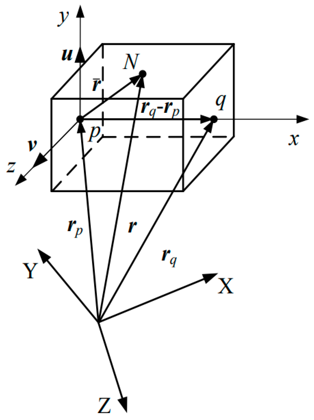
Figure 2. The schematic diagram of the shell element deformation.

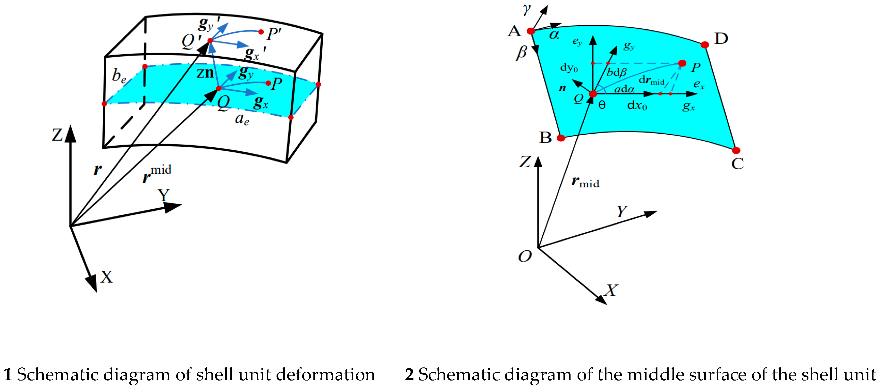
Figure 3. Schematic diagram of replaceable interface mast composition.

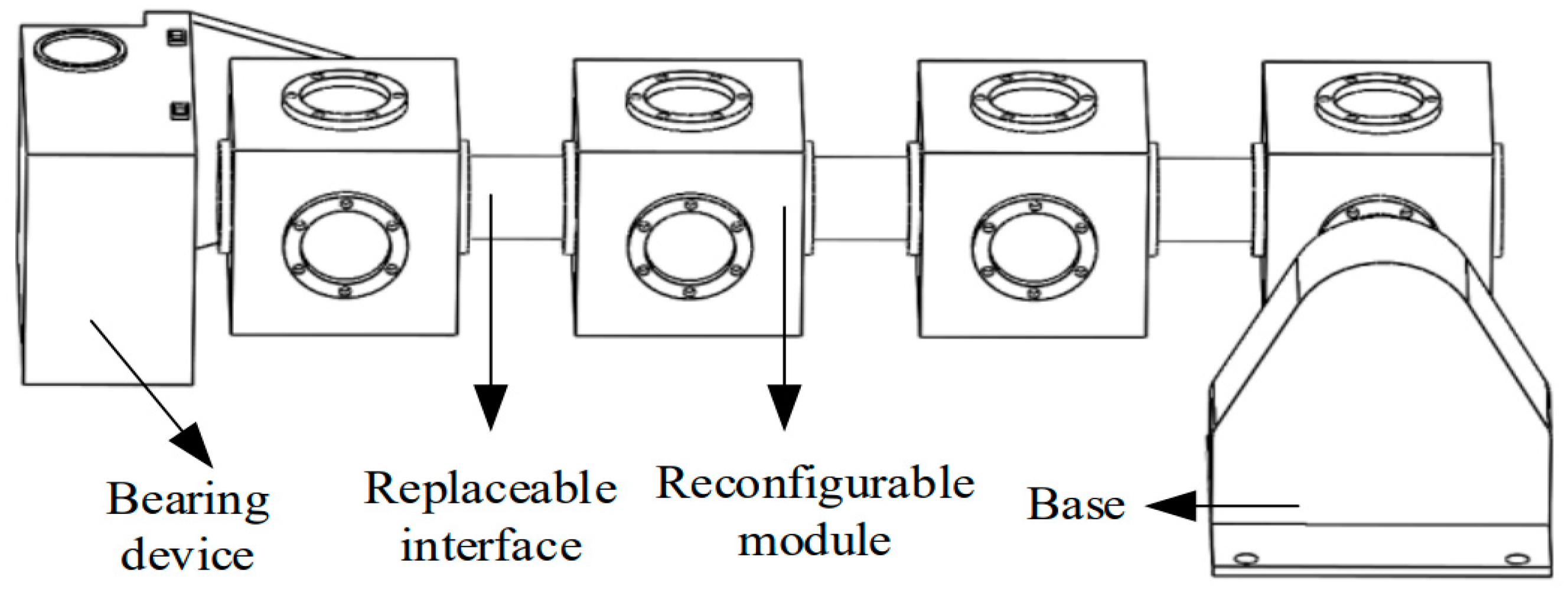
Figure 4. Schematic diagram of fixed constraint and rotational constraints.

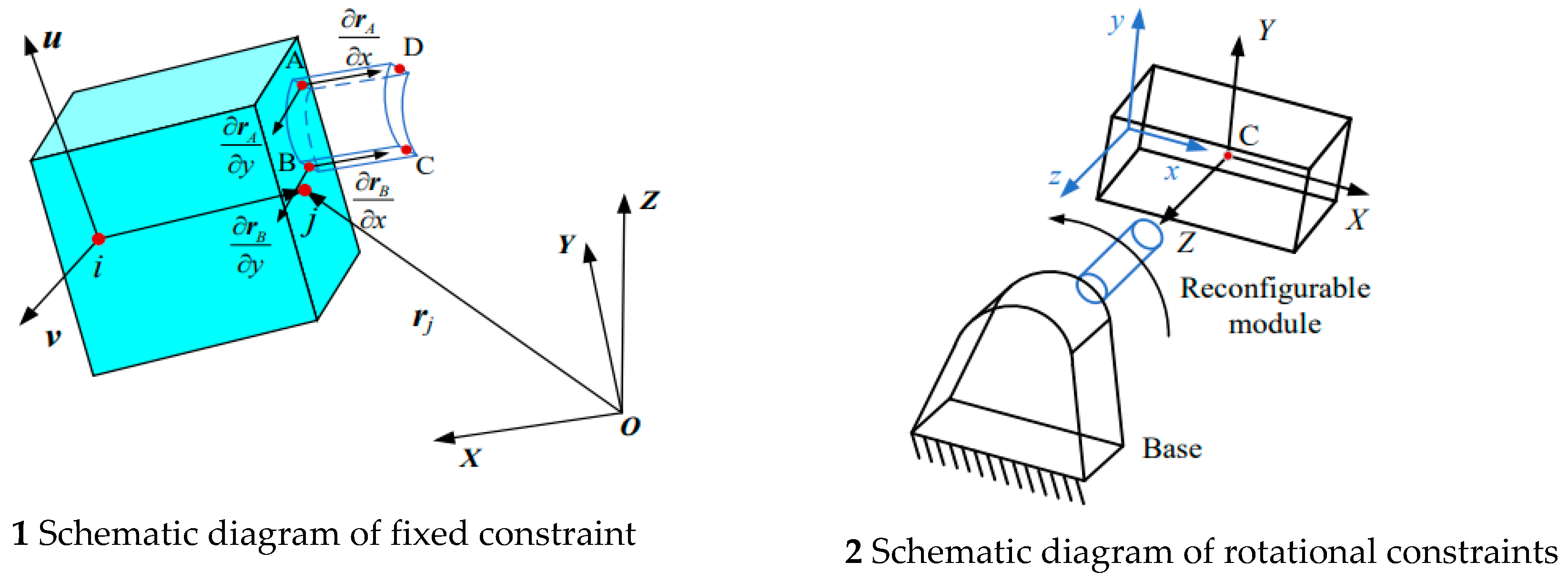
Figure 5. The schematic diagram of the comparative analysis of mast system parameters.

Figure 6. Schematic diagram of the structure of different combination schemes.

Figure 7. Absolute angular acceleration.

Figure 8. Force at the expansion joint.

Figure 9. Absolute angular acceleration.

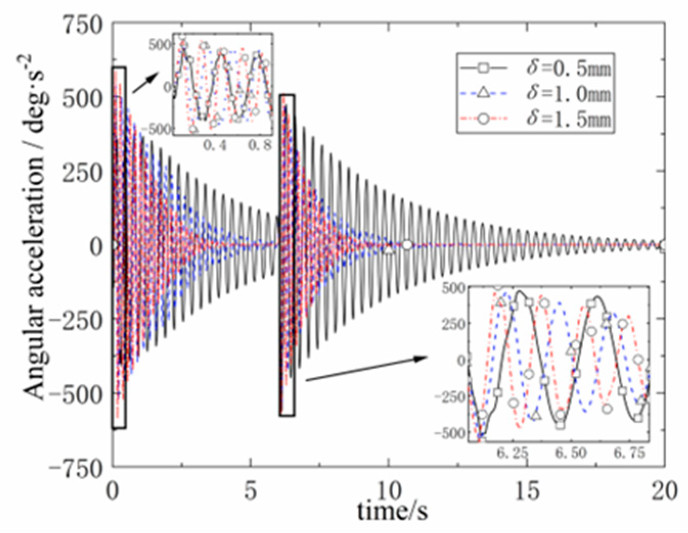
Figure 10. Expanding joint forces.

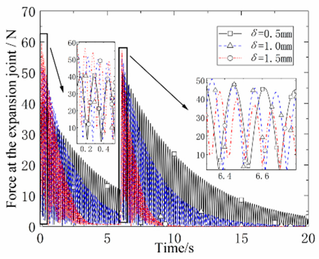
Figure 11. Absolute angular acceleration.

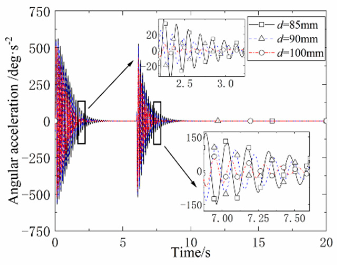
Figure 12. Force at the spread joint.

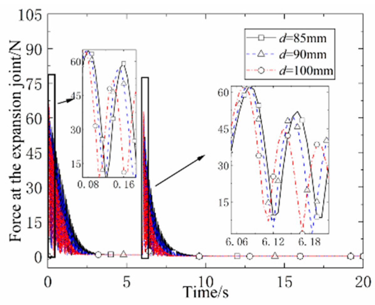
Figure 13. Absolute angular acceleration.

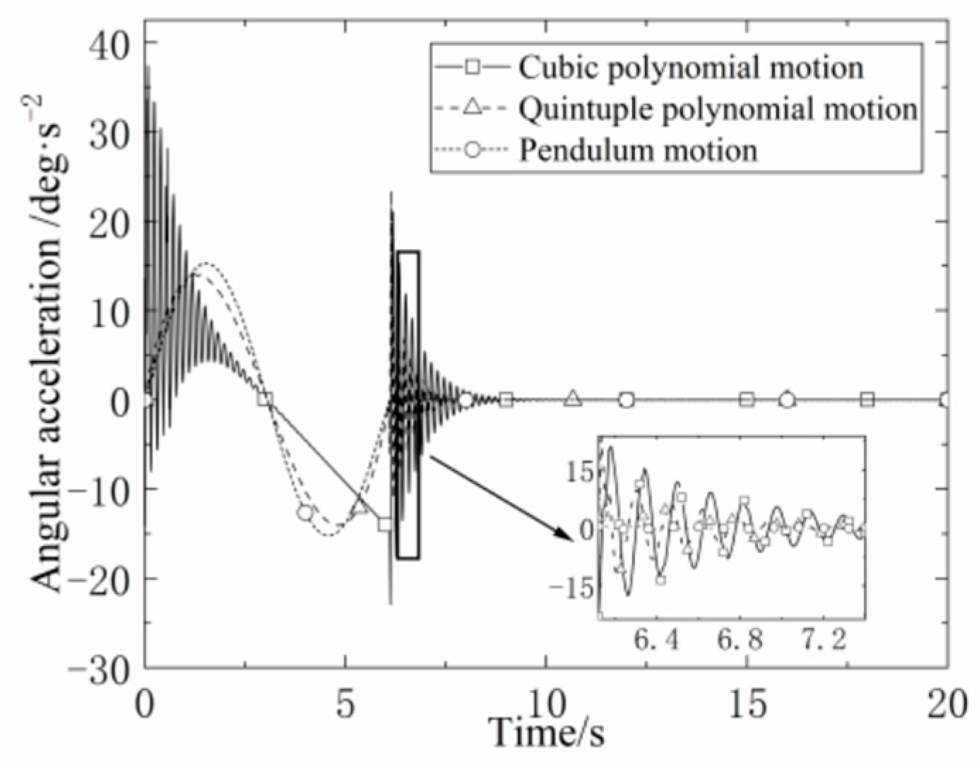
Figure 14. Relative angular acceleration.

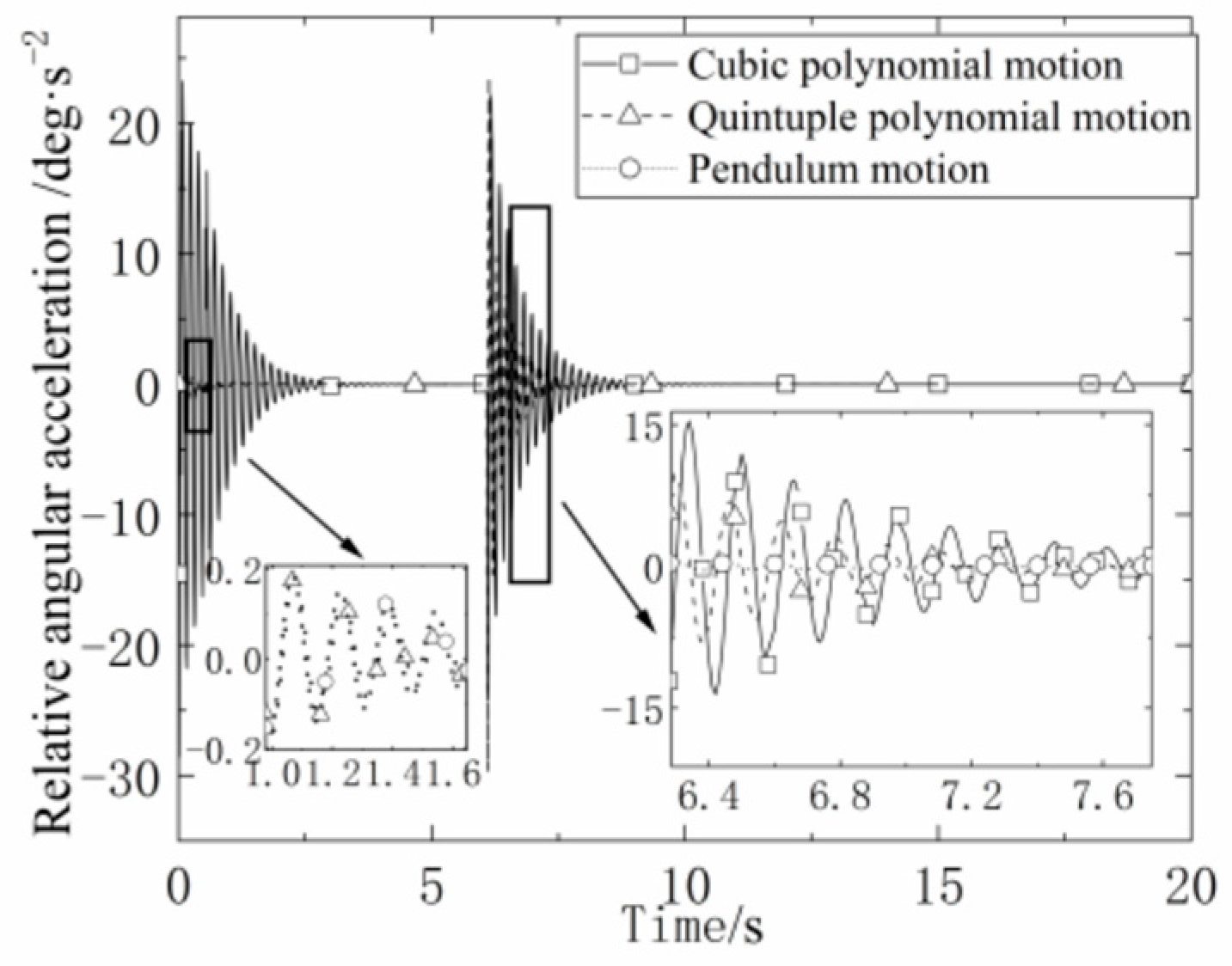
Figure 15. Mast deployment experimental system.

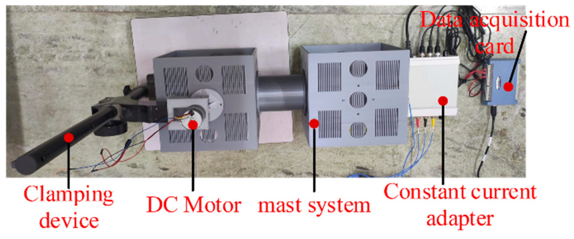
Figure 16. Schematic diagram of the gravity compensation scheme.

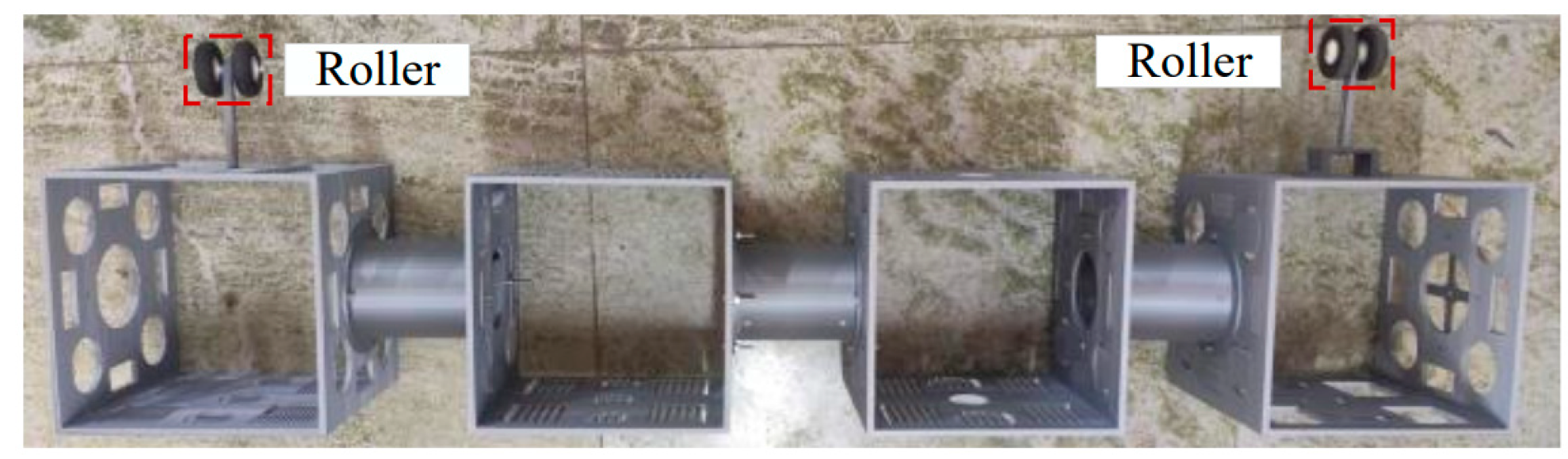
Figure 17. 1 Comparison of Experiment and Simulation of Scheme 1. 2 Comparison of Experiment and Simulation of Scheme 2. 3 Comparison of Experiment and Simulation for Scenario 3.

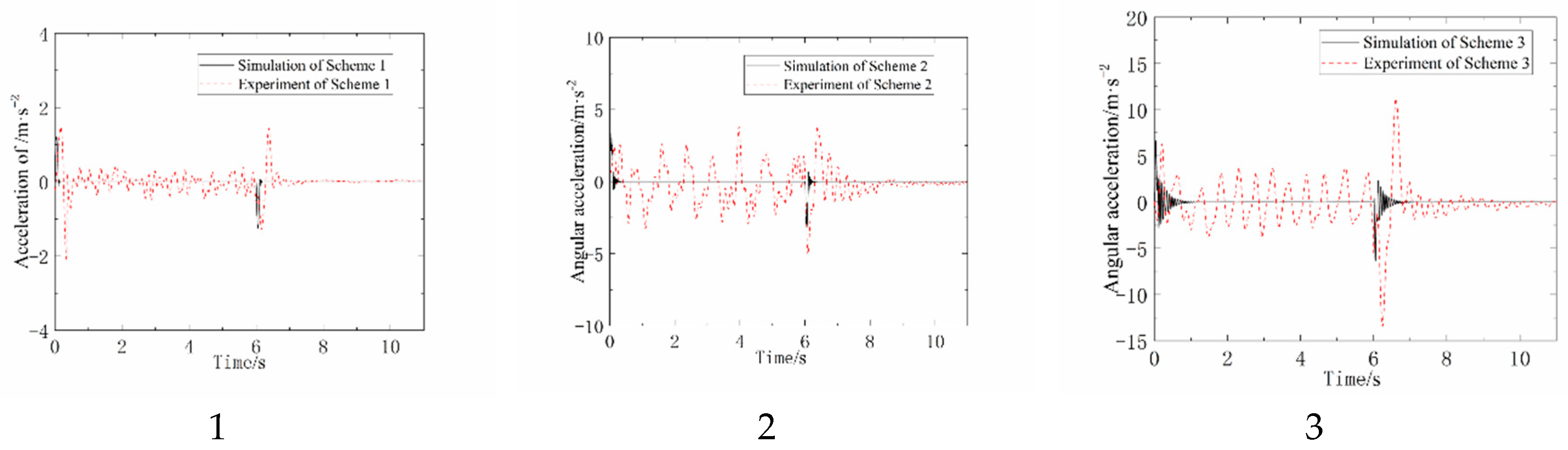
Figure 18. Acceleration before and after interface prototype replacement.

Disclaimer/Publisher’s Note: The statements, opinions and data contained in all publications are solely those of the individual author(s) and contributor(s) and not of MDPI and/or the editor(s). MDPI and/or the editor(s) disclaim responsibility for any injury to people or property resulting from any ideas, methods, instructions or products referred to in the content.

© 2024 by the authors. Licensee MDPI, Basel, Switzerland. This article is an open access article distributed under the terms and conditions of the Creative Commons Attribution (CC BY) license (http://creativecommons.org/licenses/by/4.0/).

Copyright: This open access article is published under a Creative Commons CC BY 4.0 license, which permit the free download, distribution, and reuse, provided that the author and preprint are cited in any reuse.

MDPI Initiatives

Important Links

Choose an area of interest and we will send you notifications of new preprints at your preferred frequency.

Disclaimer

Research on Deployment Process Dynamics and Vibration for Replaceable Interface Mast

Abstract

1. Introduction

2. Materials and Methods

2.1. Description of the movement of the shell unit

2.2. Deformation modeling of shell units

2.3. Flexible interface dynamics model

2.4. Dynamics model of the mast deployment process with replaceable interface

2.5. Fixed Constraints

2.6. Rotation constraints

2.7. Mast system dynamics equation

3. Analysis of the effect of nonlinear parameters on mast deployment

3.1. Non-linear effects of structural configuration

3.2. Non-linear effect of different shell thickness

3.3. Driving law non-linear influence

3.4. Experimental analysis of replaceable mast deployment

4. Conclusion

Author Contributions

Funding

Conflicts of Interest

References

MDPI Initiatives

Important Links

Subscribe