9.4 Inside a black hole
9.5 Black holes are true generators of matter in the universe
We will propose a generalization of the ADS/CFT correspondence. Here we hypothesize that we replace the ADS/CFT correspondence with a general equation given by DST = EFQT duality.
ADS is replaced by DST; DST represents a theory of quantum gravity associated with the theory of the generalization of the Boltzmann´s constant in curved space-time.
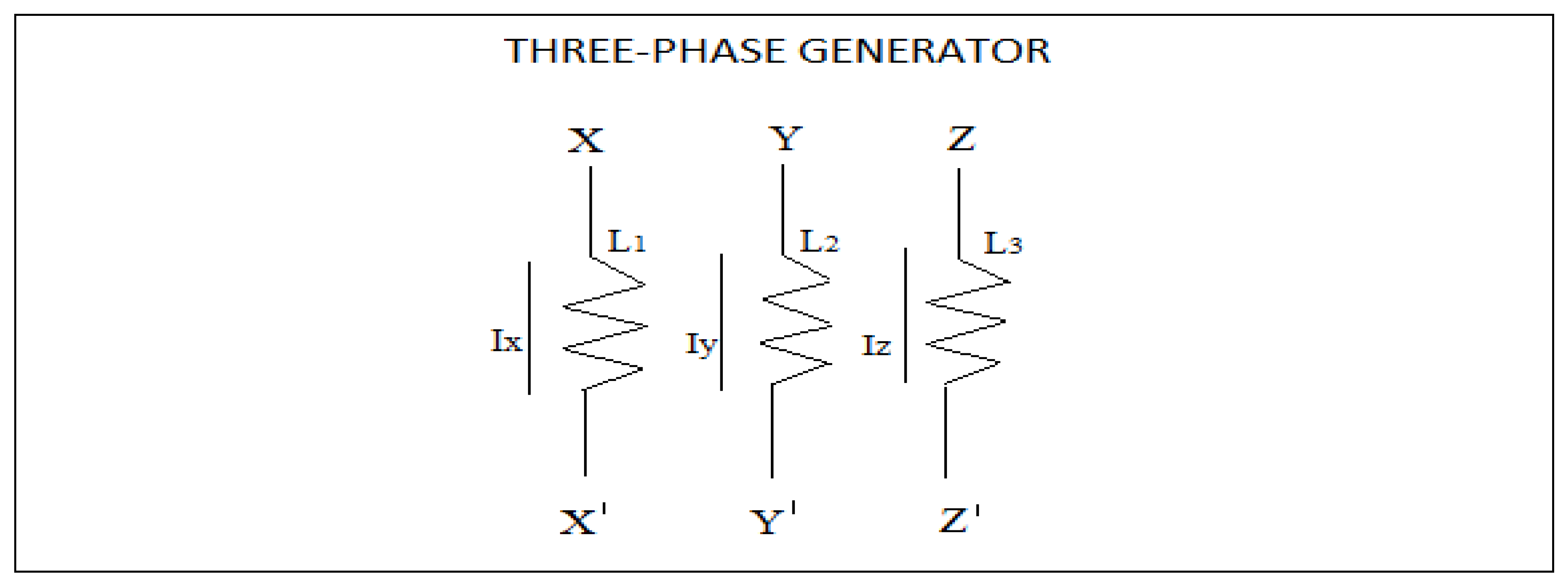
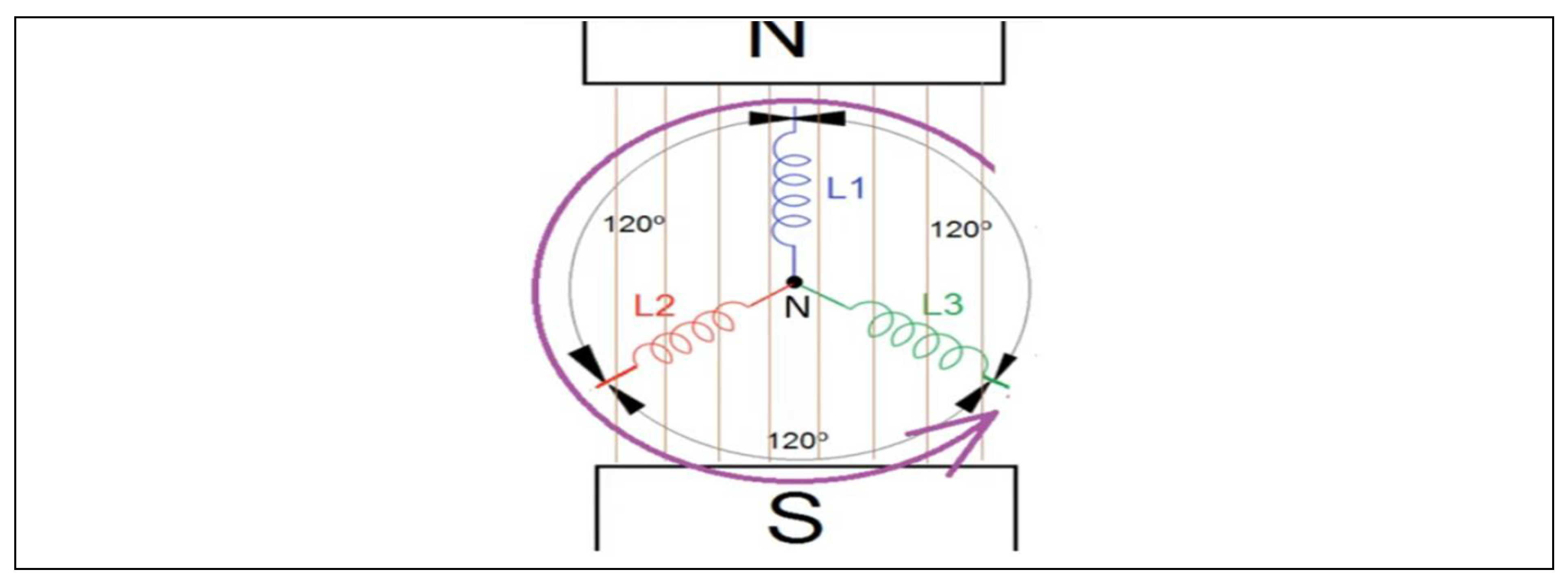
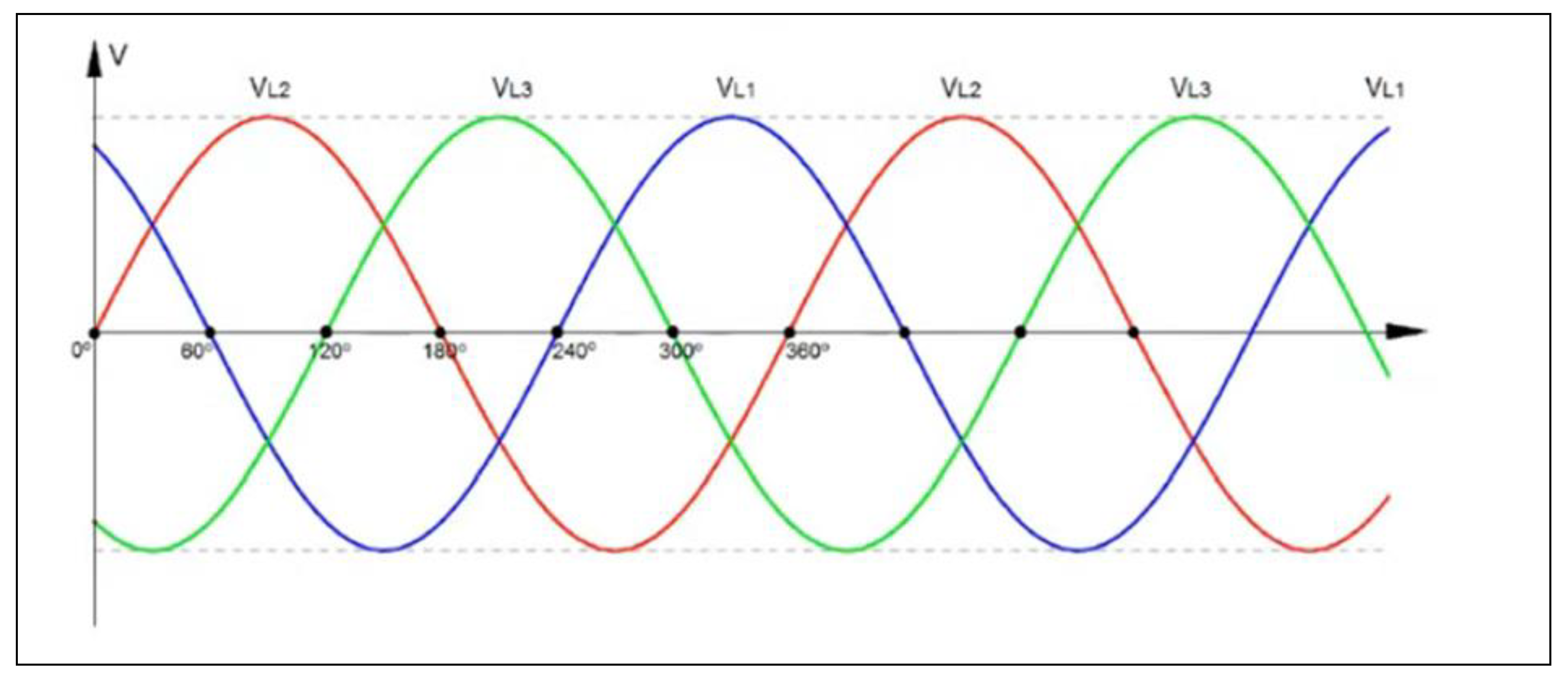
CFT is replaced by EFQT. EFQT represents unique electromagnetic field quantum theory, which unites the electromagnetic field theory, the weak field theory and the strong field theory and is associated with the theory: Electrical-Quantum Modelling of the Neutron and Proton as a Three-Phase Alternating Current Electric Generator.
Here we put forward the hypothesis that the equation DST = EFQT, represents the theory of everything, is the equation that unites gravity and quantum mechanics, this fact is achieved through the theory of the generalization of the Boltzmann´s constant in a curved space-time and the theory electrical-quantum modelling of the neutron and proton as a three-phase alternating current electric generator
We can represent it using the following general equations:
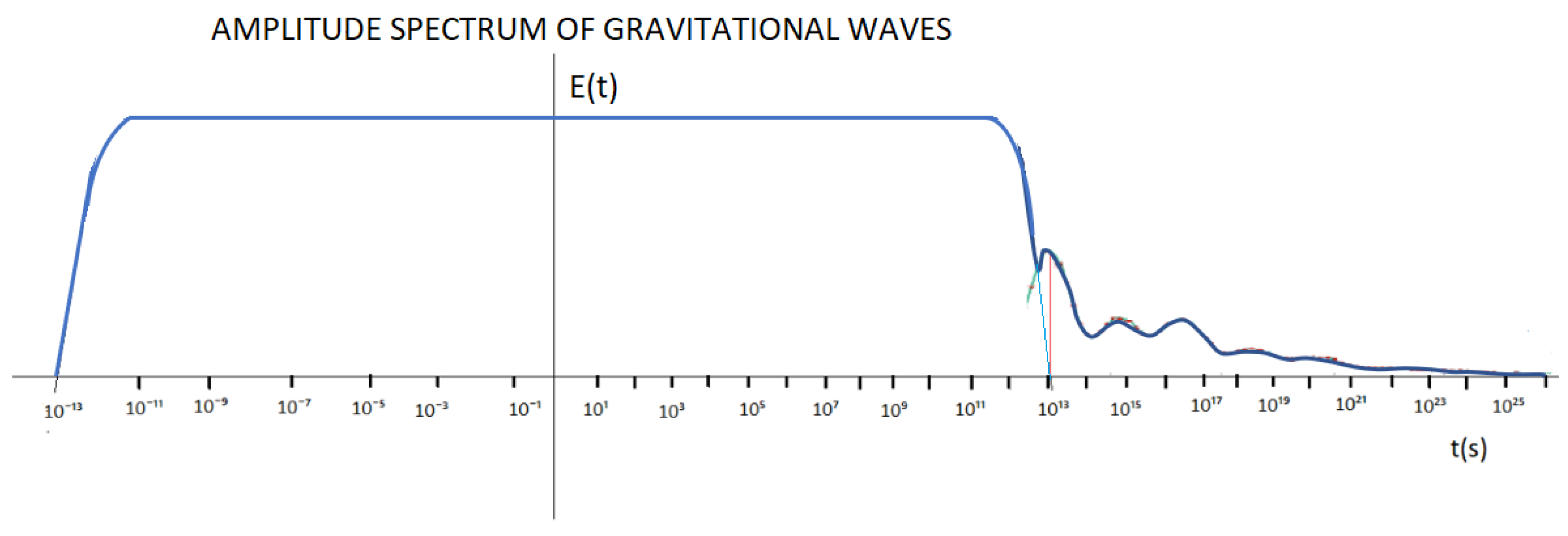
We will describe simple equations that represent the electromagnetic wave spectrum.
Eε = h x fε
Cε = λε x fε
Eε = h x Cε / λε
Eε = Kʙε x Tε
Kʙε = 1.38 10⁻²³ J/K
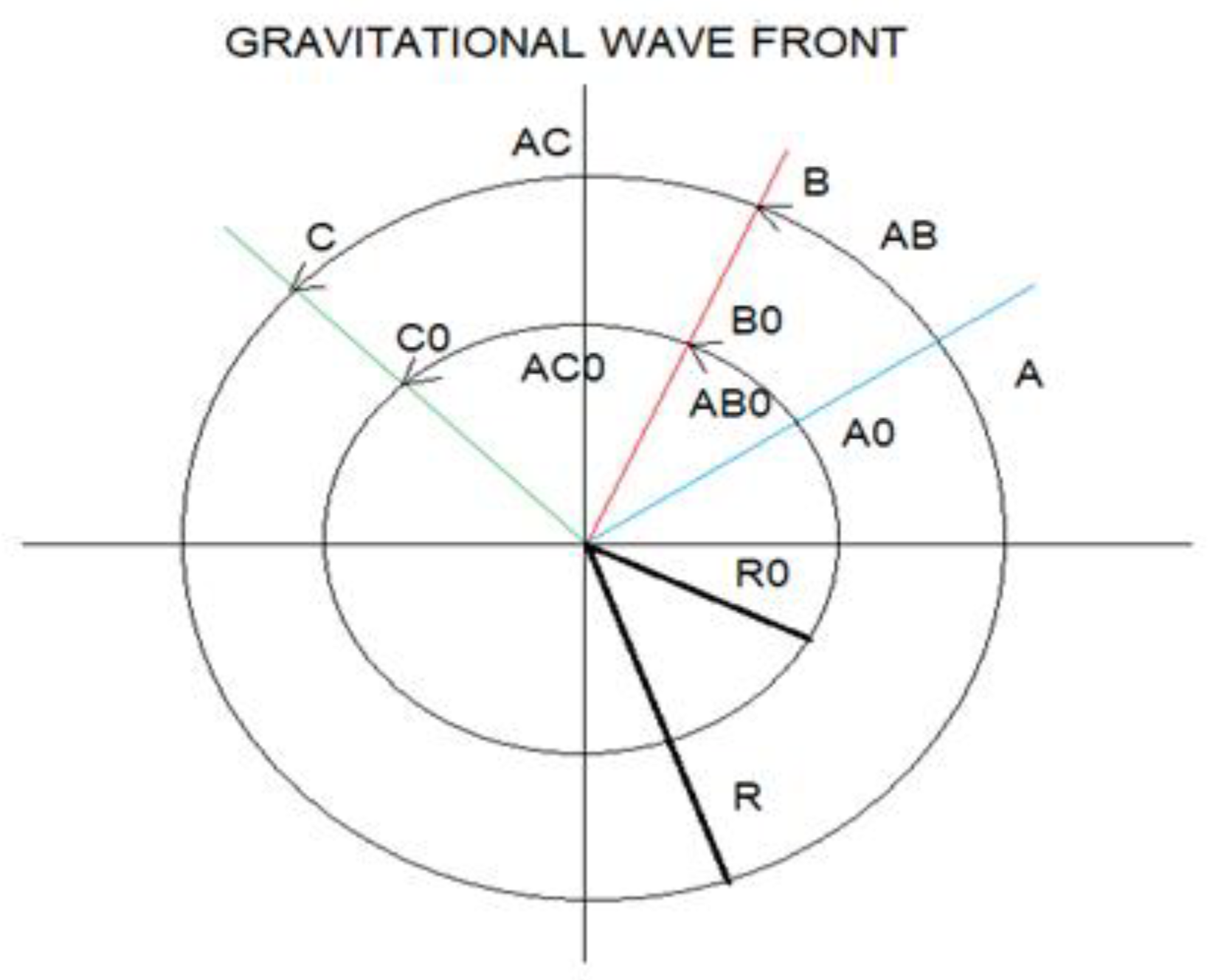
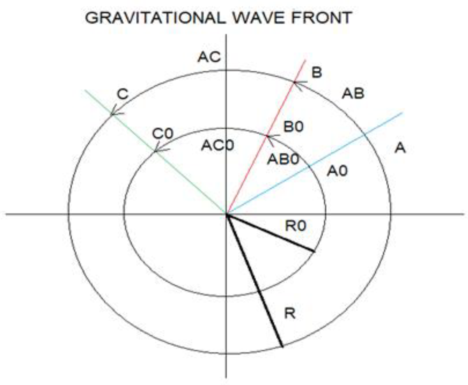
We will describe simple equations that represent the gravitational wave spectrum.
Eɢ = h x fɢ
Cɢ = λɢ x fɢ
Eɢ = h x Cɢ / λɢ
Eɢ = Kʙɢ x Tɢ
Kʙɢ = 1.38 10⁻²³ J/K > Kв ef > 1.78 10⁻⁴³ J/K
In the paper: RLC Electrical Modelling of Black Hole and Early Universe. Generalization of Boltzmann’s Constant in Curved Space-Time, we explain the origin of the universe, the origin of cosmic inflation, the origin of dark matter and the origin of dark energy.
In the paper: Theory of the Generalization of the Boltzmann’s Constant in Curved Space-Time. Shannon-Boltzmann Gibbs Entropy Relation and the Effective Boltzmann’s Constant, we explain how we can quantify the curvature of space-time and show using the Shannon-Boltzmann-Gibbs entropy relation that information is conserved.
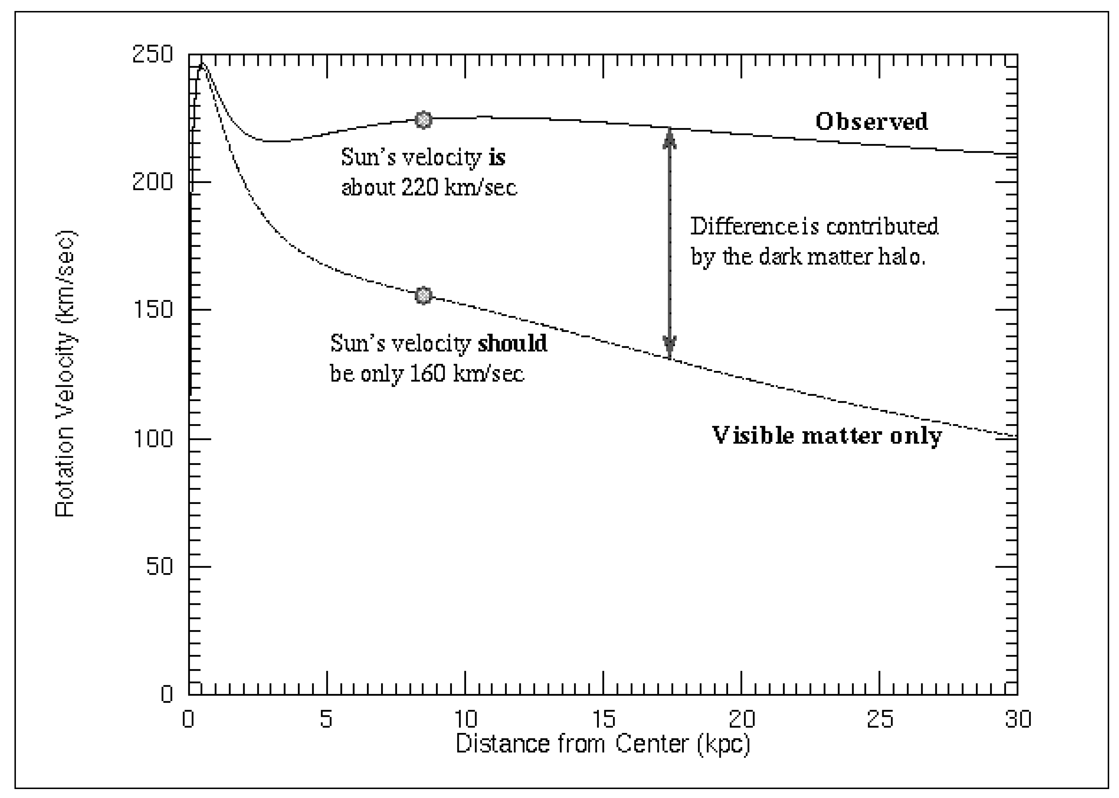
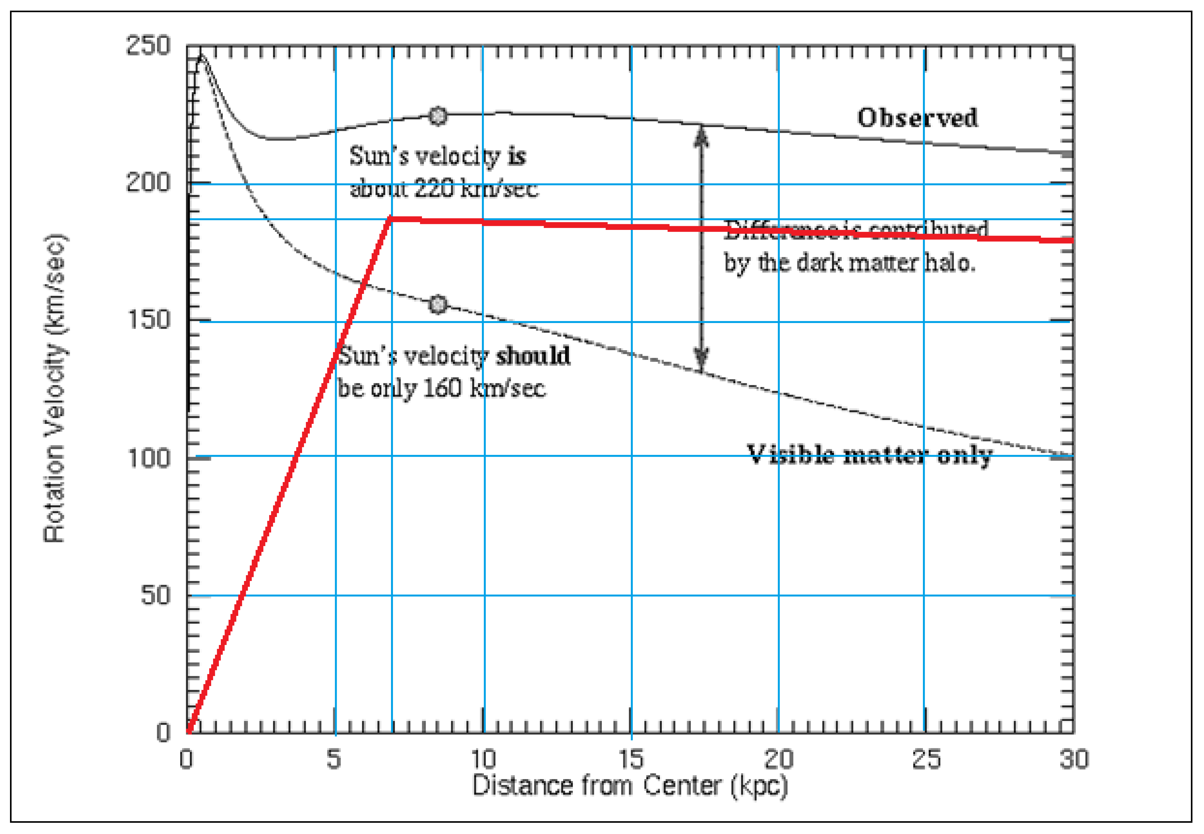
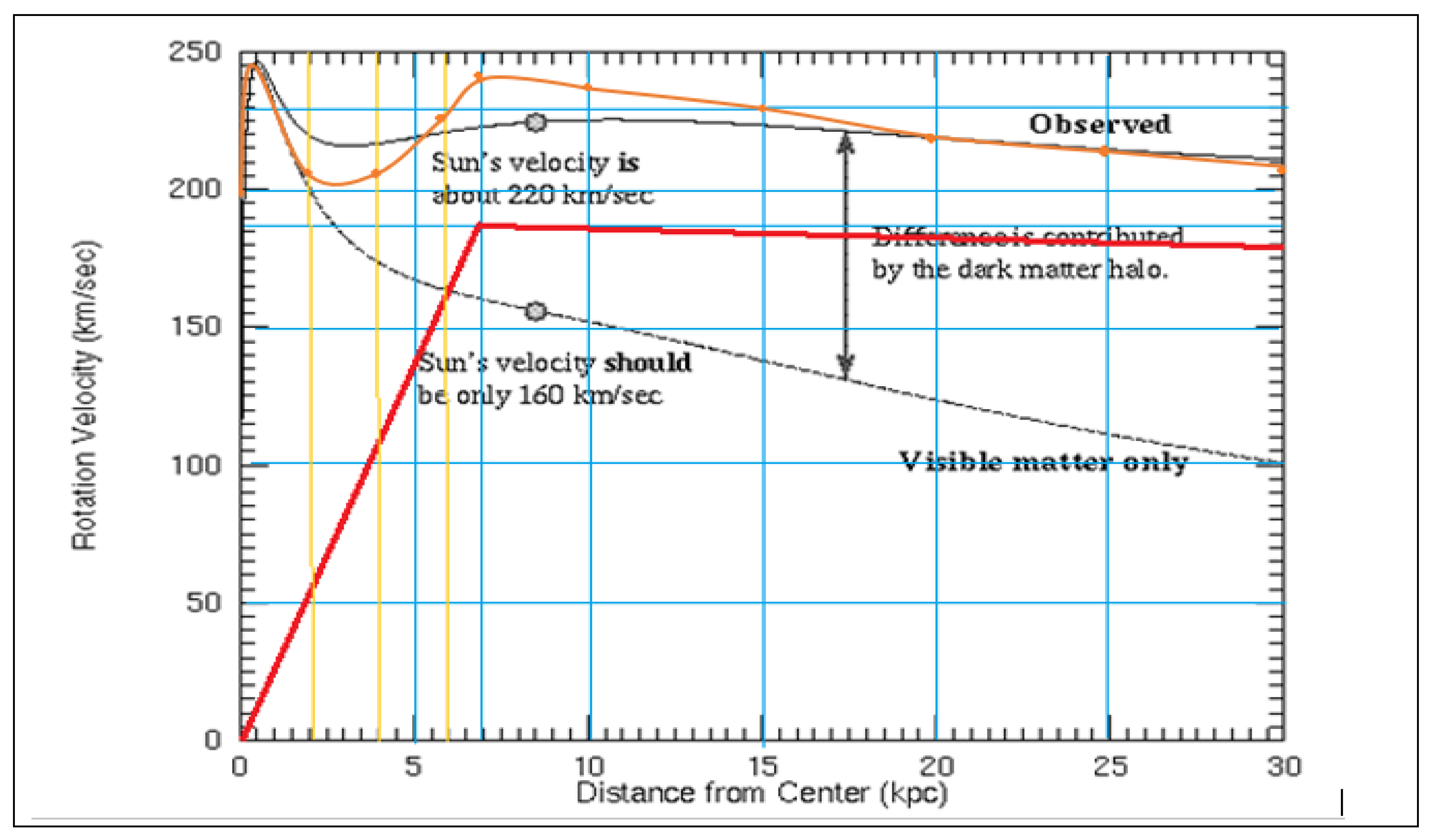
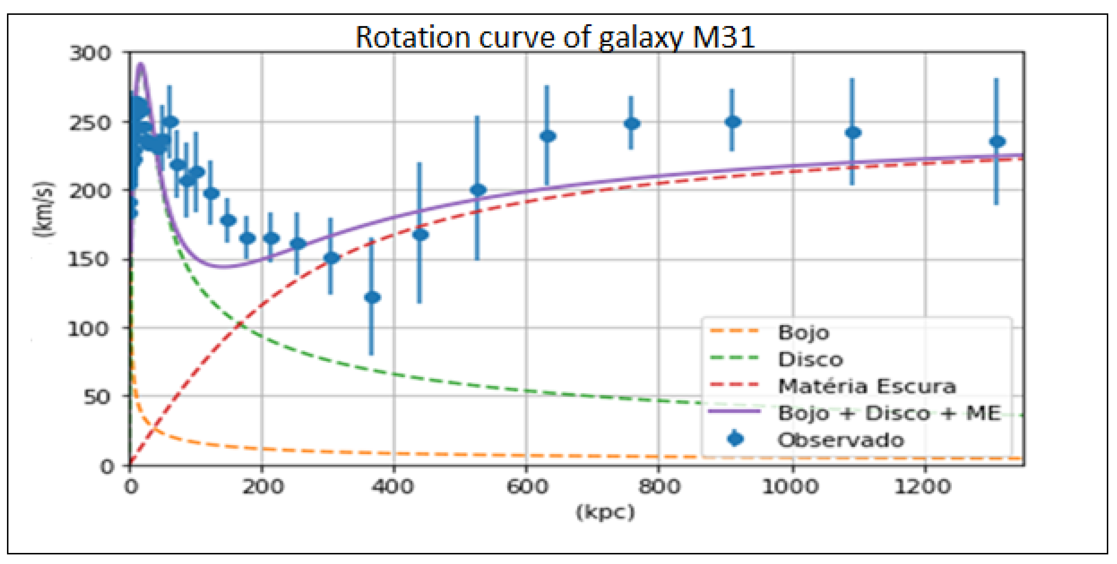
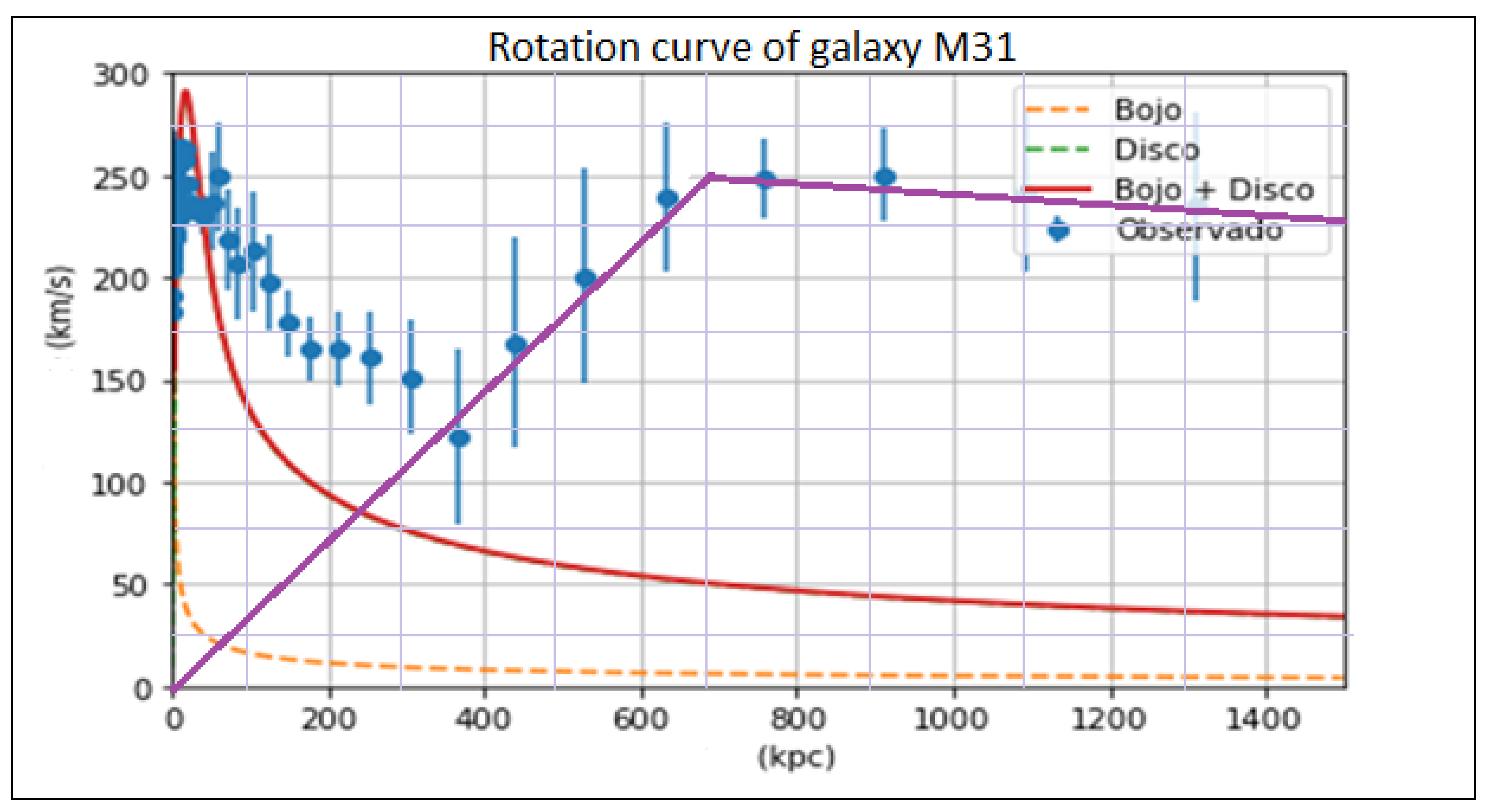
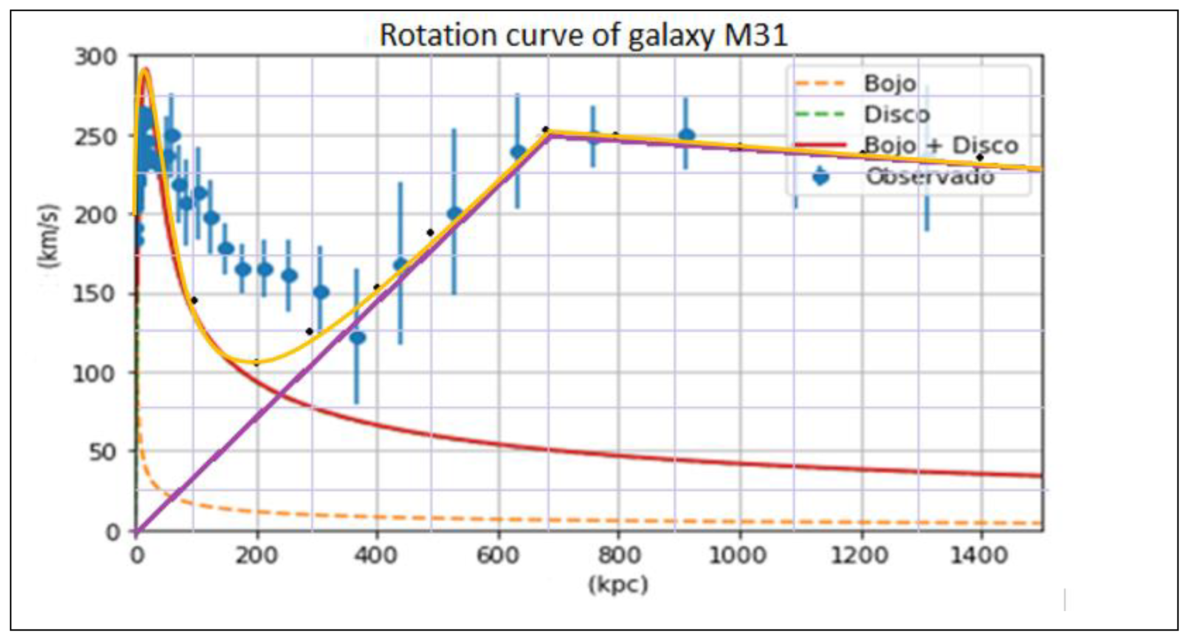
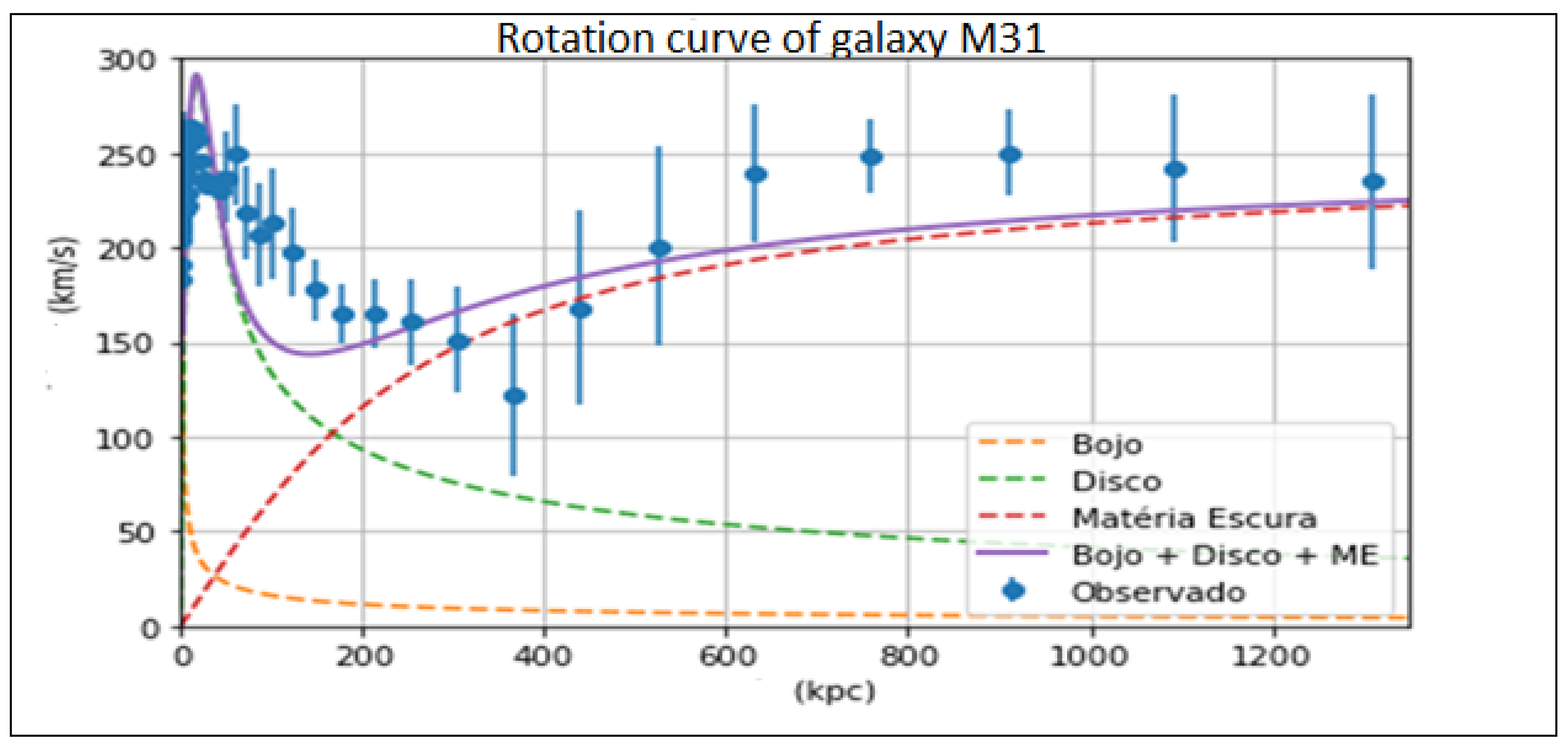
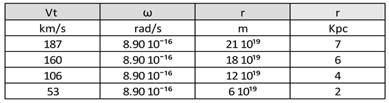
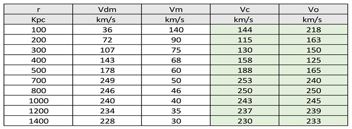
In the paper: RC Electrical Modelling of Black Hole. New Method to Calculate the Amount of Dark Matter and the Rotation Speed Curves in Galaxies, we explain how we can calculate the amount of dark matter in a galaxy and how we can model the rotation curves of a galaxy using a new method.
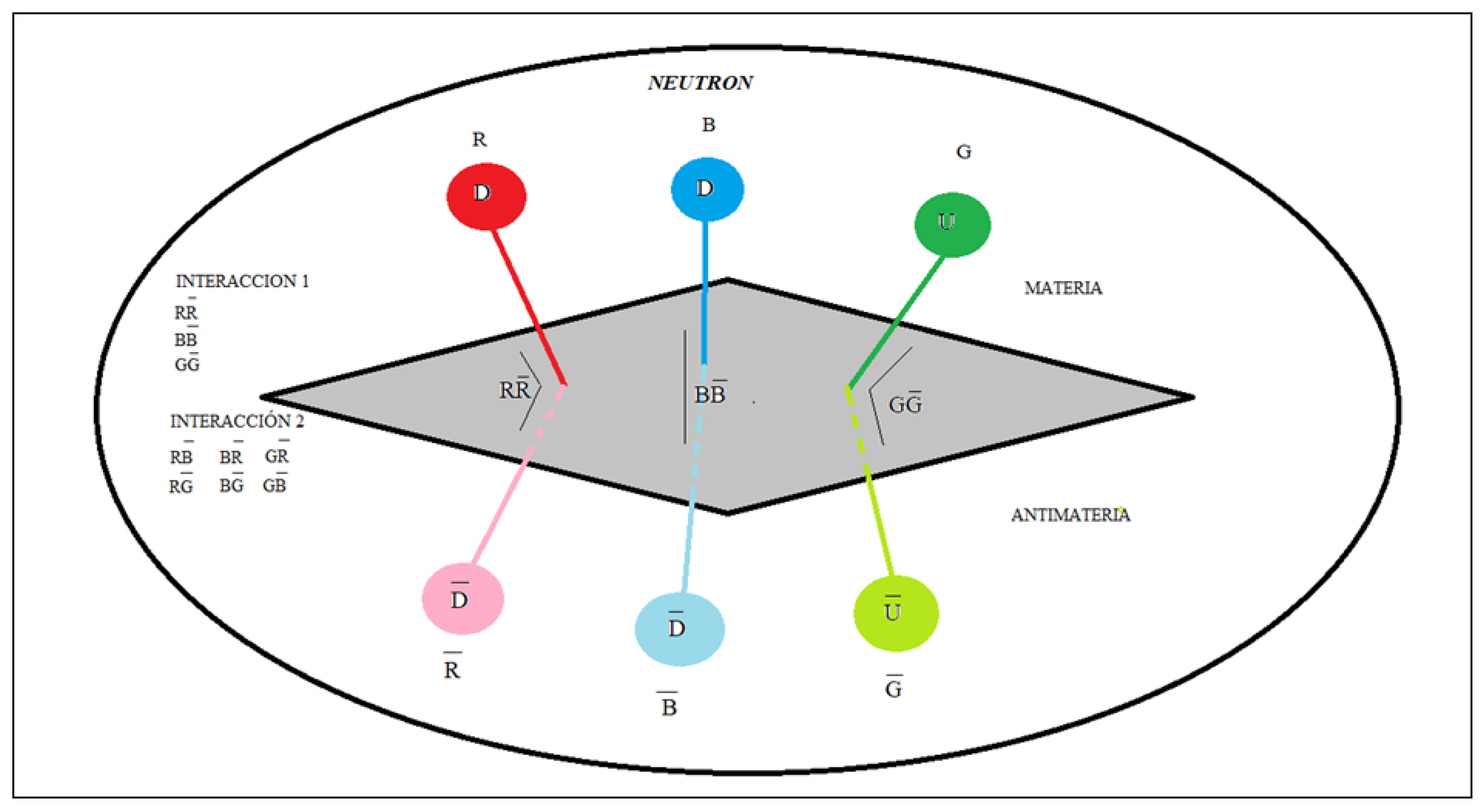
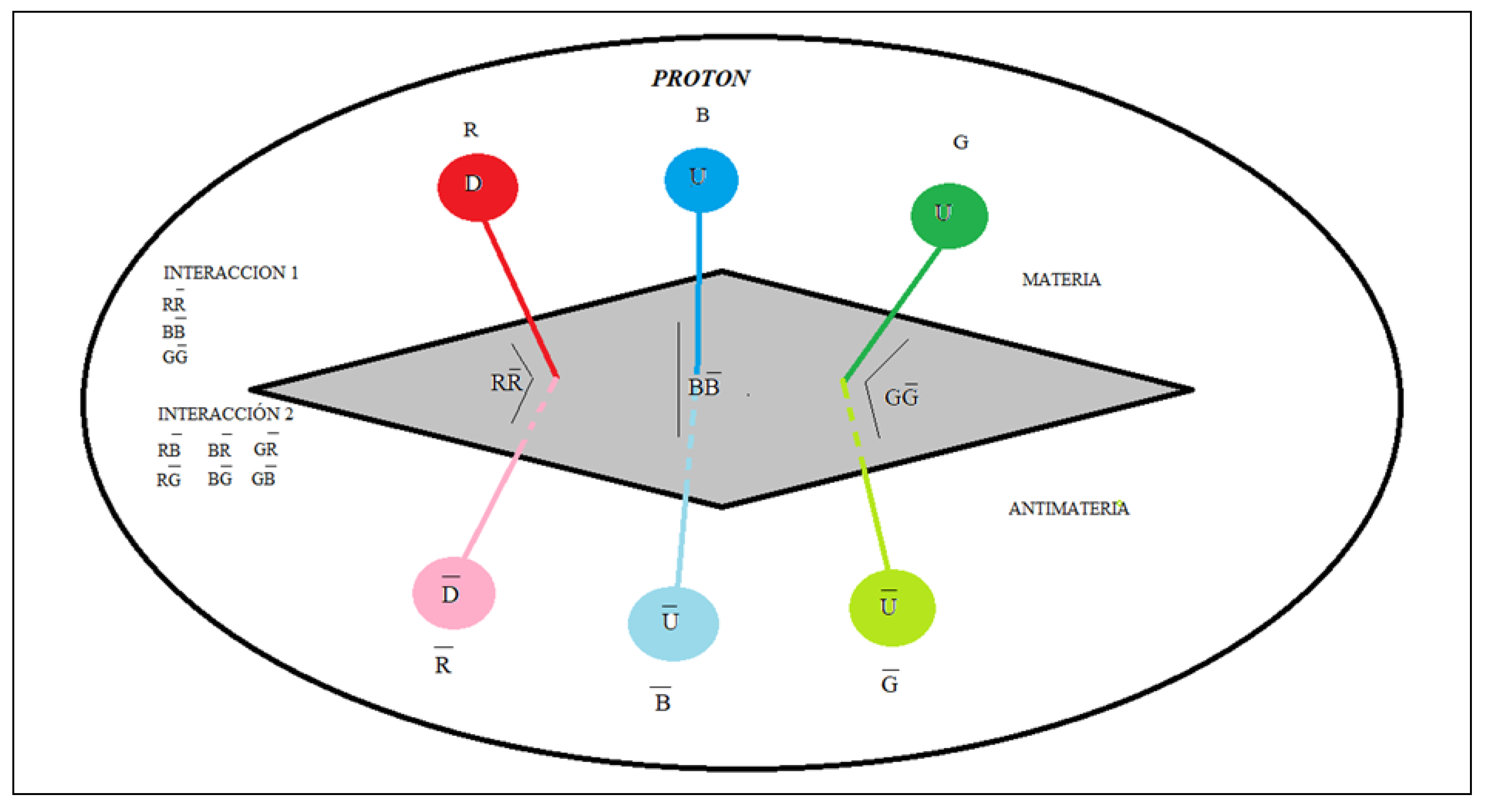
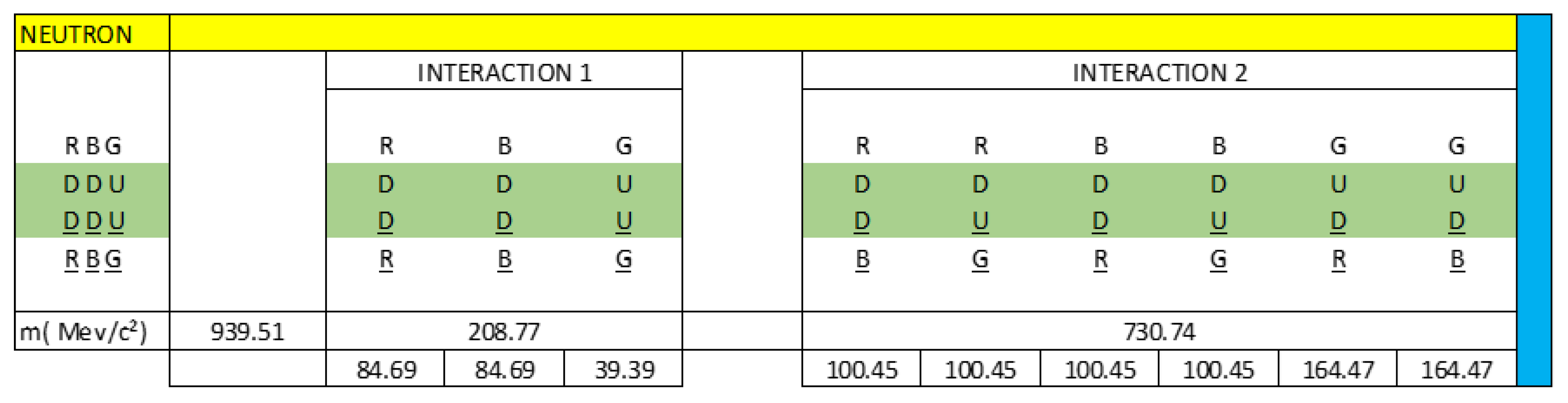
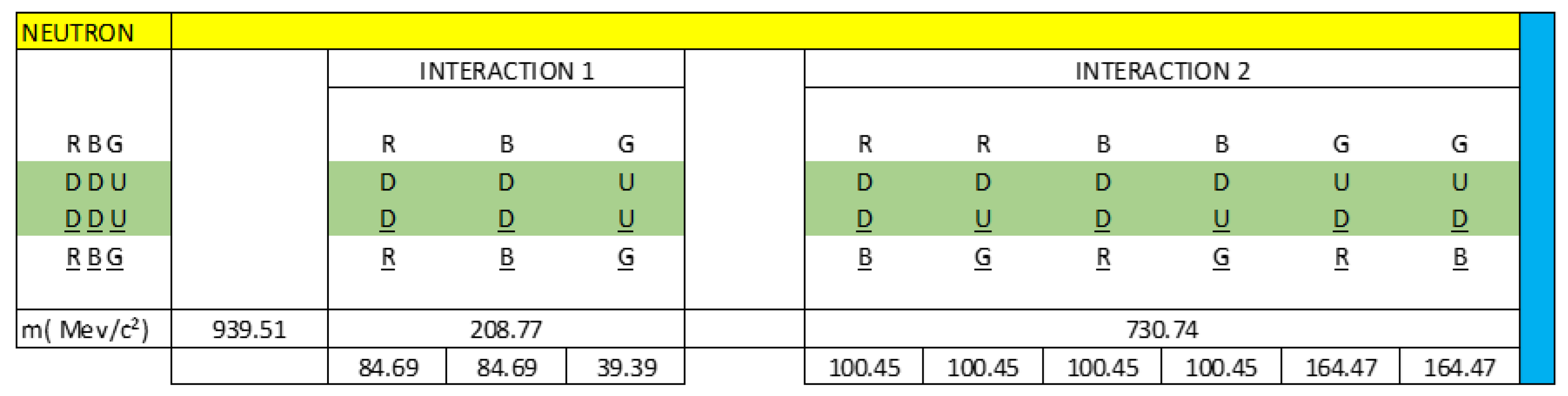
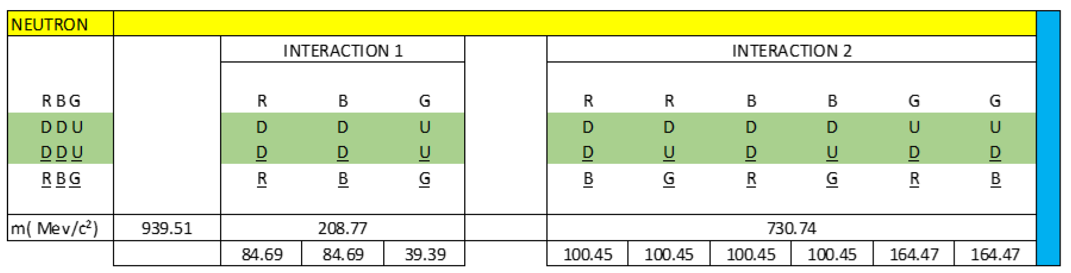
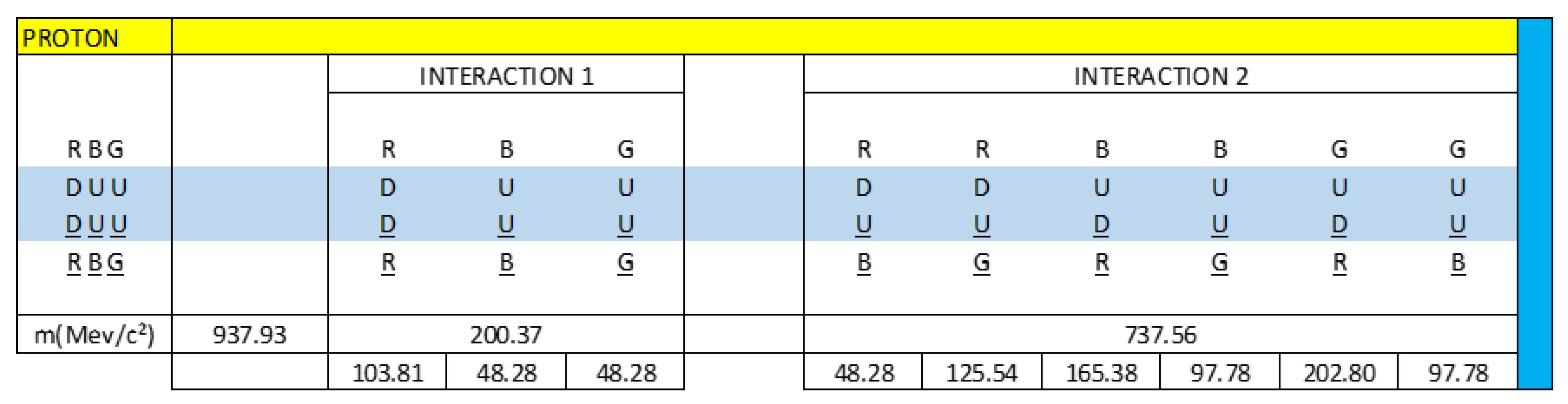
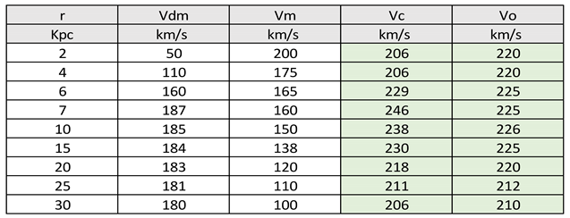
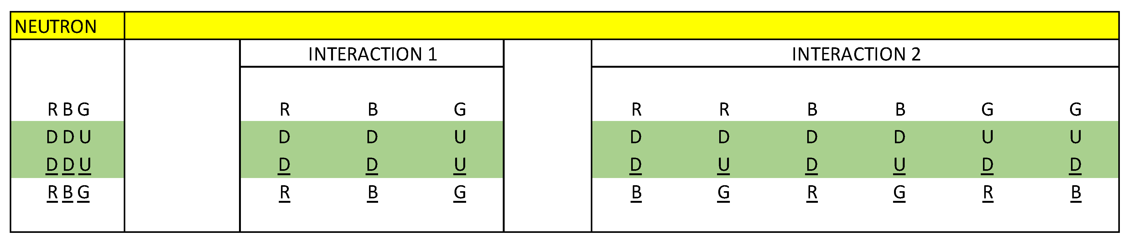
In the paper: Electrical-Quantum Modelling of the Neutron and Proton as a Three-Phase Alternating Current Electric Generator. Determination of the Number of Quarks-Antiquarks-Gluons and Gravitons, inside a Neutron; we explain how the mass is generated (we calculate the number of quarks-antiquarks-gluons) and the gravity (we calculate the number of gravitons) in a neutron.
In the paper: Theory of Unification of the Interactions of Fundamental Forces: SU(3) x SU(2) --> U(1); we explain that electromagnetic, weak, strong and gravitational interactions; they can be replaced by a single electromagnetic force interaction.
In this paper: Generalization of the Standard Model. Theory of Everything (T.O.E.) version 1; we proposed a method to determine the origin of elementary particles and how matter/energy is related to gravity, this allowed us to generalize the correspondence ADS/CFT, for a general theory or theory of everything.
The theory of the generalization of the Boltzmann´s constant and the quantum-electrical modelling of the neutron and the proton as a three-phase alternating current electric generator, are the fundamental basis or pillar that allows us to unite the theory of general relativity and quantum mechanics.
This theory allows us to quantify space-time, it allows us to quantify the curvature of space-time, it does not allow us to unite the field theory of electromagnetic interactions, weak interaction, strong interaction and gravitational interaction in a single quantum field theory of electromagnetic interactions EFQT.
Finally, it allows us to generalize the ADS/CFT correspondence. It allows us to propose a universal theory or theory of everything, represented by the equation:
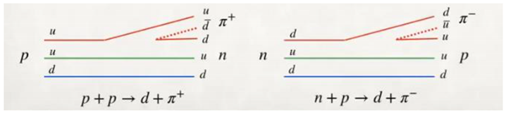
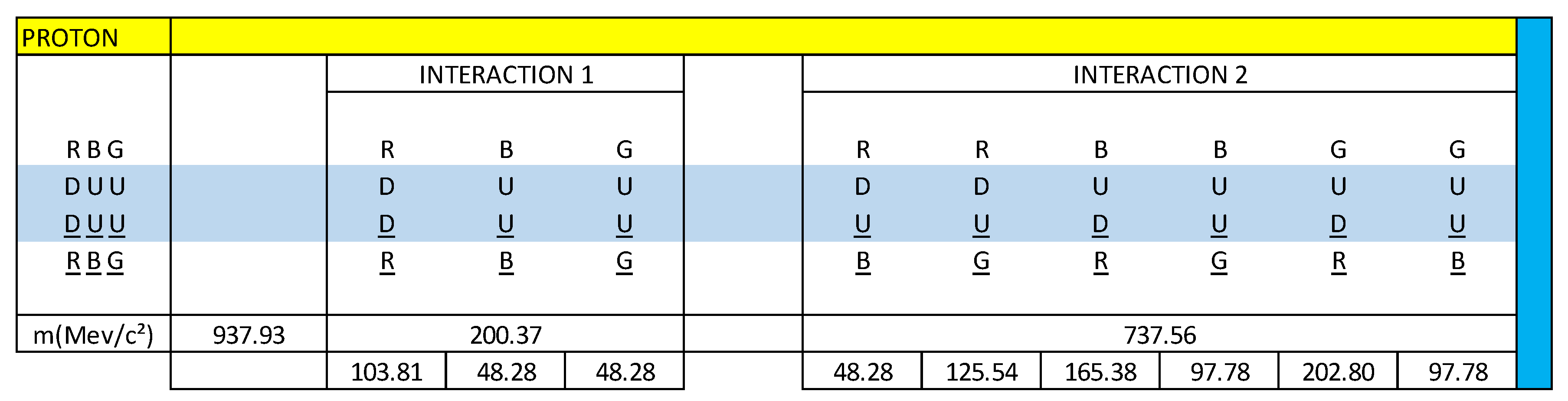
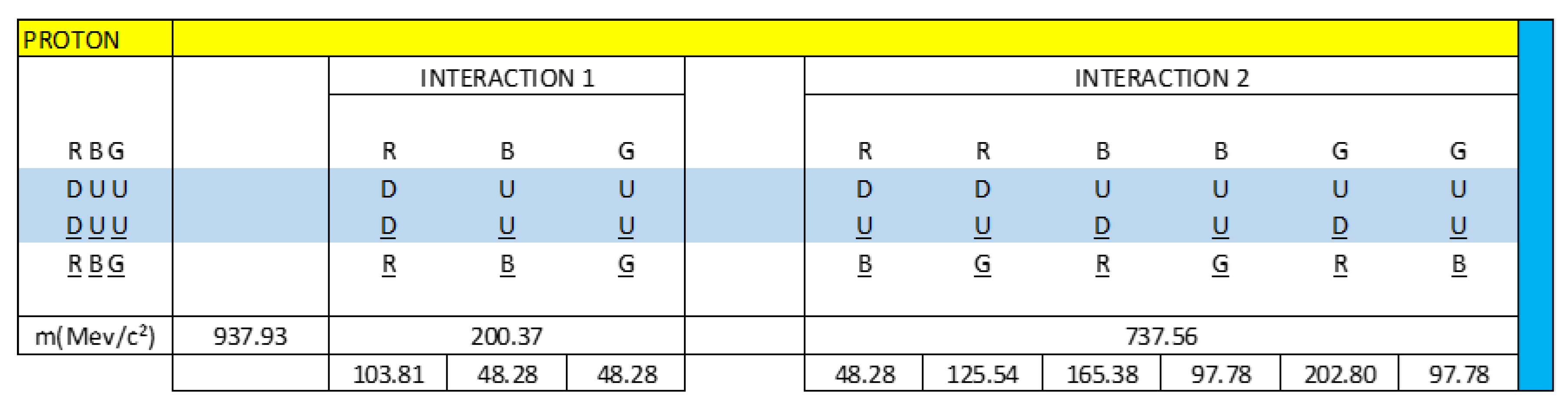
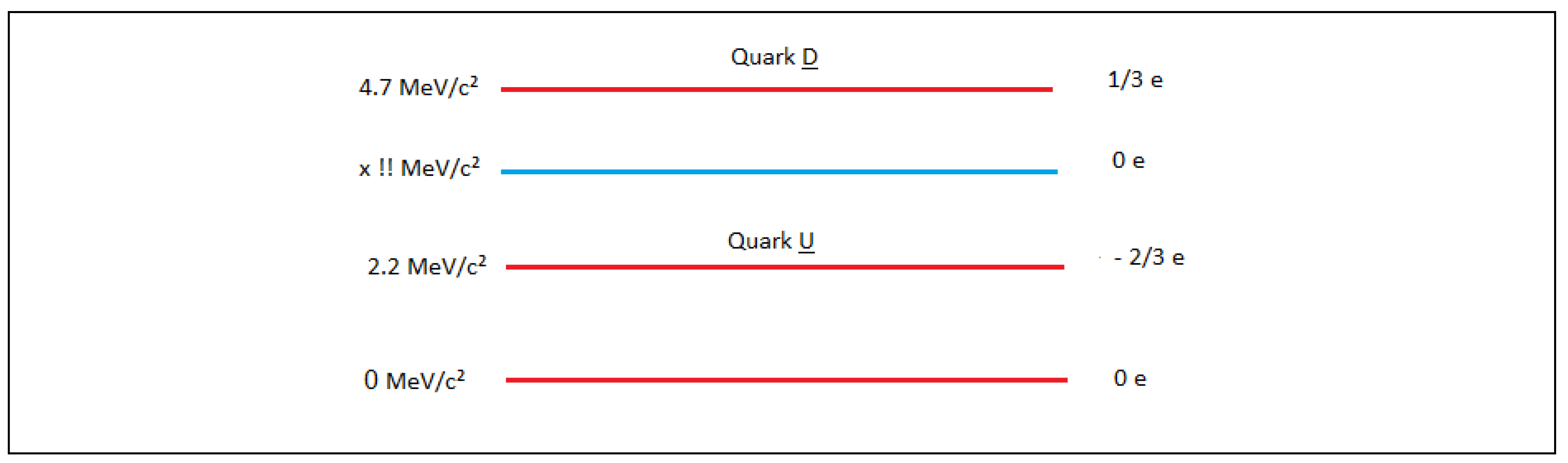
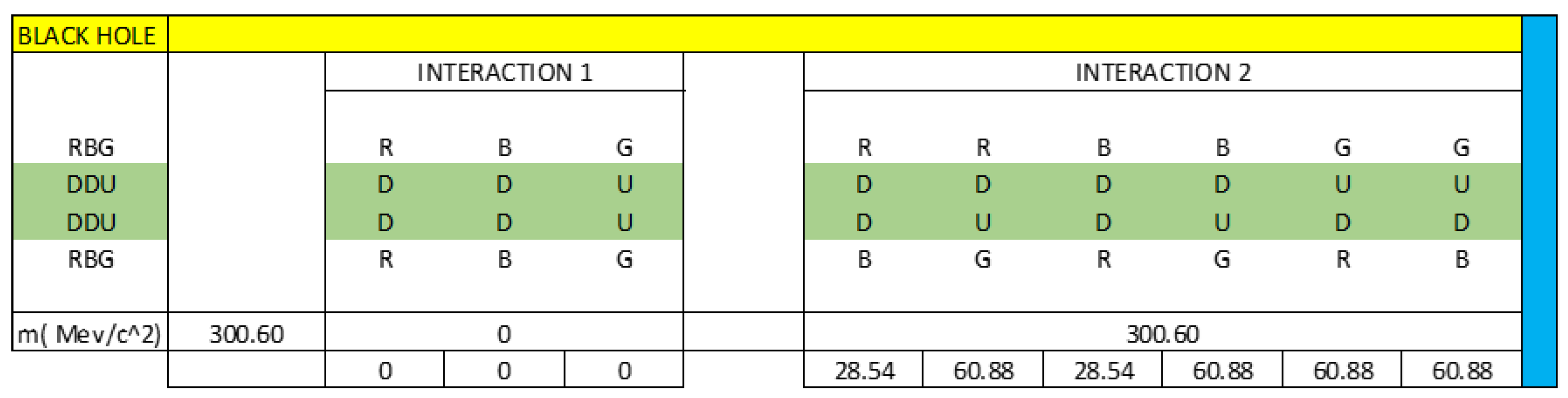
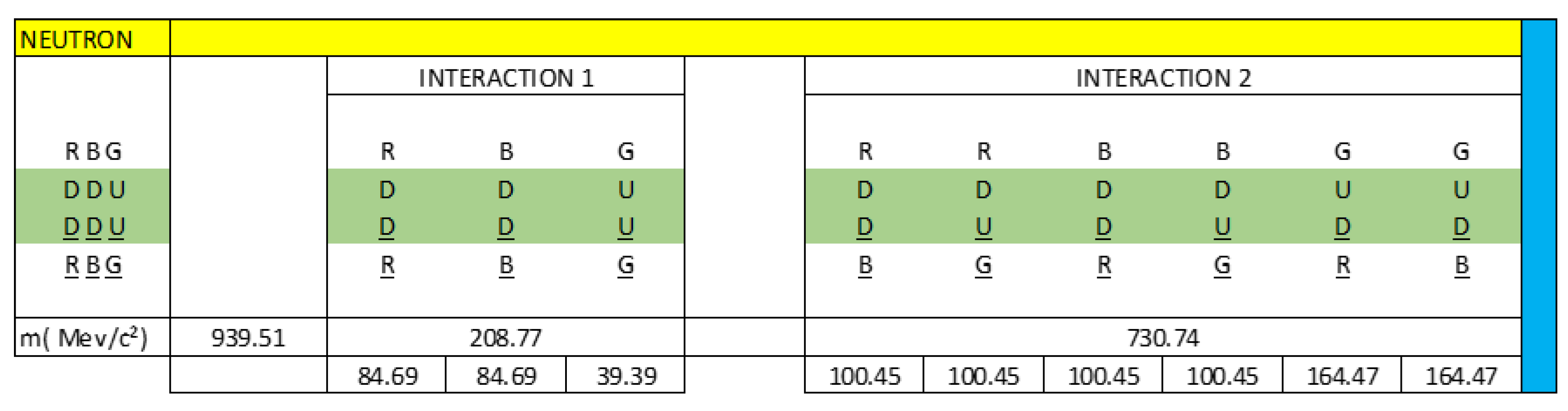
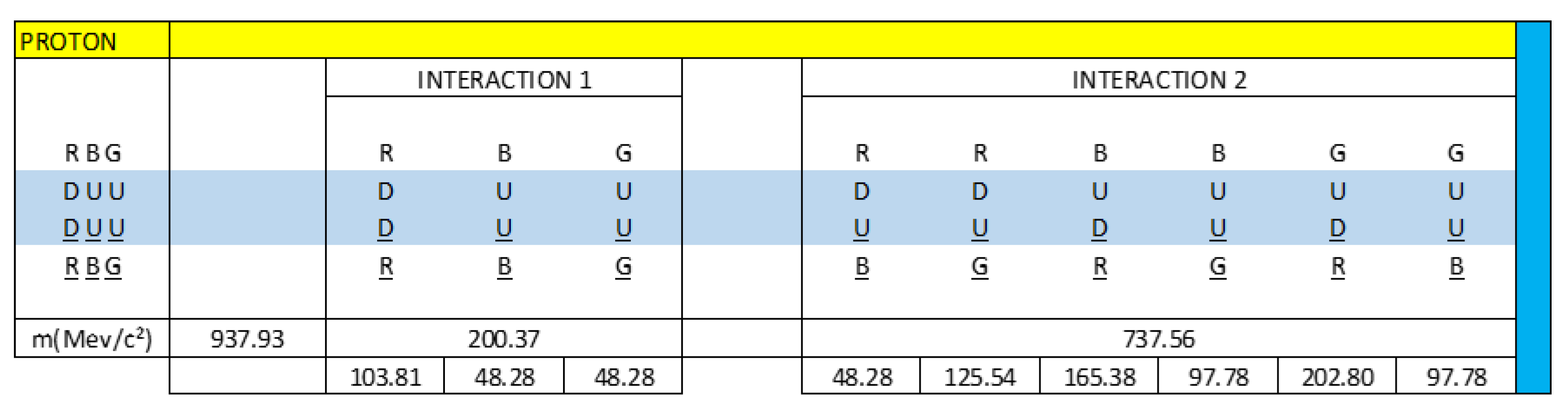
From the point of view of mass, the dynamics of both sides of the equation are dominated by quarks-antiquarks interactions (U, U, D, D).
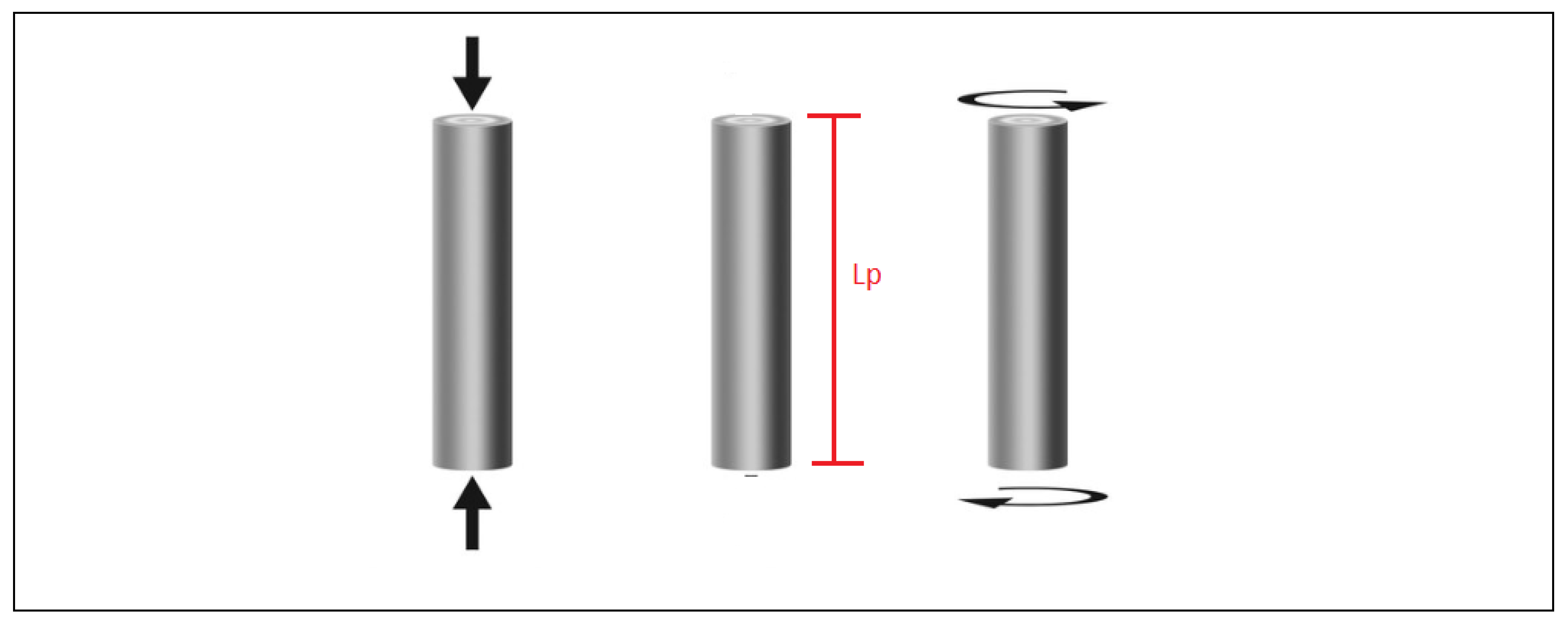
From the space-time point of view, the dynamics of both sides of the equation are dominated by the Planck constant. Outside a black hole, in the domain of the four existing force interactions, space-time is dominated by Planck length Lp; inside a black hole, in the domain of gravitational force, space-time is dominated by Lpԍ, where Lpԍ < Lp.
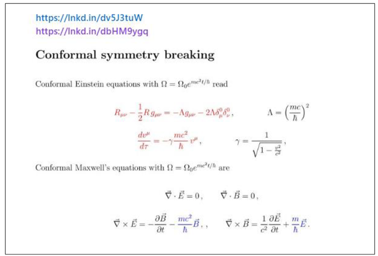
Higgs mechanism versus conformal mechanism
Gauge symmetry demands massless particles. The Higgs mechanism, on the other hand, is a technique for determining particle mass. In this case, the symmetry is broken at the price of providing particles with mass. This interaction occurs in a flat space. However, in curved space, particle mass may violate a symmetry known as conformal symmetry.
Breaking this symmetry is proven to give gravitons, photons, scalar fields (bosons), and Dirac particles mass in flat space. This mass is directly proportional to the conformal factor's (field) temporal derivative. The equation of motion of a particle in conformal space in curved space looks to be moving in a fluid (viscous), which may be the cause of inertia. There appears to be a background (conformal) field present with which particles and fields interact.
This text was posted by Arbab Ibrahim (Abdus Salam Intentional Centre for Theoretical Physics (ICTP)- Trieste-Italy), in QUANTUM PHYSICS.
This text, highlights the essence of this paper, shows us how the breakdown of symmetry in curved space-time provides mass to fermionic and bosonic particles as a function of temperature, as the temperature increases, the curvature of space-time increases; the fermionic and bosonic particles of the standard model acquire mass, it includes photons and gravitons to be clear.
It is precisely this reasoning that led us to generalize the ADS/CFT correspondence, where conformal quantum fields CFT, a particular case of quantum field theory, are generalized to the electromagnetic field quantum theory EFQT.
DST represents dynamic space-time, which we have shown is quantized; is on a plane of equality with EFQT, represented by electromagnetic field quantum theory; this duality, DST = EFQT, represents the equation of the theory of everything.
We are going to perform the following examples:
Example 1:
Quantification of space-time curvature
In the paper: RLC Electrical Modelling of Black Hole and Early Universe. Generalization of Boltzmann’s Constant in Curved Space-Time; we perform this example.
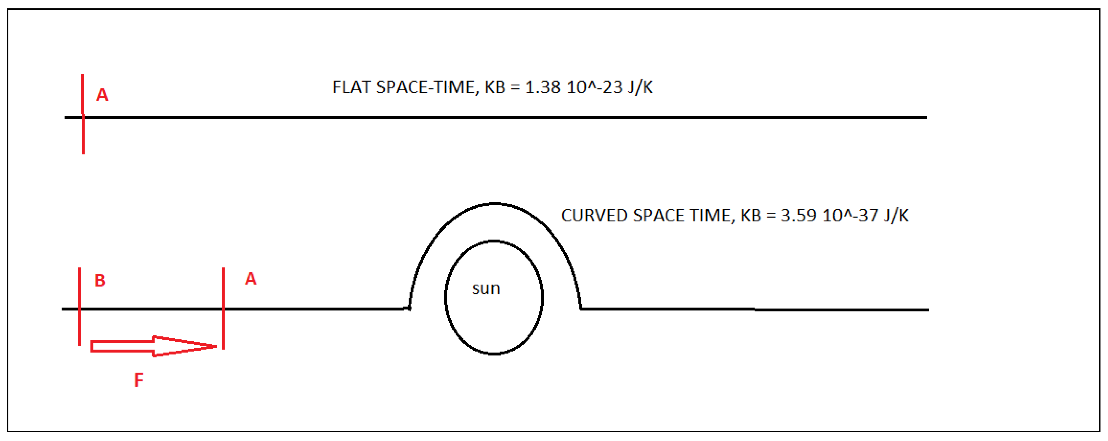
The observation of the 1919 solar eclipse in Brazil and Africa provided the first experimental proof of the validity of Albert Einstein's theory of general relativity. We will calculate the Boltzmann´s constant for the sun and show how it adjusts to the deviation found.
No solar eclipse has had as much impact in the history of science as that of May 29, 1919, photographed and analysed at the same time by two teams of British astronomers. One of them was sent to the city of Sobral, Brazil, in the interior of Ceara state; the other group go to the island of Principe, then a Portuguese territory off the coast of West Africa. The goal was to see if the path of starlight would deviate when passing through a region with a strong gravitational field, in this case the surroundings of the Sun, and by how much this change would be if the phenomenon was measured.
Einstein introduced the idea that gravity was not a gravitational force exchanged between matter, as Newton said, but a kind of secondary effect of a property of energy: that of deforming space-time and everything that propagates over it, including waves like light. “For Newton, space was flat. For Einstein, with general relativity, it curves near bodies with great energy or mass”, comments physicist George Matsas, from the Institute of Theoretical Physics of the São Paulo State University (IFT- Unesp). With curved space-time, Einstein's calculated value of light deflection nearly doubled, reaching 1.75 arc-seconds.
The greatest weight should be given to those obtained with the 4-inch lens in Sobral. The result was a deflection of 1.61 arc-seconds, with a margin of error of 0.30 arc seconds, slightly less than Einstein's prediction.
Demonstration:
Let us calculate the Boltzmann´s constant for the Sun, Kʙs, curved space-time.
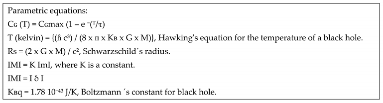
Hawking's temperature equation:
Kʙs = (h x c³) / (8 x π x Ts x G x Ms)
Where Kʙs is the Boltzmann´s constant for the sun, Ts is the temperature of the sun's core, G is the universal constant of gravity, and Ms is the mass of the sun.
Kʙs = (6.62 10⁻³⁴ x 27 10²⁴) / (8 x 3.14 x 1.5 10⁷ x 6.67 10⁻¹¹ x 1.98 10³⁰)
Kʙs = 3.59 10⁻³⁷ J/K, Boltzmann's constant of the sun.
We use the following equation:
Es = Kʙs x Ts
Es = 3.59 10⁻³⁷ x 1.5 10⁷
Es = 5.38 10⁻³⁰ J/K
We use the following equation:
Es = h x fs
fs = Es / h
fs = 5.38 10⁻³⁰ / 6.62 10⁻³⁴ = 0.81 10⁴ = 8.1 10³ Hz
fs = 8.1 10³ Hz
We use the following equation:
c = λs x fs
λs = c / fs
λs = 3 10⁸ / 8.1 10³
λs = 3.7 10⁴ m
We use the following equation:
Degree = λs / 360
Degree =102.77 m
We use the following equation:
Arc-second = degree / 3600
Arc-second = 102.77 m / 3600 = 0.0285 m
1.61 arc-second = 0.0458 m
1 inch = 0.0254 m
4 inch = 0.1016 m
With a 4-inch lens, we can measure the deflection produced by the 1.61 arc-second curvature of space-time, which was predicted by Albert Einstein's theory of general relativity, and corresponds to a wavelength λs = 3.7 10⁴ m, a frequency fs = 8.1 10³ Hz, for an effective Boltzmann´s constant of the sun Kʙs = 3.59 10⁻³⁷ J/K.
We will carry out the same calculations for Kʙ = 1.38 10⁻²³ J/K, flat space-time.
Kʙ = 1.38 10⁻²³ J/K
We use the following equation:
E = Kʙ x Ts
E = 1.38 10⁻²³ x 1.5 10⁷
E = 2.07 10⁻¹⁶ J/K
We use the following equation:
E = h x f
f = E / h = 2.07 10⁻¹⁶ / 6.62 10⁻³⁴
f = 3.12 10¹⁷ Hz
We use the following equation:
c = λ x f
λ = c / f
λ = 3 10⁸ / 0.312 10¹⁸
λ = 9.61 10⁻¹⁰ m
We use the following equation:
Degree = λ / 360
Degree = 0.02669 10⁻¹⁰ m
We use the following equation:
Arc-second = degree / 3600
Arc-second = 7.41 10⁻¹⁶ m
Using the Boltzmann´s constant Kʙ = 1.38 10⁻²³ J/K, we cannot correctly predict by mathematical calculations the deflection of light given by Albert Einstein's general theory of relativity, to be measured in the telescope at Sobral.
Through the example given, we can conclude that the Boltzmann´s constant Kʙs = 3.59 10⁻³⁷ J/K fits the calculations of the deflection of light in curved space-time.
Example 2:
Quark-gluon viscosity
We ask ourselves, why do we use the Boltzmann´s constant of a black hole to calculate the viscosity of a quark-gluon plasma?
We will give the answer with an example where the plasma viscosity of quarks-gluons is calculated. For the non-perturbative regime, for very large gs tending to infinity, we are comparing two theories in which the Boltzmann´s constants are approximately equal.
For the case of the 11-dimensional ADS theory, where we introduce a black hole, Boltzmann's constant is equal to Kʙ = 1.38 10⁻⁴³ J/K. For the 10-dimensional CFT theory, in which we want to calculate the plasma viscosity of quarks-gluons, the Boltzmann´s constant is of the order of 0.76 10⁻⁴¹ J/K > Kʙ > 1.78 10⁻⁴³ J/ K.
This tells us that we can use the ADS(DST) and CFT(EQFT) theories to calculate the plasma viscosity of quarks-gluons because both theories work in an almost identical non-perturbative regime, which is why whichever of the theories we use to calculate, the answer will be practically the same.
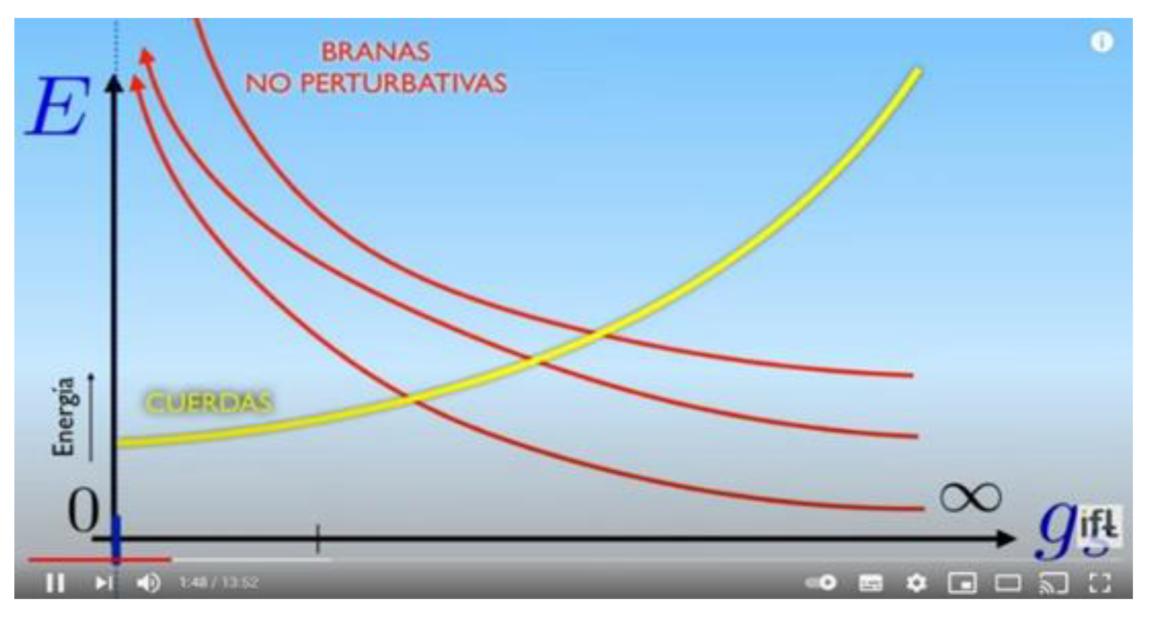
In strong coupling, in the limit where gs tends to infinity, that is, in the non-perturbative regime, we can reduce superstring theory to general relativity and with that we can simply use a theory of gravity in anti-de Sitter space ADS, to describe the strong coupling regime of a particle theory, we call dual QCD. This becomes a very useful duality.
In other words, whenever we use a CFT theory that works with a Boltzmann´s constant close to Kʙ = 1.78 10⁻⁴³ J/K, we can say that the duality ADS/CFT is fulfilled.
Using the following formula, we have:
VQGP = 3 h c² / (4 π Kʙ T)
ɲ/S = VQGP T
Where ɲ is shear viscosity, VQGP is Kinematic viscosity and ɲ/S is viscosity entropy ratio
Calculation of the viscosity of quark-gluon plasma:
Considering that a quark-gluon plasma has a Boltzmann´s constant given by:
Kʙ-eff = 1.78 10⁻⁴³ J/K
VQGP = 3 h c² / (4 π Kʙ-eff T), ħ = h / (2π)
c = 3 10⁸ m/s
T = 10¹³ K
h = 6,62 10⁻³⁴ (m² x kg)/s
VQGP = (3 x 6.62 10⁻³⁴ x 9 10¹⁶) / (4 x 3.14 x 1.78 10⁻⁴³ x 10¹³ x (2 x 3.14))
VQGP = (178.74 10⁻¹⁸) / (140.40 10⁻³⁰)
VQGP = 1.27 10¹²
ɲ/s = VQGP T; Applying the following formula we have:
ɲ/s = 1.27 10¹² 10¹³ = 1.27 10²⁵
ɲ/s = 1.27 10²⁵; viscosity-entropy relationship.
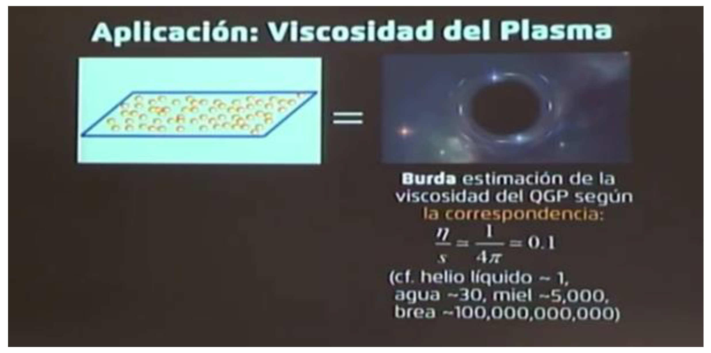
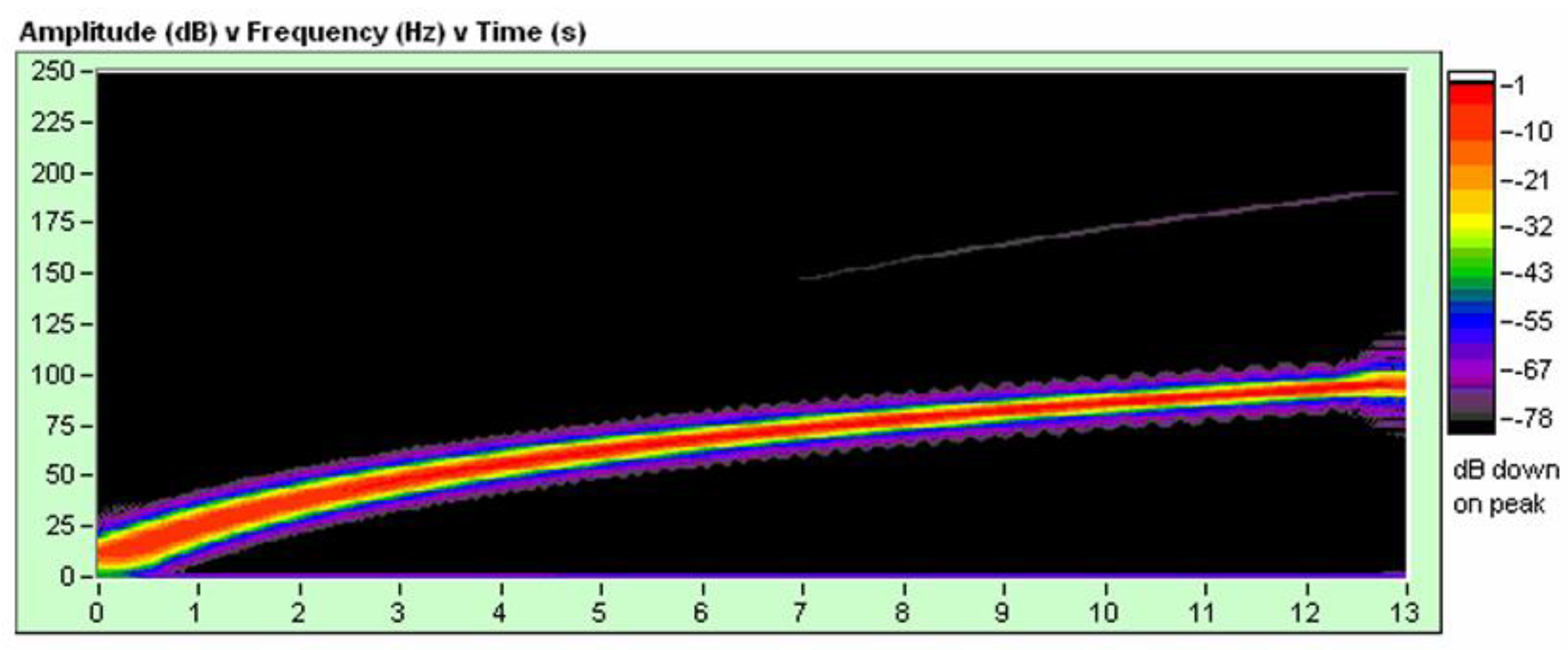
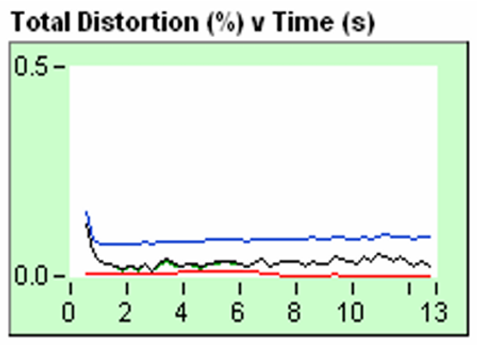
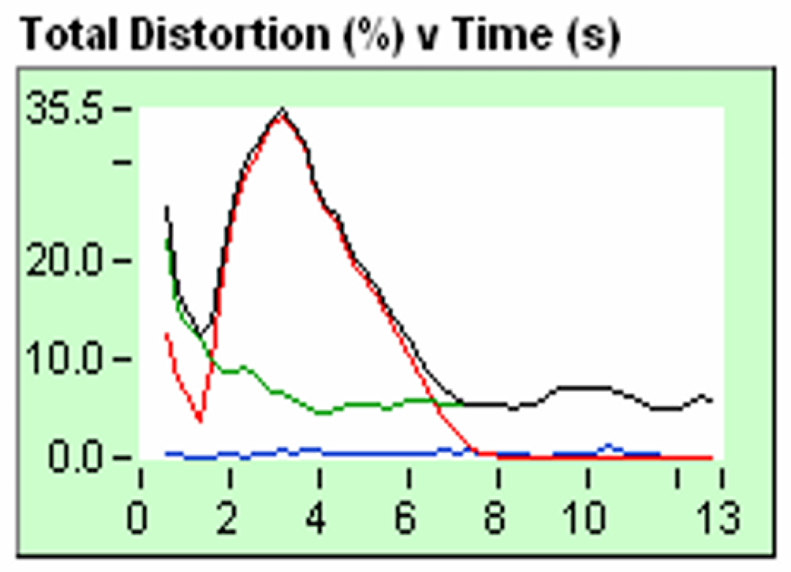
Figure 106.
QGP plasma viscosity applying the Maldacena correspondence.
Figure 106.
QGP plasma viscosity applying the Maldacena correspondence.
Considering that a quark-gluon plasma has a Boltzmann´s constant given by:
Kʙ = 1.78 10⁻²³ J/K
VQGP = 3 h c² / (4 π Kʙ-eff T), ħ = h / (2π)
c = 3 10⁸ m/s
T = 10⁻⁹ K
h = 6,62 10⁻³⁴ (m² x kg)/s
VQGP = (3 x 6.62 10⁻³⁴ x 9 10¹⁶) / (4 x 3.14 x 1.78 10⁻²³ x 10⁻⁹ x (2 x 3.14))
VQGP = (178.74 10⁻¹⁸) / (140.40 10⁻³²)
VQGP = 1.27 10¹⁴
ɲ/s = VQGP T; Applying the following formula we have:
ɲ/s = 1.27 10¹⁴ x 10⁻⁹ = 1.27 10⁵
ɲ/s = 1.27 10⁵; viscosity-entropy relationship.
If we look at
Figure 51, we will see that the viscosity of the QGP plasma by the holographic method is ɲ/s = 0.1, less than liquid helium (superfluid) and less than water. We ask ourselves, is this value correct? Could it be that a black hole with a density of approximately 10²¹ kg/m³, a density similar to that of QGP plasma, behaves like a superfluid whose viscosity is lower than that of liquid helium?
In the paper: RLC Electrical Modelling of Black Hole and Early Universe. Generalization of Boltzmann's Constant in Curved Space-Time; the critical temperature for the Bose-Einstein condensate of rubidium atoms was calculated for the following values of the Boltzmann´s constants, Kʙ = 1.38 10⁻²³ J/K and Kʙ = 1.78 10⁻⁴³ J/K; both values of the Boltzmann´s constant indicate that there are two types of temperatures that allow the creation of a Bose-Einstein condensate:
• Tc, min = 170 10⁻⁹ K, minimum critical temperature of the Bose-Einstein condensate for low temperatures, with rubidium atoms.
• Tc, max = 1.01 10¹³ K, maximum critical temperature of the Bose-Einstein condensate for high temperatures with rubidium atoms.
At this point, we have to clarify that a black hole is a QGP plasma, a high-temperature Bose-Einstein condensate in which the quarks behave as if they were free, generating a cascade of gluons of infinite energy, forming the state most energetic that exists in the universe.
If we look again atFigure 51, we see that the viscosityɲ/s = 10¹¹ for brea. In our calculation, for a black hole of 3 solar masses, a density of approximately 10²¹ kg/mᶾ, the value of the viscosity is of the order ofɲ/s = 10²⁵; I interpret that this value is more in line with reality, it is the correct value, taking into account the density.
Let's try to understand why the behaviour of the quark-gluon plasma resembles that of a superfluid. If we remember how we generate the scale factor of the Boltzmann´s constant, as matter gains energy and goes through the states of a white dwarf star, neutron star, until forming a QGP plasma; we see that the Boltzmann´s constant changes from 1.38 10⁻ ²³ J/K > Kʙ > 1.78 10⁻⁴³ J/K; this gives us an idea of how compacted or concentrated the mass is (gains energy) and how curved space-time is. This curvature of space-time is proportional to the amount of energy that the mass gains and we can compare it to a spring that compresses.
When we produce the QGP in a particle accelerator LHC, the quark-gluon plasma has stored energy but this state is not stable and at this point the QGP has an approximate Boltzmann´s constant Kʙ-eff = 1.78 10⁻⁴³ J/K. For curved space-time and matter to return to their stable state, the Boltzmann´s constant must go from Kʙ = 1.78 10⁻⁴³ J/K to 1.38 10⁻²³ J/K, that is, in this point all the energy stored in the compressed spring, is released until it reaches its natural state, that is, until the Boltzmann´s constant reaches the value of Kʙ = 1.38 10⁻²³ J/K. It is this energy that makes QGP look like a superfluid, but in reality, if we consider the scale factor of the Boltzmann´s constant, we will see that ɲ/s = 1.27 10²⁵ (viscosity-entropy relationship). The energies involved in this process are very great.
I can't imagine how something that has a density on the order of 10²¹ kg/mᶾ behaves like a superfluid with a lower viscosity than liquid helium.
Possibly, the Boltzmann´s constant Kʙ-eff is the response to the discrepancy that exists with the holographic method to calculate the viscosity of the QGP, ɲ/s = 0.1; I let the reader draw their own conclusions.
Example 3:
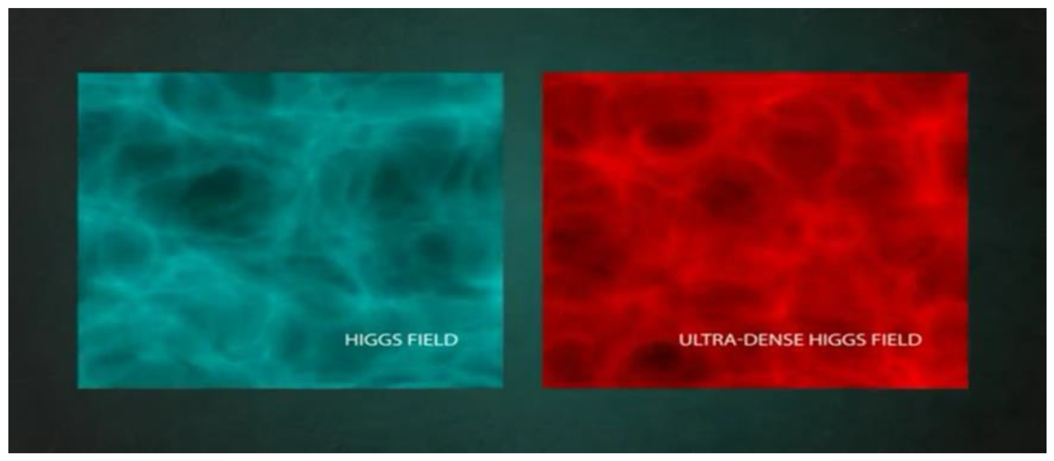
The two states of the Higgs field
By studying the Higgs field, theoretical physicists have discovered that the Higgs field, which permeates all of spacetime, exists in two states, in addition to the state known today; there is a second state thousands of times denser called the ultra-dense state of the Higgs field. This creates a potential problem, which is the possibility of a transition between the two states. We will analyse that this transition is almost impossible to happen.
First state of the Higgs field:
The Higgs field that we know today fills the entire space-time of our universe and together with the gravitational field, gives mass to the particles, for example, when the elemental energy corresponding to the electron moves in the Higgs field and the field gravitational, its interaction with the two fields gives the mass to the electron as we know it in the standard model table.
The Higgs boson is the excitation of the Higgs field; the Higgs field should not be confused with the Higgs boson.
The Higgs field has a value in vacuum and corresponds to:
H = 246 GeV (2.85 10¹⁵ K), this corresponds to a minimum potential energy V that gives stability to our current universe.
Second state of the Higgs field - Ultra dense state
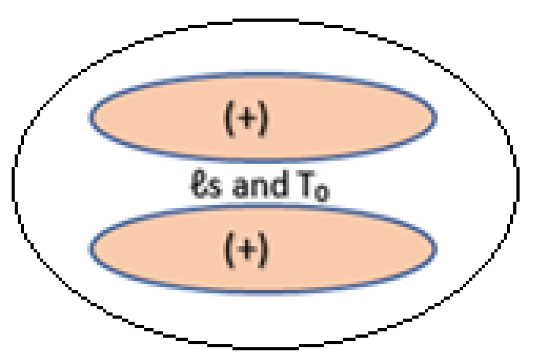
Hypothesis: I propose that the ultra-dense state of the Higgs field occurs inside black holes.
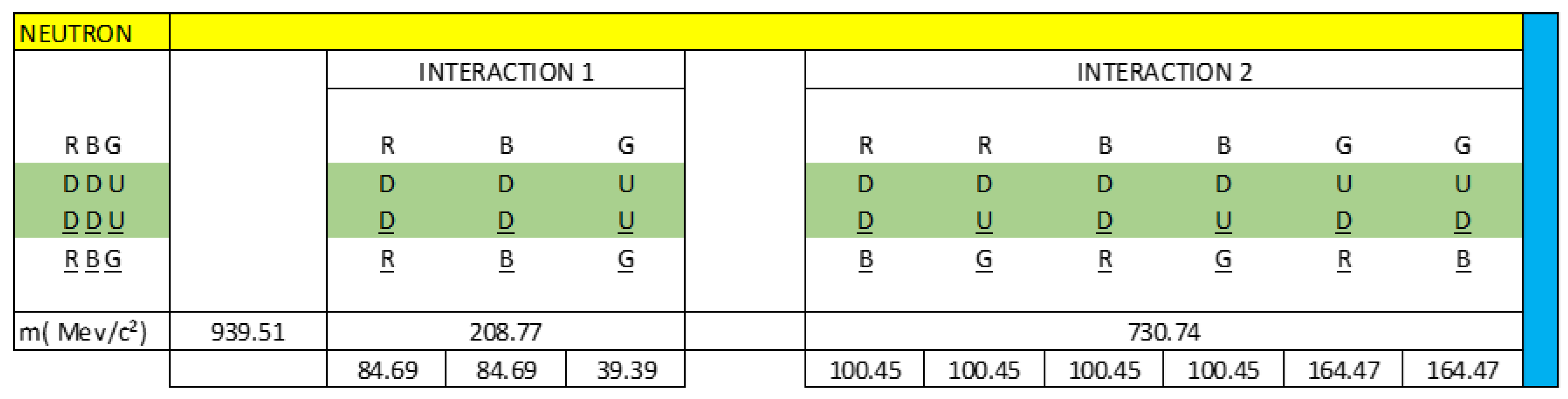
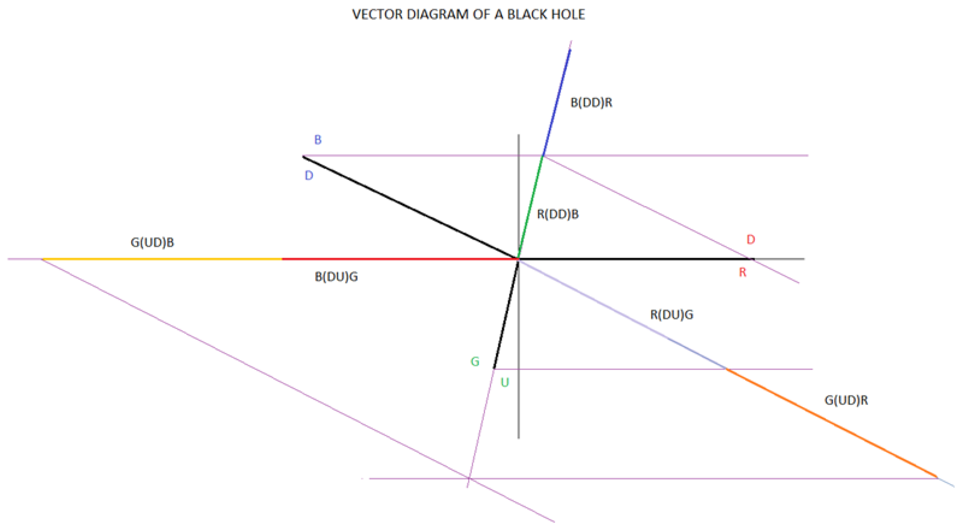
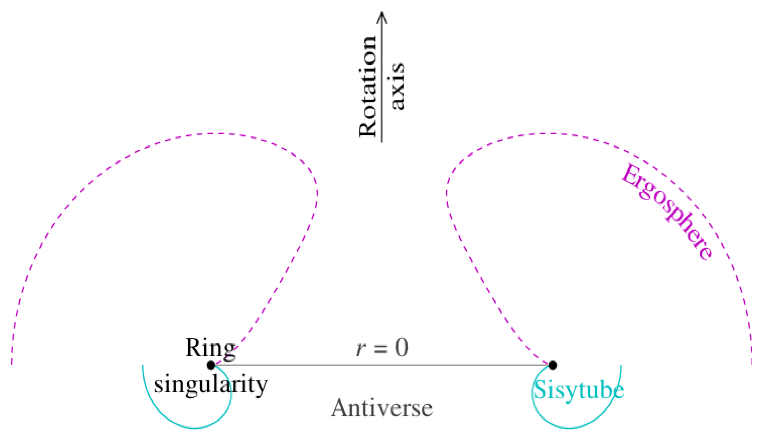
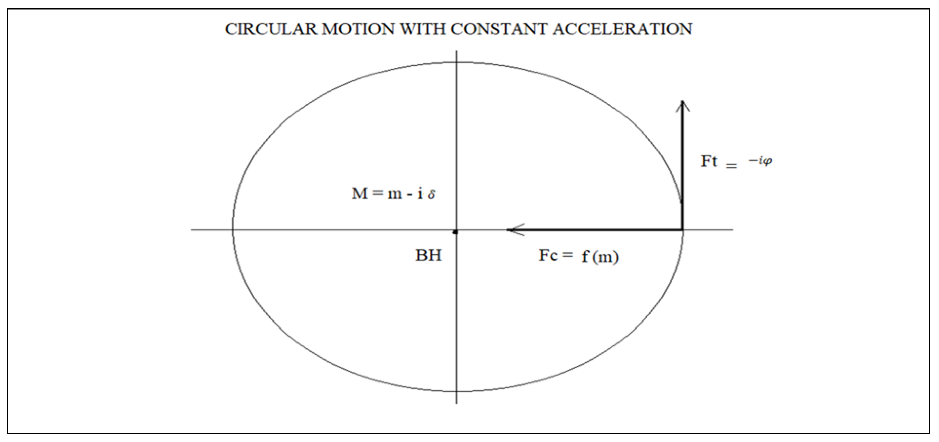
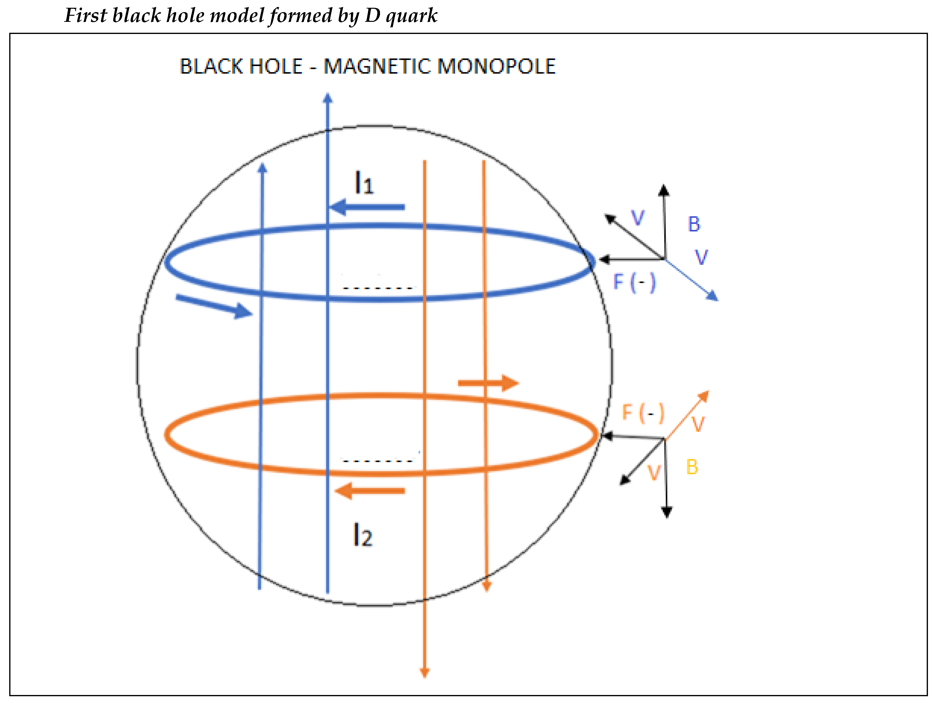
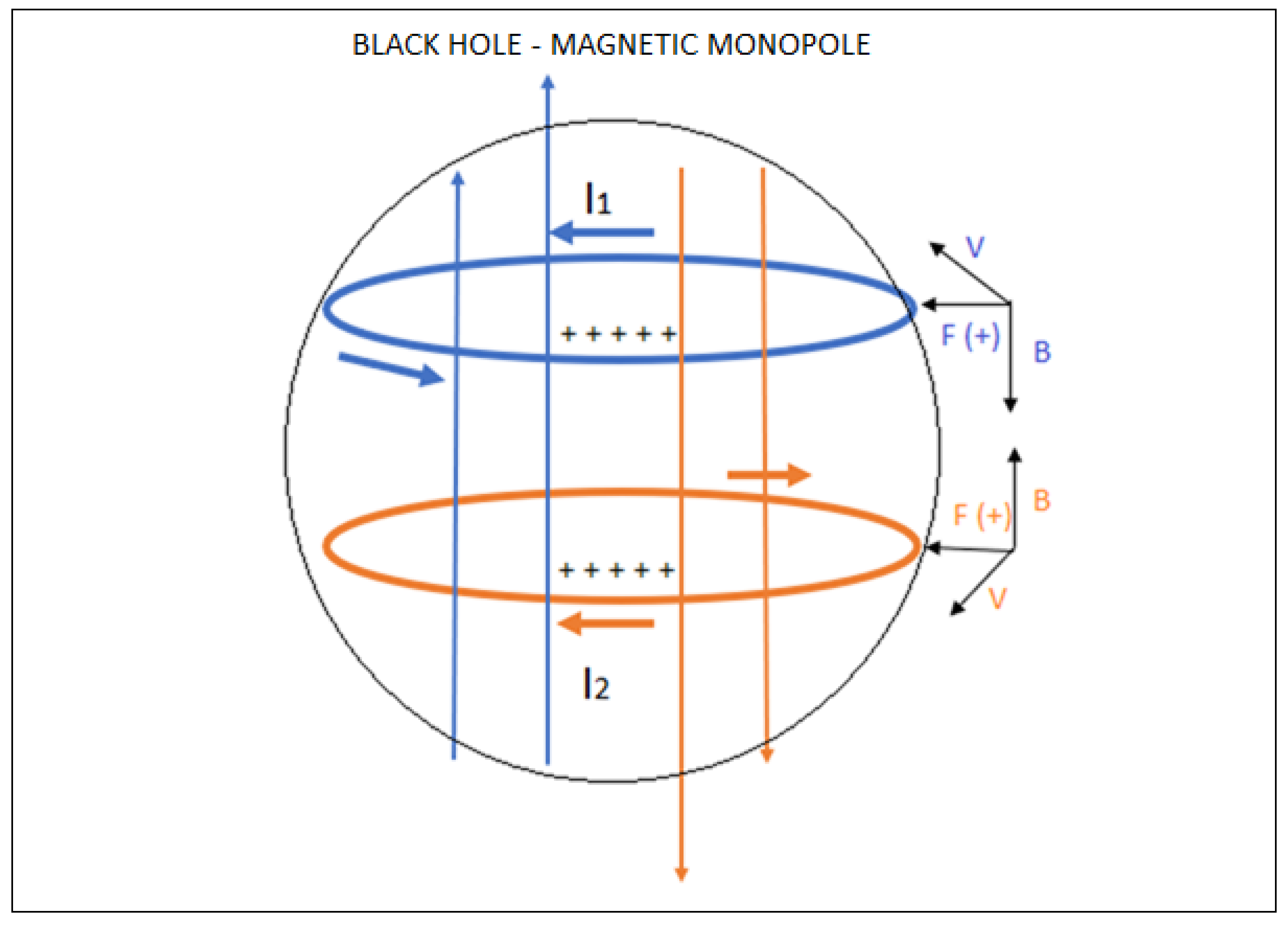
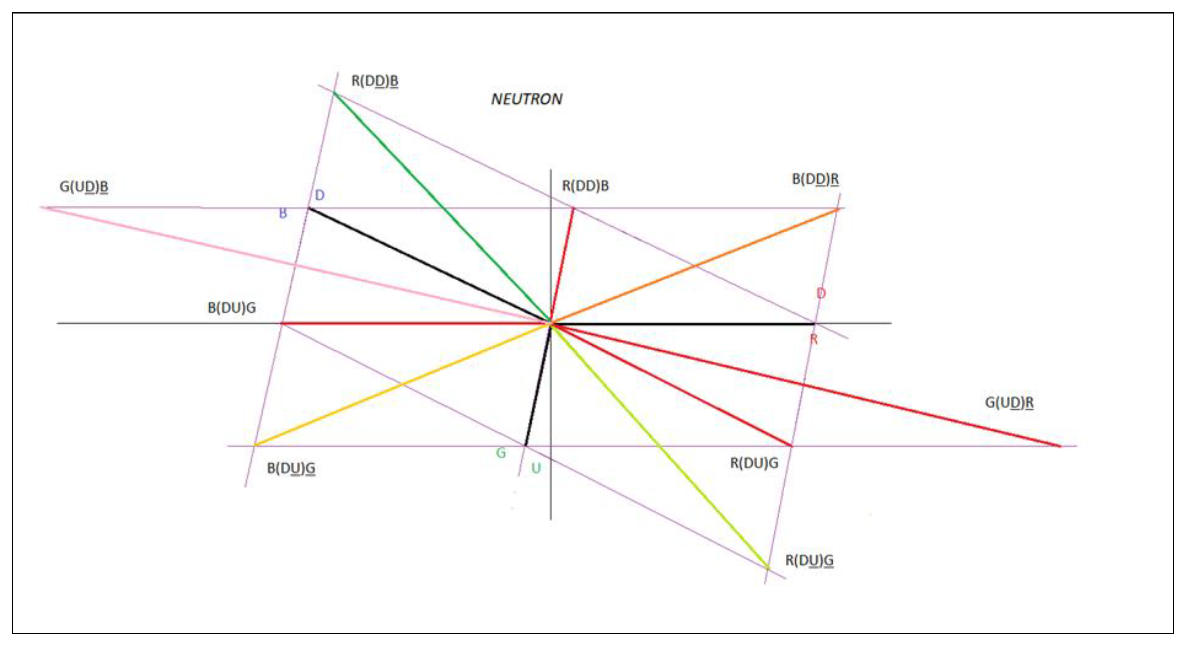
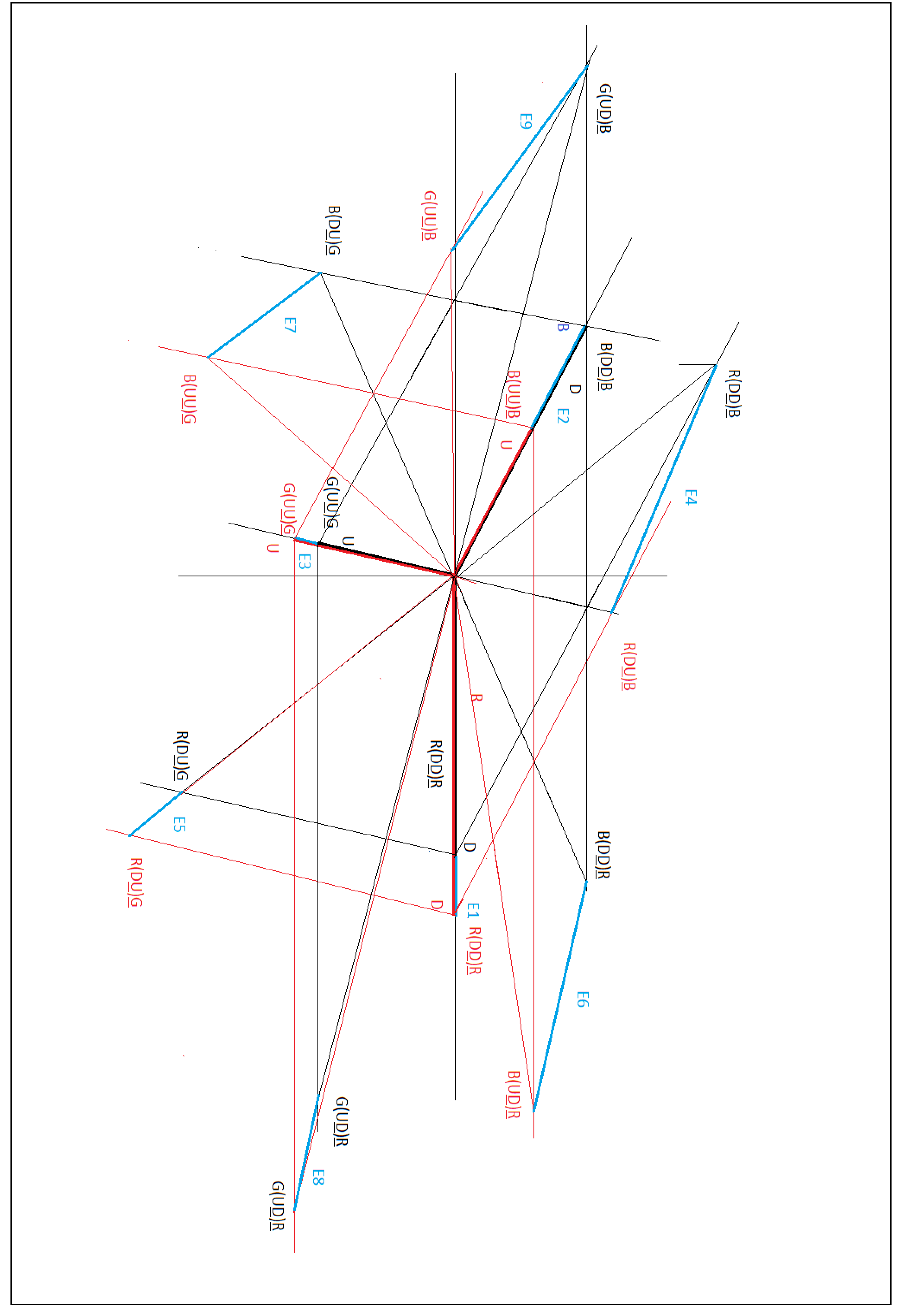
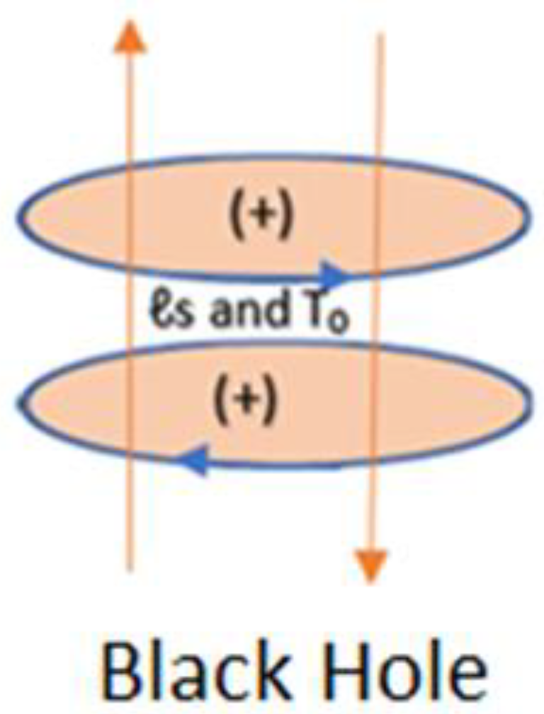
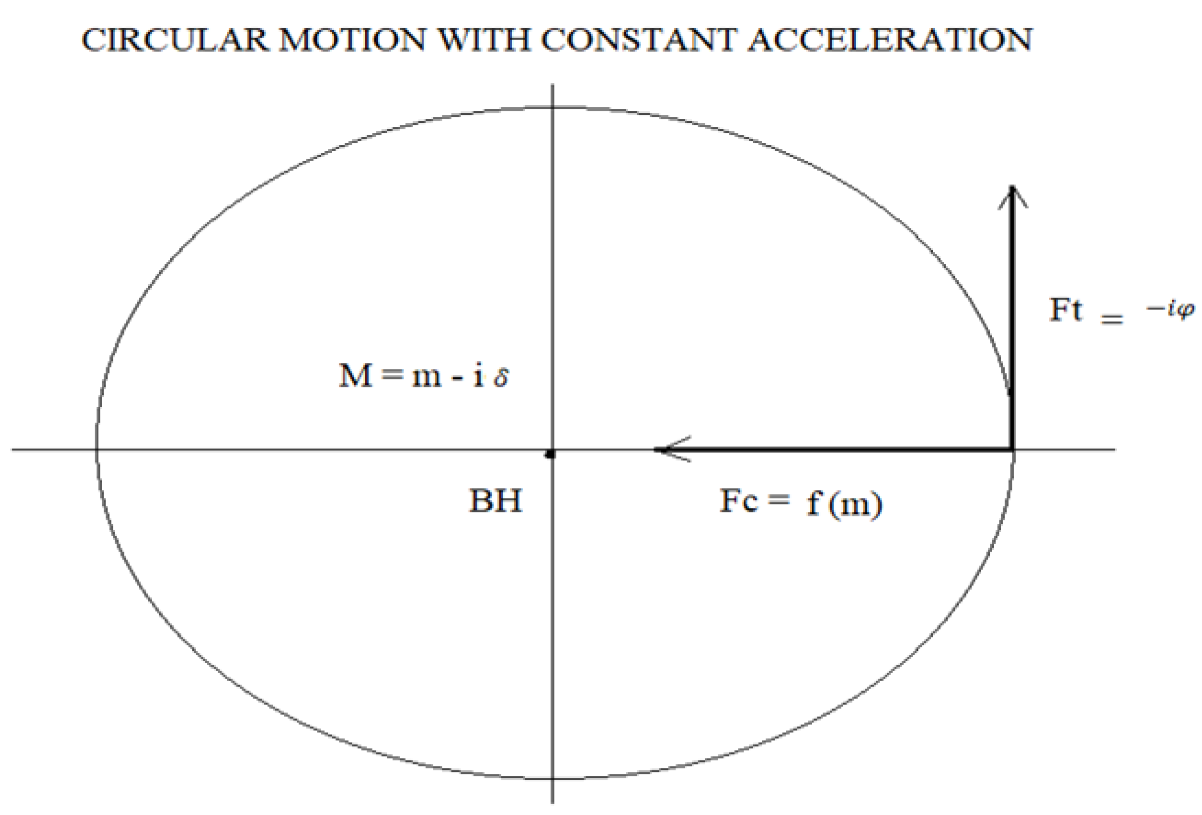
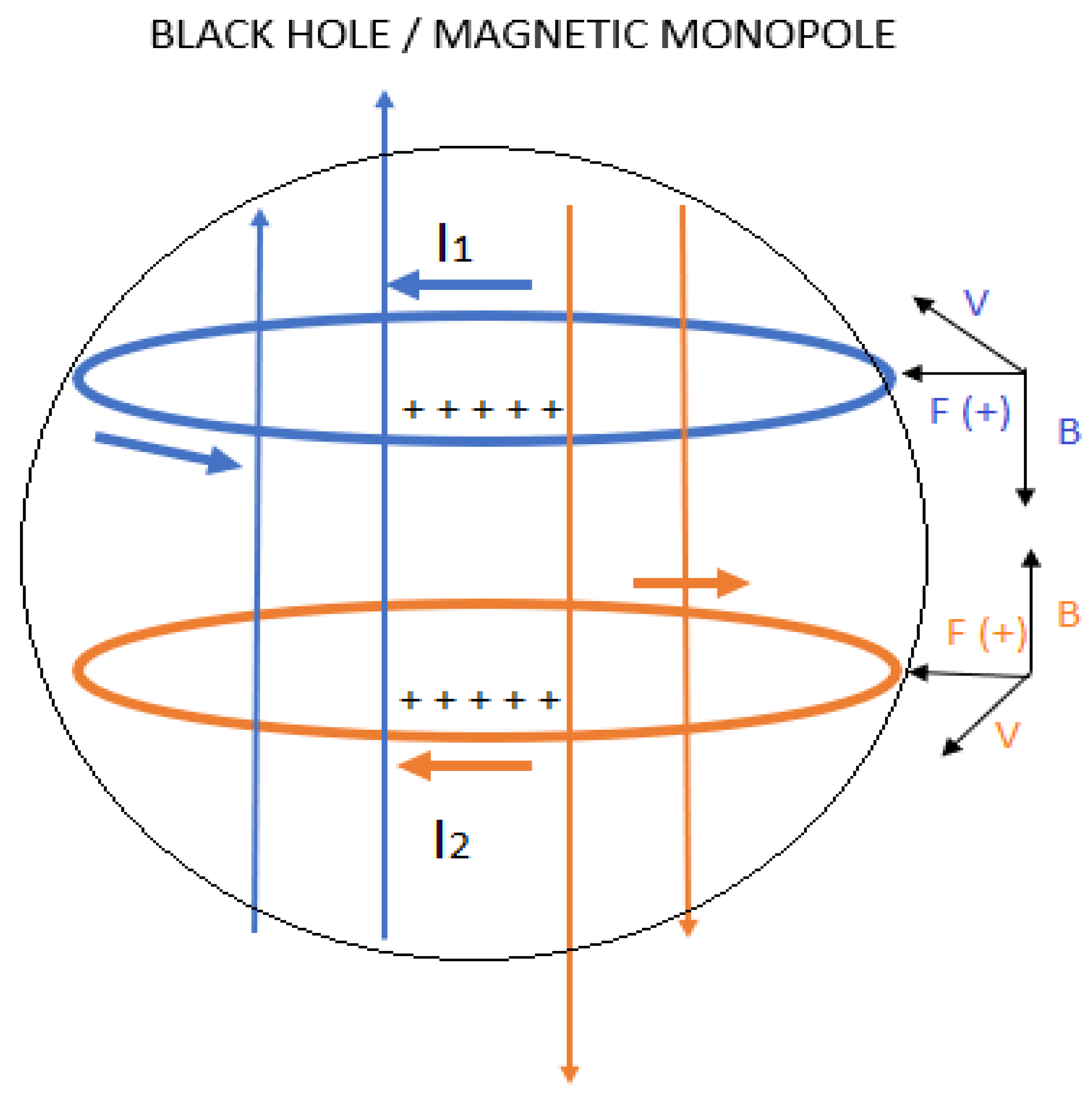
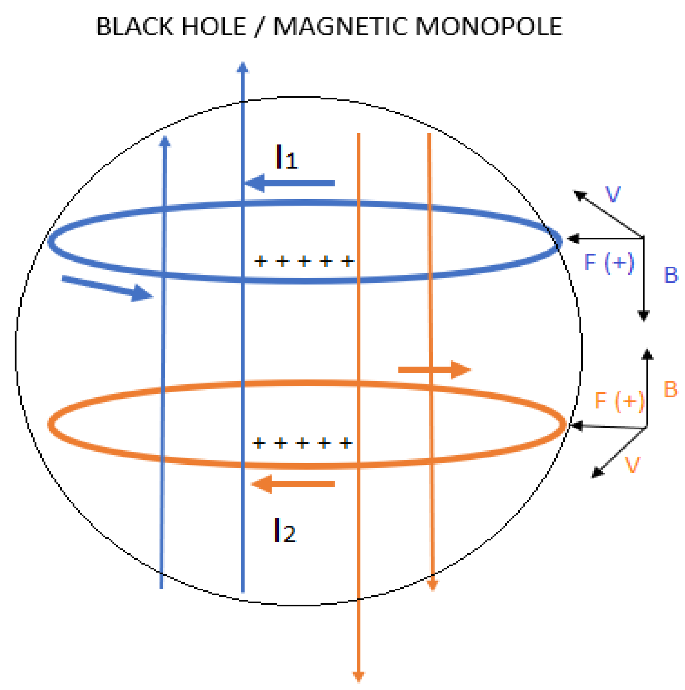
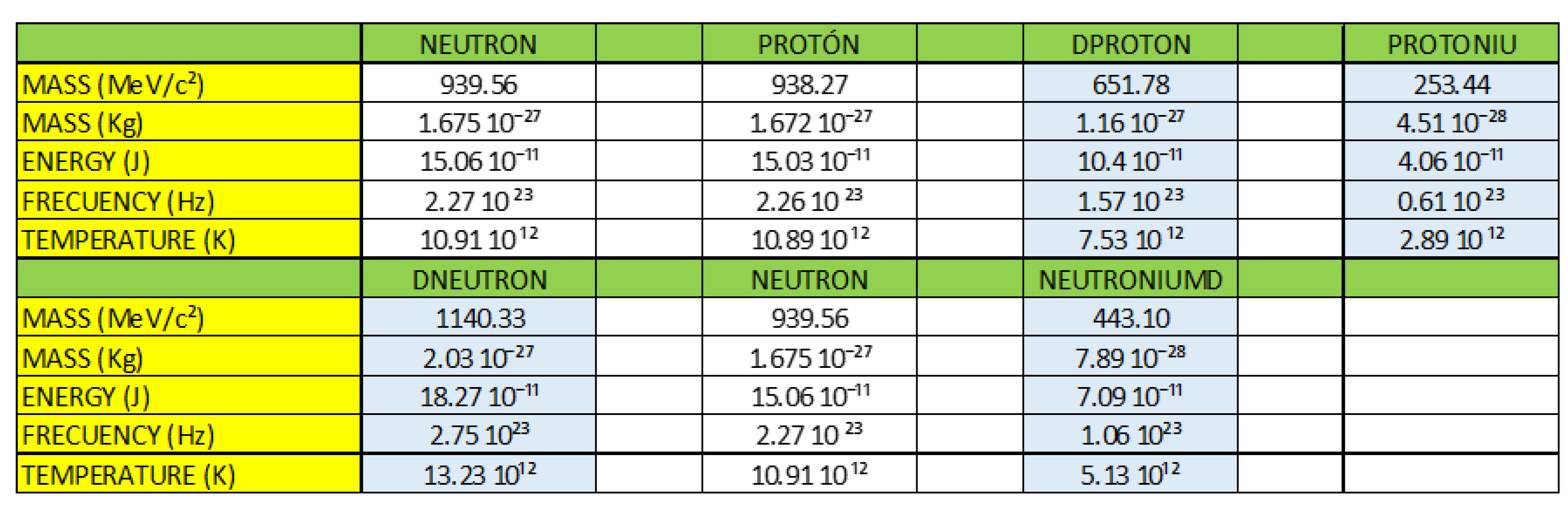
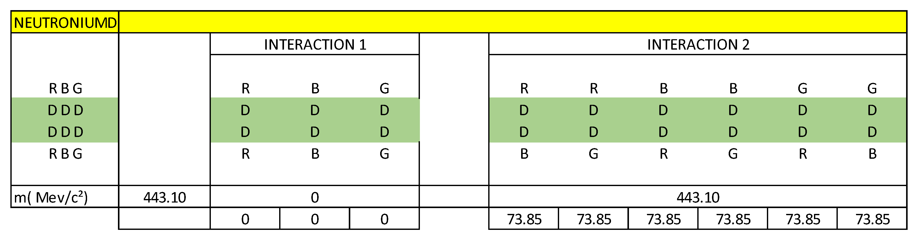
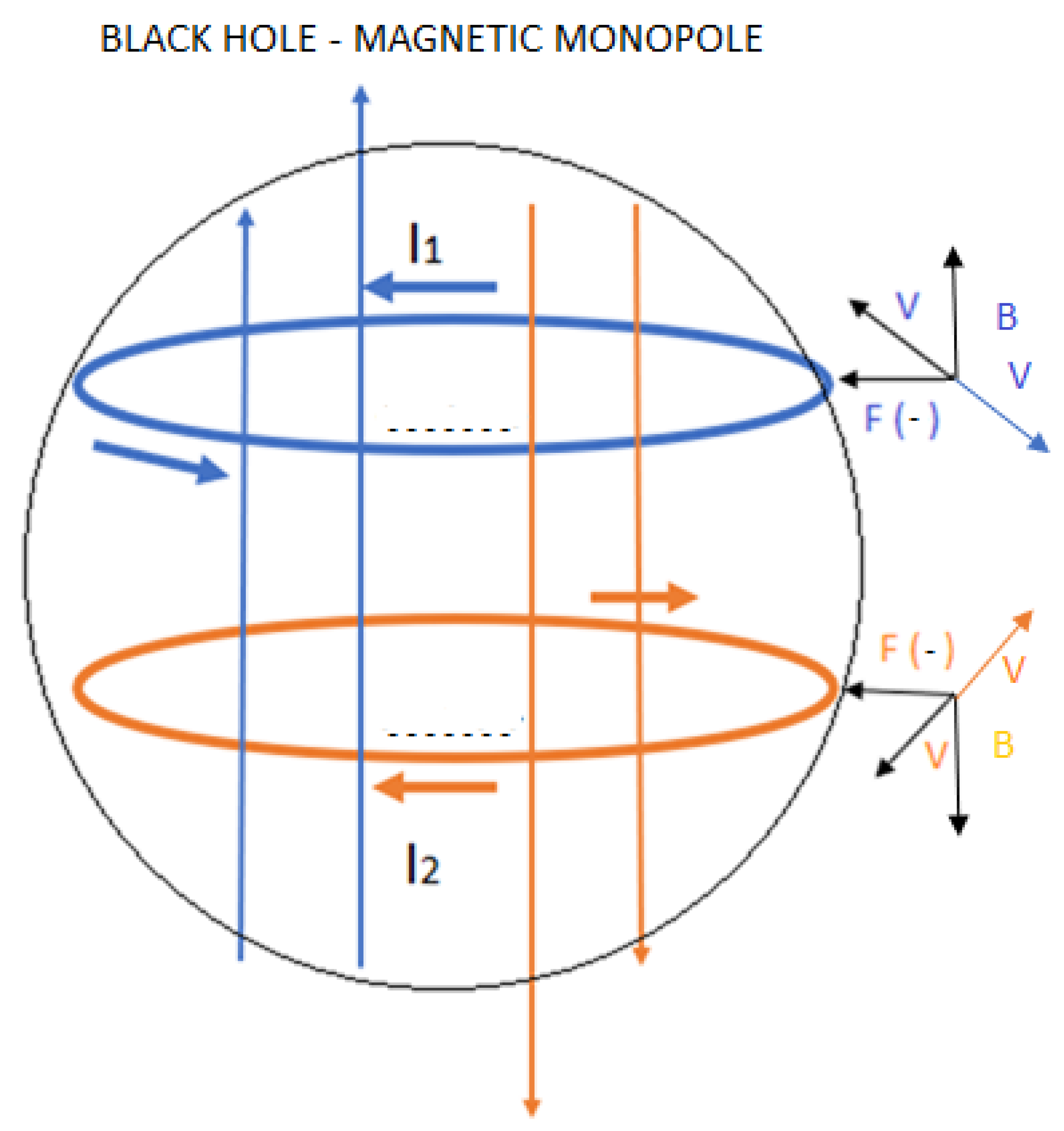
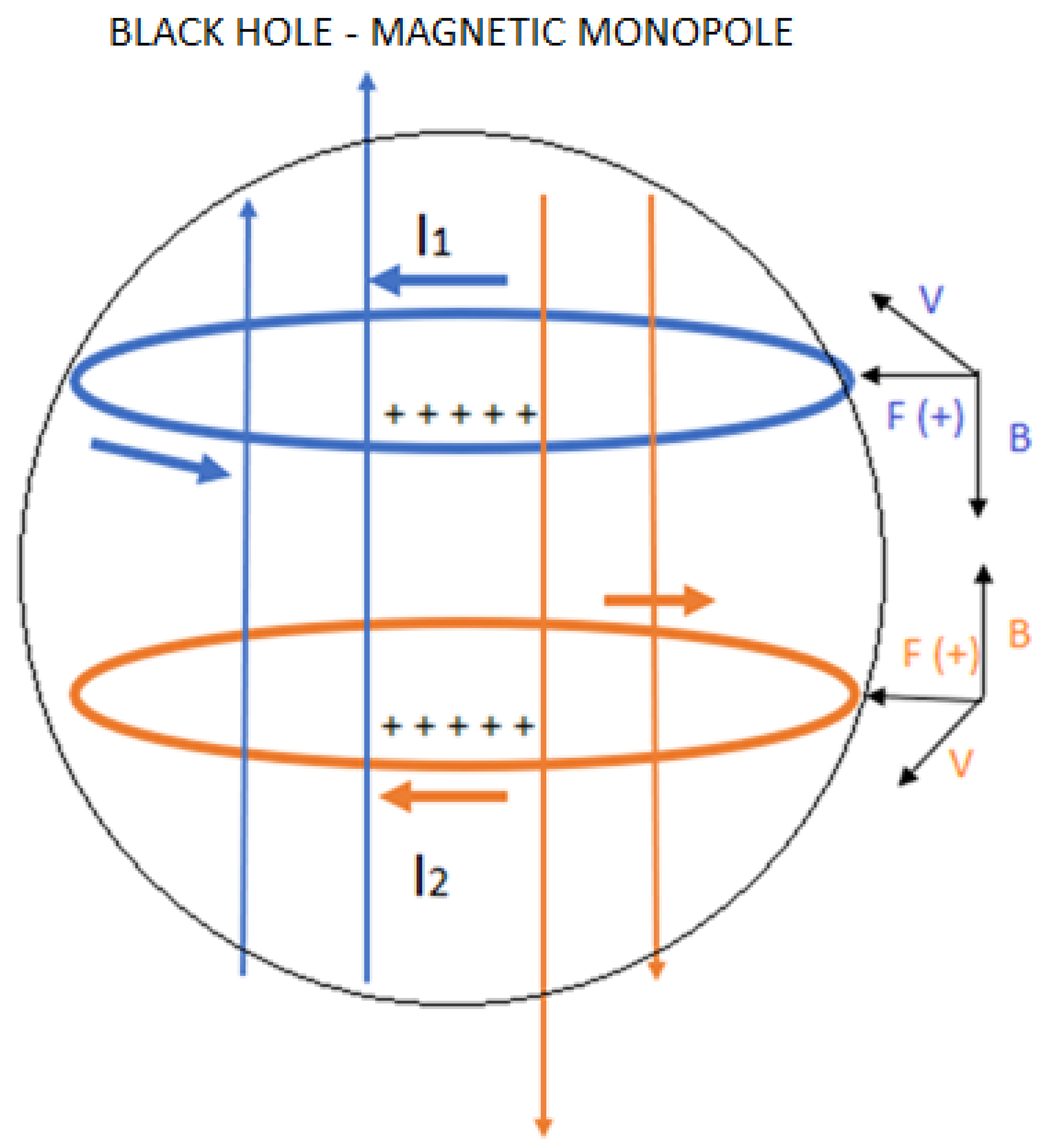
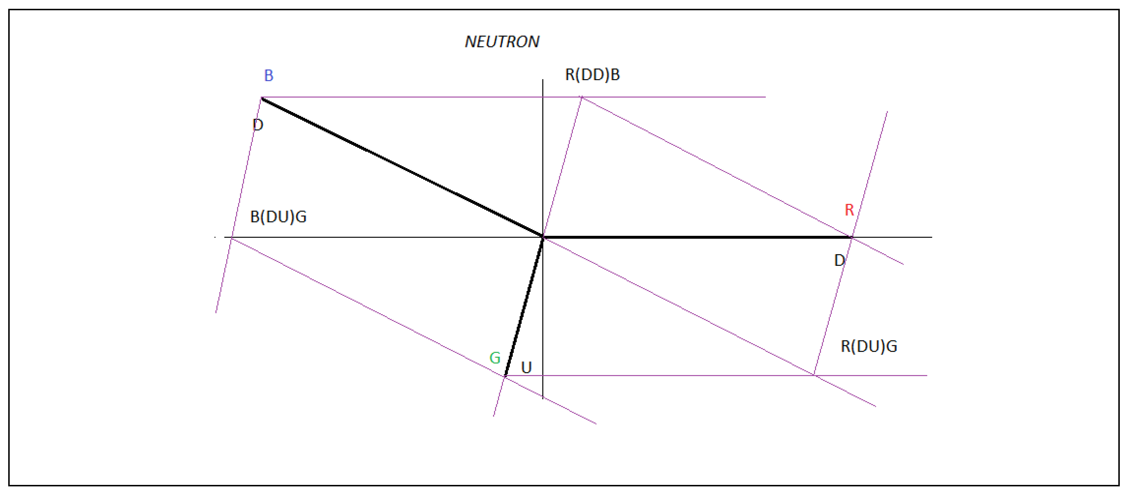
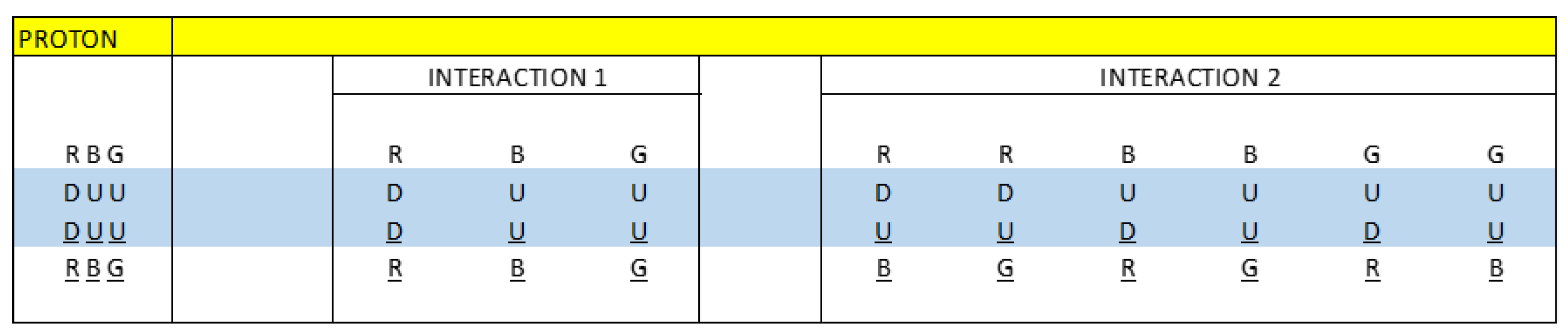
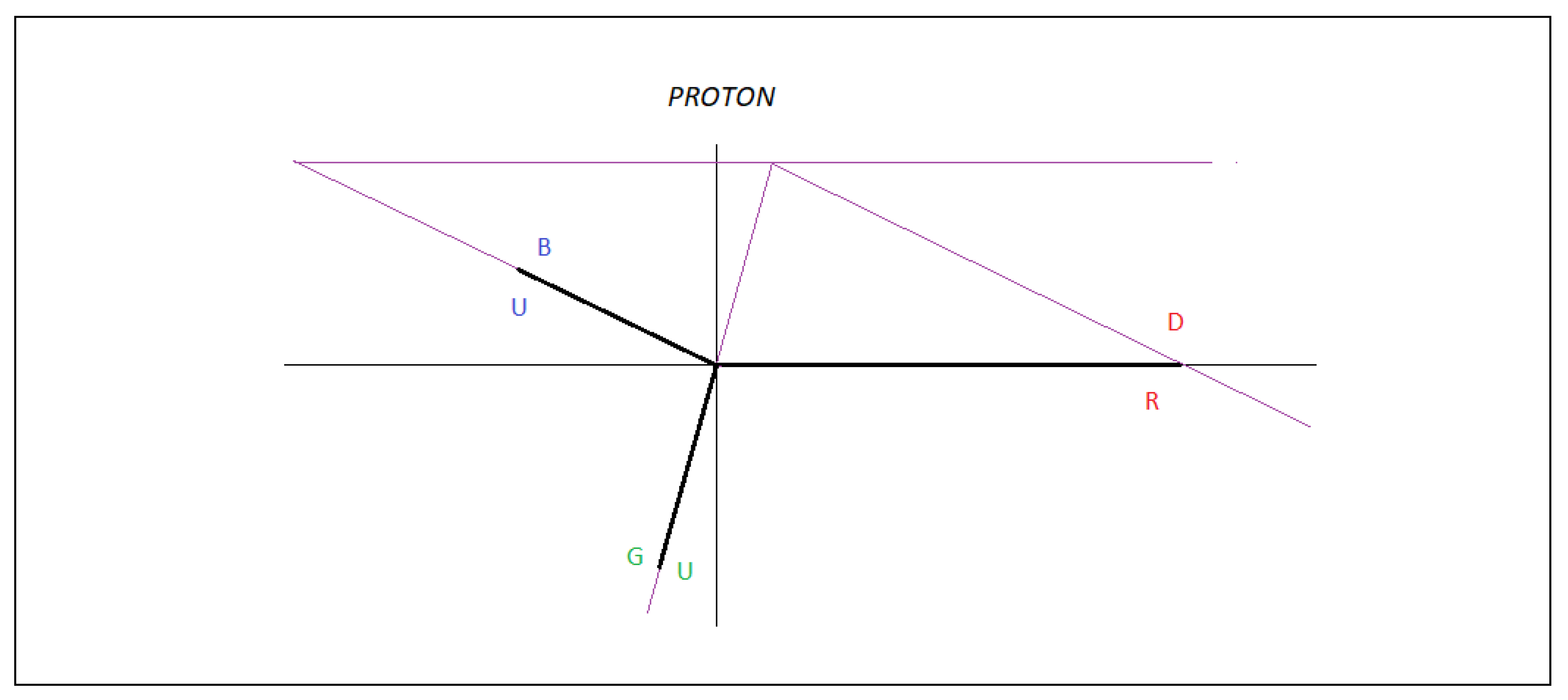
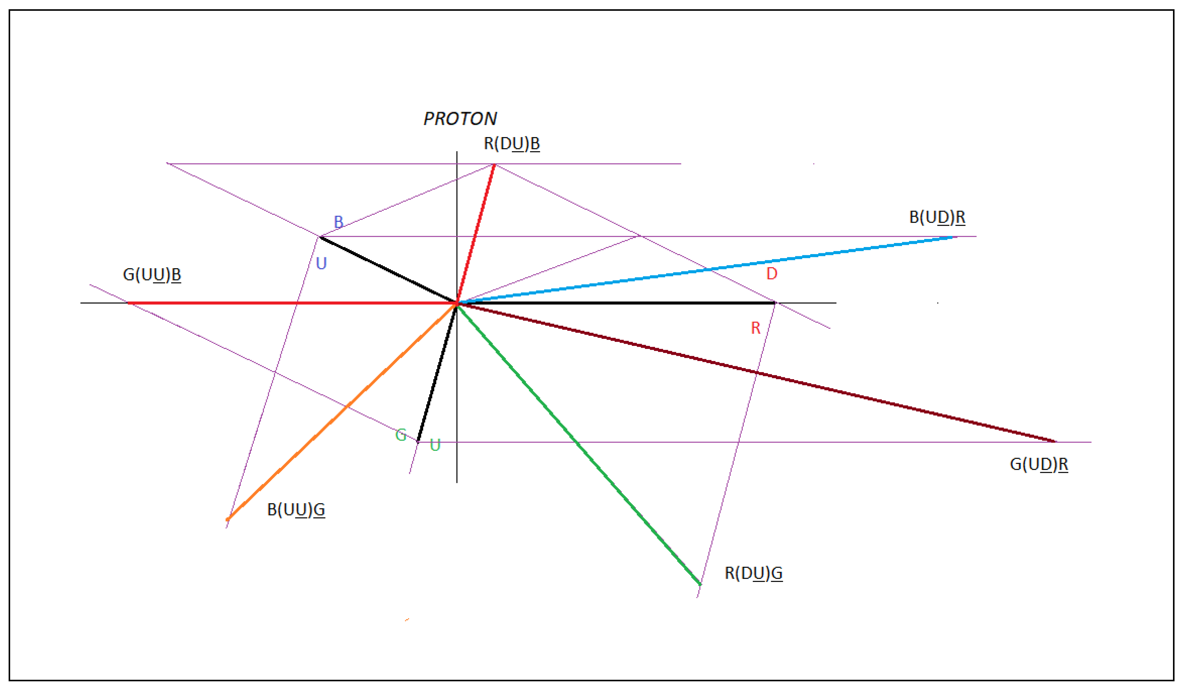
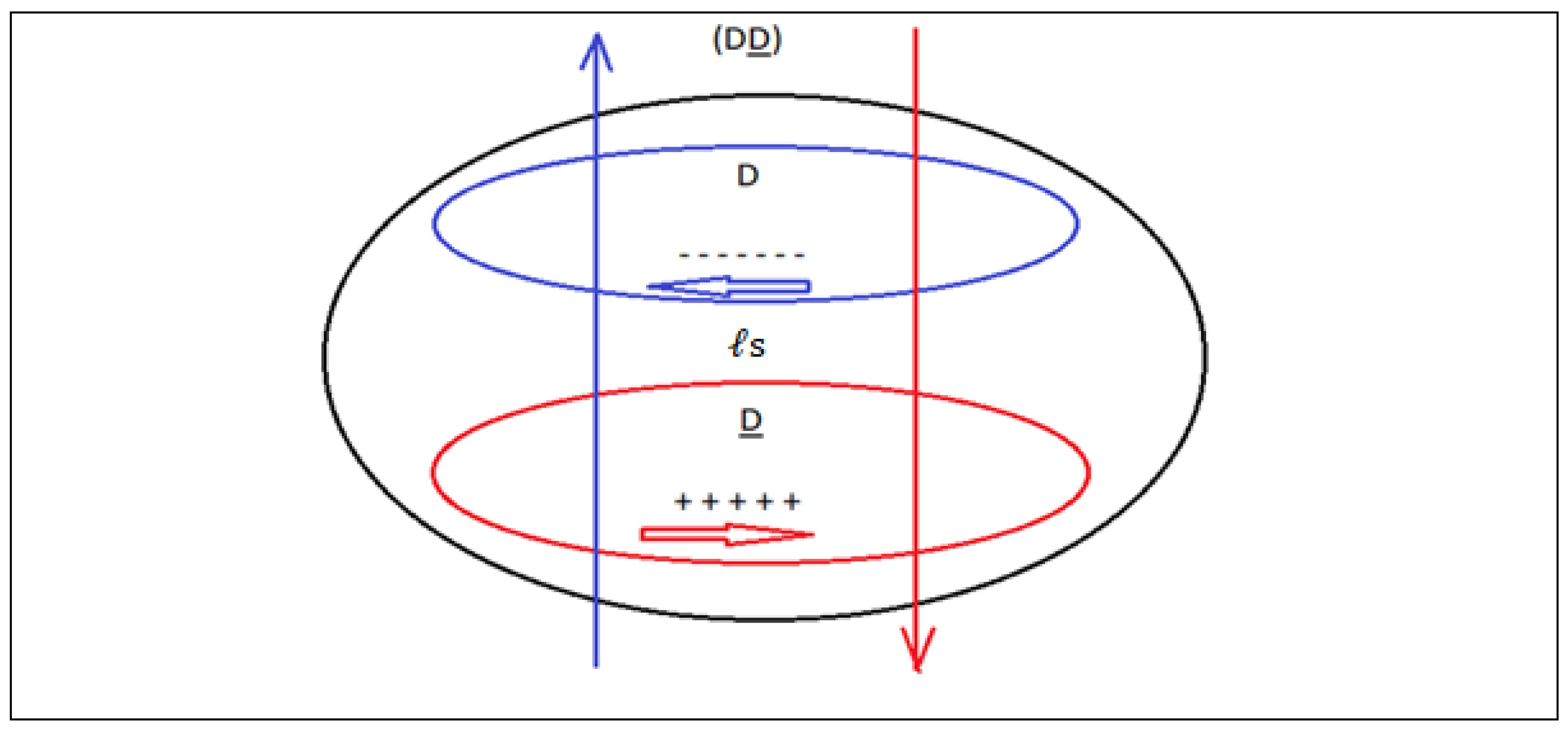
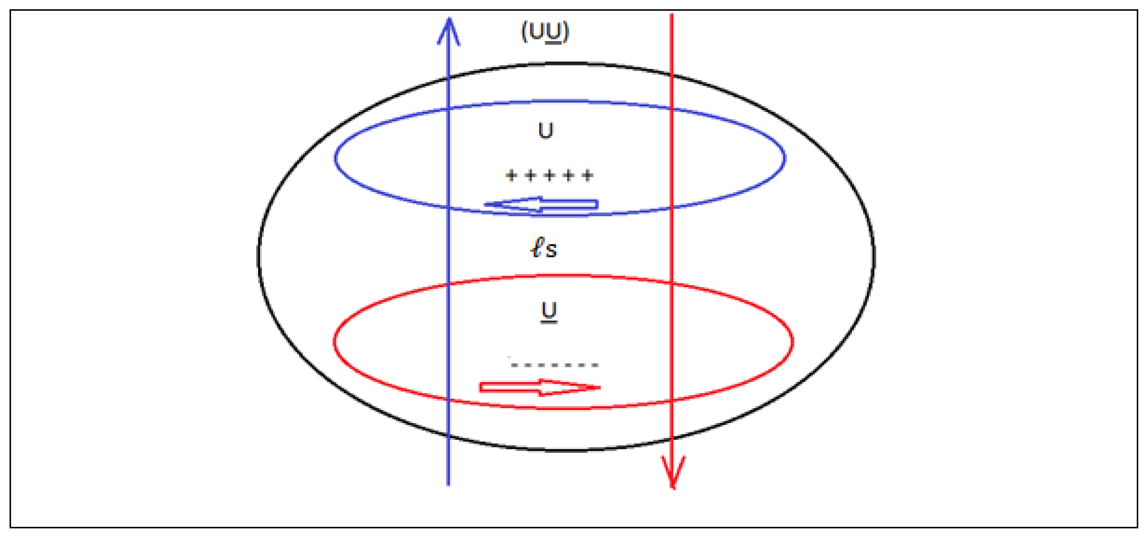
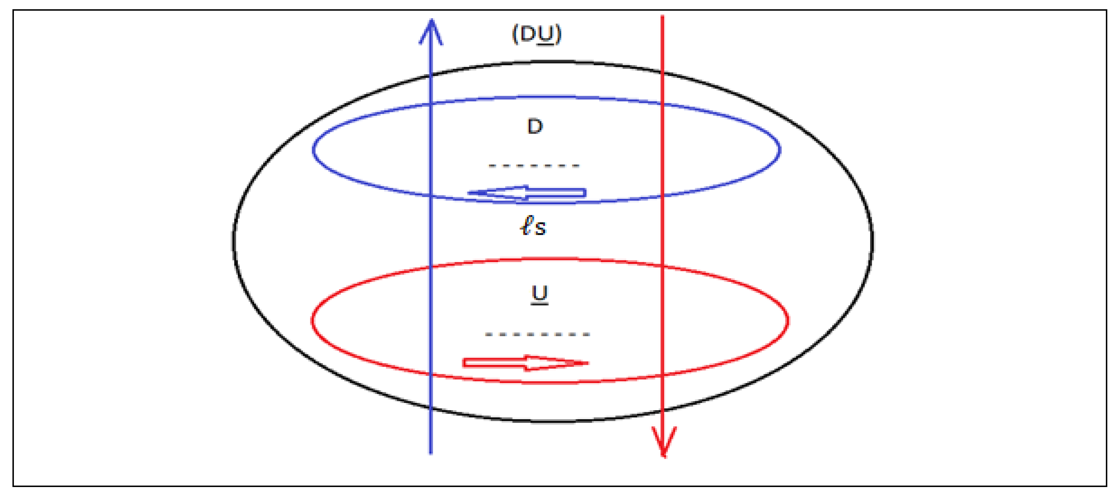
In the paper: Electrical-Quantum Modelling of the Neutron and Proton as a Three-Phase Alternating Current Electric Generator. Determination of the Number of Quarks-Antiquarks-Gluons and Gravitons, inside a Neutron; we proposed a model for black holes which we are going to represent in the following figure:
The explosion of a supernova goes beyond chemical energy or nuclear energy; that is why we propose that a supernova when it explodes separates matter and antimatter m (hw) from matter and antimatter m (-hw), in other words, the black hole that remains would be made up of matter and antimatter m (hw), m (-hw) expands in the space-time that surrounds the black hole.
With this we are proposing that inside a black hole there is no m (-hw), that is, the interior of a black hole is made up only of matter m (hw). This is represented in
Figure 107 and 108.
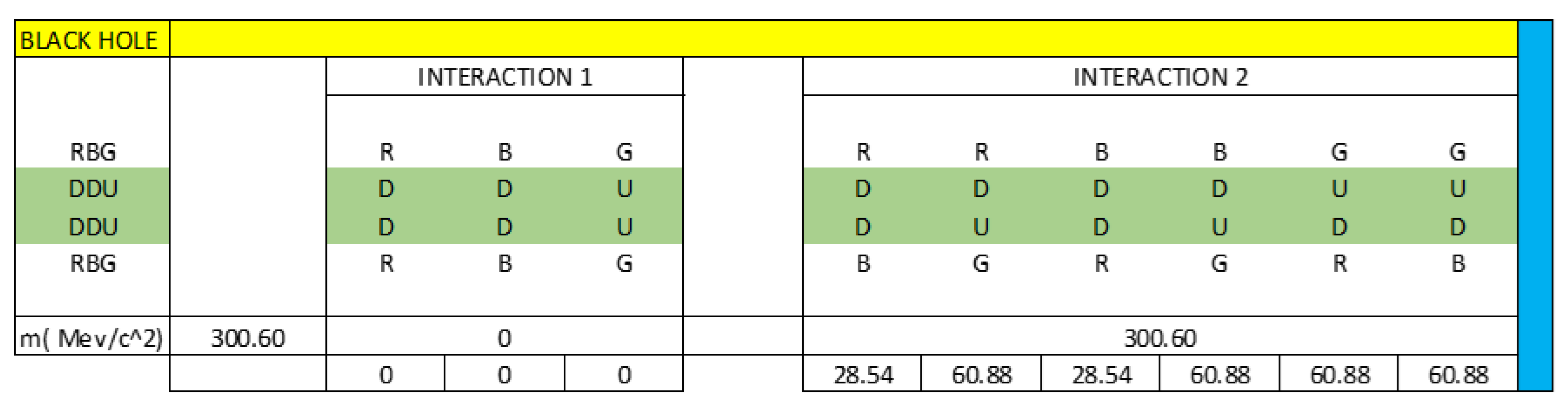
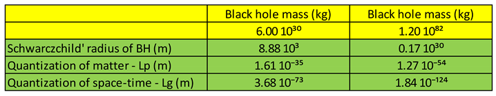
To conclude, let's consider the following table:
Conclusion:
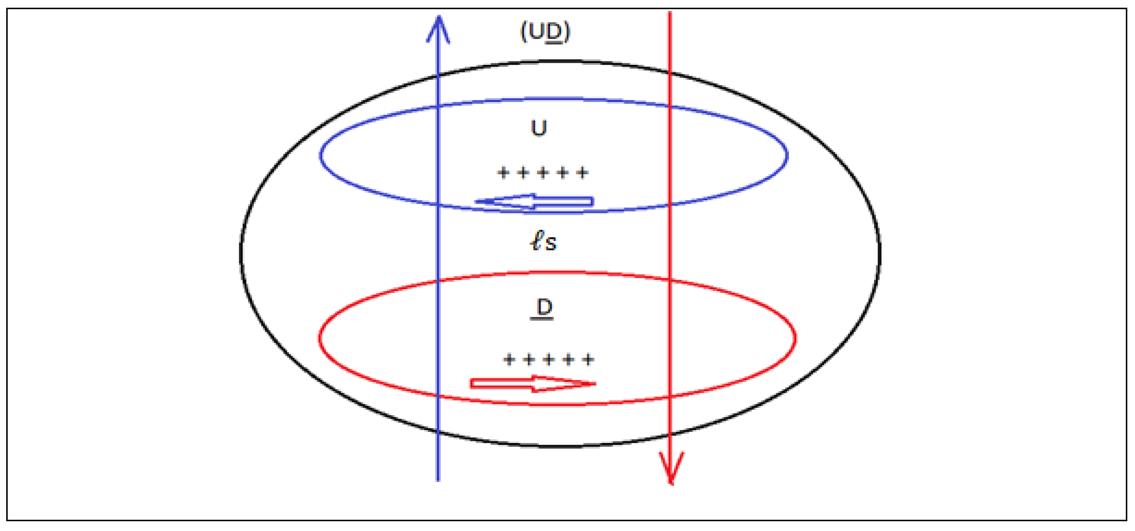
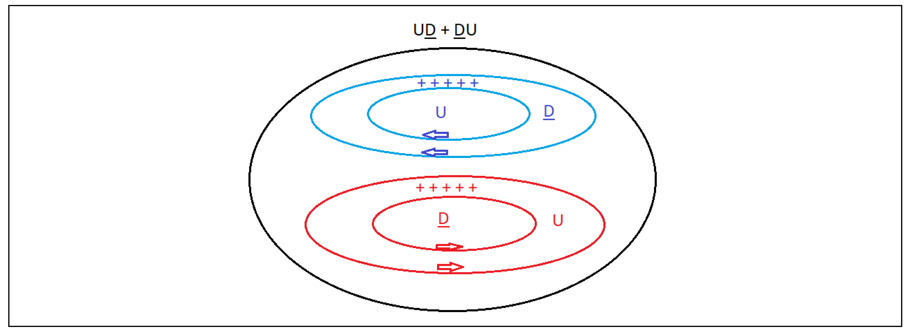
The ultra-dense Higgs field inside a black hole is not constant and varies between the following extremes:
H1 = 8.6 GeV (10¹³ K), minimum value of the ultra-dense Higgs field, occurs when a stellar black hole of three solar masses forms. See
Table 30.
H2 = 4.4 10¹⁵ GeV (5 10²⁶ K), maximum value of the ultra-dense Higgs field, is the value that the Higgs field takes inside a black hole at the moment T⁰, it explodes and produces a white hole or Big Bang. See
Table 30.
The ultra-dense state of the Higgs field varies between the values of H1 = 8.6 GeV (10¹³ K) < ultra-dense Higgs field < H2 = 4.4 10¹⁵ GeV (5 10²⁶ K); and only occurs inside black holes.
The first state of the Higgs field is associated with the false vacuum, domain of the four fundamental forces; the ultra-dense state of the Higgs field is associated with the true vacuum inside black hole, domain of the gravitational force field.
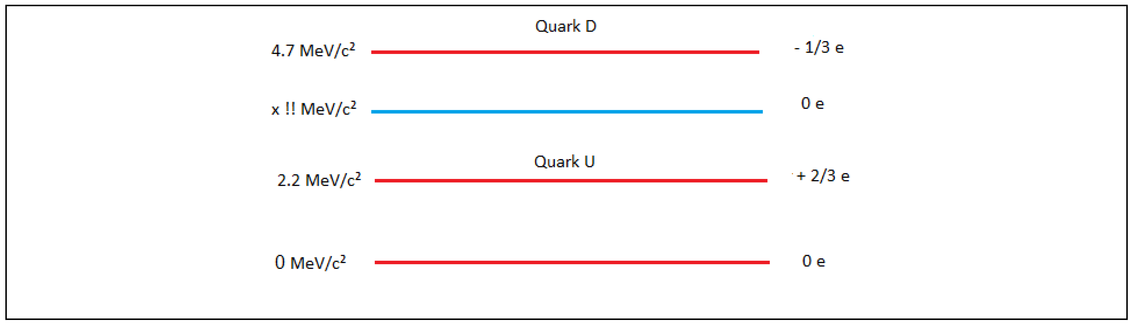
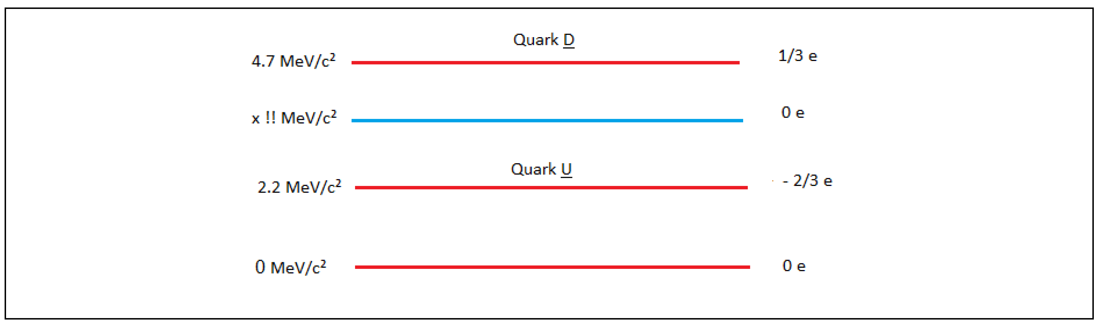
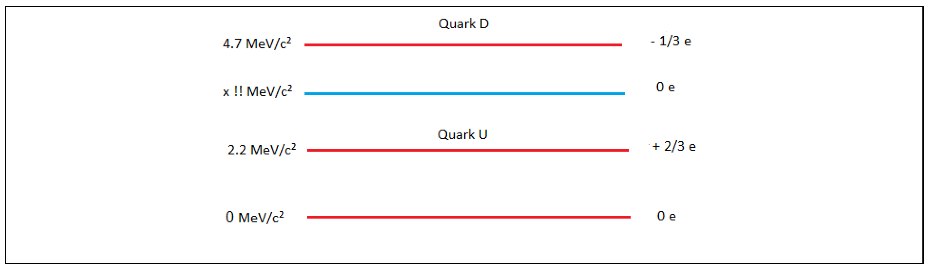
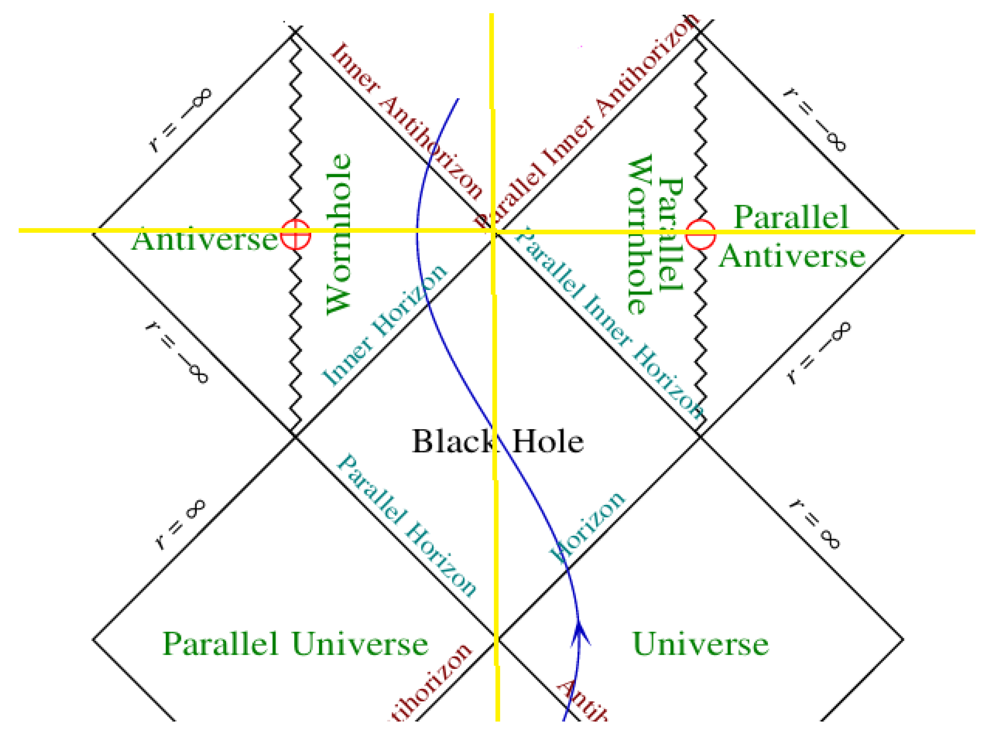
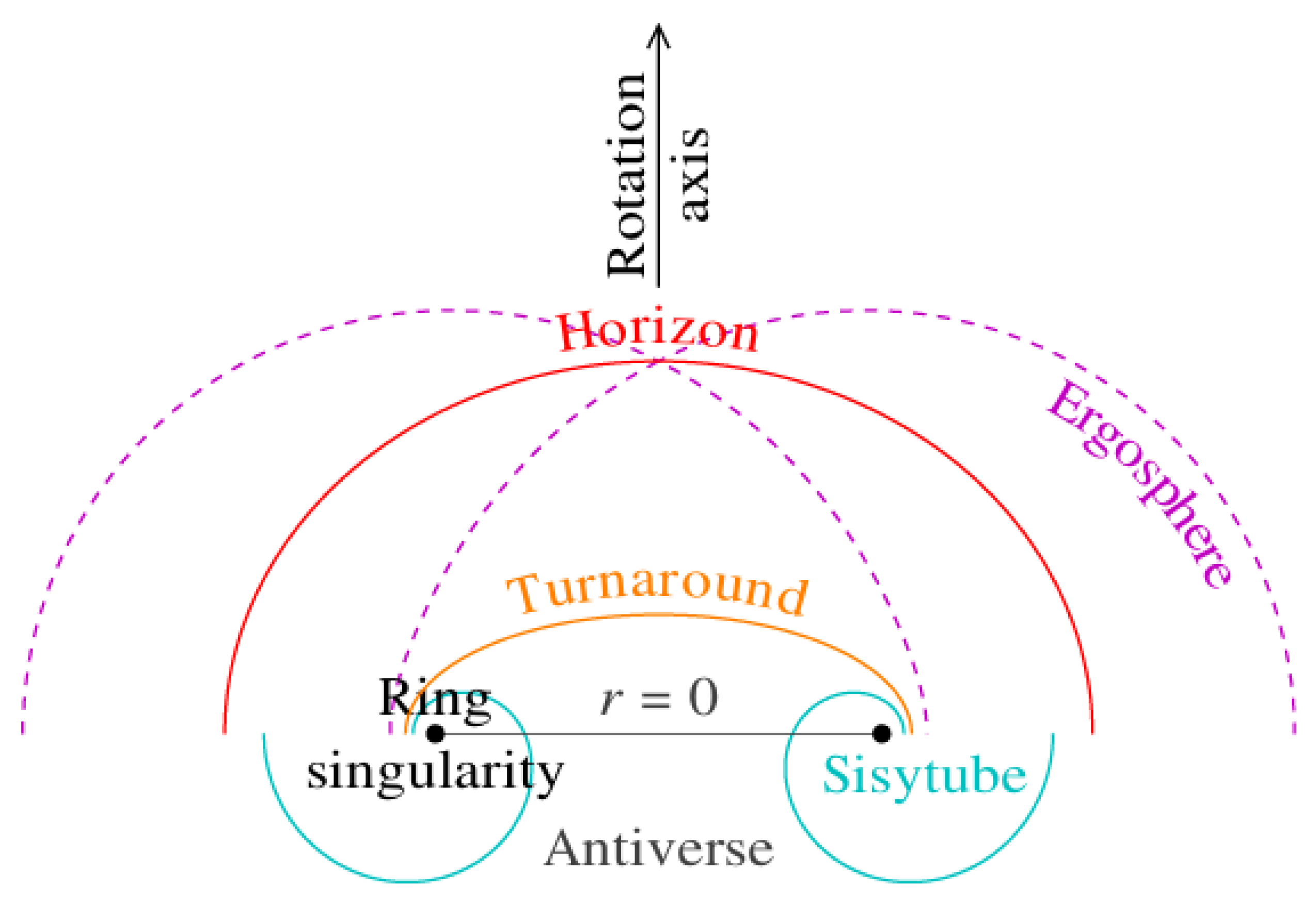
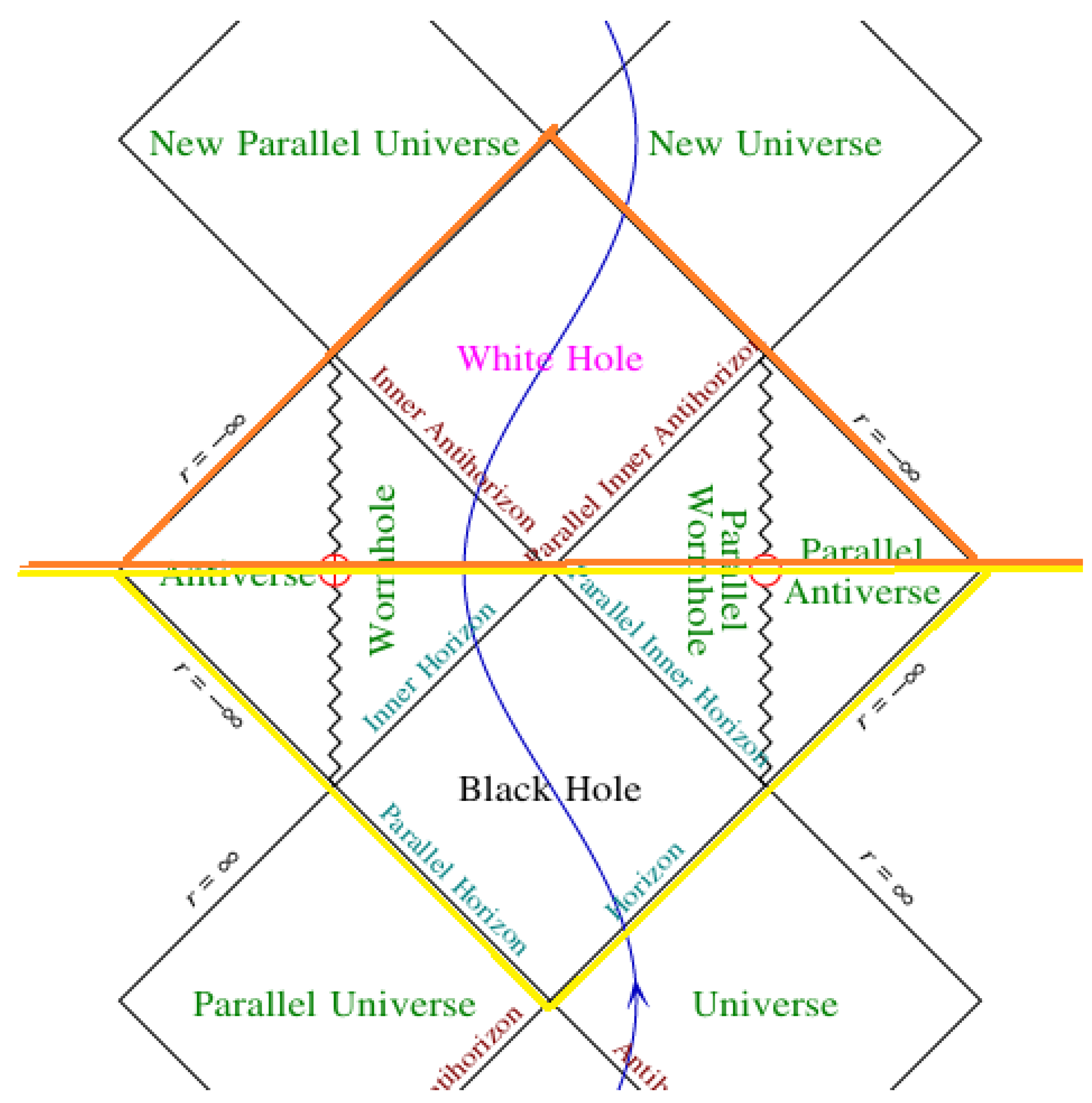
Figure 109.
The two states of the Higgs field.
Figure 109.
The two states of the Higgs field.
Example 4:
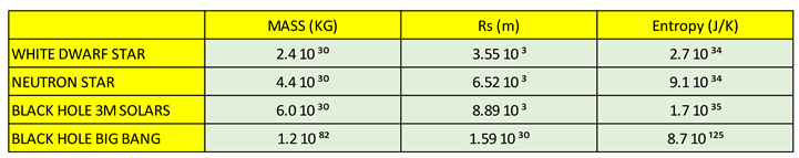
Calculation of the entropy of a black hole, neutron star and white dwarf star
To perform entropy calculations for stellar bodies such as white dwarf stars and neutron stars or possibly any stellar body, we will first calculate the equivalent black hole of the body of interest and then using the entropy formula of a black hole, we will calculate the entropy value for that body in question; as a final result, the entropy of the body of interest will be less than or equal to the entropy of its counterpart black hole. Using this mechanism, we can estimate the approximate entropy value of any stellar body knowing that it cannot be greater than the entropy of its equivalent black hole.
We will calculate the entropy value for the following situations:
A) Calculation of the entropy of a black hole of three solar masses.
B) Calculation of the entropy of a black hole at the moment of the Big Bang.
C) Calculation of entropy for a neutron star.
D) Calculation of entropy for a white dwarf star.
We are going to use the following entropy equations:
S = (4 π Kʙ-eff G² M²) / Lp²C⁴ (132)
S = (π Kʙ-eff Rs²) / Lp² (133)
Kʙ-eff = effective Boltzmann´s constant, G = Universal gravitational constant, M = mass of a body to calculate entropy, Lp = Planck length, C = Speed of light and Rs = Schwarzschild radius.
Comments:
When applying the formula to calculate the entropy of a black hole, it is important to clarify that the Boltzmann´s constant used corresponds to the Boltzmann´s constant of a black hole and assumes the following value, Kʙ = 1.78 10⁻⁴³ J/K.
A) Calculation of the entropy of a black hole of three solar masses
M = 3ϴ = 6 10³⁰ kg
Kʙ-eff = 1.78 10⁻⁴³ J/K
C = 3 10⁸ m/s
Lp = 1.61 10⁻³⁵ m
S = (4 π Kʙ-eff G² M²) / Lp² C⁴
Replacing the values,
S = 4 x 3.14 x 1.78 10⁻⁴³ x 36 10⁶⁰ x 44.48 10⁻²² / (2.59 10⁻⁷⁰ x 81 10³²)
S = 35799.49 10⁻⁵ / 209.79 10⁻³⁸
S = 1.70 10³⁵ J/K
B) Calculation of the entropy of a black hole at the moment of the Big Bang
M = 1.20 10⁸² kg
Kʙ-eff = 1.78 10⁻⁴³ j/k
C = 3 10²¹ m/s
Lp = 1.27 10⁻⁵⁴ m
Rs = 1.59 10³⁰ m
S = 4 π Kʙ G² M² / (Lp² C⁴)
Replacing the values,
S = 4 x 3.14 x 1.78 10⁻⁴³ x 1.44 10¹⁶⁴ x 44.48 10⁻²² / (1.61 10⁻¹⁰⁸ x 81 10⁸⁴)
S = 1431.97 10⁹⁹ / 130.41 10⁻²⁴
S = 1.098 10¹²⁴ J/K
S = π Kʙ x Rs² / Lp²
S = 3.14 x 1.78 10⁻⁴³ x 2.52 10⁶⁰ / 1.61 10⁻¹⁰⁸
S = 14.08 10¹⁷ / 1.61 10⁻¹⁰⁸
S = 8.74 10¹²⁵ J/K
C) Calculation of entropy for a neutron star
M = 2.2Mϴ = 4.4 10³⁰ kg
Calculation of the Schwarzschild´s radius.
Rs = 2 G M/C²
Rs = 2 x 6.67 10⁻¹¹ x 4.4 10³⁰ / 9 10¹⁶ = 58.69 10³⁰ / 9 10¹⁶ = 6.52 10³ m
Rs = 6.52 10³ m
Entropy calculation:
S = π Kʙ-eff Rs² / Lp²
S = 3.14 x 1.78 10⁻⁴³ x 42.51 10⁶ / 2.59 10⁻⁷⁰
S = 237.59 10⁻³⁷ / 2.59 10⁻⁷⁰
S = 9.173 10³⁴ J/K
D) Calculation of entropy for a white dwarf star
M = 1.2 Mϴ = 2.4 10³⁰ kg
Calculation of the Schwarzschild´s radius:
Rs = (2 G M) / C²
Rs = 2 x 6.67 10⁻¹¹ x 2.4 10³⁰ / 9 10¹⁶ = 32.016 10³⁰ / 9 10¹⁶ = 3.55 10³ m
Rs = 3.55 10³ m
Entropy calculation:
S = π Kʙ-eff Rs² / Lp²
S = 3.14 x 1.78 10⁻⁴³ x 12.60 10⁶ / 2.59 10⁻⁷⁰
S = 70.43 10⁻³⁷ / 2.59 10⁻⁷⁰
S = 2.719 10³⁴ J/K
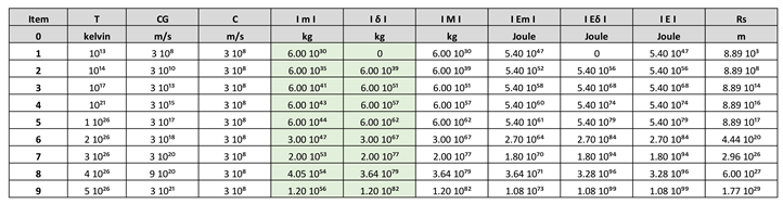
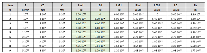
Finally, in
Table 31, we will represent a summary of the entropy calculations for different stellar bodies.
Example 5:
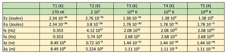
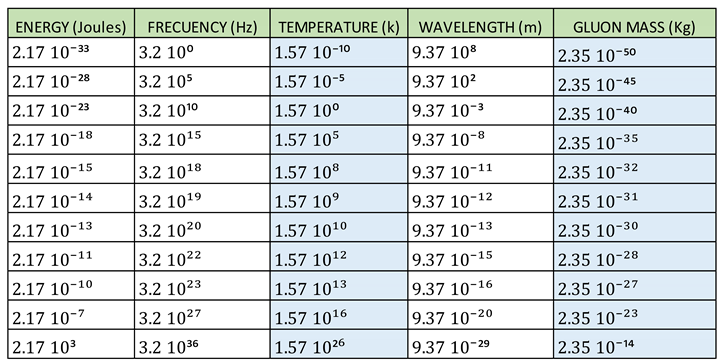
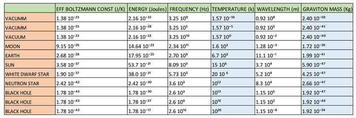
Analysis of the equations of the electromagnetic and gravitational wave spectrum
We will describe simple equations that represent the electromagnetic wave spectrum.
Eε = h x fε
Cε = λε x fε
Eε = h x Cε / λε
Eε = Kʙε x Tε
Kʙε = 1.38 10⁻²³ J/K
We will describe simple equations that represent the gravitational wave spectrum.
Eɢ = h x fɢ
Cɢ = λɢ x fɢ
Eɢ = h x Cɢ / λɢ
Eɢ = Kʙɢ x Tɢ
Kʙɢ = 1.38 10⁻²³ J/K > Kв-eff > 1.78 10⁻⁴³ J/K
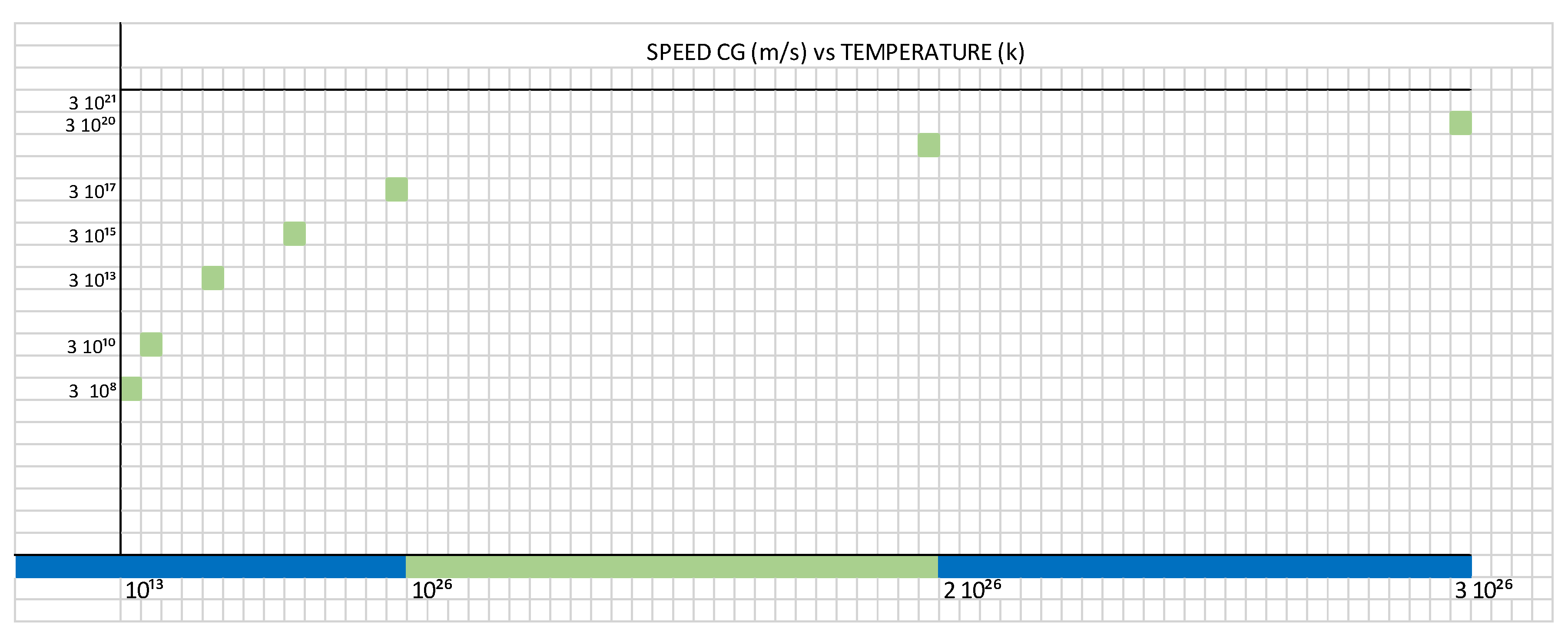
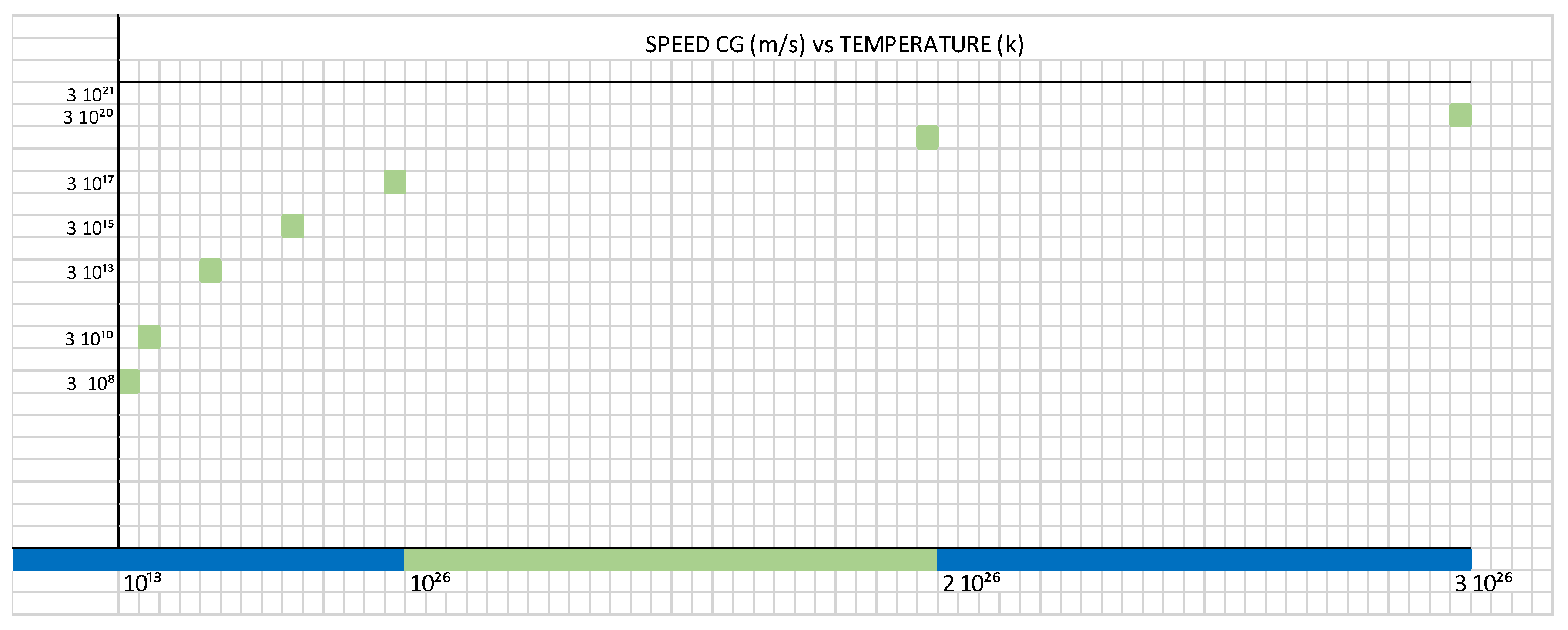
We are going to carry out our analysis from the point of view of temperature, we are going to consider the following equations:
Eε = Kʙε x Tε (134)
Eɢ = Kʙɢ x Tɢ (135)
- i)
T = 170 nK, temperature of the Bose-Einstein condensate for Rubidium atoms.
Eε = Kʙε x Tε
Eε = Kʙε x Tε = 1.38 10⁻²³ J/K x 170 10⁻⁹ K = 234.6 10⁻³² = 2.34 10⁻³⁴ J
Eε = 2.34 10⁻³⁴ J
Eε = h x fε
fε = Eε / h = 2.34 10⁻³⁴ J / 6.62 10⁻³⁴ = 0.353
fε = 0.353 Hz
C = λε x fε
λε = C / fε = 3 10⁸ / 0.353 = 8.49 10⁸ m
Eɢ = Kʙɢ x Tɢ
Eɢ = Kʙɢ x Tɢ = 1.38 10⁻²³ J/K x 170 10⁻⁹ K = 234.6 10⁻³² = 2.34 10⁻³⁴ J
Eɢ = 2.34 10⁻³⁴ J
Eɢ = h x fɢ
fɢ = Eɢ / h = 2.34 10⁻³⁴ J / 6.62 10⁻³⁴ = 0.353
fɢ = 0.353 Hz
C = λɢ x fɢ
λɢ = C / fɢ = 3 10⁸ / 0.353 = 8.49 10⁸ m
λɢ = 8.49 10⁸ m
- ii)
T = 2 10⁷ K, temperature of a white dwarf star
Eε = Kʙε x Tε
Eε = 1.38 10ˉ²³ x 2 10⁷
Eε = 2.76 10ˉ¹⁶ J
Eε = h x fε
fε = Eε / h = 2.76 10ˉ¹⁶ / 6.62 10ˉ³⁴ = 0.4123 10¹⁸
fε = 4.12 10¹⁷ Hz
C = λε x fε
λε = C / fε = 3 10⁸ / 4.12 10¹⁷ = 0.72 10ˉ⁹ m
Eɢ = Kʙɢ x Tɢ
Eɢ = 1.9 10ˉ³⁷ x 2 10⁷
Eɢ = 3.8 10ˉ³⁰ J
Eɢ = h x fɢ
fɢ = Eɢ / h = 3.8 10ˉ³⁰ / 6.62 10ˉ³⁴ = 0.5740 10⁴ = 5.74 10³
fɢ = 5740 Hz = 5.74 10³ Hz
C = λɢ x fɢ
λɢ = C / fɢ = 3 10⁸ / 5.740 10³
λɢ = 0.5226 10⁵ m = 52264 m = 5.224 10⁴ m
- iii)
T = 10¹³ K, temperature of a black hole of three solar masses
Eε = Kʙε x Tε
Eε = 1.38 10⁻²³ J/K x 10¹³ K = 1.38 10⁻¹⁰
Eε = 1.38 10⁻¹⁰ J
Eε = h x fε
fε = Eε / h = 1.38 10⁻¹⁰ / 6.62 10⁻³⁴ = 0.208 10²⁴ = 2.08 10²³
fε = 2.08 10²³ Hz
C = λε x fε
λε = C / fε = 3 10⁸ / 2.08 10²³ = 1.44 10⁻¹⁵ m
Eɢ = Kʙɢ x Tɢ
Eɢ = 1.78 10⁻⁴³ J/K x 10¹³ K = 1.78 10⁻³⁰ J
Eɢ = 1.78 10⁻³⁰ J
Eɢ = h x fɢ
fɢ = Eɢ / h = 1.78 10⁻³⁰ J / 6.62 10⁻³⁴ = 0.268 10⁴
fɢ = 2.68 10³ Hz
C = λɢ x fɢ
λɢ = C / fɢ = 3 10⁸ / 2.68 10³ = 1.11 10⁵ m
λɢ = 1.11 10⁵ m
T = 10²⁷ K, black hole decay temperature
- iv)
Eε = Kʙε x Tε
Eε = 1.38 10⁻²³ J/K x 10²⁷ K = 1.38 10⁴
Eε = 1.38 10⁴ J
Eε = h x fε
fε = Eε / h = 1.38 10⁴ / 6.62 10⁻³⁴ = 0.208 10³⁸ = 2.08 10³⁷
fε = 2.08 10³⁷ Hz
C = λε x fε
λε = C / fε = 3 10⁸ / 2.08 10³⁷ = 1.44 10⁻²⁹ m
λε = 1.44 10⁻²⁹ m
Eɢ = Kʙɢ x Tɢ
Eɢ = 1.78 10⁻⁴³ J/K x 10²⁷ K = 1.78 10⁻¹⁶
Eɢ = 1.78 10⁻¹⁶ J
Eɢ = h x fɢ
fɢ = Eɢ / h = 1.78 10⁻¹⁶ J / 6.62 10⁻³⁴ = 0.268 10¹⁸
fɢ = 2.68 10¹⁷ Hz
C = λɢ x fɢ
λɢ = C / fɢ = 3 10⁸ / 2.68 10¹⁷ = 1.11 10⁻⁹ m
λɢ = 1.11 10⁻⁹ m
- v)
T = 10³² K, Planck´s temperature
Eε = Kʙε x Tε
Eε = 1.38 10⁻²³ J/K x 10³² K = 1.38 10⁹
Eε = 1.38 10⁹ J
Eε = h x fε
fε = Eε / h = 1.38 10⁹ / 6.62 10⁻³⁴ = 0.208 10⁴³ = 2.08 10⁴²
fε = 2.08 10⁴² Hz
C = λε x fε
λε = C / fε = 3 10⁸ / 2.08 10⁴² = 1.44 10⁻³⁴ m
λε = 1.44 10⁻³⁴ m
Eɢ = Kʙɢ x Tɢ
Eɢ = 1.78 10⁻⁴³ J/K x 10³² K = 1.78 10⁻¹¹
Eɢ = 1.78 10⁻¹¹ J
Eɢ = h x fɢ
fɢ = Eɢ / h = 1.78 10⁻¹¹ J / 6.62 10⁻³⁴ = 0.268 10²³
fɢ = 2.68 10²² Hz
C = λɢ x fɢ
λɢ = C / fɢ = 3 10⁸ / 2.68 10²² = 1.11 10⁻¹⁴ m
λɢ = 1.11 10⁻¹⁴ m
If we analyse the lower temperature limit, it corresponds to the Bose-Einstein condensate for rubidium atoms.
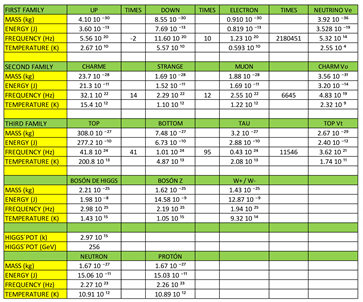
Table 32.
Energy, frequency and wavelength as a function of temperature.
Table 32.
Energy, frequency and wavelength as a function of temperature.
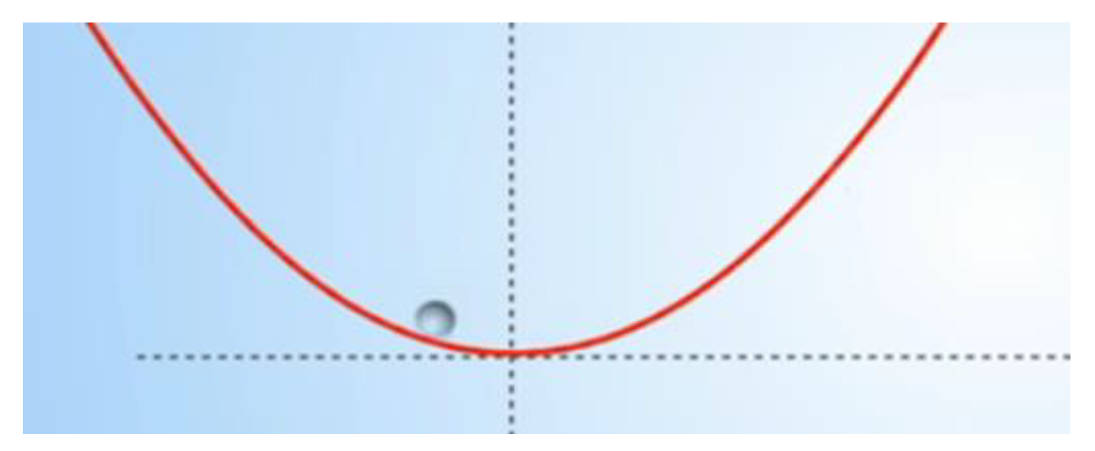
In my opinion, if we continue to lower the temperature, we will reach a critical point, an inflection point, in which a transition or phase change of matter will occur.
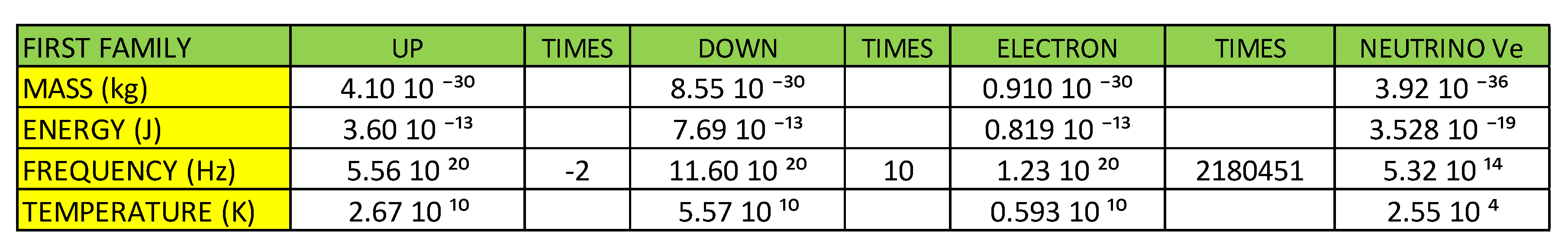
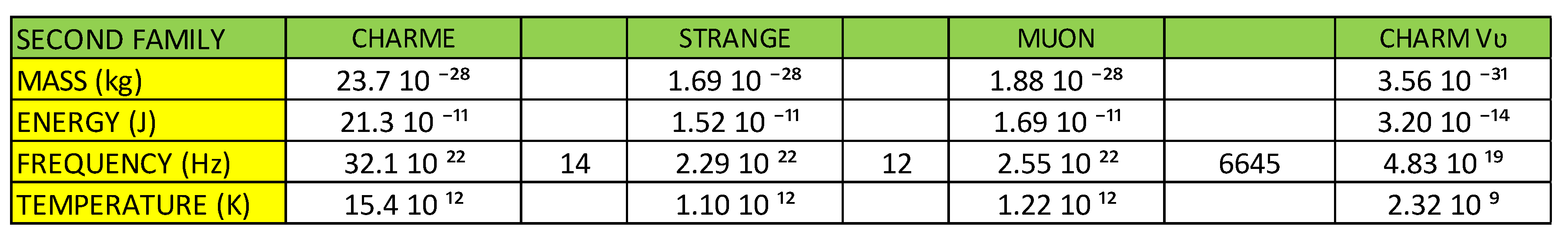
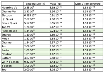
In item 7. ANALYSIS OF THE ORIGIN OF ELEMENTARY PARTICLES USING THE THEORY OF THE GENERALIZATION OF THE BOLTZMANN CONSTANT IN CURVED SPACE-TIME, we analyse how important temperature is in the formation of elemental particles.
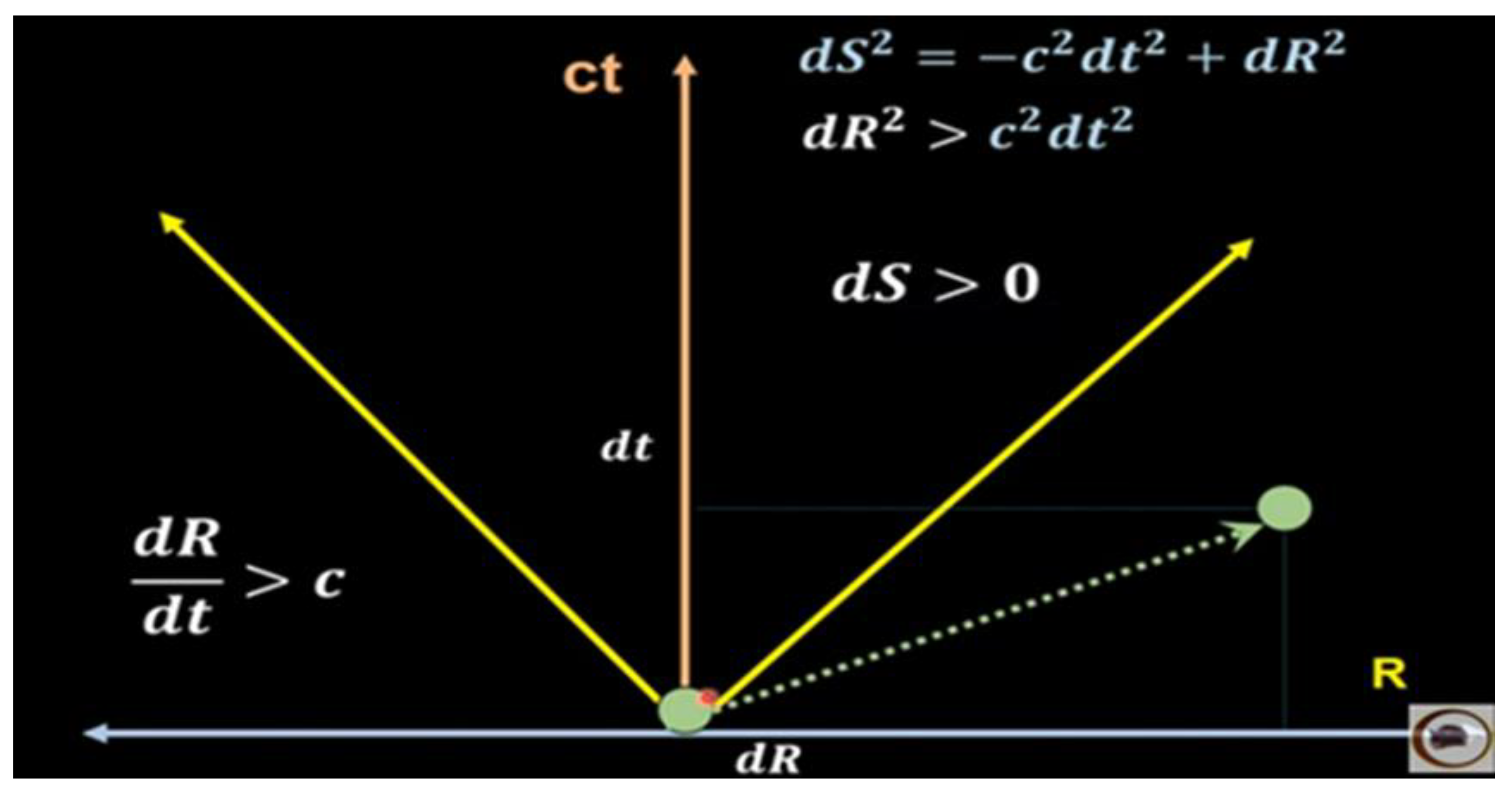
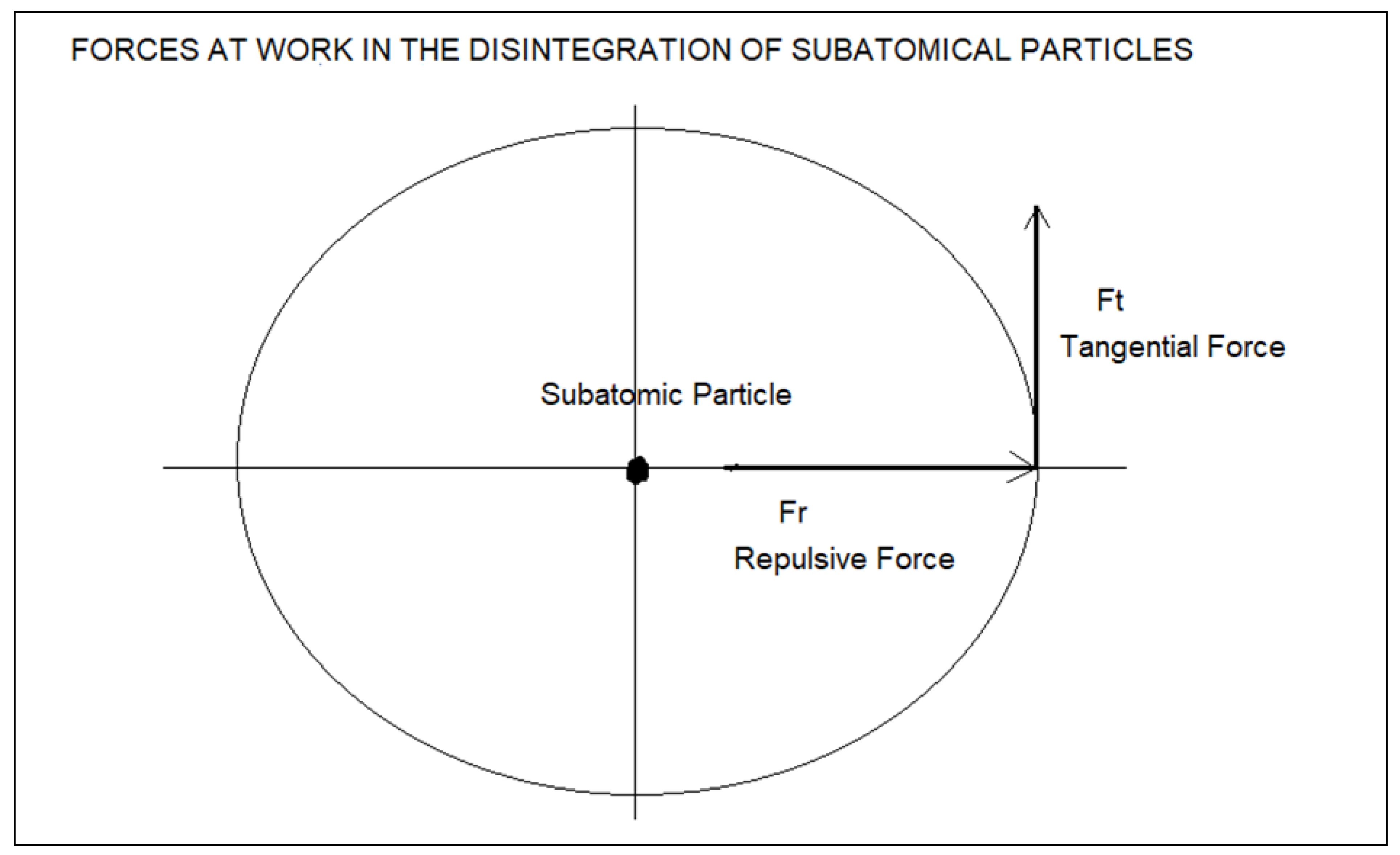
For low temperatures, the reverse process occurs, we will reach a critical inflection point Tc, in which the disintegration of the elementary particles occurs, separating the gravitons from the elemental electrical content.
The critical temperature, or inflection point, is the temperature at which the matter reaches (0) Kelvin.
This separation produces a repulsive force, which causes the temperature to reach values close to zero (0) kelvin.
In a simple analysis we are going to justify why the temperature reaches absolute zero, in an environment of repulsive gravity.
i) Let's consider the ideal gas equation:
PV = n Kв T
V = constant, repulsive forces act
ΔP V = n Kв ΔT
(Pf – Pi) V = n Kв (Tf – Ti)
In an environment in which repulsive gravity act, the final pressure will be lower than the initial pressure, therefore the value of (Pf - Pi) will be negative; this implies that the final temperature will be lower than the initial temperature.
In conclusion, in an environment in which repulsive gravity act, disintegration of matter, the temperature is zero (0) Kelvin.
The lower temperature limit corresponds to when the particles and bosons disappear. Only the elemental energy quanta remain in minimum energy values.
Example 6:
Quantum entanglement and the Bose-Einstein condensate
In the paper: RLC Electrical Modelling of Black Hole and Early Universe. Generalization of Boltzmann’s Constant in Curved Space-Time; we write the equation that defines the temperature of the Bose Einstein condensate:
According to the information of Cauê Muraro - Agência USP - 10/30/2007, the temperature of a Bose-Einstein condensate for 100,000 rubidium atoms corresponds to Tcmin = 180 nK.
Where Tcmin, low temperature Bose-Einstein condensate.
For Kв = 1.38 10⁻²³ J/K and rubidium atoms corresponds:
Tcmin = 180 nk
Approximate critical temperature of the Bose-Einstein condensate for low temperatures, with rubidium atoms.
Let's calculate Tcmax, for Kʙ-eff = 1.78 10⁻⁴³ J/K
Where Tcmax, High temperature Bose-Einstein condensate.
Tcmax, we are going to calculate considering the relationship between the Boltzmann´s constant Kʙ = 1.38 10⁻²³ J/K, for flat space-time and Kв-eff = 1.78 10⁻⁴³ J/K for curved space-time.
For Kʙ-eff = 1.78 10⁻⁴³ J/K and rubidium atoms corresponds:
Tcmax = 180 nk / 1.78 10⁻²⁰ = 1.01 10¹³ K
Tcmax = 1.01 10¹³ K
Critical temperature of the Bose-Einstein condensate for high temperatures with rubidium atoms.
Here we put forward the hypothesis that for an effective Boltzmann´s constant Kʙ-eff = 1.78 10⁻⁴³ J/K, there is a temperature Tcmax, that corresponds to a high temperature Bose Einstein condensate.
For a temperature of approximately 1.01 10¹³ K, in a plasma of quarks-gluons, a phase transition occurs that gives rise to a Bosonic condensate at high temperatures, which is characterized by being very energetic.
We can interpret it as follows, when a star collapses and a black hole is formed, we can affirm that a high-temperature Bose-Einstein condensate exists inside a black hole.
In analogy with the properties of materials at very low temperatures, super fluids and superconductivity; quark-gluon plasma achieves similar exotic properties, but not with atoms and molecules as we normally know.
these properties are achieved for the quark-gluon plasma, a superfluid or super solid, the main property of which makes this liquid or solid behave like isolated quarks, allowing the gluons to stack up neatly in an infinite cascade of energy; making it the most energetic matter in the universe.
We also said that quarks are fermions and gluons are bosons, but in black holes, by analogy with what happens with superconducting materials and super fluids and super solids; the plasma of quarks and gluons as a whole act as a Bose-Einstein condensate, as a single atom whose macroscopic properties are unique.
Here we hypothesize that quantum entanglement is related to the Bose-Einstein condensate, that is, there is quantum entanglement for a Bose-Einstein condensate of low temperature Tcmin and there is also quantum entanglement for a Bose-Einstein condensate of high temperature Tcmax.
We are familiar with low temperature quantum entanglement, Tcmin, in quantum computers, for Kʙ = 1.38 10⁻²³ J/K.
At high temperatures, Tcmax, for Kʙ = 1.78 10⁻⁴³ J/K, quantum entanglement is given to calculate the viscosity of the quark-gluon plasma.
Using duality DST (ADS) = EFQT (CFT)
We can use the Boltzmann´s constant of the quark-gluon plasma or eventually the Boltzmann´s constant for a black hole, interchangeably, to calculate the viscosity of the quark-gluon plasma, which will give us the same result.
Boltzmann´s constant for quark-gluon plasma: Kʙ-eff = 0.76 10⁻⁴¹ J/K.
Boltzmann´s constant for black hole: Kʙ-eff = 1.78 10⁻⁴³ J/K.


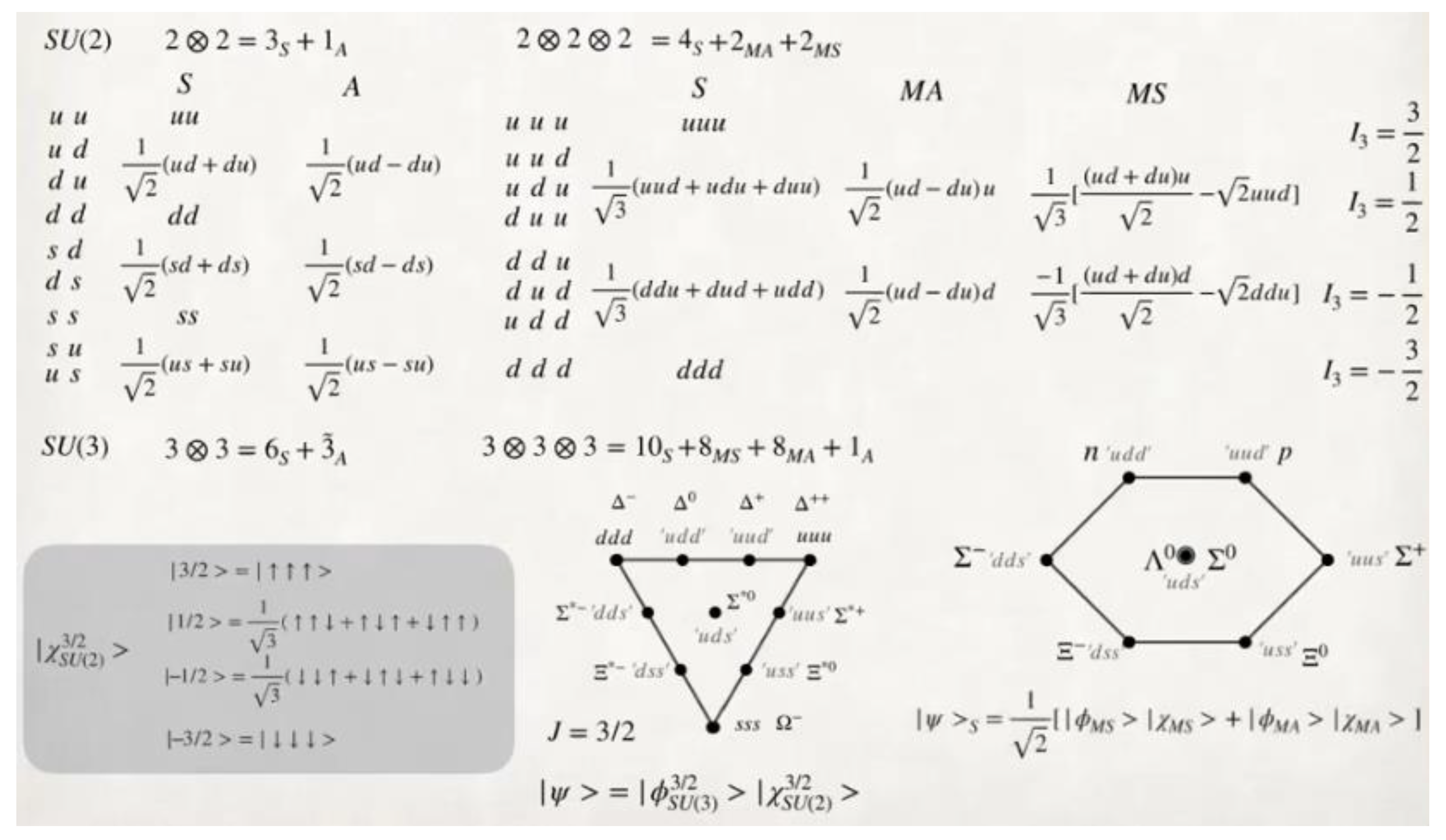
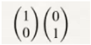 , fundamental, representation.
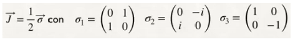
 , fundamental,
representation.
, fundamental,
representation.
 Where λa are Gell-Mann, matrices.
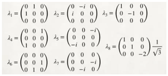
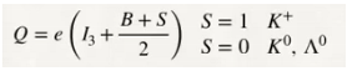
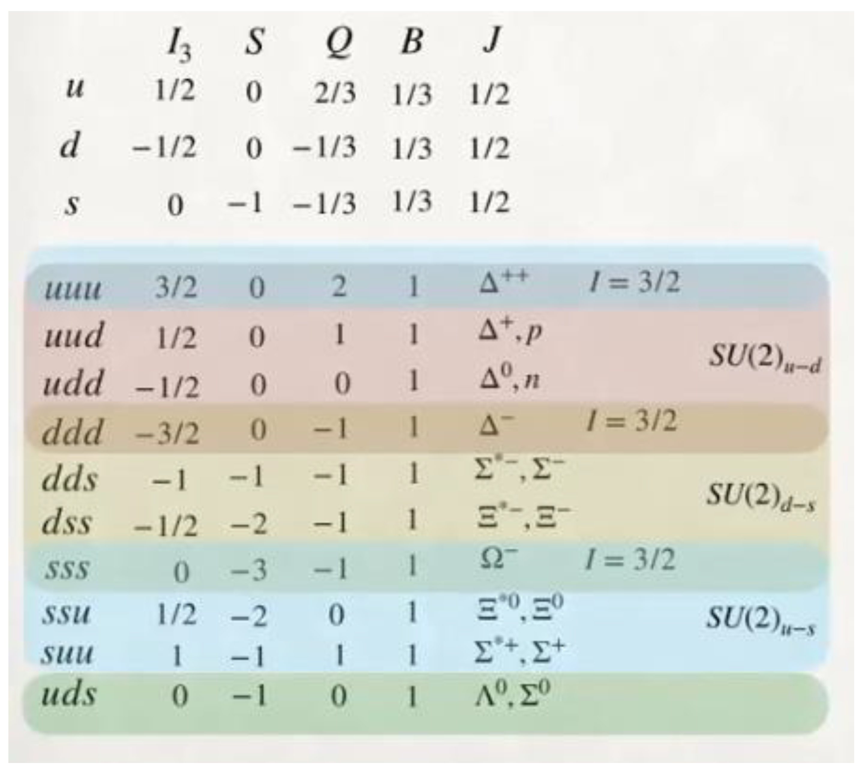
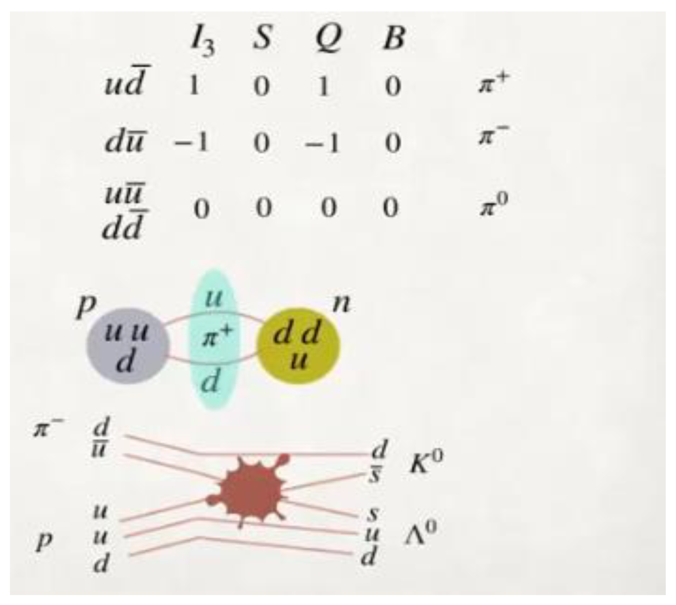
 B = 1, baryons; B = 0,
mesons.
B = 1, baryons; B = 0,
mesons.