
Submitted:
08 January 2024
Posted:
09 January 2024
You are already at the latest version
Abstract
Passive marine listening, involving the acoustic monitoring of underwater environments, has become increasingly vital for scientific research, environmental monitoring, and defense applications. However, the success of such applications critically depends on the ability to extract meaningful information from the often noisy and dynamic underwater acoustic environment. In this context, Mel-frequency cepstral coefficients (MFCCs) have emerged as an essential tool for feature extraction, capturing the spectral characteristics of marine sounds and making them ideal for species identification and sound event detection. This research presents an innovative approach to enhance the robustness of MFCC-based passive marine listening through adaptive noise reduction techniques. The proposed approach utilizes dynamic spectral subtraction to counter underwater noise, resulting in enhanced signal-to-noise ratios for desired sounds. This adaptive system adjusts to dynamic underwater noise, allowing it to concentrate on target sounds and suppress interference effectively. The experimentation further validates the effectiveness of the proposed approach, with results reaching 99% on the full dataset of 570 mammals and vessels, demonstrating the effectiveness of SVM and Random Forests in the classification of underwater audio.
Keywords:
MFCC
; spectral subtraction
; svm
; random forests
; feature engineering
1. Introduction
The underwater soundscape is a rich repository of information, housing the vocalizations of marine species, underwater geological phenomena, and the presence of vessels. Mel-frequency cepstral coefficients (MFCCs) represent a fundamental tool in the realm of audio signal processing, establishing themselves as foundational instruments for the analysis of audio signals. MFCCs are used in diverse applications, from speech and speaker recognition to music analysis and acoustic signal processing. They achieve this by first transforming the audio signal into a Mel-frequency scale to mirror human perception, then dividing it into frames to extract spectral information. This process yields a compact representation of the most salient features, making MFCCs invaluable for tasks like sound classification, environmental monitoring, and species identification, while also proving their worth in the broader landscape of digital signal processing. In the complex and dynamic underwater acoustic environment, the application of Mel-frequency cepstral coefficients (MFCCs) encounters notable limitations. Strong underwater noise, emanating from natural sources such as waves and wind, as well as anthropogenic activities like ship traffic, poses a formidable challenge to the accuracy of MFCC-based analyses. The robustness of MFCCs diminishes in the presence of noise, as they often struggle to differentiate between the desired signals, such as marine species vocalizations, and the pervasive noise. Variations in the noise characteristics due to factors like water conditions, weather, and marine life activity further compound the limitations of MFCCs in underwater settings. As a result, to maximize the utility of MFCCs in this demanding soundscape, the integration of adaptive noise modeling and other advanced noise reduction techniques is essential, emphasizing the need for a comprehensive approach in underwater acoustic analysis. Adaptive noise reduction techniques are a pivotal component of audio signal processing, designed to alleviate the impact of unwanted noise in various applications. These methods are especially valuable in scenarios where the noise environment is dynamic and unpredictable. They adapt to the changing noise conditions by estimating noise characteristics and actively reducing its presence in the signal, enhancing the clarity of the desired sounds. When incorporated into the MFCC feature extraction process, these adaptive filters offer significant advantages. By reducing noise interference before feature extraction, they provide cleaner and more accurate representations of the acoustic signals. This, in turn, enhances the efficacy of MFCCs in capturing the critical spectral characteristics of audio data, making them more resilient in the presence of noise. The integration of adaptive noise reduction techniques into MFCC feature extraction has garnered attention as a powerful approach to address the inherent challenges of underwater noise, it proves particularly advantageous in tasks such as speech recognition, environmental monitoring, and marine species identification, where noise robustness is paramount for accurate and reliable analysis.
2. Background
MFCCs are like building blocks for processing sound. They help us understand the different aspects of how sounds are made.Derived from models of human auditory perception, MFCCs assume a pivotal role across a spectrum of applications, establishing themselves as an indispensable element within the toolkit for acoustic signal analysis. In the domain of voice recognition, MFCCs have played a foundational role. Leveraging the human auditory system’s sensitivity to different frequency bands, MFCCs capture the distinctive spectral characteristics of speech signals. The paper [1] introduces a novel approach to enhance Mel-frequency cepstral coefficients (MFCCs) for speech and speaker recognition by replacing the logarithmic transformation with a combined function and integrating speech enhancement methods, resulting in a robust feature extraction process that significantly reduces recognition error rates across diverse signal-to-noise ratios. An innovative MFCC extraction algorithm [2] for speech recognition that significantly reduces computation power by 53% compared to conventional methods, with a minimal 1.5% reduction in recognition accuracy, making it highly efficient for hardware implementation due to a halving of required logic gates. MFCCs have been extensively employed in emotion recognition from speech. Studies like ’Emotion Detection Using MFCC and Cepstrum Features’ [3] focuses on Speech Emotion Recognition (SER), evaluating the impact of cepstral coefficients and conducting a comparative analysis of cepstrum, Mel-frequency Cepstral Coefficients (MFCC), and synthetically enlarged MFCC coefficients, demonstrating improved recognition rates for seven emotions compared to prior work, particularly surpassing an algorithm by InmaMohino in reducing misclassification efficiency. Research in [4] explores emotion recognition from speech using a 3-stage Support Vector Machine classifier, leveraging MFCC features and statistical measurements from the Berlin Emotional Database, achieving a 68% accuracy through hierarchical SVM with linear and RBF kernels and 10-fold cross-validation. MFCCs have found applications beyond human-centric contexts, extending to environmental monitoring and species identification. For instance, in ’Automatic recognition of animal vocalizations using averaged MFCC and linear discriminant analysis’ [5] a method utilizing averaged Mel-frequency cepstral coefficients (MFCCs) and linear discriminant analysis (LDA) is proposed to automatically identify animals from their sounds, achieving high classification accuracies of 96.8% for 30 kinds of frog calls and 98.1% for 19 kinds of cricket calls. The study in [6] proposes a drone recognition method using Mel frequency cepstral coefficients (MFCCs) for feature extraction and hidden Markov models (HMMs) for classification based on drone propeller sounds, achieving high recognition rates even in noisy environments. ’Acoustic Classification of Singing Insects Based on MFCC/LFCC Fusion’ [7] introduces a novel approach for automatic identification of crickets, katydids, and cicadas through acoustic signals, achieving an outstanding 98.07% success rate at the species level using Mel Frequency Cepstral Coefficients (MFCC) and Linear Frequency Cepstral Coefficients (LFCC), particularly showcasing the efficacy of their fusion. The article [8] proposes a heart sound classification method using improved Mel-frequency cepstrum coefficient (MFCC) features and convolutional recurrent neural networks, achieving a remarkable 98% accuracy for the two-class classification problem (pathological or non-pathological) on the 2016 PhysioNet/CinC Challenge database. As demonstrated by these applications, MFCCs offer a versatile framework for extracting meaningful features from audio signals, transcending their initial role in voice analysis. The adaptability and effectiveness of MFCCs make them a cornerstone in various fields, continually contributing to advancements in audio signal processing and pattern recognition.
3. MFCC Robustness Approach
This section offers an elaborate exposition of our proposed algorithm, encapsulating three fundamental components: MFCC feature extraction, adaptive noise reduction, and classification models. Figure 1 illustrates the overall flowchart of the proposed method. Prior to feature extraction, the raw audio data undergoes several processing steps, including amplitude normalization, resampling, and removal of unnecessary components. Adaptive noise reduction technique is used to adjusts to changing environmental conditions. It greatly improves the accuracy of target signal identification in difficult underwater environments by ensuring robust noise suppression and enhancing the precision of MFCC-based feature vectors. The subsequent stages involve smooth frame segmentation, windowing using the Hamming function to mitigate spectral leakage, and computing the Short-Time Fourier Transform (STFT) for each frame. Afterwards, the training database is constructed by applying the discrete cosine transform (DCT), logarithmic compression, and Mel filterbanks. Following this, the labeled features are fed into the classification models for training and identification.
3.1. Noise Reduction
Noise introduces a potential source of degradation for Mel-Frequency Cepstral Coefficients (MFCCs) in underwater applications. The complex underwater acoustic environment, which is frequently characterized by high background noise, makes it difficult to accurately extract pertinent acoustic information. It is critical to acknowledge the need for effective noise reduction strategies, particularly in situations when sounds from mammals or vessels mix with significant background noise. To improve the reliability of MFCC, it is imperative to apply efficient noise reduction techniques. However systems such as the Raspberry Pi 4 have processing limitations that necessitate careful algorithm selection. In this context, spectral subtraction emerges as a computationally feasible and effective method for noise reduction, offering a balance between performance and computational cost suitable for real-time processing on resource-constrained devices. The noisy signal model in the frequency domain is given by equation 1 where Y, , and are the signal, the additive noise, and the noisy signal respectively.
3.1.1. Noise Estimation
During our work in [9] we meticulously prepared a set of reference noise profiles. This comprehensive collection encapsulates diverse environmental conditions encountered over a week-long period. The considered scenarios span a spectrum of atmospheric and oceanic states, including calm conditions, wind and wave variation, rainfall, stormy weather, clear skies, and day and night. When estimating the noise spectrum, one often uses the time-averaged noise spectrum from the portions of the recording that include just noise. The noise estimate is given by:
where the amplitude spectrum of the of the K noise frames is denoted by . A first-order low-pass filter can be used to filter the noise and generate a noise estimate in the frame.
where is the smoothed noise estimate in i-th frame and is the low pass filter coefficient. The phase of the noisy signal and the magnitude spectrum estimate are combined to restore a time domain signal. The time is then converted into the discrete Fourier transform via the inverse method, as follows:
where is the phase of the noisy signal frequency Y(k).
3.1.2. Spectral Subtraction
The magnitude spectrum subtraction is defined as:
where is the time-averaged magnitude spectrum of the noise. For signal restoration the magnitude estimate is combined with the phase of the noisy signal and then transformed into the time. Taking the expectation of equation 5 we have:
3.1.3. Continuous Noise Monitoring
An integration between time-varying noise models and environmental sensors is presented to improve the adaptability of the noise reduction process in underwater environments. Contextual information is further enhanced by environmental sensors, which may monitor things like weather patterns, marine activities, and water quality. With the use of this data, the noise reduction system’s parameters are dynamically changed to better accommodate shifting acoustic conditions. The environmental sensor data at time t is represented by C(t), and the time-varying noise standard deviation is indicated by . The following is the modified version of the time-varying noise model:
where represents the standard deviation of the environmental sensor data at time t, and is a smoothing factor. Contributing to the resilience of the noise reduction system, this adaptive technique makes sure that the noise model takes into account variations in the undersea environment.
3.2. MFCC Calculation
The feature extraction outlines a methodical approach to using Mel-frequency cepstral coefficients (MFCCs) for noise reduction in audio processing. The manual covers the following topics: Data Collection, Frame Segmentation, Windowing, Short-Time Fourier Transform (STFT), Mel-Frequency Filterbanks, Discrete Cosine Transform (DCT), and Feature Vector Extraction.
3.2.1. Data Collection
In our project, we have curated a comprehensive training dataset comprising a total of 558 audio samples sourced from two distinct databases. The primary source is the Watkins Marine Mammal Sound Database / New Bedford Whaling Museum [10], contributing 480 samples representing a diverse array of 32 marine mammal species. This dataset encompasses a broad spectrum of vocalizations, allowing for a robust training foundation to capture the acoustic nuances of various marine species. Additionally, we have incorporated 78 samples of ships’ noise from the ShipsEar database [11], specifically chosen to simulate real-world scenarios involving underwater vessel noise. This inclusion addresses the need to develop a model that can effectively discriminate between marine mammal sounds and the potential interference posed by ship noise. Table 1 illustrates the proposed data split, with 60% of each class for both mammal and vessel sound allocated to the training set, 20% for the validation set, and 20% for the testing set.
3.2.2. Segmentation
The initial step involves dividing the continuous audio signal into distinct frames . In the pursuit of segmentation, the procedure outlined in [12] involves the identification of adjacent signal peaks until a predefined threshold is attained. Following the detection of a discernible pattern, the recording is meticulously sliced to extract individual samples, each of which is then systematically stored in the database. This process employs a rectangular window function , ensuring frame continuity. The frame length () and overlap () parameters govern the segmentation process.
3.2.3. Windowing
After segmentation, a Hamming window is applied to each extracted frame for refining. For signal framing, the Hamming window function is used because it may effectively mitigate the leakage phenomena. To provide a seamless transition between frames, 40% overlaps are used between successive frames. The Hamming window function for is defined as:
where N is the length of the window, provides the tapering effect smoothly transitioning from 1 to -1 as n goes from 0 to N - 1, factor 0.54 is used to normalize the amplitude of the window, and 0.46 is the correction factor to minimize the first sidelobe of the window. By element-wise multiplication, each segmented frame is then modulated by the Hamming window, resulting in frames endowed with improved spectral characteristics.
3.2.4. Short-Time Fourier Transform (STFT)
The Short-Time Fourier Transform (STFT) serves as a powerful tool for revealing the frequency content of a signal over short overlapping time intervals, it involves taking the Fast Fourier Transform (FFT) of the windowed frame to obtain the magnitude and phase spectra.The STFT is defined as follows:
where represents the Fourier transform of the frame of the signal , obtained by applying a Hamming window . The STFT enables the representation of signal components in both time and frequency domains simultaneously, providing insights into the spectral characteristics of the signal over distinct temporal segments.
3.2.5. Mel-Frequency Filterbanks
After the Short-Time Fourier Transform (STFT) provides a time-frequency representation, MFCCs utilize Mel-Frequency Filterbanks defined by the equation:
The function represents the contribution of the filter to the frequency bin. Equation 11 defines a set of triangular-shaped functions (Mel-Frequency Filterbanks) used to model the non-linear frequency perception of the human ear. The filterbanks emphasize frequencies in a way that is consistent with human auditory perception, with higher resolution at lower frequencies. The Mel scale to the response frequency is computed by equation 12
3.2.6. Discrete Cosine Transform (DCT)
Following the derivation of MFCCs, the DCT is applied to the logarithmically compressed filterbank energies, aiming to decorrelate these coefficients and extract the most salient features. The Mel filterbanks capture the perceptually significant frequency bands, and subsequently, the MFCC () is computed using the equation:
where represents the Mel filterbank energies derived from the STFT magnitude spectrum. The power exponent p in equation 13 serves to amplify the significance of dominant spectral components and further improves the discriminative power of MFCCs, making them more resilient to variations and noise in the audio signal.
3.2.7. Feature Vector Extraction
Feature Vector Extraction involves distilling essential information from the Discrete Cosine Transform (DCT)-decorrelated coefficients obtained, particularly in the computation of Mel-Frequency Cepstral Coefficients (MFCCs). Following the DCT application to the logarithmically compressed Mel filterbank energies, the feature vector is derived by selecting a subset of coefficients. Mathematically, this can be represented as: Feature Vector = where denotes the DCT coefficient chosen for the feature vector.
3.3. Classification Model
Our study focuses on the pragmatic use of Support Vector Machines and Random Forests for audio classification [13]. While Convolutional Neural Networks (CNNs) have demonstrated remarkable performance where input data exhibits spatial relationships as seen in image data, the constraints of the Raspberry Pi 4 lead us to consider simpler models. The decision to opt for these models is rooted in the unique characteristics and size of our dataset, in addition to the computational limitations on a resource-constrained device.
3.3.1. SVM Classifier
The core principle of SVM involves finding the hyperplane that best separates different classes in the feature space while maximizing the margin between them. In this context of underwater audio, where diverse marine sounds may exhibit complex patterns that require a flexible and expressive classifier, SVMs are particularly advantageous due to their ability to handle high-dimensional feature spaces, making them well-suited for the intricate acoustic characteristics captured by MFCCs. Considering the problem of approximating the dataset D consisting of N samples:
where each sample consists of a feature vector in and a corresponding label in R. Mathematically, the decision function of a kernelized Support Vector Machine (SVM) is represented as:
where represents the weight vector, is the feature mapping of input , and b is the bias term. The kernel trick facilitates the computation of dot products in a higher-dimensional space, eliminating the need for explicit calculation of the feature mapping .
With K denoting the inner product between the mapped features of two input samples. The optimization problem for the kernelized SVM involves minimizing a quadratic objective function subject to constraints
With as the Lagrange multipliers, the class label, and K is the kernel function. The decision function used for making predictions in a kernelized SVM is illustrated in:
Equation 18 represents a weighted summation of the kernel evaluations between the input and the support vectors. The objective function for solving the quadratic programming problem associated with the SVM is represented in:
With Q denoting the margin between classes within the feature space. The kernelized Support Vector Machine (SVM) employs a kernel function K to implicitly project the input data into a higher-dimensional space, facilitating the classification of non-linearly separable datasets. The optimization problem is framed using the kernelized decision function, and the task involves determining the optimal set of Lagrange multipliers that maximizes the margin while adhering to the specified constraints. Additionally, the prediction function for new data points is kernelized, empowering the SVM to operate proficiently in feature spaces beyond the original input space.
3.3.2. Random Forest Classifier
The Random Forest Classifier is an ensemble learning method that operates by constructing a multitude of decision trees at training time and outputs the mode of the classes of the individual trees for classification tasks. Each decision tree in the forest is trained on a random subset of the training data and uses a random subset of features at each split point, introducing variability and decorrelation among the trees. The final prediction is then made by aggregating the predictions of all individual trees.
where f(x) is the prediction for input x, N is the number of leaf nodes in the decision tree, is the class assigned to the leaf node, is the region associated with the leaf node, is an indicator function that outputs 1 if x belongs to and 0 otherwise. The Random Forest prediction equation 21 combines the predictions of individual decision trees in the forest to make a final prediction. Given a new input x the Random Forest prediction is the average of the predictions from all the individual trees.
where is the final prediction of the Random Forest, M is the number of trees in the forest, is the prediction of the decision tree.
4. Experiment
To assess the efficacy of the proposed work, a comprehensive evaluation was conducted across three distinct testing scenarios. The first experiment tests the identification sensitiveness between mammals and vessels. The second focuses on the identification and classification of mammal species, followed by the third scenario, involving the identification and classification of different vessel types.
4.1. Data Acquisition
The algorythm is devised to capture acoustic data from 2 separate microphones upon the detection of sound exceeding a predetermined threshold. The monitoring of audio inputs is accomplished through the implementation of a dynamic threshold-checking function, wherein the amplitude of audio frames is evaluated for a defined number of consecutive frames set. This approach ensures ensures audio recording exclusively when the acoustic environment surpasses the established threshold for an extended period, affording a reliable mechanism for capturing meaningful auditory events. The resulting audio recordings are meticulously organized into date-based folders and uniquely labeled with device indices and timestamps. By integrating variable ambient noise, the script facilitates the generation of audio that closely mimic the diverse environmental conditions found in real-world scenarios. Following the loading the original ambient noise, random values within a predefined range are generated to act as scaling factors. These random values are then used to mix the ambient noise with the original recording, resulting in each recording having a unique level of added noise. The recording parameters employed in the audio capture system are tailored to ensure efficient and accurate data acquisition. The chunk size is set to 1024, specifying the number of samples to be recorded in each iteration. A recording precision of 16 bits per sample allows for more detailed representation of the audio signal, enhancing the fidelity of the recorded data. A mono recording configuration is chosen to simplify data processing and storage. A sampling rate of 48000 represents the rate at which the analog audio signal is converted into a digital representation.
4.2. Setup
The setup utilizes a Raspberry Pi 4 (see Figure 2a), two SN005 hydrophones (see Figure 2b), and an LT-015 underwater speaker (see Figure 2c) in a 4.5x2.2x0.84 meter swimming pool (see Figure 2d).The controlled environment provides insights into underwater sound dynamics in a confined space, offering valuable data for applications in aquatic event monitoring, marine life studies, and underwater communication research. A 12000mAh power bank powers the Raspberry Pi 4 within the floating buoy. The power bank is selected for its portability and sufficient capacity for the experiment’s duration.
Raspberry Pi 4 (4GB)
- The central processing unit responsible for signal acquisition, processing, and data storage. Housed within a floating buoy for mobility.
- The integrated Ethernet, Wi-Fi, and Bluetooth capabilities make it simple to connect to other devices and networks, and its GPIO pins facilitate easy integration with hardware components like sensors.
- Features a powerful quad-core 64-bit ARM Cortex-A72 CPU with 4GB of RAM, providing ample processing power for MFCC calculation
Hydrophones (SN005)
- 150g omnidirectional hydrophones positioned at the pool’s base in a linear array configuration and are directly connected to the USB ports of the Raspberry Pi 4 for real-time data acquisition.
- With a wide frequency range of 40 to 14000Hz and an exceptionally high sensitivity of approximately -28dB, it is suitable for various applications, including underwater recordings.
- Can operate in temperatures between -40°C and 60° with an IP68 waterproof rating, operates at a low working current of approximately and interfaces with devices within a working voltage range of 1.5V to 5V.
Underwater Speaker (LT-015)
- A 40W underwater speaker mounted on the 2.2-meter side, submerged 20cm underwater to ensure a 180-degree delivery angle within the pool.
- With a rated power of 60W and a maximum power capability of 90W, this speaker delivers a robust performance even in challenging underwater environments.
- Features a running impedance is 80 ohms and covers a substantial frequency range from 80 to 18,000Hz
Swimming Pool
- Dimensions: 4.5x2.2x0.84 meters.
- Controlled environment for studying underwater sound propagation. The pool provides a confined space for acoustic signal analysis.
- The 0.84 meters depth provides an opportunity to study sound propagation under different water depths, contributing to a comprehensive analysis of acoustic behavior.
4.3. Feature engineering
Feature engineering assumes a crucial role in the extraction of meaningful patterns from audio data, utilizing the waveform of sound files as the primary source of information. This process involves transforming raw audio signals into a format suitable to model training, extracting relevant information, reducing dimensionality, and enhancing the model’s ability to discern patterns. Spectrogram representation converts audio signals into time-frequency representations, capturing essential characteristics such as pitch and intensity. Mel-Frequency Cepstral Coefficients (MFCCs) provide insights into spectral characteristics and are particularly useful in speech and audio processing. Chroma features highlight pitch content, aiding in tasks like musical genre classification. Other features like Rhythm patterns and Spectral contrast are also studied. These techniques not only reduce dimensionality and accelerate model training but also enable models to discern intricate patterns, making feature engineering the linchpin for success in audio-related machine learning tasks.
4.3.1. Mel-Frequency Cepstral Coefficients (MFCCs)
Mel-Frequency Cepstral Coefficients process involves transforming the frequency-domain information of the audio signal into a set of coefficients that represent the short-term power spectrum of the sound. The steps in extracting MFCC involve framing the signal, applying a Fourier Transform, mapping the spectrum to the mel scale, taking the logarithm of the powers, and finally applying a Discrete Cosine Transform (DCT) to obtain the coefficients.
The bowhead whale’s figure exhibits broader distribution of frequency components capturing the deep, resonant nature of its calls. On the other hand, the fishing vessel engine graph is characterized by a concentration in the higher frequencies. By visually inspecting and comparing these MFCC spectra, we can gain valuable insights laying the foundation for further analysis and classification for the unique acoustic fingerprints of marine acoustic.
4.3.2. Mel Spectrogram
The Mel spectrogram is a type of spectrogram that utilizes the Mel scale, a perceptually relevant frequency scale, to represent the distribution of energy in an audio signal over time. It is obtained by applying a Mel filterbank to the Short-Time Fourier Transform (STFT) of the signal.
Figure 4.
Mel Spectrogram.
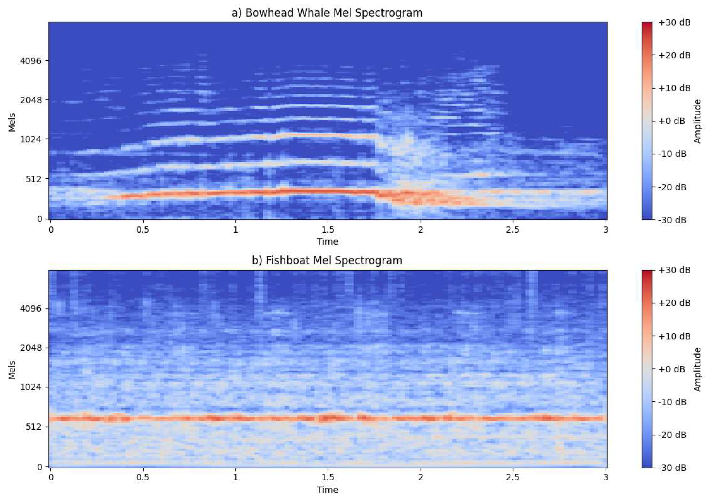
The Bowhead Whale’s spectrogram reveals intricate patterns characterized by clear transitions between multiple Mel frequency peaks. These transitions are indicative of the whale’s communication repertoire. In contrast, the fish boat’s spectrogram exhibits a singular, robust peak, distinctly representing the mechanical hum of its propulsion system.
4.3.3. Power Spectrogram
A power spectrogram is a visual representation of the distribution of power across different frequencies in a signal over time. It is obtained by taking the squared magnitude of the Short-Time Fourier Transform (STFT) of a signal.
Figure 5.
Power Spectrogram.
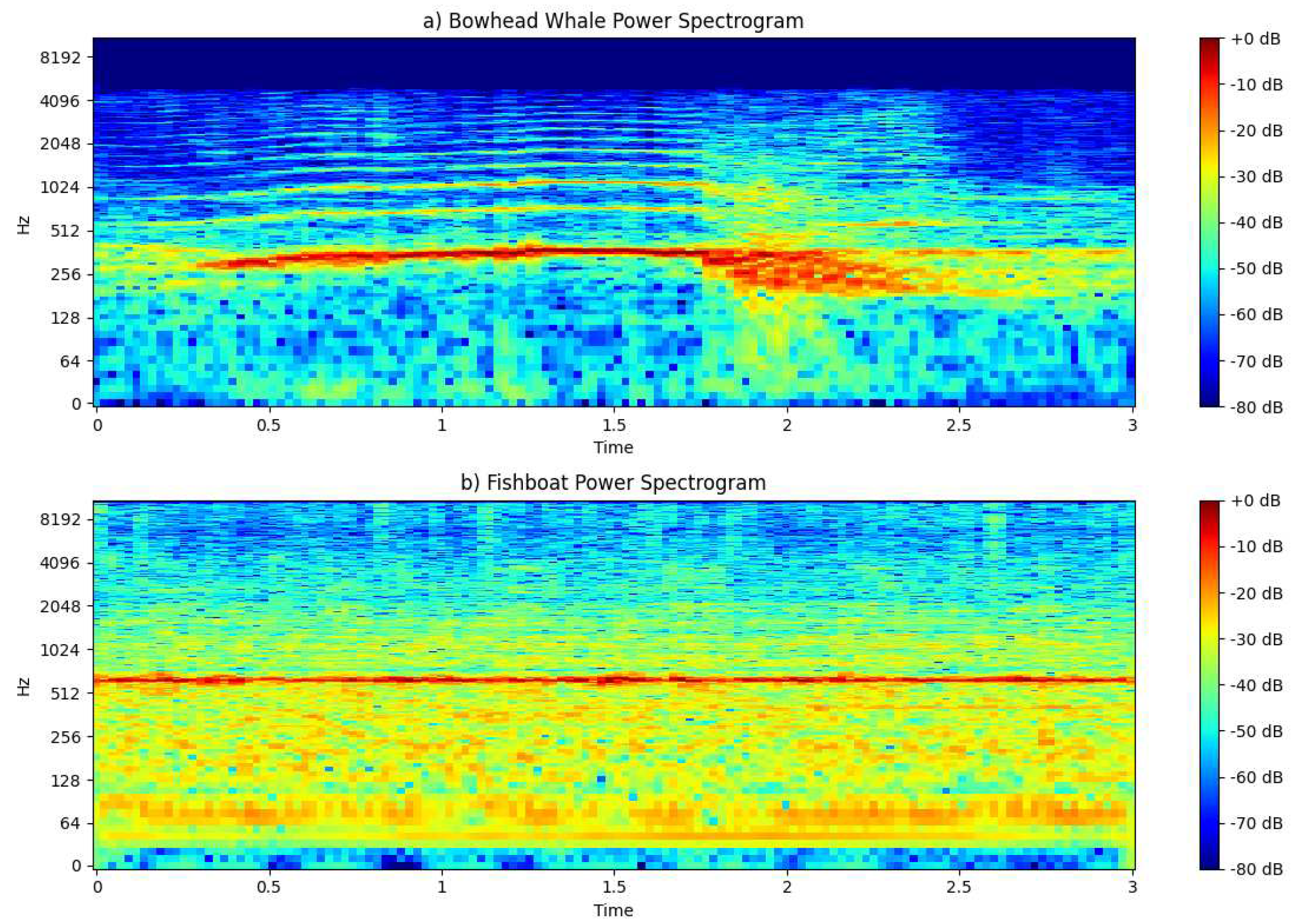
The analysis of the power spectrogram further enriches our understanding of the acoustic characteristics of the bowhead whale and the fish boat. Notably, the power spectrogram of the bowhead whale exhibits a pronounced and consistently higher magnitude of power at each time-frequency point compared to the vessel.
4.3.4. Chromagram
A chromagram is a representation of the distribution of pitch classes in an audio signal. It provides a condensed view of the tonal content, disregarding the octave of each note. The chromagram is derived by mapping the energy distribution of the signal onto the 12 different pitch classes, representing the notes in the chromatic scale.
Figure 6.
Chromagram.
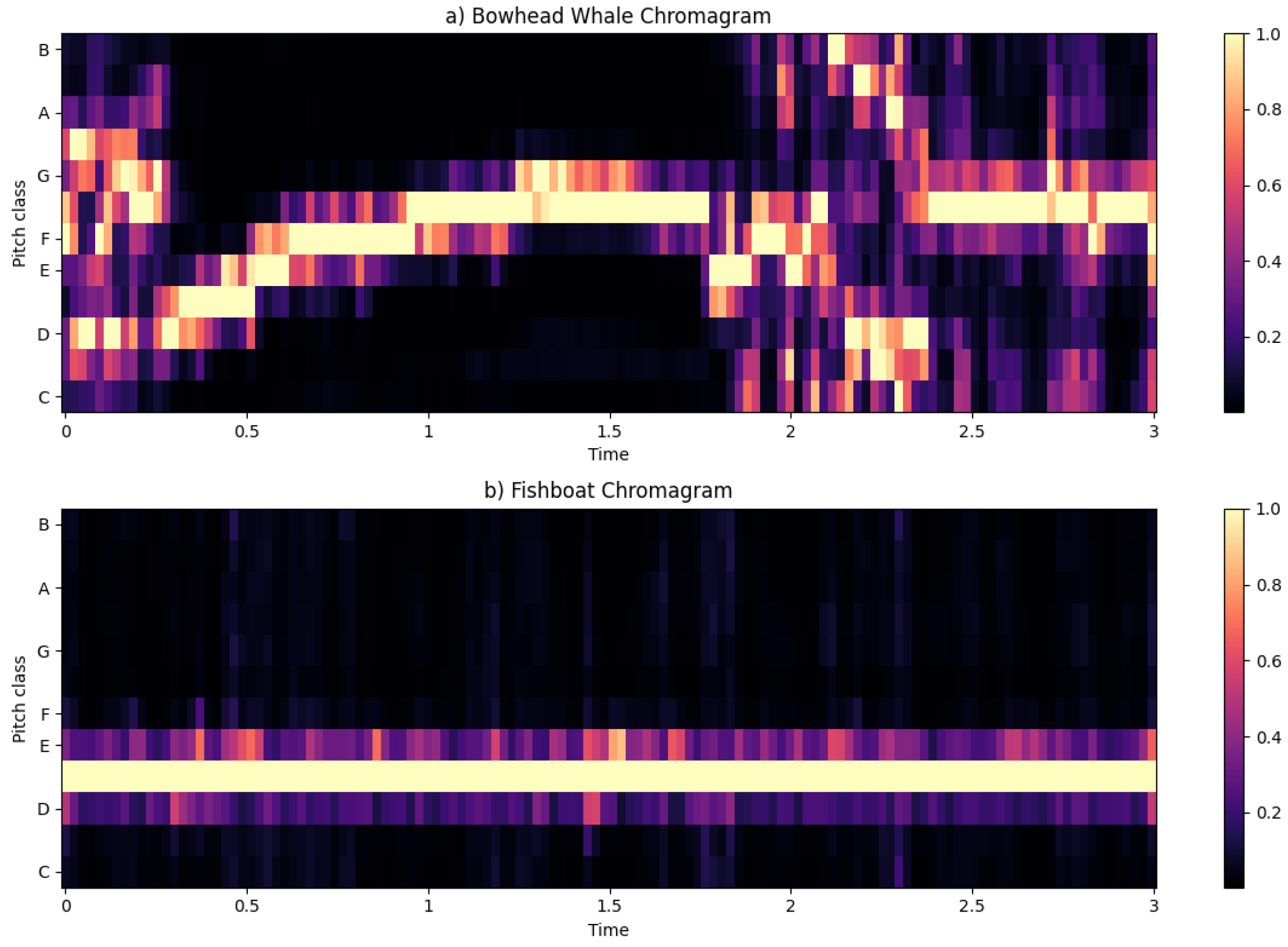
The fish boat’s pitch distribution exhibits a notable dispersion solely in the lower region, indicating a concentrated presence of lower-frequency components. In contrast, the bowhead whale’s pitch distribution varies dynamically from low to high regions over time, with a discernible concentration in the medium region.
4.3.5. Other Features
In addition to feature extraction methods such as Mel-Frequency Cepstral Coefficients (MFCC), Chroma, and power spectrograms, our exploration extends to encompassing features like rhythm patterns and spectral contrast. Rhythm patterns encapsulate the temporal aspects of an audio signal, capturing nuances in timing and rhythmic structures. On the other hand, spectral contrast emphasizes the differences in energy distribution between peaks and valleys in the frequency spectrum, providing insights into tonal variations.
Figure 7.
Rhythm Patterns.
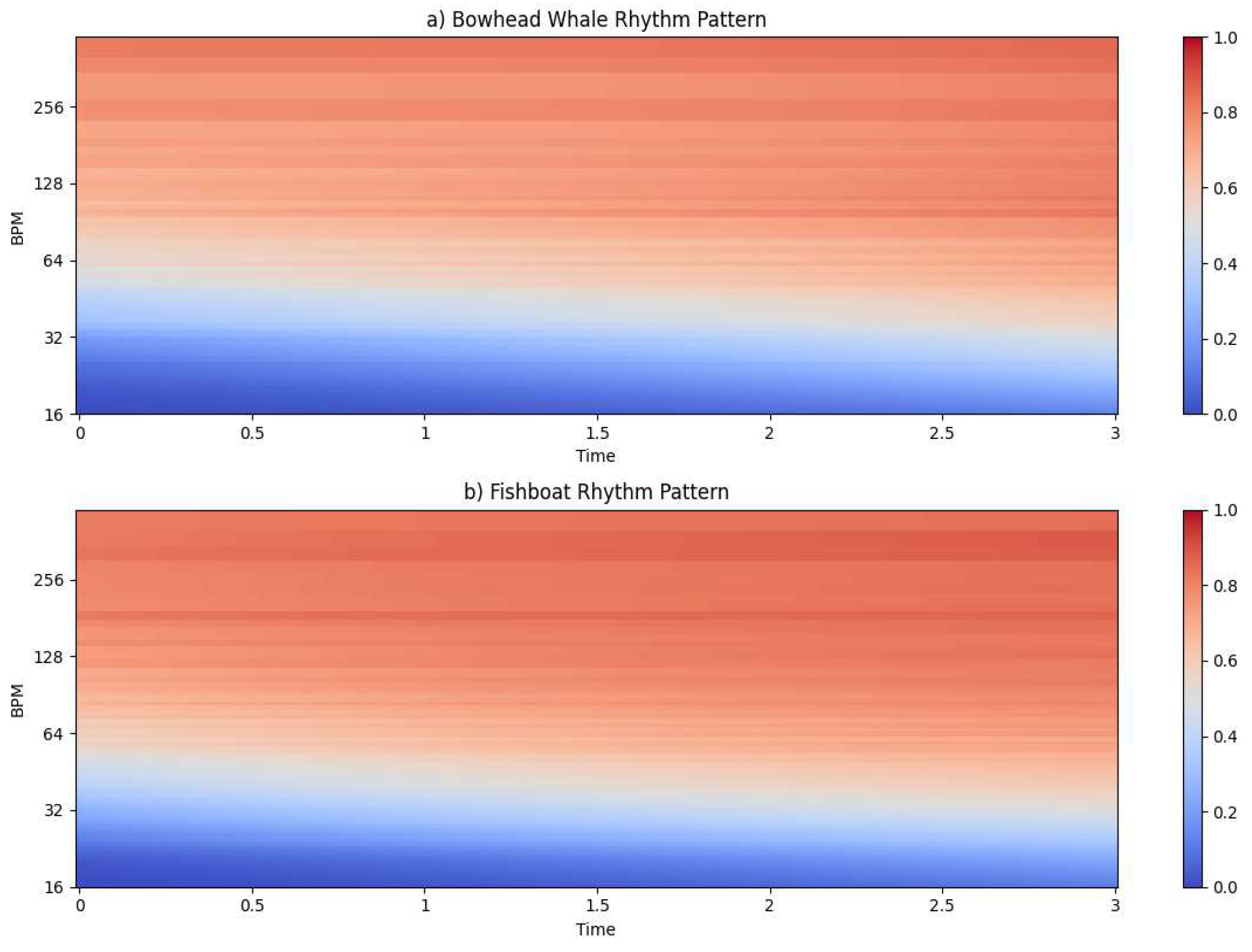
Figure 8.
Spectral Contrast.
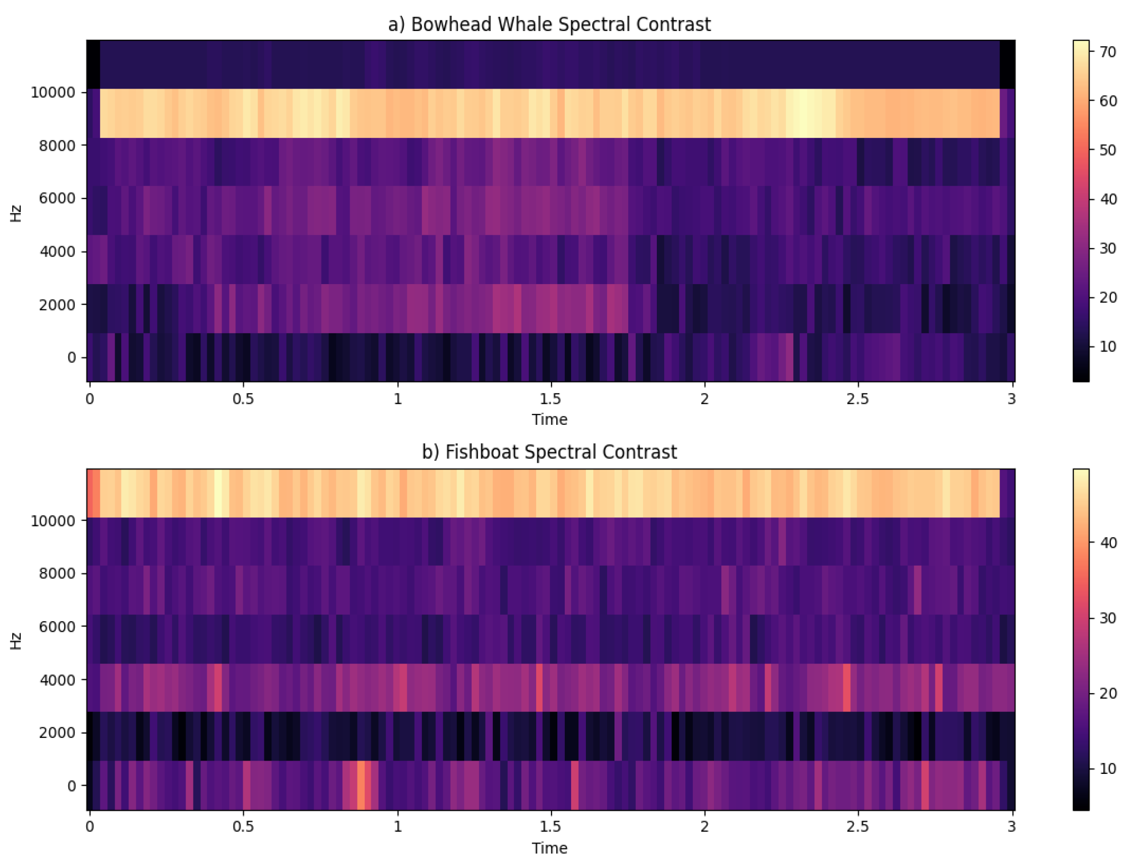
By considering a diverse set of features, including both frequency-based characteristics and temporal dynamics, our approach aims to capture the intricate patterns and relationships present in the audio data. The collaboration of these features contributes to a nuanced understanding of the underlying structure, promoting enhanced interpretability and performance in machine learning models.
The feature extraction functions produces a chromagram, a mel spectrogram, MFCC coefficients, and a Rhythm patterns for each of our audio files. Each function returns a matrix, from which we compute the mean, resulting in a singular feature array for each feature and each audio file. The rhythm pattern generates 340 features. The chromagram yields 12 features, one for each of the 12 pitch classes. The mel spectrogram produces 128 features while 40 coefficients are extracted for the MFCC. In total, we extract 564 features per sample, aligned horizontally in a consolidated feature array. Following this, we applied scaling to our features to ensure proper training of the classifier models. This scaling process includes both min-max and standard normalisation.
4.4. Results
The Table 2 presents the performance metrics of various classifiers across different datasets, focusing on different scaling methods. The datasets are categorized into Mammals, Vessels, and Full Dataset. The classifiers include Support Vector Machine (SVM), Random Forest, KNeighbors, Decision Tree, and AdaBoost. Performance metrics, such as accuracy, are provided for each classifier under the unscaled set, scaled set, and the scaled min-max.
We evaluated classifier performance on various datasets, with a special emphasis on the Full Dataset, Vessels, and Mammals. Among these, the Support Vector Machine (SVM) achieves 99% accuracy on the Full Dataset, which is consistently high. Notably, SVM exhibits robustness and works well in a variety of scaling scenarios. However, Random Forest performs better still, scoring up to 95%, but it is a little more susceptible to changes in scaling. SVM’s dependability is demonstrated by the fact that it performs better than Random Forest in every scaling situation in the Mammals Dataset. These results highlight the significance of taking into account both the classifier selection and the effect of scaling on classification results, with SVM demonstrating to be an especially robust option across a variety of datasets.
5. Discussion
This research presents a comprehensive approach to addressing challenges in passive marine listening, offering an advanced method to enhance the reliability of Mel-frequency cepstral coefficients (MFCCs) amidst the dynamic underwater soundscape. The proposed algorithm, detailed in the study, effectively combines adaptive noise reduction to counter marine noise, showcasing remarkable adaptability to dynamic conditions. The setup, which includes a Raspberry Pi 4, SN005 hydrophones, a floating buoy, and an underwater speaker in a medium-sized pool, provided a controlled environment for the comprehensive evaluations. The algorithm was evaluated through three distinct testing scenarios focusing on marine mammals and vessels identification and classification. Feature engineering process produced results that were instrumental in training classification models, the performance metrics of various classifiers across different datasets highlighted the efficacy of the chosen models. Support Vector Machines (SVM) consistently demonstrated high accuracy, reaching 99% on the full dataset, showcasing robustness across scaling scenarios. Random Forests exhibited good performance, reaching 95% on the full dataset although showed some sensitivity to scaling variations. Effectiveness of Support Vector Machines and Random Forests in the classification of underwater audio is illustrated, offering valuable insights for applications in marine life studies, aquatic event monitoring, and underwater communication research. While this study establishes the efficacy of the proposed algorithm for passive marine listening applications, continued research incorporating more extensive datasets, encompassing a broader range of marine sounds, would contribute to a more robust and versatile algorithm. Furthermore, the controlled environment, while valuable for testing, do not fully capture the complexity of real-world marine soundscapes, deployment in open-water scenarios is already considered to open new avenues for practical implementation.
Funding
This research was funded bythe Chinese Government Scholarship - Chinese University Program grant number 2019DFH011062.
Conflicts of Interest
The authors declare no conflict of interest.
References
- Zunjing Wu and Zhigang Cao, 2005. Improved MFCC-Based Feature for Robust Speaker Identification, Tsinghua Science & Technology, Volume 41,Volume 10, Issue 2, Pages 158-161, ISSN 1007-0214. [CrossRef]
- Wei Han, Cheong-Fat Chan, Chiu-Sing Choy and Kong-Pang Pun, 2006. An efficient MFCC extraction method in speech recognition, 2006 IEEE International Symposium on Circuits and Systems (ISCAS), Kos, Greece, 2006, pp. 4 pp.-. [CrossRef]
- S. Lalitha, D. Geyasruti, R. Narayanan, Shravani M, 2015. Emotion Detection Using MFCC and Cepstrum Features, Procedia Computer Science, Volume 70, Pages 29-35, ISSN 1877-0509. [CrossRef]
- A. Milton, S. Sharmy Roy, S. Tamil Selvi, 2013. SVM Scheme for Speech Emotion Recognition using MFCC Feature, International Journal of Computer Applications, (0975 – 8887) Volume 69– No.9.
- Chang-Hsing Lee, Chih-Hsun Chou, Chin-Chuan Han, Ren-Zhuang Huang, 2006. Automatic recognition of animal vocalizations using averaged MFCC and linear discriminant analysis, Pattern Recognition Letters, Volume 27, Page 93–101. [CrossRef]
- JLin Shi, Ishtiaq Ahmad, YuJing He and KyungHi Chang, 2018. Hidden Markov Model based Drone Sound Recognition using MFCC Technique in Practical Noisy Environments, JOURNAL OF COMMUNICATIONS AND NETWORKS, VOL. 20, NO. 5. [CrossRef]
- Juan J. Noda, Carlos M. Travieso-González, David Sánchez-Rodríguez and Jesús B. Alonso-Hernández, 2016. Acoustic Classification of Singing Insects Based on MFCC/LFCC Fusion, Applied Sciences, Volume 9, 4097. [CrossRef]
- Muqing Deng, Tingting Meng, Jiuwen Cao, Shimin Wang, Jing Zhang, Huijie Fan, 2020. Heart sound classification based on improved MFCC features and convolutional recurrent neural networks, Neural Networks, Volume 130, Page 22–32. [CrossRef]
- Nsalo Kong, D.F.; Shen, C.; Tian, C.; Zhang, K, 2021. A New Low-Cost Acoustic Beamforming Architecture for Real-Time Marine Sensing: Evaluation and Design, Journal of Marine Science and Engineering, 9, 868. [CrossRef]
- William A. Watkins, n.d. Watkins Marine Mammal Sound Database/New Bedford Whaling Museum, Woods Hole Oceanographic Institution, accessed 16 April 2023, https://whoicf2.whoi.edu/science/B/whalesounds/index.cfm.
- David Santos-Domínguez, Soledad Torres-Guijarro, Antonio Cardenal-López, Antonio Pena-Gimenez, 2016. ShipsEar: An underwater vessel noise database, Applied Acoustics, Volume 113,Pages 64-69,ISSN 0003-682X. [CrossRef]
- A.Harma, 2003. Automatic identification of bird species based on sinusoidal modeling of syllables, Internat. Conf. on Acoust. Speech Signal Process. 5, 545–548.
- Pedregosa, F. and Varoquaux, G. and Gramfort, A. and Michel, V. and Thirion, B. and Grisel, O. and Blondel, M. and Prettenhofer, P.and Weiss, R. and Dubourg, V. and Vanderplas, J. and Passos, A. and Cournapeau, D. and Brucher, M. and Perrot, M. and Duchesnay, E., 2011. Scikit-learn: Machine Learning in Python, Journal of Machine Learning Research, 12, 2825–2830. [CrossRef]
Figure 1.
Overall flowchart of the proposed method.
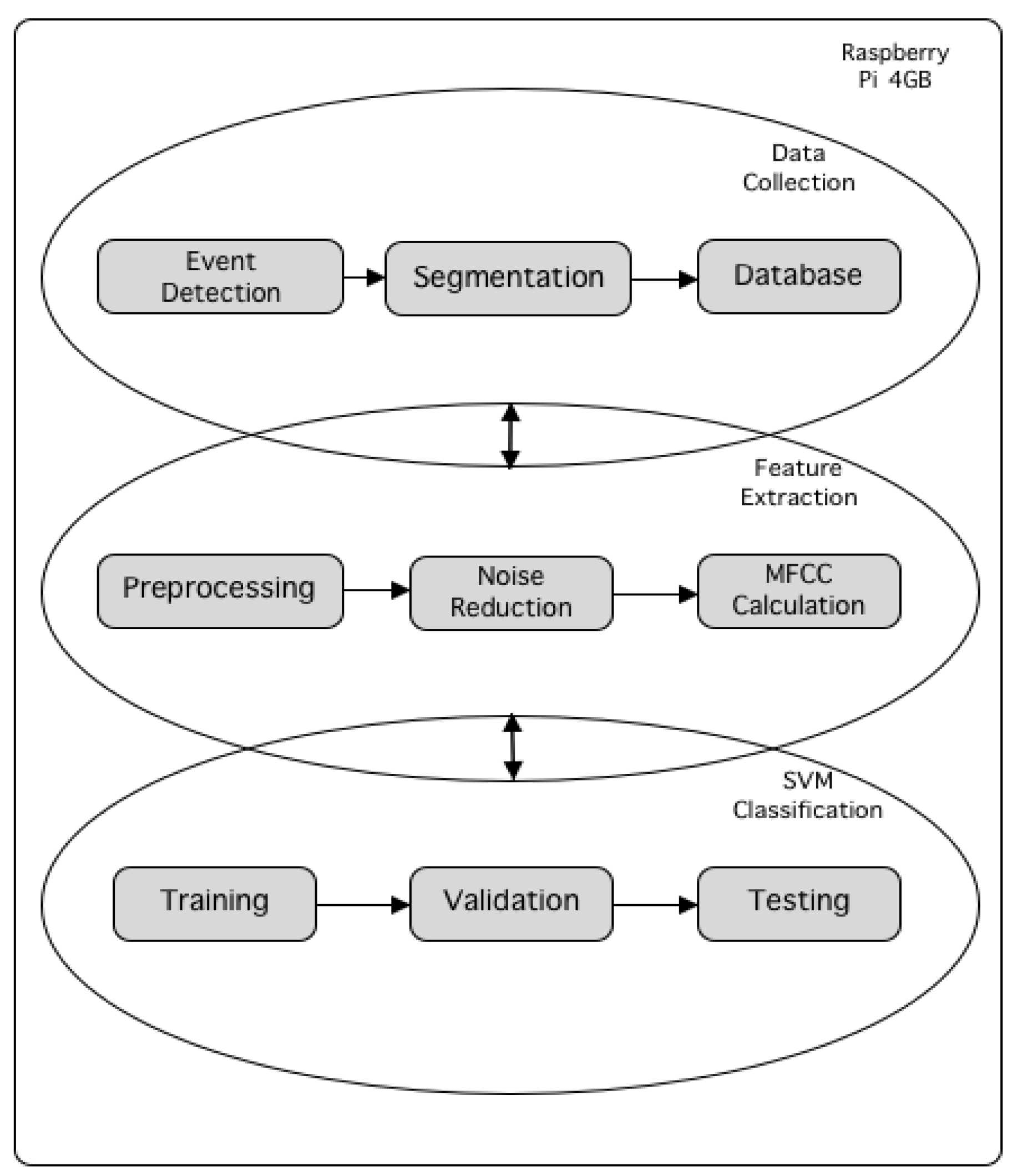
Figure 2.
Experiment Setup.
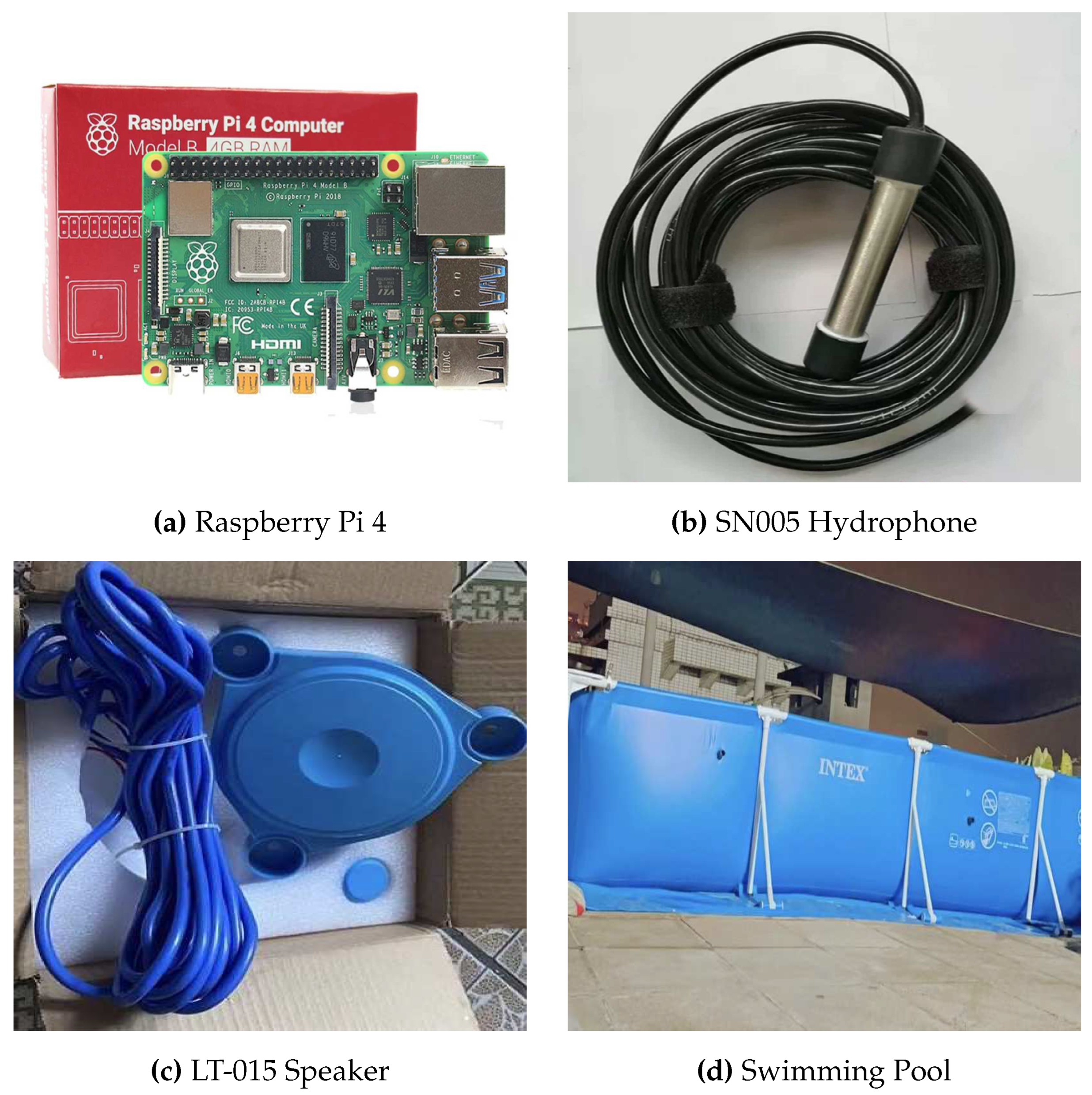
Figure 3.
Mel-Frequency Cepstral Coefficients (MFCC).
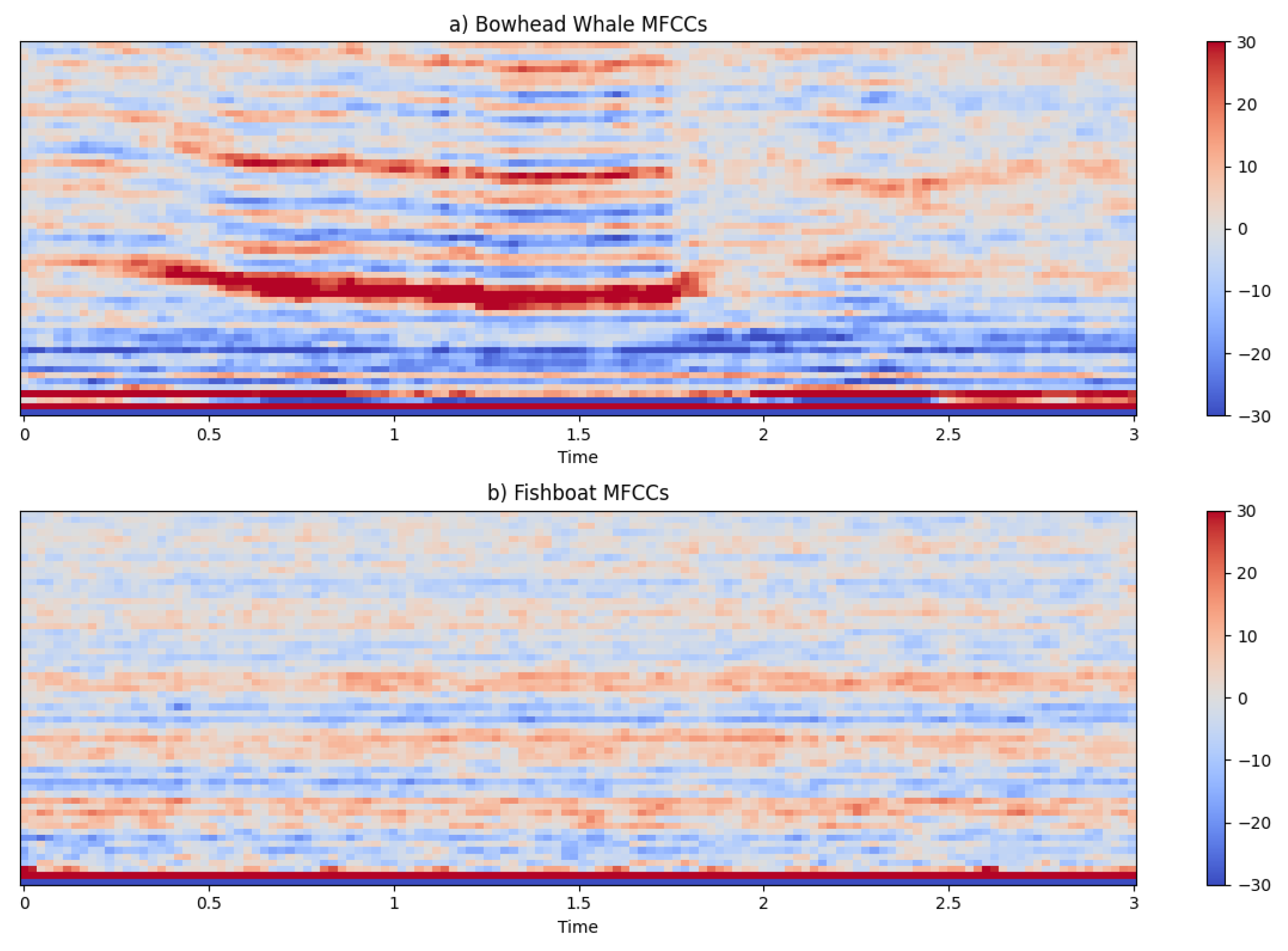

Table 1.
Data Split for Training, Validation, and Testing Sets.
| Class | Type | Training | Validation | Testing | Total |
|---|---|---|---|---|---|
| Mammal | Atlantic Spotted Dolphin | 9 | 3 | 3 | 15 |
| Mammal | Bearded Seal | 9 | 3 | 3 | 15 |
| Mammal | Beluga, White Whale | 9 | 3 | 3 | 15 |
| Mammal | Bottlenose Dolphin | 9 | 3 | 3 | 15 |
| Mammal | Bowhead Whale | 9 | 3 | 3 | 15 |
| Mammal | Clymene Dolphin | 9 | 3 | 3 | 15 |
| Mammal | Common Dolphin | 9 | 3 | 3 | 15 |
| Mammal | False Killer Whale | 9 | 3 | 3 | 15 |
| Mammal | Fin, Finback Whale | 9 | 3 | 3 | 15 |
| Mammal | Fraser’s Dolphin | 9 | 3 | 3 | 15 |
| Mammal | Grampus, Risso’s Dolphin | 9 | 3 | 3 | 15 |
| Mammal | Harp Seal | 9 | 3 | 3 | 15 |
| Mammal | Humpback Whale | 9 | 3 | 3 | 15 |
| Mammal | Killer Whale | 9 | 3 | 3 | 15 |
| Mammal | Leopard Seal | 9 | 3 | 3 | 15 |
| Mammal | Long-Finned Pilot Whale | 9 | 3 | 3 | 15 |
| Mammal | Melon Headed Whale | 9 | 3 | 3 | 15 |
| Mammal | Minke Whale | 9 | 3 | 3 | 15 |
| Mammal | Narwhal | 9 | 3 | 3 | 15 |
| Mammal | Northern Right Whale | 9 | 3 | 3 | 15 |
| Mammal | Pantropical Spotted Dolphin | 9 | 3 | 3 | 15 |
| Mammal | Ross Seal | 9 | 3 | 3 | 15 |
| Mammal | Rough-Toothed Dolphin | 9 | 3 | 3 | 15 |
| Mammal | Short-Finned (Pacific) Pilot Whale | 9 | 3 | 3 | 15 |
| Mammal | Southern Right Whale | 9 | 3 | 3 | 15 |
| Mammal | Sperm Whale | 9 | 3 | 3 | 15 |
| Mammal | Spinner Dolphin | 9 | 3 | 3 | 15 |
| Mammal | Striped Dolphin | 9 | 3 | 3 | 15 |
| Mammal | Walrus | 9 | 3 | 3 | 15 |
| Mammal | Weddell Seal | 9 | 3 | 3 | 15 |
| Mammal | White-beaked Dolphin | 9 | 3 | 3 | 15 |
| Mammal | White-sided Dolphin | 9 | 3 | 3 | 15 |
| Vessel | Dredger | 9 | 2 | 2 | 13 |
| Vessel | Passengers | 18 | 6 | 6 | 30 |
| Vessel | Ocean liner | 4 | 2 | 2 | 7 |
| Vessel | Motorboat | 11 | 4 | 4 | 19 |
| Vessel | Fishboat | 5 | 2 | 2 | 9 |
Table 2.
Classifier Performance on Different Datasets.
| Dataset | Classifier | Performance Metrics | ||
| Unscaled Set | Scaled Set | Scaled Min-Max | ||
| SVM | 0.99 | 0.99 | 0.98 | |
| Random Forest | 0.93 | 0.95 | 0.89 | |
| Full Dataset | KNeighborst | 0.69 | 0.72 | 0.65 |
| DecisionTree | 0.75 | 0.77 | 0.72 | |
| AdaBoost | 0.56 | 0.79 | 0.62 | |
| SVM | 0.85 | 0.87 | 0.83 | |
| Random Forest | 0.76 | 0.84 | 0.66 | |
| Mammals | KNeighbors | 0.50 | 0.62 | 0.42 |
| DecisionTree | 0.67 | 0.67 | 0.63 | |
| AdaBoost | 0.09 | 0.55 | 0.09 | |
| SVM | 0.82 | 0.84 | 0.82 | |
| Random Forest | 0.75 | 0.76 | 0.69 | |
| Vessels | KNeighbors | 0.50 | 0.61 | 0.55 |
| DecisionTree | 0.65 | 0.69 | 0.67 | |
| AdaBoost | 0.09 | 0.09 | 0.09 | |
Disclaimer/Publisher’s Note: The statements, opinions and data contained in all publications are solely those of the individual author(s) and contributor(s) and not of MDPI and/or the editor(s). MDPI and/or the editor(s) disclaim responsibility for any injury to people or property resulting from any ideas, methods, instructions or products referred to in the content. |
© 2024 by the authors. Licensee MDPI, Basel, Switzerland. This article is an open access article distributed under the terms and conditions of the Creative Commons Attribution (CC BY) license (http://creativecommons.org/licenses/by/4.0/).
Copyright: This open access article is published under a Creative Commons CC BY 4.0 license, which permit the free download, distribution, and reuse, provided that the author and preprint are cited in any reuse.


