
Submitted:
08 January 2024
Posted:
08 January 2024
You are already at the latest version
Abstract
The container relocation problem (CRP) is one of the important topics in container terminals, which aims to find the optimal sequence of movements to minimize the total number of relocations needed to retrieve all the containers within a bay according to a given specific layout and retrieval order. However, determining such an order may be difficult due to uncertainty. Various CRP solution methods proposed so far show a common pitfall concerning the complexity of the solving process, whose scale grows exponentially with the number of containers. Considering the retrieval operation process of the inbound containers in a bay consists of several operation rounds, this paper focuses on the real-time operation scenario of each round to minimize the actual number of relocations during the pick-up process, i.e., starting from the initial layout of the bay, we minimize the sum of the incremental number of blocking containers due to the layout change and the number of reallocated containers unrelated to the target container. We present a heuristic algorithm (called SPFH) based on the three rules (LL, MSS, and FSS), considering the adjustment of the pick-up order of containers. Numerical experiments on a set of instances generated from the literature are performed. The proposed methodology excels in both execution efficiency and solution quality and is capable of solving instances that were impossible to solve before. This also makes our methods appealing for being applied in practice. The source codes are available at https://github.com/zhou-sf/rt-scrp.
Keywords:
Container Relocation Problem
; Stochastic Container Relocation Problem
; Real-Time Batch Optimization
; Heuristics
1. Introduction
Generally, in the yard of the container terminal, containers are stacked on top of each other in the ground slots, forming stacks. At the same time, a row comprises several stacks placed abreast, constituting a bay, and each yard block is composed of dozens of bays. The containers in a stack adhere to the last-in-first-out (LIFO) principle. If a target container that needs to be retrieved is not the topmost in its stack and is covered by other containers, the blocking containers must be moved to another stack in the same bay first. As a result, the yard crane is required to perform one or more relocation movements. Moving a blocking container, referred to as relocation (rehandling or reshuffling), is an unproductive operation. A high proportion of unproductive operations resulting from container rehandling decreases yard operational efficiency, delays the turnaround time of external trucks, and increases the detention time of vessels. Thus, the container relocation problem (CRP) is a significant source of inefficiency in container terminals and has received considerable attention from terminal operators and scholars.
The CRP aims to find optimal yard crane operation plans for retrieving all the containers in a bay while minimizing the number of relocations. Consequently, the CRP model needs to explore all operation options to find the optimal solution, resulting in an exponential increase in computational effort as the number of containers increases. As an NP-hard problem Caserta et al. [1], it means that it is difficult to obtain an optimal solution for a large-scale instance because it is very time-consuming. Comparatively, getting the approximate optimal solution using heuristic algorithms is valuable and more efficient. Many heuristics, such as ERI ([2]), Chain-LAN ([3]), LA-N ([4]), GLAH ([5]), are outstanding in solving the CRP. However, these heuristics are built based on clear retrieval sequences and may not apply to the relocation problem with uncertain retrieval orders. The main challenge and complexity of the CRP for inbound containers are that it is difficult to accurately master the retrieval order of containers in advance since the arrival time of trucks is random[6]. The uncertainty of the retrieval order of inbound containers makes the CRP for inbound containers intractable.
Stochastic container relocation problem (SCRP) is a CRP variant for inbound containers, also called a CRP with time windows. In the SCRP, the containers are divided into different batches (groups) according to their departure time window, i.e., a batch of containers indicates that the set of containers is stacked in the same bay and with the same retrieval time window. Usually, the retrieval time window is obtained from the truck appointment system (TAS), which has recently been implemented in many container terminals. Containers are ordered so that all containers in a batch must be retrieved before any containers from a later batch. Furthermore, the relative retrieval order of containers within a given batch is assumed to be a random permutation [2,7,8,9]. So, the SCRP is dedicated to retrieving all the containers in a bay while minimizing the expected number of relocations during the pick-up operation process.
Due to the uncertainty of the arrival time of the external trucks and the limited number of yard cranes, the pick-up operation process of inbound containers in a bay can be regarded as a multi-round process. If an external truck (ET) has arrived at the terminal and there is no yard crane to serve the destination bay, the ET must wait until a yard crane is moving into the destination bay to complete pick-up and departure. As shown in Figure 1 (a), we define an operation round as the bay is in busy state, whose period that begins when the yard crane moves into the destination bay and ends when the yard crane moves out the destination bay. Figure 1 (b) tells us that the whole retrieval process of a bay can be divided into three parts — completed operation rounds, real-time operation rounds and future operation rounds. The completed operation rounds represent that the retrieval and relocation operations have been finished, which is irreversible. The real-time operation round refers to when a yard crane provides a loading service for the waiting ETs. The operations within the real-time operation round are unrelated to the completed operation round but will impact future operations.
In this study, a new perspective, namely the Real-time Batch Optimization method, is proposed for dealing with the SCRP during the retrieval process of inbound containers. The new perspective guides us to focus on optimizing the real-time operation round and constructing the evaluation function for evaluating the expected increment of the number of blocking containers with the bay layout change instead of exploring the subsequent operation processes to improve the solution efficiency. In the new approach, we first categorize the ETs into batches (groups) based on their reservation information from the TAS, as in the existing literature. Of course, the retrieval sequence of the ETs belonging to different batches is precise, and the retrieval sequence of the ETs within the same batch is still being determined. Then, based on this grouping, all the arrived ETs within the real-time operation round are defined as a specific batch (group) whose retrieval priories are set to zero, representing the highest pick-up priority. Correspondingly, the target containers within the real-time operation round are a batch with a retrieval priority of 0, which may only be part of the containers booked in the current time window. Moreover, their pick-up service order of all arrived ETs is adjustable (no longer following the first-come-first-served principle), and the optimal pick-up order is determined based on the bay layout to minimize the number of relocations.
The contributions of this paper are as follows:
- We derive an improved dynamic programming (DP) model for the real-time retrieval operation scenarios of SCRP. Compared to the general SCRP, this improved DP model focuses on optimizing the real-time operation round and less explores the future operation processes.
- We introduce two novel relocation rules: moving ahead for a sequential-placed slot (MSS) and freeing up for a sequential-placed slot (FSS). The former rule assigns, as far as possible, a sequential placement for the potential blocking containers in the future in advance. The latter rule tries to find a stack that can free its topmost container to satisfy a sequential placement for the current blocking container.
- A novel heuristic algorithm, called the sequential-placement first heuristic (), is devised. It takes advantage of the properties of the two relocation rules mentioned above. The algorithm is explained with pseudo-code in Algorithm 3.
The rest of the paper is structured as follows: In Section 2, we quickly survey recent literature on the CRP. Section 3 gives a detailed description of the real-time CRP and the formulation of the improved DP model. Section 4 describes the proposed algorithm in detail. We report the results of our computational experiments with the methods discussed in this paper in Section 5. Finally, Section 6 concludes the study and suggests future research directions.
2. Literature Review
Two fields have been extensively investigated in the existing literature to reduce relocations during the retrieval process of inbound containers. In the first field, the objective is to allocate stacking locations for new unloaded containers to reduce relocation moves in the future. Such as, the formulations for evaluating the expected number of rehandles were proposed in [10,11] based on the segregation storage strategies. Other similar studies on generating container storage strategies can be found in [12,13,14]. The second field, also known as the container relocation problem, focuses on the relocation movements during the retrieval process and is aimed at deciding to which stack the blocking containers should be moved to be considered to reduce the relocations.
Due to the containers stacked on top of each other and the limited yard area, the relocating operation is unavoidable in the container terminal yard. So, the CRP has received much attention from scholars for decades. Various integer programming (IP) or mixed-integer programming (MIP) models [see, e.g., [15,16,17,18,19] and exact algorithms based on tree search procedures have been developed, such as tree search algorithms [20,21,22], beam search algorithms [23], (iterative deepening) A* algorithms [24,25], B&B algorithms [19,21,26,27,28,29,30,31], and abstract approaches [2]. However, the CRP is an NP-hard problem. For larger-scale instances, the exact algorithms or models mentioned above are time-consuming and impractical for real-time operation demands. Therefore, researchers have been increasingly exploring heuristic algorithms to overcome the computational complexity of CRP. So far, many outstanding heuristic algorithms have been developed, such as beam search algorithms [23,28,29,31], greedy heuristics [3,5,32], and other heuristics based on relocation rules [2,8,9,21].
In the earlier literature, due to the difficulty of obtaining the retrieval time information in advance, some studies constructed random models for CRP based on assuming that the retrieval processes of the inbound containers conform to some probability distribution [15,33,34]. Moreover, some papers proposed the online CRP models, where the retrieval orders of the containers are revealed progressively with the arrival of ETs [2,7,8]. Truck appointment systems (TAS) allow terminal operators to obtain the containers’ retrieval time window through the TAS. Based on the appointment information, some researchers proposed batch model where the containers within the same appointment time windows are considered a batch. Based on the batch model, [9] proposed the stochastic container relocation problem (SCRP), where the retrieval order between different batches is clear but uncertain within the same batch. It means the containers within the same batch have the same retrieval probability. Indeed, the retrieval sequence of the same batch containers is indistinguishable until associated ETs arrive.
For the CRP, relocating operations occur when the container pick-up orders do not match their stacking sequence. Many studies address the container storage allocation/re-allocation problem, but only some focus on controlling the retrieval sequence. [7] first proposed an embryo of the Batch Optimization method, in which a batch of ETs has arrived, and their pick-up service orders are adjustable. Nevertheless, they only apply this method to the first batch to avoid delaying the other ETs’ waiting time. [?] proposed a rehandling model that considered adjustments to the container pick-up order within each group to minimize the number of rehandles. They grouped the ETs according to the appointment time slots in the TAS. [6] proposed a flexible service policy for the SCRP, which assumes all the ETs corresponding to the containers of each batch arrived in advance and dictates the retrieval orders of the current batch’s inbound containers to minimize the number of relocations. In practice, some arriving ETs within a real-time operational round are likely different from their reservations. Therefore, the abovementioned studies need more practicality and flexibility in real-time operation scenarios. However, they show us a novel optimization perspective on the CRP. So far, there is little literature discussing the novel perspective. Summarily, the batch optimization method has two important features—certainty (the arrival of ETs means that the corresponding target containers of a batch have been identified) and flexibility (the pick-up order of the containers of a batch is adjustable).
The novelty of this work. Compared with the previous studies, our paper proposes a new perspective on studying the real-time operation scenario for the SCRP. In our work, we formulate a new dynamic programming model and develop a novel heuristic algorithm, which performs better on the runtime and solution quality than existing outstanding heuristics.
3. Problem description and formulation
3.1. Retrieval process analysis
Due to the limited number of yard cranes, each must move back and forth between different bays rather than being dedicated to a specific unit. When a truck arrives, the yard crane may not serve the destination bay immediately. In such cases, the ETs must wait until a yard crane enters the destination area. As shown in Figure 1, the operation state of a bay changes as the yard crane moves in or out. When the yard crane moves in the bay, its operation state changes into busy, i.e., the bay begins its real-time operation round. When the yard crane moves out of the bay, it implies that the real-time operation round has finished and changed into the completed operation round. Meanwhile, the bay state changes into idle.
Consider a bay with N containers piled on W stacks, and the height of each stack cannot exceed H tiers. In the initial state, all the N containers in the bay have been appointed their departure time windows according to the corresponding ETs’ reservation arrival period. In turn, they can be classified into G groups based on their respective booking departure times and numbered , which implied their retrieval priorities (the smaller group index, the higher retrieval priority).
Suppose this instance requires K () operation rounds to finish retrieving all the N containers. Let denote the bay layout after the completion of kth operation round, especially indicating the initial layout when . Suppose we have completed the first operational rounds, and then we need to complete the kth operation round. We aim to find an optimized solution for the kth operation round that minimizes the number of relocations during the kth operation round. Once the kth operation round finishes, the bay layout will be transformed from to , which becomes the basis for th operation round. The change of the bay layout between two adjacent operation rounds is described by the following equation 1.
The is a set of operation instructions. If includes some relocation operation instructions, some containers will be moved from their stacks into other new stacks. For the restricted CRP, the relocated containers are only the blocking containers above the targets. The relocated containers may contain containers other than the blocking containers above the targets for the unrestricted CRP. However, these movements may result in the addition of the number of blocking containers for the moved-in stacks and impact the th and subsequent operation rounds. Our objective is to minimize the addition of the number of blocking containers in the real-time operation round.
Moreover, during real-time operations, the retrieval sequence of target containers and the movement orders of blocking containers determine the changes in the bay layout, and different bay layouts will produce different increments in the number of blocking containers and other impacts on the subsequent operation process. In the real-time operation round, when multiple target containers need to be picked up, it makes sense to choose a reasonable target container pick-up order that can produce fewer relocation operations, even though it may prolong the waiting time of some ETs. Therefore, the method proposed in this paper allows for adjusting the pick-up order according to the bay layout, integrating the optimization of the pick-up sequence and the reallocations of blocking containers to minimize the increment of the expected number of blocking containers (ENBC). No doubt, the pick-up order in practice is likely to be inconsistent with the ETs’ arrival sequences, which will result in loading operations being advanced for some ETs and delayed for others. In practice, the number of waiting ETs for retrievals is usually small, and as the number of relocations decreases, the whole operation time decreases, and the delays incurred by individual ETs are acceptable.
3.2. Formulation for the real-time scenario of CRP
Learning from [2], we first present a simplified DP model of real-time CRP. Let denote the minimum number of relocations required to remove all the remaining containers based on the layout , and let denote the number of realized operations that occur during the kth operation round. The DP model can be formulated as a recursive function as in Eq. (2).
From Eq. (3), to obtain the optimal operation plan for the kth operation round, the solution process requires simultaneous evaluation of the optimal operation plan from the th operation round to the last operation round. So, solving the total optimization objective , which is the minimum number of relocations for picking up all containers during the whole retrieval process, is difficult because the complete solving process will generate a large number of redundant computation efforts. Consider it another way, and we can try to find an approximate optimal solution for it.
According to the Eq. (2), if is the theoretically optimal operation plan for the kth round, then we have . Since solving for the theoretical optimum is difficult, assuming that we get an approximate optimal solution for the kth operation round, we can derive an inequality Eq. (4).
Without loss of generality, if are approximate optimal solutions for each round, respectively, then we must have inequality Eq. (5).
In this way, we convert the solving process of Eq. (3) to summing the number of practical relocations during each operation round. We can ensure the desired suboptimal solution if we minimize the number of relocations within each round and the impact on the subsequent operation rounds.
According to the definition, includes two aspects: forced relocations and relocations to free up storage placements. The forced relocations result from blocking the target containers during the real-time operation round. The relocations to free up storage placements result from the containers having nothing to do with the target containers and aim to free up good placements for the blocking containers. In addition, some blocking containers may be relocated twice or more due to all candidate storage positions containing the target containers, but this case is included in the forced relocations. Therefore, we can derive the following inequation as Eq. 6.
denotes the blocking containers of the target container c in kth operation round, and means the set of relocated containers not within the same stack as the target containers during the kth operation round.
Let denote the number of blocking containers in the layout , which will require rehandling operations in the remaining rounds. indicates the set of target containers in kth operation round. During the kth operation round, Each container must be moved into other stacks and may become new blocking containers in the move-in stack. Let denote the expected additional number of the blocking containers when the container b is moved into the stack s. Its formula will be given later. Thus, after completing the kth operation round, the number of blocking containers in the layout is as Eq. 7.
When we have removed all the containers, the last bay layout is empty and . Iterative summation of Eq. 7 for k from 1 to K yields Eq. 8.
The total optimizing objective of this study is . It satisfies inequality Eq.9.
The initial layout of a bay is fixed, and the can be considered a constant. According to Eq. (9), a suboptimal solution to the CRP can be obtained by minimizing the expected increment in the number of blocking containers and the number of rehandles due to relocations within each operating round. Therefore, we concentrate on optimizing the real-time operation process of each round and decrease the computational efforts for assessing the influence of relocating obstructive containers within each round on subsequent operation rounds. This method will significantly enhance the solution efficiency of the CRP and make it suitable for real-time scenarios.
4. Algorithm design
According to Eq. (9), the real-time scenario of the CRP focuses on two aspects: (1) Minimizing the instant relocation number during the real-time operation round; (2) Minimizing the incremental number of the blocking containers after each operation round.
4.1. Preliminaries
Before describing the implementation of the algorithms in detail, we first define the placement state of containers and then introduce three heuristic relocation rules.
4.1.1. Placement state of containers
Let represent the retrieval priority value of container c and denote the minimum retrieval priority value of the container set s (If s is a stack number, it represent all the containers in stack s), the smaller value, the higher priority. Specifically, if s is an empty set or stack. Let denote the containers set within the same stack with container c and below it.
We define three placement state types of containers as follows. The placement state of the container c is to be known as: (1) sequential-placement if is satisfied; (2) inverted-placement if is satisfied; (3) level-placement if is True. A sequential-placement container means that all other containers placed below have lower retrieval priorities than it. Similarly, an inverted-placement container means that all other containers placed below have higher retrieval priorities than it, i.e., it has a bigger retrieval priority value than the other containers below it. A level-placement container has the same retrieval priority as the highest retrieval priority of the other containers placed below.
4.1.2. The evaluation method of ENBC
Based on their predetermined precedence (e.g., appointment time window), the containers with higher precedence will be retrieved earlier than those with lower precedence during retrievals. Therefore, a sequential-placement container will be picked up earlier than other containers below it without relocation. Conversely, an inverted-placement container must be relocated at least once, as some containers below it will be picked up earlier. We assume the containers with the same retrieval priority have the same retrieval probability. So, a level-placement container causes a relocation when the same retrieval priority container below it is picked up earlier. The blocking containers in a bay layout include the inverted-placement and level-placement containers, and the ENBC is equal to the sum of the number of inverted-placement containers and the expected relocation number of the level-placement containers. The calculation method for the ENBC can be described as Eq. (10), which has been investigated in [9]. In Eq. (10), is an indicator function that equals one if x is True and zero otherwise, and indicates the container number within stack r.
There is no increase in the number of blocking containers in a candidate stack when a blocking container becomes a sequential-placement container after being moved into the candidate stack during retrieval. We refer to the candidate stacks for the blocking container that satisfy the above condition as sequential-stack (SS for short). Contrarily, the ENBC of the candidate stack will increase when a blocking container becomes the inverted-placement or level-placement container after being moved into a candidate stack. The candidate stack that satisfies the condition is referred to as inverted-stack (IS for short) or level-stack (LS for short), respectively. The notation has been defined previously, which denotes the increment of ENBC of the stack r after relocating the container c into stack r, and the formula is shown Eq. (11).
Where denotes the number of containers with the same priority as container c in the stack r.
4.1.3. Heuristic relocation rules
We introduce three relocation rules in this subsection. The first relocation rule, namely the Least-relocations-and-Lowest-precedence-gap (LL) rule, draws inspiration from relocation rules such as ERI [2], Minmax [35], and EM [9]. The other two relocation rules are used to compensate for the deficiencies of the LL rule, including the prospective re-allocations for some non-instant-relocated blocking containers to produce a better layout.
LL rule
Two conditions construct the LL rule. They are first, selecting the set of stacks that produces the smallest increment of the ENBC after reshuffles—second, choosing the move-in stack from the set of stacks obtained in the “first step” with the closest priority value for the blocking container. Eq. (12) describes the mathematical formula of the LL rule.
denotes the function to get the stack index where the container c is stacked. If , it indicates that the topmost slot of stack is a sequential stack for blocking container c. Therefore, moving container c to stack does not increase the ENBC. If , it indicates that there is no sequential stack for blocking container c to move in. The LL rule provides a method for selecting the move-in stack for container c, which suggests that the stack with the closest precedence to container c is the best choice. This rule has the advantage of keeping the stack with lower priority to provide sequential stacks for subsequent blocking containers as much as possible. Figure 2 illustrates an example of the LL rule.
The rule has two potential areas for improvement. Firstly, it is a greedy approach that always assigns a sequential placement for the relocating container whenever possible, which will likely trap into the local optimum. In other words, reallocating a blocking container with higher retrieval priority to a sequential placement with lower priority may result in losing sequential-placed slots for subsequent relocations. Secondly, when only inverted-placement slots are available for the blocking container, the subsequent blocking containers likely have no more sequential placements to select from, which will directly make additional relocations or result in more potential relocations in the following retrieval processes. The next two relocation rules remedy the deficiencies of the rule in the previously mentioned aspects.
Moving ahead for Sequential Stack (MSS)
Given the blocking container c that is next to be relocated, its optimal reallocation stack is determined according to the rule. If stack is sequential-stack for blocking container c, we try to find another inverted-placement container, which is the topmost item in its stack s () and denotes as . If stack is sequential-stack for container and moving it into stack before container c does not change the sequential-placement state of container c. We define this method as a relocating policy, known as the Moving-ahead for Sequential Stack (MSS) rule. The MSS rule aims to move a inverted-placement container into a sequential-stack stack in advance and reduce the likelihood of the container becoming a blocking container again in the subsequent operation process. This rule needs to comply with the following conditions: (1) There are at least two empty slots in stack ; (2) The topmost container in stack s must be in inverted-placement state, i.e., its retrieval priority satisfies the condition . (3) the retrieval priority of container must satisfy the condition , i.e., the stack is sequential-stack for containers c and and the retrieval priority of container is lower than container c. Figure 3 illustrates the processing procedure of the MSS rule.
Freeing up for Sequential Stack (FSS)
For a blocking container c, if only inverted-stack stacks are available, directly moving container c into one of the stacks will add a new blocking container and, in turn, add a relocation during the subsequent retrieval processes. In this case, selecting a suitable stack s and moving its topmost container to another stack will free up an sequential-placement for container c. If stack is a sequential-stack for container , the total operation cost of the “free up” operations is the same as that of direct moving. As well as it may also increase the possibility of selecting sequential-placement for the subsequent relocations. We refer to the above method as a new relocation policy: freeing up for the sequential stack (FSS) rule. The FSS rule needs to comply with the following conditions: (1) The available reallocation positions for the blocking container c are inverted-placements; (2) If stack s is a candidate sequential-placement for the blocking container c by freeing up the topmost item , while the retrieval priority value satisfies . (3) The container will be moved into stack , which must be the sequential-stack for container .
We now continue to analyze the instance depicted in Figure 4. In the final configuration, container is the current forced relocating item, and two available stacks, the second and fourth stack, are both inverted stacks. Let us move container from the fourth to the second stack and obtain a sequential stack by consuming one practical relocation movement. Furthermore, this reshuffle is cost-effective since it may provide an additional sequential-placement in subsequent processes. Figure 4 illustrates the detailed processing of the FSS rule.
4.2. sequential-placement first heuristic ()
This section presents the algorithm for the real-time operation round of SCRP. The algorithm structure of includes two levels. The outer level adopts a policy iteration mechanism, i.e., the set of policies comprising all possible pickup sequences, from which the best operation solution has the least cost; the inner level is the specific process of simulating the operation solution and evaluating the cost for each pickup sequence.
4.2.1. The Outer Level of
takes two inputs: denotes the initial configuration of the current operation round of the bay, and P denotes the target container set of the current operation round. In the outer level of , the procedure, namely AutoRetrieval, is a conventional prioritization mechanism that checks and automatically picks up the target containers if retrievable before the start of each operation round or after each relocation. This mechanism makes the configuration irreducible while freeing up optional slots for other blocking containers. The procedure, namely GenerateSequence, generates all possible pickup orders for the target containers of the current operation round. Then, iterate these orders to obtain the best operation plan for the yard cranes with minimal operation costs. The procedure, namely Simulation-Evaluation, is the inner level of the algorithm. The pseudo-code of the outer level of is shown in Algorithm 1, and the pseudo-codes of the procedure AutoRetrieval and the procedure GenerateSequence are shown in Algorithm 2.
| Algorithm 1 Outer level: the main procedure of algorithm |
|
| Algorithm 2 The procedures: AutoRetrieval and GenerateSequence |
|
4.2.2. The Inner Level of SPFH
The objective of the inner level of SPFH is to simulate the relocation operation processes and estimate the associated operation costs concerning a given pickup sequence. This procedure involves removing the target containers of the current operation round and moving their blocking containers into the best placements with the least cost (the sum of the number of instant relocation moves and the addition of ENBC).
The detailed simulation and evaluation procedure consists of the following steps. Firstly, we apply the LL rule to identify the optimal stack , which will minimize the addition of ENBC among all assignable slots to which we can move the blocking container directly. However, the earlier reallocations of the blocking containers occupy reasonable placements and may lead subsequent blocking containers to lose the well-stacking slots. Hence, we will consider the impact of current reallocation decisions on subsequent blocking containers and determine whether there are better solutions than the current selection. Suppose the selected stack is a sequential-stack for the current blocking container. In this case, we will check for some inverted-placement containers that satisfy the MSS rule to increase the chances of choosing a well-stacking position for other blocking containers. Similarly, suppose the selected stack is a inverted-stack, we will try to find a stack satisfying the FSS rule that the stack is a sequential-stack for the current blocking container after moving the topmost container in stack to another stack. The optimal result is that the non-forced relocating container obtains a new well-stacking placement. Otherwise, relocating the non-forced container will increase the final operational cost in the future. Moreover, when stack provides a level-placement for the current relocating container, neither the MSS rule nor the FSS rule is applicable because they may exacerbate the problem. Algorithm 3 presents the pseudo-code for the inner level of .
| Algorithm 3 Inner level: Policy iteration procedure |
|
5. Computational Experiments
In this section, we present some computational experiments to validate the effectiveness of the heuristic and algorithm for the real-time operations of SCRP.
5.1. Implementation details
Our experiments are implemented by Matlab 2016b and conducted on a PC with an Intel Core I7-9700K CPU at 3.6GHz and 16GB RAM. The program code, results and instances used in this section are available at https://github.com/zhou-sf/rt-scrp. We generate our experiment dataset based on the existing dataset from [9] and complete our experiments from four cases. Each case of the experiments is implemented with 30 instances. We consider the heuristic as a standalone algorithm for comparison experiments.
Our experiments validate the effectiveness and performance of the LL heuristic and algorithm under small-batch and large-batch instances, respectively. In the case of small-batch instances, the configuration sizes of the instances vary from stacks and tiers and batch sizes of each operation round vary from containers. The configuration sizes of the large-batch instances vary from stacks and tiers, and batch sizes of each operation round vary from containers.
5.2. Experiment results
5.2.1. Effectiveness validation under small-batch instances
36 configurations, each of 30 instances, are solved using the proposed heuristic and algorithm . Each configuration has containers, in which S is the number of stacks of the bay, T is the maximum number of tiers in a stack, and the is the occupancy rate of the slots in the bay. In this experiment, the value of S varies between 5 and 10, and the T varies between 3 and 6. The is divided into two cases: 50% and 67%.
The experiments aim to validate the effectiveness of our algorithms. Usually, many container terminals stack their containers in not more than six tiers, and there are rare cases in which the number of target containers within a bay during an operation round is more than 5. Suppose our algorithms perform well regarding runtime and optimization objectives under small-batch instances. In that case, our algorithm can be applied to most container terminals.
(1) Comparison of complete time
Table 1 and Table 2 summarize the experiment’s results of Case 1 with two storage space occupancy rates, 50% and 67%. The rows labeled as “C” indicate the container number of each configuration, and the rows labeled as “Solved” show us the number of instances solved in the form . We can find that all 30 instances for each configuration are solved optimally by the algorithm and heuristic , respectively. The solution time in the two tables refers to the runtime of the most time-consuming instance of each configuration. The running time of the algorithms is related to the number, the location of target containers per batch, and the bay layout. Since we introduce the flexible pick-up order mechanism into our algorithms, iterating through all possible pick-up sequences may result in a more time-consuming solution process. The worst case in Table 1 is that an instance with configuration (5 stacks and three layers) and with 67% fill rate has four target containers, and it takes about 0.134 seconds to solve, which exceeds ten times that of the solution time of the other instances. In this case, the solution time of most instances is less than 0.02s.
(2) Analysis of the results
Table 3 and Table 4 show us the experiment results of the heuristic and algorithm under 50% and 67% fill rate, respectively. In the two tables, the notation “” refers to the initial number of blocking containers for each instance. Its value equals the sum of the number of forced relocations and potential relocations of a bay’s initial layout, determined by the number of the inverted-placement and level-placement containers, respectively. Considering that the pickup order is adjustable during the realized operations, some potential relocations (determined by level-placement containers) may not occur in the realized operations. So, the actual number of relocations ( for short) generated during practical operations may be smaller than the theoretical value (). The indicates the sum of the increment in the expected number of new additional blocking containers and the number of movements other than the forced relocations during all operation rounds of a bay.
Columns and indicate each configuration’s average values of 30 instances. The is nearly half the sum of the maximum and minimum values of the initial expected number of blocking containers in a bay. In addition, the value of increased gradually with the size of the instance configurations. However, its standard deviation does not reflect a clear pattern, indicating a high degree of randomness in the data of the instances. In other words, it has a high degree of representativeness in the data of the instances in this study. The values of heuristic are significantly different from those of the algorithm due to the differences between the two methods. The heuristic only employs the flexible pick-up order policy, whereas the algorithm incorporates, in addition to this, two relocation rules— rule and rule. So, the values of the algorithm contain many relocations generated by the two relocation rules, which would be required in subsequent rounds and were executed in advance by the two relocation rules.
Table 5 shows each configuration’s actual number of relocations (), obtained by simulating the optimal operation plan for each round. According to Eq. 8, the value of is smaller than the value of and is closer to the optimal solution. Column G denotes the error rate between and (the value equals ). We find a negative value in column G of the heuristic at a fill rate of 50%, which indicates that the value of is more than , the theoretical upper bound of the CRP model. Similarly, more such cases appear in column G of the heuristic at a fill rate of 67%. The reason for this is because the heuristic, when selecting a position for the blocking container, will prioritize a level stack in the absence of sequential candidate stacks (selecting level stack produces an increment of the expected number of potential blocking container less than 1). However, some potential blocking containers turn out to be real during subsequent operations (producing one realized relocation), so there are more realized relocations than the theoretical optimal operation solution. However, this case does not appear in column G of the algorithm because the algorithm reduces the selection of level stacks through both relocation rules — and so that the performance of the theoretical upper bound of the algorithm meets the anticipative optimization objective. In terms of the values of , they are much larger in the algorithm than in the heuristic because the and rules perform some relocations in advance or freeing up the sequential stacks for the blocking containers, which in fact would cause relocations inevitably during the subsequent operations. These advance relocations are counted in and . Therefore, the algorithm generally shows a stable optimization effect regarding the number of actual relocations.
(3) Comparison between heuristic and algorithm
As shown in Figure 5 (a) and (c), the values of and are very close to each other and are even identical when the number of stack tiers is equal to three. Figure 5 (b) and (d) demonstrate the error of the two algorithms at fill rate 50% and 67%, respectively, and the results of the algorithm perform better than that of the heuristic. Meanwhile, we find that the values increase with the number of stacks and the number of stack tiers, where the number of stacks has a slight effect on the value of while the increase in the number of stack tiers brings about a rapid increase of the value of . The errors between the algorithm and the heuristic also have the same trend.
5.2.2. Effectiveness validation under large-batch instances
In this case, the configuration sizes of the experimental instances vary from stacks and tiers. These experimental parameters meet the current production conditions of the busier container terminals and their development trends.
Table 6 summarises the validation of the algorithm and the heuristic for the large-size instances (each instance has operation rounds and each round has target containers) in the real-time operation scenarios. The column titled “MT” refers to the runtime of the most time-consuming instance out of 30 instances. The column “AT” refers to the average runtime of 30 instances. The meanings of other variables, namely I, , , and , are the same as those in the previous tables.
The results in Table 6 imply that both algorithms and can solve most instances quickly. However, when the number of target containers per round exceeds 9, the solution time of a few cases exceeds 3600 seconds, which means that the algorithms can no longer meet the needs of real-time optimization operations. Fortunately, in the actual operation scenario, there are rarely more than nine target containers during a real-time operation round.
The reason for the time-consuming solution process in the large-size batch instances is that the flexible pickup order mechanism requires iterating through all possible target pickup orders during the real-time operation round to explore the optimal operation plan. The number of iterations of the solution process increases rapidly with the target container number (n), which is approximately equal to . Two perspectives can be considered to solve this problem: First, reducing the solution quality, using heuristics for selecting target containers (e.g., always retrieving the target containers with the lowest number of blocking containers) instead of complete iteration to improve the solution efficiency and second, dividing the current larger batch into several smaller batches before processing, e.g., the current batch of 10 containers is divided into two small batches of 5 containers.
6. Conclusion
Considering the complexity of solving the CRP and improving the solution efficiency, the problems related to optimizing the real-time pick-up operations of inbound containers based on the arrival of ETs to reduce the number of relocations from a new perspective are addressed. Influenced by the uncertainty of the arrival time of ETs and the limited number of yard cranes configured at the terminal, the pick-up operation process of inbound containers in a bay is multi-round. For this reason, this study develops a dynamic programming model for the CRP and, on this basis, derives an upper bound for the optimal solution of the model, i.e., the actual number of relocations generated with each real-time operation round and the incremental number of new blocking containers caused by relocations. In the real-time operation scenario, where the ETs have arrived at the terminal, the model allows the adjustment of the pick-up order of target containers within the real-time operation round and selects the optimal pick-up order to obtain the least number of relocations as well as generates the least number of new blocking containers. Two algorithms ( and ) and two relocation rules ( and ) are proposed to solve the model, where the heuristic is a basis solution method. The algorithm is an augmented heuristic proposed by incorporating two relocation rules ( and ) on top of the heuristic. Numerical experiments show that all the proposed algorithms are effective in solving the problem to be solved, with the algorithm showing superior performance in most cases. Optimizing only for the real-time operation round can reduce the size of the solving process and improve the efficiency of solving the model. Selecting the optimal pick-up order helps to reduce the total number of relocations. For large-scale instances, our methods are still feasible and practical.
Choosing a reasonable pick-up order can significantly reduce the number of relocations, but generating all possible orders for the target containers is time-consuming. The experimental results show that when the number of arrived ETs exceeds nine during an operation round, the solution time is too long in some instances, which will seriously affect real-time operation efficiency. The reason is that the target containers are scattered in each stack, which leads to the possible pick-up orders of the target containers () being too large. There are two proposals for this problem: the first one has been mentioned in the previous section, which directly divides the target containers into two small batches according to the arrival time of the ETs; the second one is more flexible, i.e., if the ETs arrive before the yard crane starting operations, the corresponding target containers are divided into the first batch, and other ETs arrive after that, the related containers are divided into second batch, and so on.
Compared with the traditional CRP, which focuses on solving the pre-optimized operation plan for the overall retrieval process of a bay, real-time operations can achieve a better reduction of rehandles with the help of the arrival information of the ETs and the adjustable pick-up orders. Moreover, this paper only considers cases where all the containers in a bay have scheduled their retrieval time windows in advance. It is difficult for the terminal to direct the customers’ appointment time, and very often, some containers in a bay have been booked for pick-up time, and the other containers have yet to. Therefore, in this case of mixing the containers’ deterministic and uncertain pick-up information in a bay, the method to reduce the relocations will be an exciting project for future research.
References
- Caserta, M.; Schwarze, S.; Vo, S. Container Rehandling at Maritime Container Terminals; 2011; Vol. 49, pp. 247–269.
- Ku, D.; Arthanari, T.S. Container relocation problem with time windows for container departure. Eur. J. Oper. Res. 2016, 252, 1031–1039. [Google Scholar] [CrossRef]
- Jovanovic, R.; Voß, S. A chain heuristic for the blocks relocation problem. Computers and Industrial Engineering 2014, pp. 79–86. [CrossRef]
- Petering, M.E.H.; Hussein, M.I. A new mixed integer program and extended look-ahead heuristic algorithm for the block relocation problem. European Journal of Operational Research 2013, 231, 120–130. [Google Scholar] [CrossRef]
- Jin, B.; Zhu, W.; Lim, A. Solving the container relocation problem by an improved greedy look-ahead heuristic. European Journal of Operational Research 2014, 240, 837–847. [Google Scholar] [CrossRef]
- Feng, Y.; Song, D.P.; Li, D.; Zeng, Q. The stochastic container relocation problem with flexible service policies. Transp. Res. Part B Methodol. 2020, 141, 116–163. [Google Scholar] [CrossRef]
- Zhao, W.; Goodchild, A.V. The impact of truck arrival information on container terminal rehandling. Transp. Res. Part E Logist. Transp. Rev. 2010, 46, 327–343. [Google Scholar] [CrossRef]
- Zehendner, E.; Feillet, D.; Jaillet, P. An algorithm with performance guarantee for the Online Container Relocation Problem. European Journal of Operational Research 2017, 259, 48–62. [Google Scholar] [CrossRef]
- Galle, V.; Manshadi, V.H.; Boroujeni, S.B.; Barnhart, C.; Jaillet, P. The stochastic container relocation problem. Transp. Sci. 2018, 52, 1035–1058. [Google Scholar] [CrossRef]
- de Castillo, B.; Daganzo, C.F. Handling strategies for import containers at marine terminals. Transp. Res. Part B 1993, 27, 151–166. [Google Scholar] [CrossRef]
- Kim, K.H. Evaluation of the number of rehandles in container yards. Comput. Ind. Eng. 1997, 32, 701–711. [Google Scholar] [CrossRef]
- Saurí, S.; Martín, E. Space allocating strategies for improving import yard performance at marine terminals. Transp. Res. Part E Logist. Transp. Rev. 2011, 47, 1038–1057. [Google Scholar] [CrossRef]
- Zhou, C.; Wang, W.; Li, H. Container reshuffling considered space allocation problem in container terminals. Transportation Research Part E: Logistics and Transportation Review 2020, 136. [Google Scholar] [CrossRef]
- Feng, Y.; Song, D.P.; Li, D. Smart stacking for import containers using customer information at automated container terminals. Eur. J. Oper. Res. 2022, 301, 502–522. [Google Scholar] [CrossRef]
- Carlo, H.J.; Vis, I.F.; Roodbergen, K.J. Storage yard operations in container terminals: Literature overview, trends, and research directions. Eur. J. Oper. Res. 2014, 235, 412–430. [Google Scholar] [CrossRef]
- Zehendner, E.; Caserta, M.; Feillet, D.; Schwarze, S.; Voß, S. An improved mathematical formulation for the blocks relocation problem. Eur. J. Oper. Res. 2015, 245, 415–422. [Google Scholar] [CrossRef]
- Galle, V.; Barnhart, C.; Jaillet, P. A new binary formulation of the restricted Container Relocation Problem based on a binary encoding of configurations. Eur. J. Oper. Res. 2018, 267, 467–477. [Google Scholar] [CrossRef]
- Lersteau, C.; Shen, W. A survey of optimization methods for Block Relocation and PreMarshalling Problems. Computers and Industrial Engineering 2022, 172, 108529. [Google Scholar] [CrossRef]
- Tanaka, S.; Voß, S. An exact approach to the restricted block relocation problem based on a new integer programming formulation. European Journal of Operational Research 2022, 296, 485–503. [Google Scholar] [CrossRef]
- Forster, F.; Bortfeldt, A. A tree search procedure for the container relocation problem. Comput. Oper. Res. 2012, 39, 299–309. [Google Scholar] [CrossRef]
- Tricoire, F.; Scagnetti, J.; Beham, A. New insights on the block relocation problem. Comput. Oper. Res. 2018, 89, 127–139. [Google Scholar] [CrossRef]
- Feillet, D.; Parragh, S.N.; Tricoire, F. A local-search based heuristic for the unrestricted block relocation problem. 2019, 108, 44–56. [Google Scholar] [CrossRef]
- Ting, C.J.; Wu, K.C. Optimizing container relocation operations at container yards with beam search. Transportation Research Part E: Logistics and Transportation Review 2017, 103, 17–31. [Google Scholar] [CrossRef]
- Zhu, W.; Qin, H.; Lim, A.; Zhang, H. Iterative deepening A* algorithms for the container relocation problem. IEEE Trans. Autom. Sci. Eng. 2012, 9, 710–722. [Google Scholar] [CrossRef]
- Quispe, K.E.; Lintzmayer, C.N.; Xavier, E.C. An exact algorithm for the Blocks Relocation Problem with new lower bounds. Comput. Oper. Res. 2018, 99, 206–217. [Google Scholar] [CrossRef]
- Kim, K.H.; Hong, G.P. A heuristic rule for relocating blocks. Comput. Oper. Res. 2006, 33, 940–954. [Google Scholar] [CrossRef]
- Tanaka, S.; Takii, K. A faster branch-and-bound algorithm for the block relocation problem. IEEE Trans. Autom. Sci. Eng. 2016, 13, 181–190. [Google Scholar] [CrossRef]
- da Silva, M.d.M.; Erdoğan, G.; Battarra, M.; Strusevich, V. The Block Retrieval Problem. Eur. J. Oper. Res. 2018, 265, 931–950. [Google Scholar] [CrossRef]
- Zhang, C.; Guan, H. A data-driven exact algorithm for the container relocation problem. IEEE Int. Conf. Autom. Sci. Eng. 2020, 2020-Augus, 1349–1354. [Google Scholar] [CrossRef]
- Bacci, T.; Mattia, S.; Ventura, P. A branch-and-cut algorithm for the restricted Block Relocation Problem. Eur. J. Oper. Res. 2020, 287, 452–459. [Google Scholar] [CrossRef]
- Bacci, T.; Mattia, S.; Ventura, P. The bounded beam search algorithm for the block relocation problem. Computers and Operations Research 2019, 103, 252–264. [Google Scholar] [CrossRef]
- Cifuentes, C.D.; Riff, M.C. G-CREM: A GRASP approach to solve the container relocation problem for multibays. Applied Soft Computing 2020, 97. [Google Scholar] [CrossRef]
- Stahlbock, R.; Voß, S. Operations research at container terminals: A literature update. OR Spectr. 2008, 30, 1–52. [Google Scholar] [CrossRef]
- Lehnfeld, J.; Knust, S. Loading, unloading and premarshalling of stacks in storage areas: Survey and classification. Eur. J. Oper. Res. 2014, 239, 297–312. [Google Scholar] [CrossRef]
- Caserta, M.; Schwarze, S.; Voß, S. A mathematical formulation and complexity considerations for the blocks relocation problem. Eur. J. Oper. Res. 2012, 219, 96–104. [Google Scholar] [CrossRef]
Figure 1.
The retrieval operation process analysis of a bay
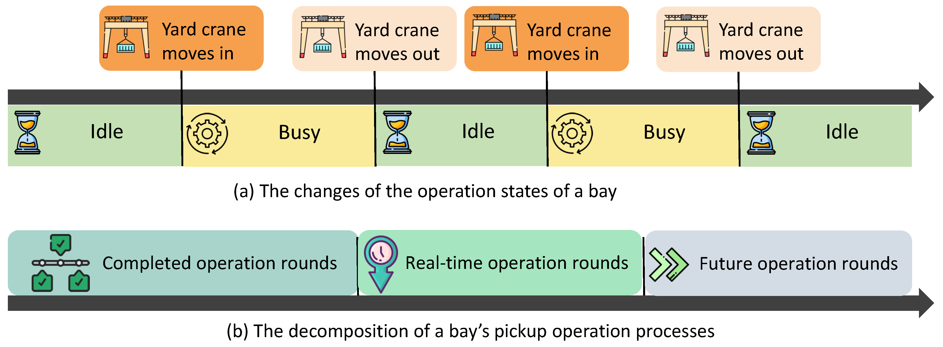
Figure 2.
An example of the LL rule. We set the priority of the target container to 0 and presented the decision process to relocate the blocking containers by LL. The container priority value marked by the red circle is the current blocking container. Numbers under the layout represent the minimum priority of each assignable stack and the increment of ENBC if moving the current blocking container into this stack. The blue number marks the optimal selection. The tag “” represents the container placed in the first stack and 3rd tier. The tag “” denotes an instruction, meaning the container “(1,3)” will be moved from the first stack into the fourth one.
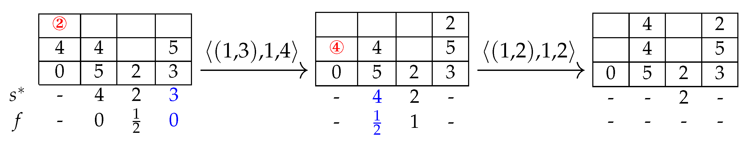
Figure 3.
An example of the MSS rule. We set the priority of the target container to 0 and presented the decision process to relocate the blocking containers by LL and MSS. The container priority value marked by the red circle is the current blocking container, and the container priority value marked by the orange circle is the relocating-ahead container. Numbers under the layout represent the minimum priority of each assignable stack and the increment of ENBC if moving the blocking container into this stack. The blue number marks the optimal selection.
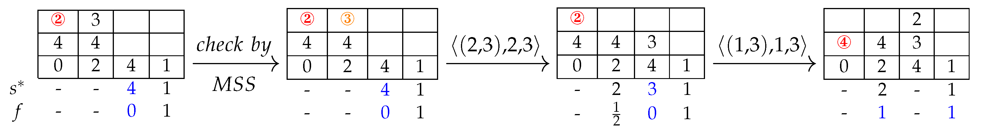
Figure 4.
An example of the FSS rule. The priorities of the target containers are set to 0. The container priority value marked by the red circle is the current blocking container, which does not have sequential placements to be reallocated. The blue downward arrows mark two containers that can be freed up for sequential placements, and the one whose stack minimum priority value (except for the topmost container) is closest to the current blocking container is selected.
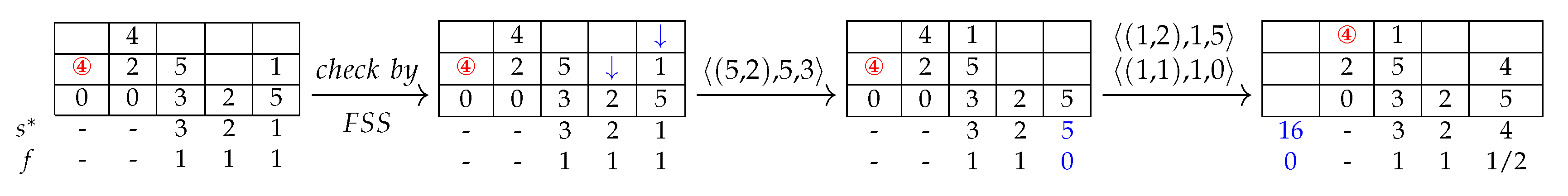
Figure 5.
Comparison between and at fill rate 50% and 67% respectively
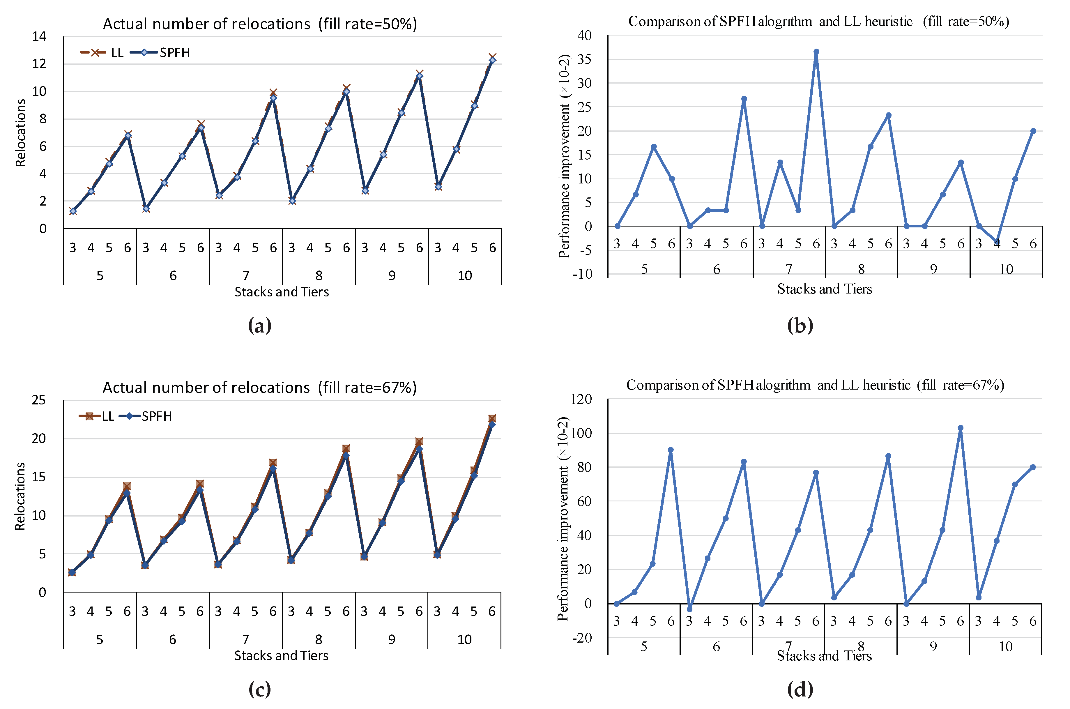

Table 1.
Runtime and completed instances of the heuristic with small batch instances.
| FillRate | 50 percent | 67 percent | |||||||||
| S | T | 3 | 4 | 5 | 6 | 3 | 4 | 5 | 6 | ||
| 5 | C | 8 | 10 | 13 | 15 | 10 | 14 | 17 | 20 | ||
| Solved | 30/30 | 30/30 | 30/30 | 30/30 | 30/30 | 30/30 | 30/30 | 30/30 | |||
| Time(s) | 0.043 | 0.005 | 0.008 | 0.011 | 0.134 | 0.008 | 0.011 | 0.011 | |||
| 6 | C | 9 | 12 | 15 | 18 | 12 | 16 | 20 | 24 | ||
| Solved | 30/30 | 30/30 | 30/30 | 30/30 | 30/30 | 30/30 | 30/30 | 30/30 | |||
| Time(s) | 0.009 | 0.006 | 0.012 | 0.013 | 0.011 | 0.010 | 0.013 | 0.015 | |||
| 7 | C | 12 | 14 | 18 | 21 | 14 | 19 | 24 | 28 | ||
| Solved | 30/30 | 30/30 | 30/30 | 30/30 | 30/30 | 30/30 | 30/30 | 30/30 | |||
| Time(s) | 0.006 | 0.011 | 0.011 | 0.013 | 0.011 | 0.014 | 0.013 | 0.021 | |||
| 8 | C | 12 | 16 | 20 | 24 | 16 | 21 | 27 | 32 | ||
| Solved | 30/30 | 30/30 | 30/30 | 30/30 | 30/30 | 30/30 | 30/30 | 30/30 | |||
| Time(s) | 0.008 | 0.010 | 0.012 | 0.019 | 0.007 | 0.011 | 0.014 | 0.027 | |||
| 9 | C | 14 | 18 | 23 | 27 | 18 | 24 | 30 | 36 | ||
| Solved | 30/30 | 30/30 | 30/30 | 30/30 | 30/30 | 30/30 | 30/30 | 30/30 | |||
| Time(s) | 0.008 | 0.009 | 0.013 | 0.014 | 0.011 | 0.013 | 0.020 | 0.026 | |||
| 10 | C | 15 | 20 | 25 | 30 | 20 | 27 | 34 | 40 | ||
| Solved | 30/30 | 30/30 | 30/30 | 30/30 | 30/30 | 30/30 | 30/30 | 30/30 | |||
| Time(s) | 0.007 | 0.012 | 0.015 | 0.014 | 0.012 | 0.013 | 0.019 | 0.024 | |||
Table 2.
Runtime and completed instances of the algorithm with small-batch instances.
| FillRate | 50 percent | 67 percent | |||||||||
| S | T | 3 | 4 | 5 | 6 | 3 | 4 | 5 | 6 | ||
| 5 | C | 8 | 10 | 13 | 15 | 10 | 14 | 17 | 20 | ||
| Solved | 30/30 | 30/30 | 30/30 | 30/30 | 30/30 | 30/30 | 30/30 | 30/30 | |||
| Time(s) | 0.022 | 0.021 | 0.014 | 0.021 | 0.038 | 0.016 | 0.027 | 0.023 | |||
| 6 | C | 9 | 12 | 15 | 18 | 12 | 16 | 20 | 24 | ||
| Solved | 30/30 | 30/30 | 30/30 | 30/30 | 30/30 | 30/30 | 30/30 | 30/30 | |||
| Time(s) | 0.013 | 0.012 | 0.022 | 0.016 | 0.014 | 0.020 | 0.021 | 0.030 | |||
| 7 | C | 12 | 14 | 18 | 21 | 14 | 19 | 24 | 28 | ||
| Solved | 30/30 | 30/30 | 30/30 | 30/30 | 30/30 | 30/30 | 30/30 | 30/30 | |||
| Time(s) | 0.016 | 0.016 | 0.011 | 0.015 | 0.020 | 0.026 | 0.021 | 0.027 | |||
| 8 | C | 12 | 16 | 20 | 24 | 16 | 21 | 27 | 32 | ||
| Solved | 30/30 | 30/30 | 30/30 | 30/30 | 30/30 | 30/30 | 30/30 | 30/30 | |||
| Time(s) | 0.013 | 0.014 | 0.013 | 0.024 | 0.014 | 0.018 | 0.021 | 0.029 | |||
| 9 | C | 14 | 18 | 23 | 27 | 18 | 24 | 30 | 36 | ||
| Solved | 30/30 | 30/30 | 30/30 | 30/30 | 30/30 | 30/30 | 30/30 | 30/30 | |||
| Time(s) | 0.012 | 0.014 | 0.018 | 0.015 | 0.012 | 0.021 | 0.033 | 0.038 | |||
| 10 | C | 15 | 20 | 25 | 30 | 20 | 27 | 34 | 40 | ||
| Solved | 30/30 | 30/30 | 30/30 | 30/30 | 30/30 | 30/30 | 30/30 | 30/30 | |||
| Time(s) | 0.008 | 0.021 | 0.019 | 0.023 | 0.0131 | 0.021 | 0.028 | 0.037 | |||
Table 3.
The results of the heuristic and the algorithm under 50% fill rate.
| Algorithm | LL | SPFH | ||||||||||||||
| S | T | IB | Max | Min | Stdev | Ieb | Max | Min | Stdev | Ieb | Max | Min | Stdev | |||
| 5 | 3 | 1.61 | 3.00 | 0.50 | 0.70 | 0.00 | 0.00 | 0.00 | 0.00 | 0.03 | 1.00 | 0.00 | 0.18 | |||
| 4 | 2.83 | 5.00 | 0.50 | 1.22 | 0.08 | 1.00 | 0.00 | 0.26 | 0.05 | 1.00 | 0.00 | 0.20 | ||||
| 5 | 4.48 | 5.50 | 2.50 | 0.93 | 0.33 | 1.50 | 0.00 | 0.47 | 0.57 | 2.50 | 0.00 | 0.64 | ||||
| 6 | 6.11 | 10.00 | 3.00 | 1.68 | 0.83 | 4.00 | 0.00 | 0.92 | 1.28 | 5.00 | 0.00 | 1.17 | ||||
| 6 | 3 | 1.63 | 3.50 | 0.00 | 0.94 | 0.02 | 0.50 | 0.00 | 0.09 | 0.08 | 1.00 | 0.00 | 0.26 | |||
| 4 | 3.49 | 6.00 | 1.00 | 1.29 | 0.03 | 1.00 | 0.00 | 0.18 | 0.23 | 2.00 | 0.00 | 0.50 | ||||
| 5 | 5.31 | 8.00 | 2.00 | 1.32 | 0.22 | 1.50 | 0.00 | 0.46 | 0.48 | 2.00 | 0.00 | 0.58 | ||||
| 6 | 7.05 | 10.50 | 4.00 | 1.55 | 0.70 | 4.00 | 0.00 | 0.86 | 1.05 | 3.00 | 0.00 | 1.00 | ||||
| 7 | 3 | 2.75 | 4.00 | 0.50 | 0.96 | 0.00 | 0.00 | 0.00 | 0.00 | 0.03 | 1.00 | 0.00 | 0.18 | |||
| 4 | 3.93 | 5.00 | 2.00 | 0.76 | 0.10 | 1.00 | 0.00 | 0.30 | 0.20 | 1.00 | 0.00 | 0.40 | ||||
| 5 | 6.42 | 9.50 | 3.00 | 1.39 | 0.22 | 1.00 | 0.00 | 0.33 | 0.60 | 3.00 | 0.00 | 0.81 | ||||
| 6 | 8.77 | 12.00 | 5.50 | 1.57 | 0.88 | 3.00 | 0.00 | 1.06 | 1.27 | 5.00 | 0.00 | 1.27 | ||||
| 8 | 3 | 2.22 | 4.00 | 0.00 | 1.17 | 0.00 | 0.00 | 0.00 | 0.00 | 0.10 | 1.00 | 0.00 | 0.30 | |||
| 4 | 4.68 | 8.00 | 1.50 | 1.62 | 0.06 | 1.00 | 0.00 | 0.21 | 0.26 | 1.00 | 0.00 | 0.43 | ||||
| 5 | 7.18 | 10.50 | 3.50 | 1.71 | 0.32 | 2.00 | 0.00 | 0.63 | 0.93 | 3.50 | 0.00 | 0.96 | ||||
| 6 | 9.45 | 13.00 | 4.50 | 1.85 | 0.87 | 4.00 | 0.00 | 1.19 | 1.32 | 5.00 | 0.00 | 1.27 | ||||
| 9 | 3 | 2.93 | 5.00 | 1.00 | 1.05 | 0.00 | 0.00 | 0.00 | 0.00 | 0.10 | 1.00 | 0.00 | 0.30 | |||
| 4 | 5.58 | 7.50 | 3.00 | 1.07 | 0.00 | 0.00 | 0.00 | 0.00 | 0.23 | 2.00 | 0.00 | 0.50 | ||||
| 5 | 8.55 | 13.00 | 5.00 | 2.13 | 0.20 | 2.00 | 0.00 | 0.46 | 0.67 | 2.00 | 0.00 | 0.65 | ||||
| 6 | 10.40 | 14.00 | 6.00 | 2.00 | 0.67 | 3.00 | 0.00 | 0.97 | 1.69 | 4.00 | 0.00 | 1.12 | ||||
| 10 | 3 | 3.18 | 6.00 | 1.00 | 1.35 | 0.00 | 0.00 | 0.00 | 0.00 | 0.20 | 2.00 | 0.00 | 0.48 | |||
| 4 | 6.15 | 9.00 | 3.00 | 1.25 | 0.03 | 0.50 | 0.00 | 0.12 | 0.35 | 2.00 | 0.00 | 0.59 | ||||
| 5 | 9.07 | 13.00 | 5.50 | 1.54 | 0.13 | 1.00 | 0.00 | 0.31 | 1.07 | 3.00 | 0.00 | 0.94 | ||||
| 6 | 11.90 | 16.50 | 5.50 | 2.40 | 0.57 | 3.50 | 0.00 | 0.88 | 1.43 | 3.00 | 0.00 | 0.85 | ||||
Table 4.
The results of the heuristic and the algorithm under 67% fill rate.
| Algorithm | LL | SPFH | ||||||||||||||
| S | T | IB | Max | Min | Stdev | Ieb | Max | Min | Stdev | Ieb | Max | Min | Stdev | |||
| 5 | 3 | 2.70 | 4.50 | 1.00 | 0.86 | 0.02 | 0.50 | 0.00 | 0.09 | 0.18 | 1.00 | 0.00 | 0.38 | |||
| 4 | 4.59 | 7.00 | 2.00 | 1.20 | 0.47 | 4.00 | 0.00 | 0.85 | 0.67 | 3.50 | 0.00 | 0.89 | ||||
| 5 | 7.50 | 11.00 | 4.00 | 1.60 | 1.21 | 4.00 | 0.00 | 0.98 | 1.71 | 5.00 | 0.00 | 0.98 | ||||
| 6 | 9.62 | 13.50 | 6.17 | 1.68 | 3.17 | 6.50 | 0.00 | 1.76 | 3.43 | 7.50 | 0.50 | 1.62 | ||||
| 6 | 3 | 3.55 | 6.00 | 0.50 | 1.18 | 0.08 | 1.00 | 0.00 | 0.26 | 0.28 | 1.00 | 0.00 | 0.44 | |||
| 4 | 6.13 | 9.00 | 3.00 | 1.48 | 0.52 | 2.00 | 0.00 | 0.65 | 0.90 | 3.00 | 0.00 | 0.82 | ||||
| 5 | 8.22 | 11.50 | 5.00 | 1.56 | 1.25 | 5.00 | 0.00 | 1.29 | 1.63 | 7.00 | 0.00 | 1.41 | ||||
| 6 | 11.57 | 15.00 | 7.50 | 1.78 | 2.42 | 6.00 | 0.00 | 1.61 | 2.92 | 8.00 | 0.00 | 2.00 | ||||
| 7 | 3 | 3.83 | 7.00 | 1.00 | 1.24 | 0.07 | 1.00 | 0.00 | 0.21 | 0.17 | 1.00 | 0.00 | 0.35 | |||
| 4 | 6.20 | 9.00 | 2.00 | 1.70 | 0.57 | 2.00 | 0.00 | 0.70 | 0.80 | 4.00 | 0.00 | 1.00 | ||||
| 5 | 9.68 | 12.50 | 6.00 | 1.58 | 1.31 | 4.00 | 0.00 | 1.11 | 1.81 | 4.00 | 0.00 | 1.11 | ||||
| 6 | 13.42 | 17.00 | 8.50 | 1.92 | 2.35 | 5.50 | 0.00 | 1.36 | 3.00 | 6.50 | 0.00 | 1.40 | ||||
| 8 | 3 | 4.41 | 7.00 | 1.00 | 1.53 | 0.07 | 1.00 | 0.00 | 0.25 | 0.33 | 2.00 | 0.00 | 0.54 | |||
| 4 | 7.60 | 11.50 | 4.00 | 1.85 | 0.37 | 4.00 | 0.00 | 0.81 | 0.75 | 3.00 | 0.00 | 0.87 | ||||
| 5 | 11.54 | 15.00 | 6.50 | 1.67 | 1.13 | 4.00 | 0.00 | 1.10 | 2.23 | 5.00 | 0.00 | 1.26 | ||||
| 6 | 15.57 | 20.50 | 11.50 | 2.49 | 2.38 | 7.50 | 0.00 | 1.83 | 3.28 | 9.50 | 0.00 | 2.05 | ||||
| 9 | 3 | 4.79 | 8.00 | 1.50 | 1.43 | 0.08 | 1.00 | 0.00 | 0.26 | 0.35 | 1.00 | 0.00 | 0.47 | |||
| 4 | 8.98 | 13.00 | 6.00 | 1.72 | 0.35 | 2.00 | 0.00 | 0.55 | 1.10 | 4.00 | 0.00 | 1.03 | ||||
| 5 | 13.11 | 17.00 | 8.67 | 1.79 | 1.35 | 4.00 | 0.00 | 1.30 | 2.20 | 5.00 | 0.00 | 1.35 | ||||
| 6 | 16.67 | 20.50 | 12.17 | 1.98 | 2.83 | 7.50 | 0.00 | 2.27 | 3.80 | 8.50 | 0.00 | 1.91 | ||||
| 10 | 3 | 5.21 | 8.17 | 2.00 | 1.31 | 0.08 | 1.00 | 0.00 | 0.26 | 0.32 | 2.00 | 0.00 | 0.52 | |||
| 4 | 9.18 | 13.00 | 5.50 | 2.06 | 0.67 | 4.67 | 0.00 | 1.02 | 1.05 | 3.00 | 0.00 | 0.93 | ||||
| 5 | 14.44 | 19.50 | 8.50 | 2.43 | 1.28 | 6.00 | 0.00 | 1.37 | 1.95 | 6.00 | 0.00 | 1.41 | ||||
| 6 | 19.52 | 23.50 | 14.00 | 2.39 | 2.48 | 7.00 | 0.00 | 1.90 | 3.73 | 9.00 | 0.00 | 2.07 | ||||
Table 5.
The optimization objective of the heuristic and algorithm .
| Fill Rate | 50% | 67% | |||||||||||||||||||
| Algorithms | LL | SPFH | LL | SPFH | |||||||||||||||||
| S | T | IB | Ieb | Act | G | Ieb | Act | G | IB | Ieb | Act | G | Ieb | Act | G | ||||||
| 5 | 3 | 1.61 | 0.00 | 1.27 | 21.33% | 0.03 | 1.27 | 22.92% | 2.70 | 0.02 | 2.63 | 3.07% | 0.18 | 2.63 | 8.67% | ||||||
| 4 | 2.83 | 0.08 | 2.77 | 5.03% | 0.05 | 2.70 | 6.25% | 4.59 | 0.47 | 4.93 | 2.52% | 0.67 | 4.87 | 7.50% | |||||||
| 5 | 4.48 | 0.33 | 4.90 | -1.81% | 0.57 | 4.73 | 6.21% | 7.50 | 1.21 | 9.57 | -9.89% | 1.71 | 9.33 | -1.39% | |||||||
| 6 | 6.11 | 0.83 | 6.90 | 0.55% | 1.28 | 6.80 | 7.96% | 9.62 | 3.17 | 13.83 | -8.17% | 3.43 | 12.93 | 0.94% | |||||||
| 6 | 3 | 1.63 | 0.02 | 1.43 | 12.96% | 0.08 | 1.43 | 16.34% | 3.55 | 0.08 | 3.47 | 4.59% | 0.28 | 3.50 | 8.70% | ||||||
| 4 | 3.49 | 0.03 | 3.37 | 4.45% | 0.23 | 3.33 | 10.47% | 6.13 | 0.52 | 6.90 | -3.76% | 0.90 | 6.63 | 5.69% | |||||||
| 5 | 5.31 | 0.22 | 5.30 | 4.11% | 0.48 | 5.27 | 9.09% | 8.22 | 1.25 | 9.70 | -2.46% | 1.63 | 9.20 | 6.60% | |||||||
| 6 | 7.05 | 0.70 | 7.63 | 1.51% | 1.05 | 7.37 | 9.05% | 11.57 | 2.42 | 14.17 | -1.31% | 2.92 | 13.33 | 7.94% | |||||||
| 7 | 3 | 2.75 | 0.00 | 2.43 | 11.52% | 0.03 | 2.43 | 12.57% | 3.83 | 0.07 | 3.60 | 7.69% | 0.17 | 3.60 | 10.00% | ||||||
| 4 | 3.93 | 0.10 | 3.87 | 4.05% | 0.20 | 3.73 | 9.60% | 6.20 | 0.57 | 6.77 | 0.00% | 0.80 | 6.60 | 5.71% | |||||||
| 5 | 6.42 | 0.22 | 6.40 | 3.57% | 0.60 | 6.37 | 9.31% | 9.68 | 1.31 | 11.17 | -1.62% | 1.81 | 10.73 | 6.58% | |||||||
| 6 | 8.77 | 0.88 | 9.90 | -2.56% | 1.27 | 9.53 | 5.07% | 13.42 | 2.35 | 16.87 | -6.98% | 3.00 | 16.10 | 1.93% | |||||||
| 8 | 3 | 2.22 | 0.00 | 2.03 | 8.41% | 0.10 | 2.03 | 12.36% | 4.41 | 0.07 | 4.20 | 6.09% | 0.33 | 4.17 | 12.08% | ||||||
| 4 | 4.68 | 0.06 | 4.40 | 7.09% | 0.26 | 4.37 | 11.53% | 7.60 | 0.37 | 7.83 | 1.67% | 0.75 | 7.67 | 8.18% | |||||||
| 5 | 7.18 | 0.32 | 7.47 | 0.40% | 0.93 | 7.30 | 10.02% | 11.54 | 1.13 | 12.90 | -1.80% | 2.23 | 12.47 | 9.48% | |||||||
| 6 | 9.45 | 0.87 | 10.23 | 0.81% | 1.32 | 10.00 | 7.12% | 15.57 | 2.38 | 18.70 | -4.18% | 3.28 | 17.83 | 5.39% | |||||||
| 9 | 3 | 2.93 | 0.00 | 2.77 | 5.57% | 0.10 | 2.77 | 8.69% | 4.79 | 0.08 | 4.60 | 5.69% | 0.35 | 4.60 | 10.58% | ||||||
| 4 | 5.58 | 0.00 | 5.40 | 3.23% | 0.23 | 5.40 | 7.11% | 8.98 | 0.35 | 9.13 | 2.14% | 1.10 | 9.00 | 10.74% | |||||||
| 5 | 8.55 | 0.20 | 8.50 | 2.86% | 0.67 | 8.43 | 8.50% | 13.11 | 1.35 | 14.90 | -3.07% | 2.20 | 14.47 | 5.48% | |||||||
| 6 | 10.40 | 0.67 | 11.27 | -1.76% | 1.69 | 11.13 | 7.90% | 16.67 | 2.83 | 19.63 | -0.66% | 3.80 | 18.60 | 9.15% | |||||||
| 10 | 3 | 3.18 | 0.00 | 3.03 | 4.61% | 0.20 | 3.03 | 10.26% | 5.21 | 0.08 | 4.90 | 7.35% | 0.32 | 4.87 | 11.87% | ||||||
| 4 | 6.15 | 0.03 | 5.77 | 6.74% | 0.35 | 5.80 | 10.77% | 9.18 | 0.67 | 9.90 | -0.45% | 1.05 | 9.53 | 6.84% | |||||||
| 5 | 9.07 | 0.13 | 9.07 | 1.48% | 1.07 | 8.97 | 11.54% | 14.44 | 1.28 | 15.87 | -0.92% | 1.95 | 15.17 | 7.46% | |||||||
| 6 | 11.90 | 0.57 | 12.47 | 0.00% | 1.43 | 12.27 | 8.00% | 19.52 | 2.48 | 22.60 | -2.73% | 3.73 | 21.80 | 6.24% | |||||||
Table 6.
Validation of the heuristic and algorithm with large instances in the real-time operation scenario of SCRP.
Table 6.
Validation of the heuristic and algorithm with large instances in the real-time operation scenario of SCRP.
| LL | SPFH | ||||||||||||||||
| S | T | W | B | FillRate | I | IB | MT | AT | Act | MT | AT | Act | |||||
| 10 | 8 | 8 | 5 | 0.500 | 30/30 | 18.23 | 0.35 | 0.03 | 3.11 | 26.99 | 0.18 | 0.04 | 4.50 | 27.27 | |||
| 6 | 0.600 | 30/30 | 23.43 | 0.56 | 0.06 | 6.75 | 33.49 | 1.16 | 0.10 | 7.34 | 34.94 | ||||||
| 7 | 0.700 | 30/30 | 29.67 | 4.98 | 0.32 | 12.71 | 46.41 | 8.26 | 0.50 | 12.97 | 46.21 | ||||||
| 8 | 0.800 | 30/30 | 36.70 | 34.97 | 2.57 | 20.74 | 61.32 | 49.47 | 3.89 | 22.36 | 62.50 | ||||||
| 10 | 4 | 0.500 | 30/30 | 17.73 | 0.05 | 0.01 | 3.68 | 25.27 | 0.10 | 0.02 | 4.75 | 27.74 | |||||
| 5 | 0.625 | 30/30 | 25.80 | 0.19 | 0.04 | 6.73 | 37.65 | 0.34 | 0.06 | 8.04 | 38.17 | ||||||
| 6 | 0.750 | 30/30 | 32.47 | 0.56 | 0.09 | 14.57 | 51.65 | 0.96 | 0.13 | 14.99 | 52.72 | ||||||
| 7 | 0.875 | 30/30 | 41.77 | 6.21 | 0.60 | 23.93 | 71.10 | 11.46 | 1.33 | 25.51 | 71.10 | ||||||
| 9 | 8 | 6 | 0.533 | 30/30 | 22.83 | 0.74 | 0.07 | 6.48 | 34.24 | 1.26 | 0.11 | 7.71 | 35.85 | ||||
| 7 | 0.622 | 30/30 | 29.67 | 1.68 | 0.17 | 10.67 | 46.10 | 2.82 | 0.29 | 11.69 | 45.92 | ||||||
| 8 | 0.711 | 30/30 | 36.30 | 7.09 | 0.61 | 19.35 | 59.31 | 12.09 | 0.98 | 19.19 | 59.18 | ||||||
| 9 | 0.800 | 30/30 | 41.13 | 40.47 | 5.01 | 31.87 | 77.04 | 58.68 | 8.74 | 35.40 | 80.77 | ||||||
| 10 | 5 | 0.556 | 30/30 | 25.53 | 0.11 | 0.03 | 7.13 | 36.94 | 0.17 | 0.04 | 8.63 | 37.83 | |||||
| 6 | 0.667 | 30/30 | 33.37 | 1.26 | 0.12 | 12.99 | 51.84 | 2.14 | 0.20 | 14.59 | 52.15 | ||||||
| 7 | 0.778 | 30/30 | 42.40 | 5.80 | 0.54 | 24.09 | 71.75 | 10.07 | 0.89 | 25.03 | 72.97 | ||||||
| 12 | 10 | 8 | 8 | 0.533 | 30/30 | 33.97 | 1.44 | 0.27 | 9.45 | 46.70 | 2.55 | 0.43 | 10.19 | 49.95 | |||
| 9 | 0.600 | 30/30 | 39.00 | 2358.47 | 84.57 | 19.60 | 62.58 | 94.83 | 9.97 | 23.41 | 66.14 | ||||||
| 10 | 0.667 | 30/30 | 45.07 | 93.00 | 16.98 | 38.05 | 88.81 | 167.34 | 26.58 | 46.43 | 95.01 | ||||||
| 11 | 0.733 | 12/30 | 50.94 | 7377.33 | 478.17 | 48.99 | 103.61 | 4010.35 | 373.49 | 59.00 | 113.84 | ||||||
| 12 | 0.800 | 0/30 | 0.00 | 0.00 | 0.00 | 0.00 | - | 0.00 | 0.00 | 0.00 | 5.72 | ||||||
| 10 | 8 | 0.667 | 30/30 | 49.61 | 68.87 | 3.79 | 24.44 | 78.34 | 111.87 | 6.33 | 27.21 | 81.81 | |||||
| 9 | 0.750 | 30/30 | 57.92 | 69.71 | 3.95 | 33.42 | 96.96 | 113.61 | 6.39 | 35.35 | 99.00 | ||||||
| 10 | 0.833 | 30/30 | 67.15 | 4115.17 | 628.84 | 66.94 | 138.10 | 3925.53 | 567.58 | 60.74 | 133.42 | ||||||
| 11 | 0.917 | 20/30 | 72.14 | 4818.37 | 841.89 | 99.55 | 176.27 | 3925.53 | 888.10 | 90.04 | 166.60 |
Disclaimer/Publisher’s Note: The statements, opinions and data contained in all publications are solely those of the individual author(s) and contributor(s) and not of MDPI and/or the editor(s). MDPI and/or the editor(s) disclaim responsibility for any injury to people or property resulting from any ideas, methods, instructions or products referred to in the content. |
© 2024 by the authors. Licensee MDPI, Basel, Switzerland. This article is an open access article distributed under the terms and conditions of the Creative Commons Attribution (CC BY) license (http://creativecommons.org/licenses/by/4.0/).
Copyright: This open access article is published under a Creative Commons CC BY 4.0 license, which permit the free download, distribution, and reuse, provided that the author and preprint are cited in any reuse.


