Submitted:
02 January 2024
Posted:
03 January 2024
You are already at the latest version
Abstract
Bosons are particles that can occupy the same quantum state. Identical classical particles are considered distinguishable, but with bosons this is no longer the case. With bosons 1 and 2 in states α and β, the compound state function, ΨS=(1/2)Ψα(1)Ψβ(2)+Ψβ(1)Ψα(2), does not change when the particles are interchanged, i.e., there is one state where classically there would be two. This leads to boson statistics, which is different from Boltzmann statistics in that it favors putting more particles in the same state. For a sufficiently low temperature, it is possible that all bosons aggregate in the ground state where they effectively form a single megaparticle. We cover boson statistics and show how and why Bose-Einstein condensation can occur. We also show how growing networks like the WWW, the economy, or citation networks in scientific literature can follow boson statistics. Analyses of Bose-Einstein condensation have generally assumed a bath with a temperature, i.e., a thermal equilibrium where random collisions lead to a Gaussian-noise-term. However, many setups in physics involve conversion or transport of energy, i.e., nonequilibrium. Nonequilibrium noise is commonly characterized by the frequent occurrence of large kicks, i.e., outliers. We model this by implementing α-stable noise. No temperature exists in that case. We find that Bose-Einstein condensation is still theoretically possible, but probably much harder to engineer. Social and economic traffic is also often best modeled as nonequilibrium and our results may be significant in these contexts.
Keywords:
Bosons
; Bose-Einstein Condensation
; Bianconi-Barabási Model
; growing networks
; Lévy Noise
; Nonequilibrium
1. Introduction
The aggregation discussed in this Special Issue is mostly chemical in nature. Understanding such aggregation is relevant throughout the applied sciences. One of the reasons that sedimentation occurs in a river delta is that the medium for suspended particles becomes more salty upon approaching the ocean. The sodium and chloride ions then screen away the repulsive interaction between the suspended particles. Aggregation occurs and the newly formed large clusters sink to the bottom [1,2]. Many biological phenomena involve aggregation too. Bone development and teeth development, but also gout, kidney stones and gallstones, happen as a result of aggregation. Neurodegenerative diseases, like Alzheimer, are associated with the aggregation of misfolded proteins [3]. The understanding of aggregation in a living cell is often complicated as the diffusion of small molecules is not free, but commonly hindered and anomalous [4]. However, also with anomalous diffusion, the actual aggregation is the outcome of a “competition” between the drive to maximize entropy through diffusion and the drive to minimize energy through binding.
For most of the aggregation that is significant in real life and for all of the examples in the previous paragraph, the medium is water. It often happens that observed phenomena defy easy explanation. It is then tempting to invoke quantum mechanics to solve the puzzle [5]. However, it must be realized that quantum coherent domains, i.e. domains within the liquid that can be described by a single quantum mechanical state function, can not develop and survive in liquid water. At room temperature, water molecules move with a speed of several hundred meters per second. A water molecule then collides about a trillion (1012) times per second with another molecule and the mean free path is about the size of the molecule itself. With that many Brownian collisions, no possible domain can stay isolated for more than a picosecond [6,7]. Biological functioning should ensue from physical chemistry. “Quantumbiology” is a misapprehension.
To see aggregation in a regime where quantum mechanics is at the helm, we have to go to extremely low temperatures. In 1995 a group in Boulder, Colorado, succeeded in cooling a cluster of a few thousand rubidium atoms down to below 170 nanokelvin [8]. They thus created a Bose-Einstein condensate, i.e., a significant fraction of particles was in the quantum mechanical ground state and effectively behaved as one megaparticle. As the cosmic background radiation that fills the universe corresponds to a temperature of 2.7 K, the Bose-Einstein condensate that was produced in Boulder may well be the first atomic-gaseous-matter one to have ever happened in the history of the entire universe. The possibility of a Bose-Einstein condensate was theoretically predicted in 1925 by Albert Einstein and Satyendra Nath Bose. Subsequently, Bose-Einstein condensation was invoked as an explanation for superfluidity. A laser can be thought of as a Bose-Einstein condensate with photons as the constituent “material.” The 1995 achievement was awarded with a Nobel Prize in 2001. At present, many groups are creating Bose-Einstein condensates and researching their properties.
The particles that Bose and Einstein theorized about are bosons [9]. These are particles that are allowed to occupy the same quantum state. Unlike classical particles they are indistinguishable, i.e., they can’t be marked and followed individually. In Section 2 it will be explained how boson statistics is fundamentally different from the Boltzmann statistics that rules the world of chemistry. In ordinary chemical kinetics, molecules move independently from one state to another. In Bose-Einstein statistics particles appear more likely to occupy an already occupied state. In a Bose-Einstein condensate the lowest energy level effectively “sucks in” all the bosons and the formation of a Bose-Einstein condensate is a true phase transition. At that phase transition the bosons’ drive to aggregate into one quantum mechanical state triumphs over Brownian motion and its elementary “quantum” of . In Section 2 we will derive equations that are associated with the phase transition.
Every publishing scientist knows that a paper that is already cited a lot is also paper that has a bigger chance of getting more citations. Likewise, a plumber that already has a lot of customers is the one that acquires more customers and a website that is linked a lot will most rapidly accumulate more links [10]. This is mindful of boson statistics and, indeed, growing networks that ensue from a flow of information exhibit Bose-Einstein statistics. The analogy is elaborated on in Section 3.
Nonequilibrium systems commonly exhibit Lévy noise [11]. This means that the distribution for the magnitude of the Brownian fluctuations has a “fat” power-law tail. Large Brownian kicks are then more common as compared to the ordinary Gaussian distribution. Lévy noise thus accounts for the “outliers” that frequently occur away from equilibrium. In Section 4 we consider a two-state system, i.e., a potential with two wells and a barrier in between. The bosons in the two-state system are subjected to Lévy noise. The barrier is sufficiently high for a barrier crossing to be a rare event. We next derive the distribution of the bosons over the two wells. It is found that the formation of a Bose-Einstein condensate is still possible when the noise is Lévy.
In Section 5 we reflect on the meaning of the result. We discuss the issues involved in relating our final formulae to actual experiments with bosons or to real-life growing networks.
2. The Chemical Kinetics Of Bosons
Legend has it that the intellectual genesis of the Bose-Einstein condensate occurred when Satyendra Nath Bose made an elementary mistake as he was assessing coin tosses. He told his class that when tossing two fair coins, the three possible outcomes (HH, HT, TT, where H = head and T= tail) each have the same probability of 1/3. A middle schooler could have pointed out that there are two ways to get one head and one tail (HT and TH) and that ultimately for both HH and TT there is a chance of 1/4, and that for one H and one T the chance is 1/2.
The “1/3, 1/3, 1/3"-assessment, however, would have been correct at an atomic level if the objects of interest are no longer macroscopic coins or other classical particles, but identical, “bose" particles subject to the rules of Quantum Mechanics. “Bose particles" are more commonly called “bosons" and they can occupy the same quantum state. Imagine two indistinguishable bosons and two available states. The particles are like the coins of the previous paragraph and the states are like head vs. tail. With HT and TH being one and the same state, we get the ”1/3, 1/3, 1/3” distribution.
What the previous paragraph makes clear is that, with boson statistics, the states HH and TT get a higher probability as compared to classical particle statistics. In other words, bosons “like to be” in the same state. We will show below how this tendency gets even stronger if more particles are involved.
For two indistinguishable identical articles, 1 and 2, in states and , the state function should be the same when the articles are interchanged, i.e., the wave function should be symmetric. This forces us to adopt the following form:
Here is the state function that describes the two-boson system. The states and are orthogonal and the term has been entered to normalize . It guarantees that if and
.
Now imagine the two particles in the same state, i.e. . We then have and find for the probability density:
The prefactor “2” results from the fact that state functions add vectorially. This feature, combined with the symmetrization and the aforementioned normalization, has dramatic consequences. If we had not realized that the indistinguishability leads to the form Eq. (1) and stuck to a straightforward product of ’s, we would have not run into this factor. In the classical picture, particles behave independently. But for a boson, the probability for a particle to be in a certain state doubles if that state already has a particle in it!
With 3 particles sharing the same state, the prefactor in the probability density term, i.e. Eq. (2), is . For n particles, the prefactor equals .
Let represent the probability that a first boson goes into an initially empty state. If the aforementioned enhancement effects did not exist, then it would not matter how many particles are in the state and, with n particles, the probability that all n particles are in that state is simply . But with bosons, the enhancement leads to [9].
All in all, if a quantum state already has n bosons, then the probability for one more boson to enter that state is enhanced by a factor . That factor does not exist in the classical picture where all particles behave independently.
At this point it makes sense to briefly reconsider the Boltzmann statistics that we have for independent particles at finite temperature T. We will compare this to boson statistics. Suppose we have two states and transitions between them:
Here the transition rate from to is and the transition rate from to is . In the traditional Boltzmann picture, each particle behaves independently and, at equilibrium, we have for the numbers and in the states and [12]:
where represents the energy difference between the two states, i.e. , and represents Boltzmann’s constant. Note that at equilibrium we also have detailed balance:
i.e., there is as much traffic from to as there is from to .
For bosons the same equilibrium condition, i.e. Eq. (5), has to hold. However, as we just saw, with bosons the transition rate into a state goes up with the number of particles already in that state, i..e., and . Equation (5) then turns into
where and are the classical Boltzmann transition rates that follow . With , we then find for an equilibrium distribution involving bosons:
Equation (7) readily generalizes if there are more than two states. Identifying the term left and right of the equal sign in Eq. (7) with C, we find for the number of particles in any state j:
For a Boltzmann distribution, the expression “” turns out the same for every state j. So, ultimately, it is the “” in the denominator of Eq. (8) that makes the Bose-Einstein distribution different from the Boltzmann distribution.
A simple example will clarify how drastically different the Boltzmann distribution and the Bose-Einstein distribution nevertheless are. Imagine a two-state system with a ground state and an excited state. We take the ground-state energy to be zero and the excited-state energy to be . We let the energy be large compared to . We have a large number of particles that is distributed over the ground state and the excited state, i.e., . With the Boltzmann distribution we have . After some algebra and neglecting relative to “1”, we derive for the Boltzmann case
For the case of a Bose-Einstein distribution, we turn to Eq. (7) and write down:
With , the left-hand-side approaches one. That necessitates an that is much smaller than one. We thus find
Ultimately, will be smaller than 1 and this means that Eq. (11) merely gives the probability that, upon making an observation, a particle is found in the excited state.
Classical thermodynamics makes a distinction between intrinsic and extrinsic variables. Extensive variables are variables that scale proportionally with the amount of material in the system. Mass and entropy are examples of extensive variables. Intensive variables are those that do not depend on system size. Pressure and concentration are examples of intensive variables. With Eq. (9) and Eq. (11), we see that the occupation of the excited state, , is an extensive variable in case of a Boltzmann distribution, but that it can be an intensive variable if bosons are involved. It should be noted here that with bosons, the occupation of the excited state is an extensive variable if is small (cf. Eq. (7)). Next, the extensive-intensive transition is the actual Bose-Einstein condensation. In our two state example, it is not a phase transition at a fixed and finite temperature like in the Boulder experiment and its theoretical understanding. With the two-state system, the extensive-intensive transition occurs gradually as T is decreased.
For the actual 1995 Bose-Einstein condensate that was created in Boulder, the setup was more intricate than the two-state system (cf. Eq. (3)) that we looked at here. There, several thousand bosons were “trapped” in what is most easily modeled as an infinite square well [13] in 3D, i.e., a particle in a box with “walls” of infinite potential energy. Energy levels are sufficiently close together in this setup that they can be taken to form a continuum. It takes very low temperatures in that case to force all the bosons into the ground state. Upon working out the mathematics, a singularity appears at a small but nonzero critical temperature. That is where the phase transition happens [14].
The term “Bose-Einstein condensate” brings to mind the image of a liquid-vapor transition. But this is a poor analogy. The idea of distinct particles is to be abandoned as there are no individual motions or positions anymore in the Bose-Einstein condensate - state functions overlap and atoms have effectively merged. The state of the entire system is to be understood through quantum mechanics: as individual level state functions that are multiplied and next symmetrized as in Eq. (1).
Photons are bosons. As they all have the same wavelength and phase, the photons in a laser beam are in essence a Bose-Einstein condensate. Because it is in effect one particle in one quantum state, a laser beam is readily controlled and manipulated. Laser technology was first developed in the 1960s, but today has many applications. Likewise, there are technology prospects for atomic and molecular Bose-Einstein condensates once there is technology to produce them more cheaply and easily.
3. Bose-Einstein Condensation In Networks
The legendary businessman and investor Charles Munger once said in all seriousness “The way to get rich is to keep ten million dollars in your checking account for in case a good deal comes along.” For the vast majority of people this statement is not so much realistic investment guidance as that it is another affirmation of the folk wisdom that it takes money to make money. In the Gospel of Matthew (25:29) it says “For to everyone who has, more shall be given” and, because of this, “having to be rich to get rich” is also commonly known as the Matthew Effect.
The Matthew Effect is a positive feedback mechanism that does not just apply to the acquisition of money. Websurfers join a social networking site like FaceBook because other websurfers are already on it. Another example is constituted by the citation numbers that are central to a scientist’s prestige. Every working and publishing scientist knows that citations come more easily once you are already cited.
In a 1968 article in Science, Robert K. Merton describes how recognition in science goes to scientists that have already been recognized [15]. With the recognition, the working scientist also gets the funds and facilities that, in turn, help him or her to get even more recognition. Because of this feedback cycle, many achievements get overrated while other achievements go unrecognized. Merton’s article has no statistics or graphs. The backup for the claim is mostly anecdotal. But with the electronic databases and computing power of the 21st century, it is possible to put quantitative muscle behind the insights of the evangelist Matthew and the sociologist Merton.
Worldwide, more than 45,000 scientific journals publish more than 5 million scientific articles annually (see, e.g., https://wordsrated.com/number-of-academic-papers-published-per-year/). Scientific articles citing other scientific articles constitute a large and growing network. Through services like Google Scholar, PubMed, ResearchGate, Scopus, Web of Science, and CiteSeer, data on the network can be readily gathered.
With the newly available abundance of data, theory on networks was established concurrently and, in 2001, Bianconi and Barabási proposed a simple model for a growing network [16]. The Matthew Effect was part of their setup. Upon working out the model, they found that Bose-Einstein condensation can occur as parameters are varied. We will briefly discuss the model below.
We start with a single node “1”. Next nodes are added in sequence. With each added node, m links from the new node to previous nodes are also added. In Figure 1 we take . The probability that a new node connects to a node i in the existing network is
where is the number of links that node i has already gathered and is a “fitness parameter.” With different values for we can account for the fact that some websites are innately more inviting and likely to be linked to. In the case of scientific articles, it is through that we distinguish between well-written articles with interesting new results and inferior articles. Through we associate every with an energy . Here T plays the role of a temperature. It is obvious that the node with the highest value for the fitness corresponds to the ground state, i.e., the state with the lowest energy (cf. Figure 1).
The difference between the setup discussed in Section 2 and the growing networks is that in the latter case particles keep being added as time evolves. After having been added, particles remain forever at the same level that they were entered at. The asymptotic distribution is established as the thermodynamic limit, i.e. , is approached.
Reference [16] first considers what happens if all ’s are the same. It is derived that in that case the Matthew Effect does not overcome the stochasticity. Nodes and links are added at the same rate and it is found that the fraction of the total number of links that any particular node acquires goes to zero as .
But what if we have different values for ? Given a distribution for the ’s, we can space out the ensuing distribution of the ’s by taking a temperature that is closer to zero. There then appears to be a temperature at which a phase transition occurs. Below a finite fraction of all links will connect to the ground state as and the fraction will remain finite as the network keeps growing.
4. When Bosons In A Double Well Potential Are Subjected To L évy Noise
The Langevin Equation describes a trajectory of an overdamped particle when it is in a potential and subject to Brownian kicks:
Here motion is along the x-axis. The parameter represents the mobility of the particle in the medium. The mobility is the emergent ratio when a force F is applied and an average speed v through the medium results. The term describes the Brownian kicks, i.e., the thermal noise. Here D is the diffusion coefficient of the particle. For equilibrium systems, the noise is generally taken to be white and Gaussian [17]. The noise term is normalized through , where represents a Dirac delta function. At equilibrium there exists a relation that connects the noise strength and the mobility: . Here is Boltzmann’s constant and T is the absolute temperature. This is Einstein’s well-known Fluctuation Dissipation Theorem [17].
Equation (13) is easy to simulate. The “white”-ness of the noise means that there is no correlation between the value and the value one timestep later. The values for are ultimately independent and are drawn from a Gaussian distribution.
The “Gaussian” part of the equilibrium noise refers to the distribution of the kick-sizes. The Gaussian is the go-to distribution for many applications as the Central Limit Theorem tells us that the cumulative effect of multiple independent stochastic inputs converges to a Gaussian distribution [17]. In our case, the noise contribution to at the i-th timestep is the result of a large number of collisions during between the overdamped particle described by Eq. (13) and molecules from the medium. So Gaussianness for should be a valid assumption. However, an important condition here is that all these “stochastic inputs” have a finite variance. Only if that condition is satisfied, is the Gaussian distribution an “attractor.”
Over the last century, however, it has become increasingly clear that the noise in many nonequilibrium processes is characterized by large outliers. Plasma turbulence [18], financial market dynamics [19,20,21], and climate change studies [22] provide examples. Also in data from physiology [23] and solar physics [24,25], it appears that the noise contains more large jumps than can be accounted for with the standard Gaussian distribution.
To account for the nonequilibrium environment and the ensuing outliers, we commonly draw the values of , not from a Gaussian distribution, but from a so-called -stable distribution [11,26]. Such a distribution is also often called a Lévy-stable distribution.
The Gaussian distribution has an exponential tail, i.e., as , where denotes the standard deviation of the Gaussian. The rapid convergence to zero of the exponential tail means that the probability to make a big jump is very small and effectively negligible. For an -stable distribution, the asymptotic behavior is described by a power law:
Here is the so-called stability index for which we have . For the Gaussian is re-obtained. The power law converges slower than the exponential. A result of this is that outliers, i.e. large “Lévy jumps,” regularly occur. With the standard deviation , the Gaussian contains a characteristic kicksize. But the Lévy distribution features no characteristic kicksize and the root-mean-square of actually diverges.
Where a Gaussian distribution results for a process that is the cumulative effect of stochastic processes with a finite standard deviation, an -stable distribution results when infinite standard deviations come into play. The analytic expression for the -stable distribution is huge and cumbersome [27], but in Fourier space a concise formula ensues. For a symmetric, zero-centered -stable distribution, the generating function is:
Here c is a scale factor. For the -stable distribution is the simple and well-known Cauchy distribution, i.e. . With the commands “RandomVariate” and “StableDistribution,” the software package Mathematica readily generates a large set of -stable-distributed numbers and simulating Eq. (13) where the Gaussian noise (i.e. ) is replaced by Lévy noise (i.e. ) is a matter of a few lines of code.
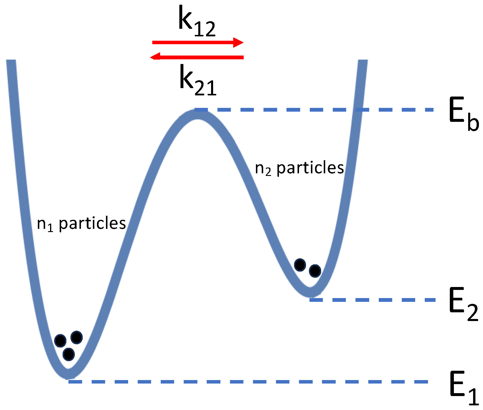
A two-state system (cf. Eq. (3)) is commonly depicted as a double well where the minima represent the states and and the maximum in between is an activation barrier that needs to be mounted if a particle transits from one state to the other. Figure 2 depicts such a double well. The horizontal coordinate can be thought of as a reaction coordinate along which the change-of-state progresses. The vertical coordinate is the energy. The double well as in Figure 2 is readily implemented as the in Eq. (13).
The transition rates and derive from the probability that a particle in one well (cf. Figure 2) receives enough energy from the noise to mount the barrier and move to the other well. With Gaussian noise the setup of Figure 2 leads to and , where C is a positive constant. These expressions imply Eq. (4). Onsager and Machlup showed in 1953 that, with Gaussian noise, the most likely trajectory to lead to a barrier crossing involves a kind of “Brownian conspiracy” in which a number of subsequent kicks are all in the same direction and of roughly the same magnitude [28,29,30].
Also when the particles in the double well are subjected to Lévy noise, there will ultimately be a steady state distribution (cf. Eq. (5)) of the particles over the two wells. However, with Lévy noise the most likely barrier-crossing trajectory is not a “lucky” sequence of kicks, but one large kick from the power-law-tail of the distribution of kicksizes [31,32]. When the mobility is sufficiently large, the energy necessary to overcome friction becomes negligible relative to the energy necessary to mount the barrier. This leads to and , where is again a positive constant. For the steady state distribution we then obtain:
This formula was derived in Ref. [33] and details about the derivation can be found there. It is, however, not hard to intuit this result. With a sufficiently high barrier in Figure 2, i.e. and being sufficiently large, a particle spends most of its time near a minimum. With a high mobility (low friction), all of the energy of a kick towards will go into climbing the barrier. Getting over the barrier requires an energy that is larger than , where . Integrating over the entire tail (cf. Eq. (14)) starting from the minimum necessary kicksize, leads to an exponent . The ratio of barrier-crossing-probabilities is also the ratio of barrier crossing rates and we thus obtain Eq. (16).
With all of this it must be emphasized again that, for Eq. (16) to be valid, the barrier should be a real identifiable barrier. For the noise being Gaussian and thermal, this means that and must be significantly large than . There is no temperature with Lévy noise, but for the steady state equation (Eq. (16)) to be valid, and must be large enough for the necessary barrier-crossing kicks to derive from the tail of the distribution (cf. Eq. (14)).
The first feature to be noticed about Eq. (16) is that the barrier level is still in the formula. With Gaussian noise the barrier height can affect the time it takes to relax to the equilibrium distribution, but the ultimate distribution over the wells only depends on the energy difference between the wells, , and on the temperature T.
For equilibrium noise, Eqs. (4) and (5) readily generalize when there are more than two states. A third state with an energy and a relation with well 1 will automatically imply a relation between well 3 and well 2. But the cancellations that occur for equilibrium kinetics do not occur when states are added to the nonequilibrium double well. No “” that is the same for every state j emerges when the noise is Lévy. The complication is of course that barrier heights are involved in determining occupation levels if there are n connected states. A further complication is that for a network of connected states, nonequilibrium noise may lead to net flux in the system and a breaking of detailed balance [32].
We derive a boson-equivalent of Eq. (7) by taking Eq. (6) and substituting as given by Eq. (16), to obtain
Equation (17) is the Lévy-noise-equivalent of Eq. (7) and it is a central result of this work.
Some further reflection on Eq. (17) will be illuminating. We saw in Section 2 that the Bose-Einstein condensate comes about when the ratio of the two exponential terms in Eq. (7) differs significantly from one. It is obvious that can be made larger by making the temperature T smaller. Even with the energy levels forming a continuum, this is the underlying mechanism for the formation of a Bose-Einstein condensate; in the continuum case the energy scale is effectively stretched and “diluted" when the temperature is decreased and this ultimately forces the population into the ground state.
With Lévy noise behind the barrier crossings and the ensuing Eq. (17), there is no temperature. Suppose and are fixed and the barrier height is variable. When is made larger, the populations in the wells equalize and we actually obtain for . The difference between and increases as is lowered. However, there is a limit to how far down we can take as both and should be sufficiently large for barrier crossings to be due to rare kicks from the power law tail (cf. Eq. (14)). For the allowable range is also limited as . The ratio (cf. Eq. (16)) approaches “1” as and reaches its minimum as . However, is generally a system parameter that is not under the experimentalist’s control. Most often it is a phenomenologically established without understanding the origin of the actual number. For the price variation of cotton futures, Mandelbrot found [19] and for solar flare data has been observed [25].
In Eq. (17) the energy levels and the value of may be such that, with a large number of particles in the system, the vast majority of the population is in the lower energy state and is in the higher energy state . We then again have a Bose-Einstein condensate with, as in Eq. (11), the population in the excited state being an intensive variable. But it needs to be emphasized again that the Lévy-noise-case does not feature a temperature. Temperature is a characteristic of the bath that can generally be controlled and bringing it closer to zero is an engineering issue. For the Lévy-noise-case the pertinent variables are , , , and (cf. Eq. (17)). These are internal system parameters. And even if these parameters can be varied, the available range is limited.
5. Discussion
Bose-Einstein condensation is a true phase transition. When the temperature is taken below a critical one, bosons aggregate in the ground state and effectively form one quantum particle there. After reviewing the traditional Bose-Einstein physics in Section 2, we present, in Section 4, preliminary theory on Bose-Einstein condensation with Lévy noise instead of the usual thermal noise. It is found that Bose-Einstein condensation should be possible with Lévy noise. Though the engineering may be less straightforward when the central parameter is no longer a temperature that needs to be brought sufficiently close to zero.
There is good motivation for a study of Bose-Einstein condensation in the presence of nonthermal noise. With the cold particles in a trap, there may still be the transport or conversion of energy that generally gives rise to nonequilibrium noise.
Bose-Einstein statistics may also be of interest in high energy physics. When heavy ions are made to collide at high speed, a quark-gluon plasma materializes for a very brief sub-zeptosecond time interval [34]. Properties of the plasma can be retrieved from the particles that exit the collision volume. The plasma is generally imagined as being in or close to local thermal equilibrium and Bose-Einstein condensates within the plasma have been conjectured to exist [35,36]. The thermal-equilibrium-assumption, however, may be misguided in this context and a theory involving nonequilibrium noise may be more sensible.
Noise with large outliers is commonly observed when activities of living creatures are involved. Benoit Mandelbrot showed in the 1960s how the prices of cotton futures are governed by Lévy noise [19,20]. The trajectory of a circulating banknote [37] and the foraging of humans [38] and other animals [39] provide further examples. The networks that are the subject of Refs. [10] and [16] obviously fall in the nonequilibrium category.
The fitness parameter in the model described in Section 3 is a rate; each node i in the network comes with an that is basic to the likelihood that a newly appearing node in the network will link to it. In Ref. [16] it is derived that
leads to one node or more nodes ultimately, i.e. at , “sucking in” a nonzero fraction of all nodes. Here represents the distribution of the ’s. The mapping is inspired by equilibrium thermodynamics. With this mapping the highest rate corresponds to the lowest energy . The mapping establishes the equivalency between Bose-Einstein condensation and a network node that accumulates infinitely many links.
Given the nonequilibrium nature of a growing network, a fitness-energy relation like may be justified. There would, of course, still be Bose-Einstein condensation as this is established merely by the distribution of the ’s and Eq. (18). But after mapping to an -space and fitting with , it could be ascertained whether the social activities involved in a growing and phase-transitioning network can actually be characterized by a power law and a stability index within the legitimate range between 0 and 2.
Funding
This research received no external funding.
Acknowledgments
I am grateful to Regina DeWitt, Zi-Wei Lin, and ukasz Kuśmierz for useful feedback.
Conflicts of Interest
The author declares no conflict of interest.
References
- Partheniades, E.; Mehta, A.J. Deposition of Fine Sediments in Turbulent Flows; Volume 16050, Office of Research and Monitoring, Environmental Protection Agency, 1971. [Google Scholar]
- McAnally, W.H. Aggregation and Deposition of Estuarial Fine Sediment; University of Florida, 1999. [Google Scholar]
- Roy, S.; Zhang, B.; Lee, V.M.; Trojanowski, J.Q. Axonal transport defects: a common theme in neurodegenerative diseases. Acta Neuropathol. 2005, 109, 5–13. [Google Scholar] [CrossRef] [PubMed]
- Barkai, E.; Garini, Y.; Metzler, R. Strange kinetics of single molecules in living cells. Phys. Today 2012, 65, 29–35. [Google Scholar] [CrossRef]
- Liu, Z.Q.; Li, Y.J.; Zhang, G.C.; Jiang, S.R. Dynamical mechanism of the liquid film motor. Phys. Rev. E 2011, 83, 026303. [Google Scholar] [CrossRef] [PubMed]
- Bier, M.; Pravica, D. Limits on quantum coherent domains in liquid water. Acta Phys. Pol. B 2018, 49, 1717–1731. [Google Scholar] [CrossRef]
- Yuvan, S.; Bier, M. Sense and nonsense about water. In Water in Biomechanical and Related Systems - Biologically Inspired Systems, Vol. 17; Gadomski, A., Ed.; Springer: Cham, 2021; pp. 19–36. [Google Scholar]
- Anderson, M.H.; Ensher, J.R.; Matthews, M.R.; Wieman, C.E.; Cornell, E.A. Observation of Bose-Einstein condensation in a dilute atomic vapor. Science 1995, 269, 198–201. [Google Scholar] [CrossRef] [PubMed]
- Eisberg, R.; Resnick, R. Quantum Physics of Atoms, Molecules, Solids, Nuclei, and Particles; John Wiley & Sons: New York, 1974. [Google Scholar]
- Barabási, A.-L. Network Science; Cambridge University Press: Cambridge, 2016. [Google Scholar]
- Klafter, J.; Shlesinger, M.F.; Zumofen, G. Beyond Brownian motion. Phys. Today 1996, 49, 33–39. [Google Scholar] [CrossRef]
- Moore, W.J. Physical Chemistry; Longman: London, 1972. [Google Scholar]
- Clark, H. A First Course in Quantum Mechanics; Van Nostrand Reinhold: London, UK, 1974. [Google Scholar]
- Sacha, K. Kondensat Bosego-Einsteina; Instytut Fizyki im. M. Smoluchowskiego: Kraków, 2004. [Google Scholar]
- Merton, R.K. The Matthew effect in science. Science 1968, 159, 56–63. [Google Scholar] [CrossRef] [PubMed]
- Bianconi, G.; Barabási, A.-L. Bose-Einstein condensation in complex networks. Phys. Rev. Lett. 2001, 86, 5632–5635. [Google Scholar] [CrossRef]
- van Kampen, N.G. Stochastic Processes in Physics and Chemistry; Elsevier: Amsterdam, 1992. [Google Scholar]
- Burnecki, K.; Wyłomańska, A.; Beletskii, A.; Gonchar, V.; Chechkin, A. Recognition of stable distribution with Lévy index α close to 2. Phys. Rev. E 2012, 85, 056711. [Google Scholar] [CrossRef]
- Mandelbrot, B. The variation of certain speculative prices. J. Bus. 1963, 36, 394–419. [Google Scholar] [CrossRef]
- Mandelbrot, B. The Fractal Geometry of Nature; W.H. Freeman: San Francisco, 1983. [Google Scholar]
- Mantegna, R.N.; Stanley, H.E. An Introduction to Econophysics; Correlations and Complexity in Finance; Cambridge University Press: Cambridge, UK, 2000. [Google Scholar]
- Ditlevsen, P.D. Anomalous jumping in a double-well potential. Phys. Rev. E 1999, 60, 172–179. [Google Scholar] [CrossRef] [PubMed]
- West, B. Fractal physiology and the fractional calculus: a perspective. Front. Physiol. 2010, 1, 1–17. [Google Scholar] [CrossRef]
- Rypdal, M.; Rypdal, K. Testing hypotheses about sun-climate complexity linking. Phys. Rev. Lett. 2010, 104, 128501. [Google Scholar] [CrossRef]
- Yuvan, S.; Bier, M. Breaking of time-reversal symmetry for a particle in a parabolic potential that is subjected to Lévy noise: Theory and an application to solar flare data. Phys. Rev. E 2021, 104, 014119. [Google Scholar] [CrossRef] [PubMed]
- Lévy, P. Calcul des Probabilités; Gauthier-Vollars: Paris, 1925. [Google Scholar]
- Górska, K.; Penson, K.A. Lévy stable two-sided distributions: Exact and explicit densities for asymmetric case. Phys. Rev. E 2011, 83, 061125. [Google Scholar] [CrossRef] [PubMed]
- Onsager, L.; Machlup, S. Fluctuations and irreversible processes. Phys. Rev. 1953, 91, 1505–1512. [Google Scholar] [CrossRef]
- Bier, M.; Astumian, R.D. What is adiabaticity? - Suggestions from a fluctuating linear potential. Phys. Lett. A 1998, 247, 385–390. [Google Scholar] [CrossRef]
- Bier, M.; Derényi, I.; Kostur, M.; Astumian, R.D. Intrawell relaxation of overdamped Brownian particles. Phys. Rev. E 1999, 59, 6422–6432. [Google Scholar] [CrossRef]
- Imkeller, P.; Pavlyukevich, I. Lévy flights: transitions and meta-stability. J. Phys. A 2006, 39, 237–246. [Google Scholar] [CrossRef]
- Kuśmierz, *!!! REPLACE !!!*; Chechkin, A.V.; Gudowska-Nowak, E.; Bier, M. ; Chechkin, A.V.; Gudowska-Nowak, E.; Bier, M. Breaking microscopic reversibility with Lévy flights. Europhys. Lett. 2016, 114, 60009. [Google Scholar] [CrossRef]
- Bier, M. Boltzmann-distribution-equivalent for Lévy noise and how it leads to thermodynamically consistent epicatalysis. Phys. Rev. E 2018, 97, 022113. [Google Scholar] [CrossRef]
- Gyulassy, M.; McLerran, L. New forms of QCD matter discovered at RHIC. Nucl. Phys. A 2005, 750, 30–63. [Google Scholar] [CrossRef]
- Blaizot, J.-P.; Wu, B.; Yan, L. Quark production, Bose–Einstein condensates and thermalization of the quark–gluon plasma. Nucl. Phys. A 2014, 930, 139–162. [Google Scholar] [CrossRef]
- Xu, Z.; Zhou, K.; Zhuang, P.; Greiner, C. Thermalization of gluons with Bose-Einstein condensation. Phys. Rev. Lett. 2015, 114, 182301. [Google Scholar] [CrossRef]
- Brockmann, D.; Hufnagel, L.; Geisel, T. The scaling laws of human travel. Nature 2006, 439, 462–465. [Google Scholar] [CrossRef] [PubMed]
- Raichlen, D.A.; Wood, B.M.; Gordon, A.D.; Mabulla, A.Z.; Marlowe, F.W.; Pontzer, H. Evidence of Lévy walk foraging patterns in human hunter–gatherers. Proc. Natl. Acad. Sci. U.S.A. 2014, 111, 728–733. [Google Scholar] [CrossRef]
- Viswanathan, G.M.; Afanasyev, V.; Buldyrev, S.V.; Murphy, E.J.; Prince, P.A.; Stanley, H.E. Lévy flight search patterns of wandering albatrosses. Nature 1996, 381, 413–415. [Google Scholar] [CrossRef]
Figure 1.
The Bianconi-Barabási Model for a growing network. The diagram on the left shows how a fifth node is added to a network of four. The link that accompanies the fifth node picks out a node of the existing network to connect to following Eq. (12). The schematic on the right is an equivalent energy diagram of a Bose gas. A link that connects node i and node j in the network corresponds to two particles - one particle at energy level and one particle at energy level .
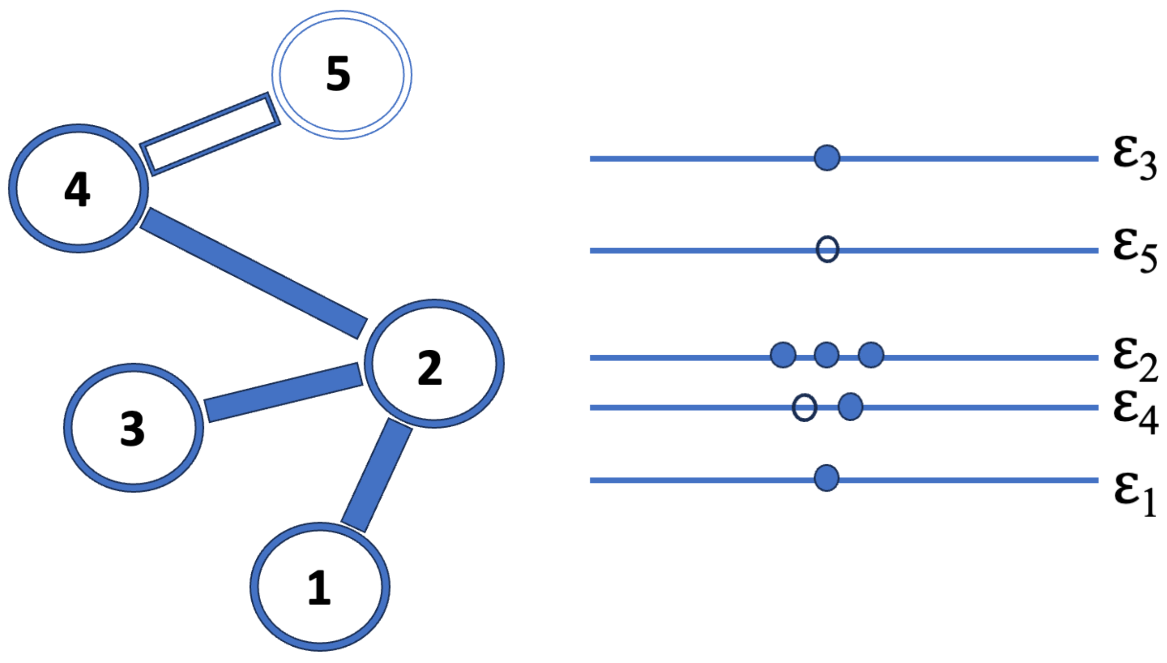
Figure 2.
A double-well potential to depict the system described by Eq. (3). Each individual particle in the double well follows a Langevin equation (cf. Eq. (13)). The energy levels of the left well, the barrier, and the right well are , , and , respectively. With Gaussian distributed thermal noise, Eq. (4) gives for classical particles and Eq. (6) gives this distribution for bosons. With Lévy noise, Eq. (16) gives for classical particles and Eq. (17) gives this distribution for bosons.
Disclaimer/Publisher’s Note: The statements, opinions and data contained in all publications are solely those of the individual author(s) and contributor(s) and not of MDPI and/or the editor(s). MDPI and/or the editor(s) disclaim responsibility for any injury to people or property resulting from any ideas, methods, instructions or products referred to in the content. |
© 2024 by the authors. Licensee MDPI, Basel, Switzerland. This article is an open access article distributed under the terms and conditions of the Creative Commons Attribution (CC BY) license (http://creativecommons.org/licenses/by/4.0/).
Copyright: This open access article is published under a Creative Commons CC BY 4.0 license, which permit the free download, distribution, and reuse, provided that the author and preprint are cited in any reuse.


