
Submitted:
28 December 2023
Posted:
29 December 2023
You are already at the latest version
Abstract
The new logic of partitions is dual to the usual Boolean logic of subsets (usually presented only in the special case to the logic of propositions) in the sense that partitions and subsets are category-theoretic duals. The new information measure of logical entropy is just the normalized quantitative version of partitions. The new approach to interpreting quantum mechanics (QM) is showing that the mathematics (not the physics) of QM is the Hilbert space version of the mathematics of partitions. Or putting it the other way around, the math of partitions is a skeletal version of the math of QM. The key concepts throughout this progression from logic to information theory to quantum theory are distinctions versus indistinctions, definiteness versus indefiniteness, or distinguishability versus indistinguishability. The distinctions of a partitions are the ordered pairs of elements from the underlying set that are in different blocks of the partition. Logical entropy is defined (initially) as the normalized number of distinctions. The cognate notions of definiteness and distinguishability run through the math of QM, e.g., in the key non-classical notion of superposition (= ontic indefiniteness) and in the Feynman rules for adding amplitudes (indistinguishable alternatives) versus adding probabilities (distinguishable alternatives).
Keywords:
logic of partitions
; logical entropy
; ontic indefiniteness
; indistinguishability
1. Introduction: Where Does QM Math Come from?
The mathematics of quantum mechanics (QM) is quite distinctive and different from the mathematics of classical physics. Where does that distinctive math of QM come from? The purpose of this paper is to expound a new way to interpret quantum mechanics (QM), or, to be more precise, to interpret the mathematics (not the physics) of QM.
One research program in the philosophy of quantum mechanics is “reconstruction” [30] which aims at new derivations of QM for both the new and distinctive math of QM and the physics usually obtained by quantization. The hope is that new and particularly perspicuous axioms may give hints about the ontology of QM. In our approach, only the math of QM is reconstructed as the Hilbert-space version of the math of partitions–and that alone is sufficient to see the type of objectively indefinite ontology described by that math. Quantization then shows the changes in classical physics to fit that new math frameworks, e.g., the De Broglie and Einstein relations.1 Our view is that thus treating the math and physics by those separate ways is “cutting at the joints” as opposed to the usual program of trying to reconstruct the math and physics of QM together.
In other approaches to the philosophy of QM, the modus operandi seems to be that the standard theory needs to be changed in order to be interpreted, e.g., Bohmian mechanics or spontaneous localization. The approach taken here is to provide a realistic interpretation of the standard non-relativistic finite-dimensional von Neumann/Dirac theory.
2. Materials and Methods
The key mathematical, indeed logical, concept is the notion of a partition on a set–or equivalently, the notion of an equivalence relation. The basic thesis is that the math of QM is the Hilbert space version of the math of partitions. Partitions are the basic logical concept to describe
- distinctions versus indistinctions,
- definiteness versus indefiniteness, and
- distinguishability versus indistinguishability.
The new logical information measure is just the quantitative version of partitions.
The key non-classical notion of state in QM is that of superposition–with entanglement being a particularly unintuitive special case.
Thus, superposition, with the attendant riddles of entanglement and reduction, remains the central and generic interpretative problem of quantum theory. [14], (27)
The result of the thesis is to give a partitional explication of superposition in terms of objective indefiniteness between definite alternatives–so that this approach to QM could be called the Objective Indefiniteness Interpretation of QM.2
From these two basic ideas alone – indefiniteness and the superposition principle – it should be clear already that quantum mechanics conflicts sharply with common sense. If the quantum state of a system is a complete description of the system, then a quantity that has an indefinite value in that quantum state is objectively indefinite; its value is not merely unknown by the scientist who seeks to describe the system. Furthermore, since the outcome of a measurement of an objectively indefinite quantity is not determined by the quantum state, and yet the quantum state is the complete bearer of information about the system, the outcome is strictly a matter of objective chance – not just a matter of chance in the sense of unpredictability by the scientist. Finally, the probability of each possible outcome of the measurement is an objective probability. Classical physics did not conflict with common sense in these fundamental ways. [55], (47)
Abner Shimony suggested calling this interpretation of the math or “formalism of quantum mechanics” as the Literal Interpretation.
These statements ... may collectively be called “the Literal Interpretation” of quantum mechanics. This is the interpretation resulting from taking the formalism of quantum mechanics literally, as giving a representation of physical properties themselves, rather than of human knowledge of them, and by taking this representation to be complete. [57], (6-7)
3. Results
3.1. The Lattice of Partitions
A partition on a set is a set of nonempty subsets or blocks that are mutually disjoint and jointly exhaustive (their union is U).3 An equivalent definition, that prefigures the Hilbert space notion of a “direct-sum decomposition” of the space in terms of the eigenspaces of a Hermitian operator, is a set of nonempty subsets such that every non-empty subset can be uniquely represented as the union of a set of nonempty subsets of the –in particular .
As the mathematical tool to describe distinctions versus indistinctions, a distinction or dit of is an ordered pair of elements of U in different blocks of the partition, and the ditset is the set of all the distinctions of (also called an “apartness relation”). An indistinction or indit of is an ordered pair of elements in the same block of the partition, and the indit set is the set of all indits of –which is the equivalence relation associated with whose equivalence classes are the blocks of .
The partial order on partition is usually defined as (where ) if for every , there is a such that , but it is easier to just define it by if . The join (least upper bound) and meet (greatest lower bound) operations on partitions on U form the partition lattice . The most important operation for our purposes is the join operation where the join is the partition on U whose blocks are the nonempty subsets for and . It could also be defined using ditsets since: .
The meet of and can be defined as the partition determined by the intersection of all the equivalence relations containing the equivalence relations corresponding to and .
The partition lattice also has a top and bottom. The top is the discrete partition with only singleton blocks which makes all possible distinctions, i.e., (where is the diagonal of self-pairs ). The bottom is the indiscrete partition (or “The Blob”4) with only one block U and it makes no distinctions so and .
In terms of the old notions of matter or substance and form, the bottom of the partition lattice has all the substance but no form (no dits). The quantum notion of distinction-making change is prefigured by moving up the partition lattice as the substance is increasingly in-formed by distinctions until finally reaching the classical state . As a metaphor for the Big Bang, in the beginning there was all the substance (energy) but with no distinctions, i.e., “perfect symmetry” [49], and then distinctions were introduced by symmetry-breaking to create (more definite) “its from dits.” That partition notion of becoming is particularly important for our purposes since it prefigures the notion of quantum (projective) measurement (von Neumann’s Type I processes) as well as quantum jumps.
The other logical notion of becoming or creating is illustrated by moving up the Boolean lattice of subsets. In the beginning, there was no substance (empty set) and then becoming takes place by the creation (ex nihilo) of “its” that are fully formed as illustrated in Figure 1.
Metaphors might help to conceptualize the difference between the classical notion of change and quantum notion of becoming. In a police book of mug shots, the faces are fully formed and a metaphor for classical change is flipping through the fully definite or determinate mug shots. The quantum notion of becoming is like the police artist’s sketch pad where the indefinite outline of a face becomes more and more definite. Or a white (superpositions of all colors) painter’s canvas becomes a painting as white superposition of colors “collapses” to take on definite colors. Since there are layers or levels of increasing definiteness as one moves up the lattice of partitions, another metaphor might be 3D printing where the printed object takes shape as the printer moves up to higher layers.
The mathematics for this transition from indefinite to more definite is the refining of partitions. The logical operation on partitions that results in a refinement is the join of partitions (i.e., the intersection of equivalence relations) which provides a skeletal model of quantum projective measurement. The mathematics of QM is the extension of that partition math to complex Hilbert space.
3.2. The Logic of Partitions
The partition join and meet operations were known in the nineteenth century (e.g., Dedekind and Schröder). Ordinary logic is based on the Boolean logic of subsets of a universe set U; propositional logic is the special case of a one element universe U. In subset logic, the formulas, in general, stand for subsets of some universe set U. And subsets (or generally subobjects or `parts’) are category-theoretically dual to partitions (or generally quotient objects). “The dual notion (obtained by reversing the arrows) of `part’ is the notion of partition.” [42], (85). Hence one would naturally expect there to be a dual logic of partitions, where the formulas stand for partitions on some universe set U. But that would require at least the operation of implication on partitions (corresponding to the Boolean conditional ), but no new operations on partitions were defined in the twentieth century. As acknowledged in a 2001 volume commemorating Gian-Carlo Rota: “the only operations on the family of equivalence relations fully studied, understood and deployed are the binary join ∨ and meet ∧ operations.” [10], (445) Only in the current century was the implication operation on partitions (which turns the partition lattice into an algebra) defined along with general algorithms to turn subset logical operations into partition logical operations. The resulting logic of partitions cemented the notion of a partition as not just a mathematical concept of combinatorics but a logical concept. ([18,23])
There is a parallel development of subset logic and partition logic based on the dual connection between the elements or “its” of a subset and the distinctions or “dits” of a partition–which is summarized in Table 1. At the mathematical level, the dual lattices or logics are equally fundamental.
In subset logic, a formula is valid if for any U ( ) and any subsets of U substituted for the atomic variables, the formula evaluates by the logical subset operations to the top U. Similarly in partition logic, a formula is valid if for any U () and any partitions on U substituted for the atomic variables, the formula evaluates by the logical partition operations to the top . The partition validities are a proper subset of the Boolean subset validities but are neither contained in nor contain the valid formulas of intuitionistic logic (Heyting algebras).
3.3. Logical Information Theory: Logical Entropy
In his writings (and MIT lectures), Gian-Carlo Rota further developed the parallelism between subsets and partitions by considering their quantitative versions: “The lattice of partitions plays for information the role that the Boolean algebra of subsets plays for size or probability.” [41], (30) Since the normalized size of a subset gives its Boole-Laplace finite probability, so the “size” of a partition would play a similar role for information:
.
Since “Probability is a measure on the Boolean algebra of events” that gives quantitatively the “intuitive idea of the size of a set”, we may ask by “analogy” for some measure “which will capture some property that will turn out to be for [partitions] what size is to a set.” [52], (67) The duality (represented in Table 1) tells us that it is the number of dits in a partition that gives its size (maximum at the top and minimum at the bottom of the partition lattice) that is parallel to the number of `its’ in a subset (maximum at the top and minimum at the bottom of the subset lattice).
That is the reasoning that motivates the definition of the logical entropy of a partition as the normalized size of its ditset (equiprobable points):
.
In general, if the points of have general positive probabilities , then , so that:
.
The parallelism carries through to the interpretation: is the one-draw probability of getting an `it’ of S and is the two-draw probability of getting a `dit’ of .
The logical entropy is a (probability) measure in the sense of measure theory, i.e., is the product measure on the ditset . As a measure, the compound notions of joint, conditional, and mutual logical entropy satisfy the usual Venn diagram relationships.
The well-known Shannon entropy can also be interpreted in terms of partitions; it is the minimum average number of binary partitions (bits) it takes to distinguish the blocks of . The Shannon entropy is not a measure in the sense of measure theory but the compound notions of joint, conditional, and mutual Shannon entropy were defined so that they satisfy similar Venn-like pictures (but with no underlying set). That is possible because there is a non-linear but monotonic dit-to-bit transform, i.e., , that takes to and which preserves Venn diagrams [22].
If a partition is the inverse-image partition of a numerical attribute , then is the two-draw probability of getting different f-values. The notion of logical entropy generalizes naturally to the notion of quantum logical entropy ([22]; [60]) where it gives the probability in two independent measurements of the same state by the same observable that the result gives different eigenvalues.
3.4. Partitions as Skeletonized Quantum States
There is a very simple way to skeletonize a quantum state to arrive at the corresponding set notion. Consider as both a set of distinct points and also as a orthonormal basis for a 4-dimensional Hilbert space. Then a superposition state vector of the form (say) is skeletonized by deleting the complex scalars and , the Dirac kets, and the addition operation to yield just the support, the set as a block in a partition, i.e., vector in QM math ⇝ support in partition math. A superposition of states skeletonizes to elements in the same block of a partition, i.e., superposition = indistinction (which is non-trivial in the sense of not being a diagonal pair like ). Figure 2 is the lattice of partitions starting with a pure state (indiscrete partition), non-classical mixed states (i.e., mixed states containing at least one superposition), and the classical mixed state (where we have used the partition shorthand of representing the partition as i.e., the inner-most curly brackets are eliminated in favor of juxtaposition). The interpretation is that are distinct definite- or eigen-states of a particle according to some observable, where “particle” does not mean a classical (or Bohmian) particle but an entity that can have different levels of objective indefiniteness (superpositions of the eigenstates such as or d) or the definiteness of an eigenstate.5
Figure 2 is the Hasse diagram of the partition lattice on a four element set which means that each line between two partitions represents the partial order of refinement with no intermediate partitions. Then the change from a partition to a more refined one is a “jump.” The skeletonized mixed states in the lattice of partitions of Figure 2 are all those that might be obtained by a “projective measurement” of the pure state , i.e., by the partition join version of the Lüders mixture operation. All the lines or links in Figure 2 go from an indefinite state upward to a more definite state that is part of a join operation. A projective measurement turns a pure state into a mixed state one part of which, e.g., an eigenstate in a maximal measurement, is realized according to its probability.
The set level precursor of such a quantum jump from a superposition to an eigenstate is the “choice function” [31], (60) which assigns to each nonempty subset (like a block in a partition) an element of the subset. That determination of an element is non-deterministic except in the special case of a singleton set which is the precursor of the quantum measurement when the outcome has probability one, namely when the state being measured is a single eigenstate of the observable being measured as indicated in Table 2.
The indeterminism of the jump in the set level choice function shows that those indeterminate aspects of QM math are even prior to the introduction of probabilities.
The top discrete partition is the skeletal version of a classical mixed state like randomly choosing a leaf in a four-leaf clover or randomly choosing a `letter’ in the four-letter genetic code . One criterion of classical reality was the idea that it was fully definite or definite all-the-way-down as in Leibniz’s Principle of Identity of Indistinguishables (PII) [5], (Fourth letter, 22) or Kant’s Principle of Complete Determination (omnimoda determinatio).
Every thing, however, as to its possibility, further stands under the principle of thoroughgoing determination; according to which, among all possible predicates of things, insofar as they are compared with their opposites, one must apply to it. [37], (B600)
Thus two distinct things must have some predicate to distinguish them or if there is no way to distinguish them, then they are the same thing. This principle of classicality characterizes the `classical’ state :
For any , if , then
Partition logical version of Principle of Identity of Indistinguishables.
Any non-classical state in the skeletal representation is a partition with a non-singleton `superposition’ block, e.g., so but .
In contrast, quantum reality is not definite all-the-way-down. A state could even be maximally specified and still leave room for many particles (bosons) to be in that state.
In quantum mechanics, however, identical particles are truly indistinguishable. This is because we cannot specify more than a complete set of commuting ob servables for each of the particles; in particular, we cannot label the particle by coloring it blue. [53], (446)
In addition to PII, Leibniz had other metaphysical principles characteristic of the classical notion of reality. His Principle of Continuity was expressed by “Natura non facit saltus” (Nature does not make jumps) [43], (Bk. IV, chap. xvi) and his Principle of Sufficient Reason was expressed as the statement “that nothing happens without a reason why it should be so rather than otherwise” [5], (Second letter, 7). All these classical principles are violated in the quantum world; PII is violated by superpositions of bosons, Continuity is violated by the quantum jumps, and Sufficient Reason is violated by the objective probabilities of QM.
This skeletal representation of quantum states is summarized in Table 3.
4. Superposition as Indefiniteness in the Quantum `Underworld’
The biggest `enemy’ to understanding QM is the wave imagery, not to mention the name “wave mechanics.” That imagery interprets superposition ontologically as the sum of two waves to give another wave as in Figure 3.
The mathematics of waves is always present since any vector in a space over the complex numbers automatically has wave imagery in the polar representation as having an amplitude and phase. But the physical interpretation of waves is a misleading artefact or by-product of the use of complex numbers in the math of QM. The complex numbers are used because (among other reasons) they are algebraically complete so that the observable operators will have a complete set of eigenvectors [64], (67, fn. 7),6 It is a fact of the mathematics that the addition of vectors in a vector space over can always be represented as the superposition of waves with interference effects.
The wave formalism offers a convenient mathematical representation of this latency, for not only can the mathematics of wave effects, like interference and diffraction, be expressed in terms of the addition of vectors (that is, their linear superposition; see [26], (Chap. 29.5)), but the converse, also holds. [36], (303)
On the partitional approach, a superposition of two definite- or eigen-states states and is a state that is ontically indefinite or “blurred” between the two definite states. The partition approach requires the mental change-over from superposition-as-wave-addition to superposition-as-indefiniteness (since partitions are the math tool to describe indefiniteness and definiteness). Quantum reality is Indefinite World.
For a pictorial image, the left side of Figure 4 gives the superposition of two isosceles triangles with labelled edges and vertices as the triangle that is indefinite on the edges and vertices where they differ and only definite where the two triangles are the same–and certainly not the triangle that is doubly definite (like a double-exposure photograph). Forget waves an ontological entities; instead think of objective indefiniteness.
The fact that where superposed states have the same property is still definite (like vertex label a, the side label A) in the superposition is a little noticed fact about quantum superpositions.
It follows from the linearity of the operators which represent observables of quantum mechanical systems that any measurable physical property which happens to be shared by all of the individual mathematical terms of some particular superposition (written down in any particular basis) will necessarily also be shared by the full superposition, considered as a single quantum-mechanical state, as well. [4], (234)
This means that the notion of superposition in QM is the flip-side of the notion of abstraction (e.g., in mathematics) [21].7 In a superposition, the emphasis is on the indefiniteness resulting from where the elements of a set (i.e., a non-singleton equivalence class in an equivalence relation) differ like the vertex labels b and c, and the side labels B and C in Figure 4, while in abstraction, the emphasis is on the properties that are the same for the elements in the set (or equivalence class) like the vertex label a and side label A. It is like the flip-side different viewpoints of seeing the same glass as half-empty or as half-full.
In the older homotopy theory, the abstraction of a “homotopy type” was represented by a block in a partition, i.e., by an equivalence class. “Homotopy types are equivalence classes of spaces” under the equivalence relation “of deformation or homotopy.” [7], (4). In the modern treatment [61], the equivalence class of, say, unit-interval-coordinatized paths going once around the ring clockwise (right side of Figure 4) is abstracted to an object having those common characteristics but is not itself one of the differing paths in the equivalence class.
This insight that superposition as indefiniteness-on-differences is the flip-side of abstraction as definiteness-on-commonalities is, of course, unavailable when superposition is thought of as wave-addition.
Any quantum theorist who realizes that a superposition in the measurement basis does not have a definite value prior to the measurement–already has a strong hint as to the nature of quantum reality. Some quantum theorists have taken the hint and envisioned a quantum world characterized by that indefiniteness where that “blurriness is an ontic feature” [50], (p. 163). Thus it is not a new idea that there is a quantum `underworld’ of indefinite superposition states `beneath’ the classical space-time world of definite states. That view was often expressed in the language of the quantum world of potentialities (or latencies) versus the classical world of definite actualities ([34]; [47]; [36], (Sec. 10.2); [57]; [29]; [35], (Quantum Reality #8); [38,40]; [15]).
Heisenberg [34], (53)... used the term “potentiality” to characterize a property which is objectively indefinite, whose value when actualized is a matter of objective chance, and which is assigned a definite probability by an algorithm presupposing a definite mathematical structure of states and properties. Potentiality is a modality that is somehow intermediate between actuality and mere logical possibility. That properties can have this modality, and that states of physical systems are characterized partially by the potentialities they determine and not just by the catalogue of properties to which they assign definite values, are profound discoveries about the world, rather than about human knowledge. [57], (6)
Ruth Kastner uses the imagery of an iceberg [38], (3) with the classical world above water and the quantum world beneath the water—an imagery that is filled out by the Figure 2 imagery of the partition lattice as the skeletonized classical and quantum states. The language of “potentialities” or the Aristotelian notion of “potentia” is not very felicitous since they are taken to be realities, not mere possibilities. Hence some prefer the language of “latencies” (e.g., Henry Margenau and R. I. G. Hughes), but in both the cases of “potentialities” and “latencies,” the key idea is objective indefiniteness.
The historical reference should perhaps be dismissed, since quantum mechanical potentiality is completely devoid of teleological significance, which is central to Aristotle’s conception. What it has in common with Aristotle’s conception is the indefinite character of certain properties of the system. [56], (313-4)
And Margenau notes that the measurement of observables “forces them out of indiscriminacy or latency” [47], (10)–which indicates that Margenau also interprets “latency” in terms of indeterminacy or indefiniteness. Kastner also considers the indeterminacy of values as a key characteristic of the real potentia [38], (3). “Although the quantum possibilities represent properties that might be observed, they are not determinate (that is, they are not well defined).” [39], (27) In short, it is not real potentialities versus real actualities, but real (objective) indefiniteness versus real definiteness. There is only one type of reality and it occurs in varying degrees of indefiniteness as represented in skeletal form by the partition lattice (Figure 2).
The main brain-twisting reconceptualization required to understand quantum reality is:
- to replace the classical notion of fully definite reality by the idea of indefiniteness at the quantum level (not definite all-the-way-down),
- where the state-reduction jump from an indefinite state to a more definite state is due to making distinctions (“more-definite its from dits”), and
- where change with no distinctions stays at the same level of indefiniteness (unitary evolution)
. Classical mechanics has only one type of change, definite to definite at the level of fully definite classical reality.
After a century of the philosophically fruitless conceptualization of QM states in terms of wave functions, is there another equivalent mathematical tool to represent a quantum state that makes the indefiniteness obvious? Yes, it is the density matrix.
4.1. Quantum States
To demonstrate our thesis that the math of QM is the Hilbert space version of the math of partitions, we need to first focus on the three main concepts in the math of QM: 1) the quantum state, 2) the quantum observable, and 3) the quantum ( always projective) measurement.
A quantum state can be presented either as a state vector or as a density matrix [63]. The density matrix approach best displays the relevant information for the partitional interpretation in terms of indefiniteness. Hence we start by transferring the structure of a partition into its density matrix form . The initial data is a partition on U with (positive) point probabilities . For each , define as the column vector with the entry being if , else 0 so that . We form the projection density matrix with the -entry being if , else 0. It should be noted how the indefiniteness interpretation of superposition comes out in the mathematics. The set-level superposition of and in implies the non-zero off-diagonal element in indicating indefiniteness.
These density matrices of pure superposition states also show the origin of the Born rule in the outer product construction of a pure state density matrix. Taking , an arbitrary non-empty subset of U, the entry of is . Then the probability of conditioned on S is given by the Born rule: .8
Returning to the partition , the density matrix is the probability sum of these projectors:
.
Then it is easily checked that if , else 0. Thus the non-zero entries in represent the indits of and the zero entries represent the distinctions of . A density matrix is not only Hermitian but positive so its eigenvalues are non-negative real numbers which sum to 1, i.e., . In the case of , these are m non-zero eigenvalues with the remaining eigenvalues of 0.
For the classical state , its density matrix is a diagonal matrix with the point probabilities along the diagonal, e.g. “the statistical mixture describing the state of a classical dice before the outcome of the throw” [6], (176). Thus the non-classical states in the skeletal representation are the ones where has non-zero off-diagonal elements indicating the `amplitudes’ of the corresponding diagonal states ( and ) blobbing or cohering together in a superposition. Since superposition states are the key non-classical states, it is these non-zero off-diagonal “coherences” [13], (303) that account for the non-classical interference effects in the Hilbert space version.
[T]he off-diagonal terms of a density matrix ... are often called quantum coherences because they are responsible for the interference effects typical of quantum mechanics that are absent in classical dynamics. [6], (177).
In the full non-skeletal Hilbert space case of a density matrix , it has a spectral decomposition with an orthonormal basis so and where the non-negative eigenvalues sum to 1. Thus for the concept of a quantum state, we have the skeletal set level presentation of a partition and the corresponding Hilbert space version of that partition math as summarized in Table 4.
4.2. Quantum Observables
We have seen how the notion of a quantum state was prefigured at the set level by (i.e., has the set level precursor of) a partition on a set with point probabilities. In a similar manner, the notion of a quantum observable is prefigured at the set level by the inverse-image partition of a real-value numerical attribute .
In the folklore of mathematics, there is a semi-algorithmic procedure to connect set concepts with the corresponding vector (Hilbert) space concepts. We will call it a “yoga” [51], (251), the Yoga of Linearization:
For any given set-concept, apply it to a basis set of a vector space
and whatever is linearly generated is the corresponding vector space concept.
The Yoga of Linearization.
To apply the Yoga, we first take U as just a universal set and consider some set-based concept, and then we consider U as a basis set (e.g., ON basis of a Hilbert space) of a vector space V and see what is linearly generated. Starting with U, it is just the free vector space functor that takes a set to the free vector space over a given field which we take to be . A subset S of a basis set U generates a subspace of the space V. The cardinality of the subset gives the dimension of the subspace. A real-valued numerical attribute defines a Hermitian operator (where ) by defining F on the basis set U as or, using the fancier notation, .
To better analyze the numerical attribute, let stand for “the value of f on the subset S is r”. That is the set level version of the eigenvalue/eigenvector equation . Hence we see that the set version of an eigenvector is a constant set S of f and the set version of an eigenvalue of an eigenvector is the constant value r on a constant set S. A characteristic function has only two constant sets and . The Yoga yields the corresponding vector space notion which is a projection operator which is defined by if , else (zero vector) which has the eigenvalues of 0 and 1.
A Hermitian (or self-adjoint) operator F in QM has spectral decomposition where the sum is over the real eigenvalues and the projections to their eigenspaces. Bearing in mind the correlation given by the Yoga, we can define the `spectral decomposition’ of the numerical attribute as . Starting at the quantum level with a Hermitian operator and a basis set U of eigenvectors of F, then going backwards to the set level, f is obtained as the eigenvalue function .
An important application of the Yoga is to the notion of a set partition as the inverse-image of a numerical attribute. Applied to the basis set used to define F by , each block of generates the eigenspace of eigenvectors for the eigenvalue r. These eigenspaces form a direct-sum decomposition (DSD) of V, i.e., , where a DSD is defined as a set of non-zero subspaces such that every non-zero vector has a unique representation as a sum of vectors .9
It was noted previously that a set partition has a similar definition since every non-empty subset S has a unique representation as the union of subsets of the . If the union of the ’s was not all of U, then would have no representation, and if , then S has two representations as subsets of the ’s. Moreover, is a projection operator that takes any subset to . Thus we have whose quantum version is resolution of unity . And lastly, we might apply the Yoga to the Cartesian product where U and are basis sets for V and . Then the ordered pairs (bi)linearly generate the tensor product where the ordered pair is customarily written as or .
These results of the Yoga of Linearization are summarized in Table 5 further showing how the math of QM is the Hilbert space version of partition math at the skeletal level of sets.
4.3. Quantum Measurement
The third basic concept to be analyzed is quantum measurement (always projective)–the quantum notion of becoming, i.e., change going from a level of indefiniteness to a level of more definiteness. The connection between the set level notion of measurement and the quantum level is the Lüders mixture operation ([45]; [6], (p. 279)) that can be applied at both levels. At the set level, we have the skeletal state represented by a density matrix and we have an `observable’ or real-value numerical attribute, say, whose inverse-image is the partition . The Lüders mixture operation applies the `observable’ to the density matrix to arrive at the post-measurement density matrix . The operation uses the projection matrices for the blocks of which are diagonal matrices whose diagonal elements are the values of the characteristic function . Then the post-measurement density matrix is:
Partition version of Lüders mixture operation.
Then it is an easy result:
Theorem: .
Thus the set version of quantum level projective measurement in the math of QM is the partition join operation where and, by DeMorgan’s Law, so the join of partitions operation can also be viewed as the intersection of equivalence relations. The non-classical quantum notion of becoming is the jump from to the mixed state and then to one of the states in the mixture according to its probability.
Example: Let with probabilities , , and in and so for any that assigns the same g-value to a and b with a different value for c. Then the density matrix for and the projections matrices for the blocks of are:
, , and .
The Lüders mixture operation is:
.
Since , we see that the post-measurement density matrix is . Thus the superposition of and in got distinguished since b and c had different g-values. The new distinctions in are (along with ) and those were the non-zero off-diagonal elements (coherences) of that got zeroed (distinguished or decohered) in . Figure 5 shows the join of and is their least upper bound .
In the math of the partition join, the partitions are symmetrical. But the Lüders mixture operation is not symmetric even through the result is the join. One partition () represents the state being measured and the other partition () represents the observable. Since the join in Figure 5 is the discrete partition, the measurement represented by the join is maximal. The arrow in Figure 5 represents the jump from a less refined mixed state to the maximal state .
The Lüders mixture is not the end of the measurement process. The measurement returns one of the g-values, say the (degenerate) one for . Then the Lüders Rule [36], (Appendix B) gives the final density matrix which is the corresponding term in the Lüders mixture sum, e.g., , normalized so the final density matrix is the (in this case, classical) mixed state:
.
In the general Hilbert space case, the Hermitian operator G is given by its DSD of eigenspaces (where is the eigenvalue function assigning the appropriate real eigenvalue to each vector in an ON basis U of eigenvectors of G). The state being measured is given by density matrix expressed in the ON basis U, and the Lüders mixture operation uses the projection matrices to the eigenspaces of G to determine the post-measurement density matrix . The Hilbert space version of the set operation is:
Hilbert space version of Lüders mixture operation.
We saw previously how the notion of logical entropy (and its quantum counterpart) was based on the notion of a quantitative measure of distinctions of a partition. Hence logical entropy is the natural notion to measure the changes in a density matrix under a measurement. For instance, in the above example where , the block probabilities are and , and the logical entropy is: . When the partition is represented as a density matrix , then the logical entropy could also be computed as:
The logical entropy is the two-draw probability of drawing a distinction of so it could also be computed as the sum of all the distinction probabilities (remembering that a distinction is an ordered pair of elements in different blocks so the probability of an unordered pair is doubled). Hence in general we have: , or in the case at hand:
.
There is then a general theorem [22] showing how logical entropy measures measurement.
Theorem (set case of measuring measurement): The increase in logical entropy from to in the Lüders mixture operation , is the sum of the squares of the off-diagonal non-zero entries in that were zeroed in the measurement operation .
In the example, the logical entropy of the post-measurement state is:
.
The sum of the squares of the non-zero off-diagonal terms (representing the coherences) of that were zeroed (decohered) in is:
and the increase in logical entropy due to the making of distinctions is:
.
And the quantum case follows mutatis mutandis.
Theorem (quantum case of measuring measurement): In the Lüders mixture operation , the increase in quantum logical entropy from to is the sum of the absolute squares of the off-diagonal entries in that were zeroed in the measurement operation .
The dictionary relating the three basic concepts in the math of QM to their set partitional precursors is given in Table 6.
4.4. Other Aspects of QM Mathematics
4.4.1. Commuting, Non-Commuting, and Conjugate Operators
We have seen that a Hermitian operator is the QM math version of a real-valued numerical attribute and that the direct-sum decomposition of the operator’s eigenspaces is the QM math version of the inverse-image partition of the numerical attribute. Let be two Hermitian operators with the corresponding DSDs of and . Since the two DSDs are the vector space version of partitions, consider the join-like operation giving the set of non-zero subspaces formed by the intersections . The additional generality gained over the join of set partitions is that these subspaces may not span the whole space V. Since the vectors in those intersections are simultaneous eigenvectors of F and G, let be the subspace spanned by the simultaneous eigenvectors of F and G. The commutator is a linear operator on V so it has a kernel consisting of the vectors v such that . Then there is a:
Theorem: . [24]
Since commutativity is defined as , we have the following definitions in terms of the vector space partitions or DSDs:
- F and G are commuting if ;
- F and G are incompatible if ;
- F and G are conjugate if (zero space).
Since the join-like operation on DSDs yields a set of subspaces that do not necessarily span the whole space, that operation is only the join of DSDs in the commuting case–or as Hermann Weyl put it: “Thus combination [join] of two gratings [DSDs] presupposes commutability...” [65], (257).
The set version of compatible partitions for the join operation is simply being defined on the same set. Hence our thesis gives a complete parallelism between compatible partitions and commuting operators.
Partition math: A set of compatible partitions defined by is said to be complete, i.e., a Complete Set of Compatible Attributes or CSCA, if their join is the partition whose blocks are of cardinality one (i.e., ). Then the elements are uniquely characterized by the ordered set of values .
QM math: A set of commuting observables is said to be complete, i.e., a Complete Set of Commuting Observables or CSCO [16], (57), if the join of their eigenspace DSDs is the DSD whose subspaces are of dimension one. Then the simultaneous eigenvectors of the operators are unique characterized by the ordered set of their eigenvalues.
This is a particularly clear case of showing that the QM math is a word-for-word translation (using the Yoga dictionary) of partition math.
4.4.2. Feynman’s Treatment of Measurement
The partitional approach to understanding the math of QM shows that the key organizing concepts are indistinction versus distinction, indefiniteness versus definiteness, or indistinguishability versus distinguishability. Those concepts define the notion of logical entropy in the new partition-logical theory of information-as-distinctions ([22]; [46]). When a particle in a superposition state undergoes an interaction, what characterizes whether it is a measurement or not? As early as 1951 [25], Richard Feynman gave the analysis of “measurement or not” in terms of distinguishability.
If you could, in principle, distinguish the alternative final states (even though you do not bother to do so), the total, final probability is obtained by calculating the probability for each state (not the amplitude) and then adding them together. If you cannot distinguish the final states even in principle, then the probability amplitudes must be summed before taking the absolute square to find the actual probability.[27], (3-9)
This analysis has been further explained by John Stachel.
Feynman’s approach is based on the contrast between processes that are distinguishable within a given physical context and those that are indistinguishable within that context. A process is distinguishable if some record of whether or not it has been realized results from the process in question; if no record results, the process is indistinguishable from alternative processes leading to the same end result. [58], (314)
The same points are restated by Anton Zeilinger using, in effect, the notion of information-as-distinctions.10
In other words, the superposition of amplitudes ... is only valid if there is no way to know, even in principle, which path the particle took. It is important to realize that this does not imply that an observer actually takes note of what happens. It is sufficient to destroy the interference pattern, if the path information is accessible in principle from the experiment or even if it is dispersed in the environment and beyond any technical possibility to be recovered, but in principle still “out there.” The absence of any such information is the essential criterion for quantum interference to appear. [68], (484)
What Feynman calls “distinguishability,” Zeilinger calls “information” since as one of the founders of quantum information theory, Charles Bennett, put it, information “is the notion of distinguishability abstracted away from what we are distinguishing, or from the carrier of information.... [8], (p. 155)
Feynman gives a number of examples ([27], (§ 3-3); [28], (17-8)) such as a particle scattering off the atoms in a crystal. If there is no physical record of which atom the particle scattered off of (i.e., the indistinguishable case), then no measurement took place so the amplitudes for the superposition state of scattering off the different atoms are added to compute the amplitude of the particle reaching a certain final state. But if all the atoms had, say spin up, and scattering off an atom flipped the spin, then a physical record exists (i.e., the distinguishable case) so a measurement took place11 and the probabilities of scattering off the different atoms are added to compute the probability of reaching a certain final state.
The same analysis applies to the well-known double-slit experiment where the distinguishable case is where there are detectors at the slits and the indistinguishable case is having no detectors at the slits. But the important thing to notice about Feynman’s example is that the measurement is entirely at the quantum level; it involves no macroscopic apparatus. Hence the Feynman analysis bypasses the whole tortured literature trying to analyze measurement in term of the “decoherence” induced by a macroscopic measuring devices (e.g., [69]). Of course, the quantum level physical record in the distinguishable case has to be amplified for humans to record the result but such macroscopic considerations have no role in quantum theory.
The implicit principle in Feynman’s analysis of measurement is:
If the interaction distinguishes between superposed eigenstates,
then a distinction (state reduction) is made.
The State Reduction Principle
The mathematics of the State Reduction Principle can be stated in both the set case and the QM case.
Theorem(State Reduction Principle–set case). Measurement is described in the set case by the Lüders mixture operation . The State Reduction Principle then states: if an off-diagonal entry (i.e., and are in a same-block superposition), then: if (i.e., the interaction distinguishes and ), then (i.e., the `coherence’ between and is decohered and a distinction is made).
Theorem(State Reduction Principle–QM case). Measurement is described in QM by the Lüders mixture operation (measuring by G). The State Reduction Principle then states: if an off-diagonal entry (i.e., the G-eigenvectors and are in a superposition in ), then: if and have different G-eigenvalues (i.e., the vectors are distinguished by G), then (i.e., the vectors are decohered12 and a distinction is made).
If no distinctions were made by the interaction, then no measurement took place.
4.4.3. Von Neumann’s Type I and Type II Processes
John von Neumann (vN) [62] made his famous distinction between the processes:
- (1)
- Type I process of measurement and state reduction, and
- (2)
- Type II process obeying the Schrödinger equation.
We have seen that the Type I processes of measurement involves distinguishability, i.e., the making of distinctions (like which atom the particle scattered off of), so a natural way to designate the Type II processes would be ones that do not make distinctions by preserving distinguishability or indistinguishability. The measure of indistinctness of two quantum states is their overlap or inner product. For instance, two states have zero indistinctness (zero inner product) then they are fully distinct (orthogonal). Hence the natural characterization of a Type II process is one that preserves inner products, i.e., a unitary transformation.13
The partitional approach highlights the key analytical concepts of indistinctions versus distinctions and the cognate notions of indefiniteness versus definiteness or indistinguishability versus distinguishability. Many people working on quantum foundations seem to ignore those key concepts, and then the division between the measurement and unitary evolution seems unfounded, if not “unbelievable.”
[I]t seems unbelievable that there is a fundamental distinction between “measurement” and “non-measurement” processes. Somehow, the true fundamental theory should treat all processes in a consistent, uniform fashion. [48], (245)
4.4.4. Hermann Weyl’s Imagery for Measurement
An industrial sieve is used to distinguish particles of matter of different sizes so it might serve as a helpful metaphor for the quantum process of making distinctions, namely measurement.
In Einstein’s theory of relativity the observer is a man who sets out in quest of truth armed with a measuring-rod. In quantum theory he sets out armed with a sieve. [17], (267)
Hermann Weyl quotes Eddington’s passage [65], (255) but uses his own expository notion of a “grating.” Weyl in effect uses the Yoga from the mathematical folklore to develop both the set notion of a grating as an “aggregate [which] is used in the sense of `set of elements with equivalence relation.”’ [65], (239) and the vector space notion of a direct-sum decomposition. In the set to vector space move of the Yoga, the “aggregate of n states has to be replaced by an n-dimensional Euclidean vector space” [65], (256). The notion of a vector space partition or “grating” in QM is a “splitting of the total vector space into mutually orthogonal subspaces” so that “each vector splits into r component vectors lying in the several subspaces” [65], (256), i.e., a DSD. After thus referring to a partition and a DSD as a “grating” or “sieve,” Weyl notes that “Measurement means application of a sieve or grating” [65], (259), i.e., the making of distinctions by the join-like process described by the Lüders mixture operation.
This imagery of measurement (or non-measurement) as passing through a sieve or grating is illustrated in Figure 6.
One should imagine the roundish blob of dough as the superposition of the definite shapes in the grating or sieve. The interaction between the superposed blob and the sieve/grating forces a distinction in the state reduction case, so a distinction is made as the blob must pass through one of the definite-shaped holes. In general, a state reduction (`measurement’) from an indefinite superposition to a more definite state takes place when the particle in the superposition state undergoes an interaction that distinguishes the superposed states. If the grating did not distinguish between the alternatives, than no state reduction takes place in the transition from position A to B (unitary evolution) as in the Feynman rule for the indistinguishable alternatives case.
4.5. A Skeletal Analysis of the Double-Slit Experiment
Consider the skeletal case of a particle have three possible states which are interpreted as vertical positions in the setup for the double-slit experiment in Figure 7.
In the set level skeletal analysis, we have discarded the scalars from but we are nevertheless left with the scalars 0 and 1 which are the elements of the field . There is the natural correspondence between the zero-one vectors in the three-dimensional vector space (i.e., the column vectors is associated with , and so forth) which establishes an isomorphism: , where the set addition is the symmetric difference, i.e., for , [19]. That mimics the addition mod 2 in since, for instance, . For our dynamics, we assume a non-singular linear transformation , , and which is non-singular since , , and also form a basis set for –so we also have a partition lattice on the basis set .
We are interested in the analysis when the particle arrives at the screen in the superposition , or in skeletal terms .
Case 1: There are detectors at the slits to distinguish between the two superposed states so the state reduces to the half-half mixture of and . Then evolves by the non-singular dynamics to which hits the wall and reduces to or with half-half probability. Similar evolves to which hits the wall and reduces to or with half-half probability. Since this is the case of distinctions between the alternative paths to , , or we add the probabilities to obtain:
.
.
.
Hence the probability distribution in the Case 1 of measurement at the screen is given in Figure 8.
Case 2: There are no detectors to distinguish between the slits in the superposition so it linearly evolves by the dynamics: . Hence the probabilities at the wall are:
.
.
.
Hence the probability distribution in the Case 2 of no distinctions at the screen is given in Figure 9.
The Case 2 distribution shows the usual probability stripes due to the interference in the linear evolution of the superposition state , i.e., the destructive interference in the evolved superposition .
Our classical intuitions insist on asking: “Which slit did the particle go through in Case 2?”. That question assumes that the evolution of the state was at the classical level where the slits were distinguished. But in Case 2, the slits were not distinguished so the evolution took place at the lower level in the skeletal lattice of partitions. In Figure 10, the Case 2 (and vN Type II) evolution (solid arrow) is illustrated as going from the superposition state in the partition lattice of states on to the superposition state lattice of states on . The Case 1 (and vN Type I) becoming (dashed arrows) does not take place with no detection at the slits.
The important `take-away’ is that there are different levels of indefiniteness (as illustrated in the partition lattice) and evolution can take place at a non-classical level of indefiniteness so, in that case, there is no matter of fact of the particle going through one slit or the other at the classical level.
Sometimes metaphors can serve as an aid or crutch to our biologically evolved intuitions. Suppose we have a fence across a field with two gates (like in the double slit experiment). When the sun is shines, that is a metaphor for detecting which gate a creature may walk through to get from A to B. Our creature is Hegel’s Owl of Minerva who only flies at night [33], (p. 13). Hence when the sun shines, the owl is limited to “flatland” [1] so it has to go through one gate of another to get from A to B as in Figure 11.
But when the sun sets, the Owl of Minerva’s “flights and perches” [32], (198) can go from ground perch A to ground perch B without going through one gate or the other as in Figure 12.
Our classical (“flatlander”) intuitions see only the definite ground-level paths or trajectories and, in the absence of the projecting light source (or sun) as in Case 2 above, will insist on asking: “Which gate did the owl go through?”. Our intuitions insist: “Why can’t I always imagine what happened at the classical level of fully distinguished states?”. But with no detections at the slits in the double-slit experiment, there is no matter of fact of the particle going through a slit at the classical level since the evolution is at the non-classical quantum level as in Figure 10 (illustrated by the third dimension in our flatlander metaphor of Figure 12).
Quantum states are built from below, as it were, through being in-formed by information-as-distinctions. Von Neumann’s two processes separate the Type I becoming from below between levels of indefiniteness and the Type II unitary evolution at the same level of indefiniteness. Figure 10 shows how quantum evolution transforms one superposition into another at the same level of indefiniteness (which allows interference) without any becoming or rising to the level of classical fully distinguished states. That is hard to understand for those who insist on “interpreting” QM with only our evolved intuitions based on the macroscopic (superposition-less) world.
5. Discussion
Our thesis is that the math of QM is the Hilbert space version of the math of partitions, or, put the other way around, the math of partitions is the skeletonized version of QM math. There are many other aspects of QM math that could be investigated such as group representations on sets or on vector spaces over since a group is essentially a `dynamic’ algebraic way to define an equivalence relation or DSD ([65], (73); [12]) (e.g., the orbit partition in a set representation or the DSD of irreducible subspaces in the vector space over representation). But in this introductory treatment, we have hopefully analyzed enough aspects of QM math to illustrate our thesis.
The main mystery in QM is superposition (entanglement being a particularly mysterious special case) and the quantum state of becoming wherein a superposition state jumps to a more definite state by being in-formed by distinctions. The rules governing when an interaction involving a superposition constitutes a state reduction or not, are given by the Feynman rules based on the notion of distinguishability or indistinguishability. At the logical level, the mathematics of distinguishability versus indistinguishability (or distinctions versus indistinctions) is the math of partitions. The quantitative version of partitions gives the notion of logical entropy that is the measure of information-as-distinctions so that in the Type I measurement process, distinctions in-form an indefinite state to jump to a more definite state.14 In contrast to the usual imagery of superposition as the addition of waves, the notion of ontological indefiniteness provides the alternative characteristic feature of non-classical superposition states.15
But, it will be said, “from the logical viewpoint, a property or the complementary property has to definitely apply to a particle.” That is the viewpoint of the classical logic of subsets; an element has to be in a subset or in its complement; there is no indefiniteness. There is, however, an equally fundamental logic at the mathematical level, the dual logic of partitions.16 In a (non-discrete) partition on the definite- or eigen-states of an observable, each non-singleton block represents the (skeletonized version) of objective indefiniteness of those eigenstates in the block. In a state reduction, distinctions are made to create more definiteness–with the classical mixed state of fully distinguished states being the maximal result. That is the notion of becoming described in partition logic, not the sort of transformations considered in classical physics, not to mention the classical logic of subsets.
Subsets and partitions are equally fundamental (indeed, dual) logical concepts. The notion of partitions (or equivalence relations) is the logical concept to describe indistinctions versus distinctions, indistinguishability versus distinguishability, or indefiniteness versus definiteness. Thus the partitional approach to QM does not use some jury-rigged concepts (e.g., Bohmian mechanics or spontaneous localization theory) to have yet another “interpretation” of QM. It should not be surprising that fundamental logical concepts can explicate the fundamental physical theory. [67]
This approach to better understanding or interpreting QM works with the standard von Neumann/Dirac quantum theory. It does not involve any new physics, unlike the pilot-wave or spontaneous localization theories. In that sense, the partitional approach shows how to develop Shimony’s idea of the Literal Interpretation of the math or “formalism of quantum mechanics” [57], (6-7). Furthermore, the partitional analysis substantiates the analysis of Heisenberg, Shimony, and others which describes the quantum world in terms of potentialities or latencies, where, in both cases, the key attribute was the reality of objective indefiniteness.17
- Superposition is the key non-classical notion of state in QM math;
- objective indefiniteness is its ontological counterpart;
- the quantum notion of becoming (vN Type I) is the jump from an indefinite state to a more definite state; and
- the quantum notion of evolution (vN Type II) is between states at the same level of indefiniteness.
This way of understanding or interpreting quantum mechanics might be called the Objective Indefiniteness Interpretation ([24]).
Funding
This research received no external funding.
Conflicts of Interest
The author declares no conflicts of interest.
Abbreviations
The following abbreviations are used in this manuscript:
| MDPI | Multidisciplinary Digital Publishing Institute |
| DOAJ | Directory of open access journals |
| CSCA | Complete Set of Compatible Attributes |
| CSCO | Complete Set of Commuting Observables |
| PII | Principle of Identity of Indistinguishables |
| QM | Quantum Mechanics |
References
- Abbott, Edwin and Ian Stewart. 2008. The Annotated Flatland: A Romance of Many Dimensions. New York: Basic Books.
- Aerts, Diederik. 2010. “A Potentiality and Conceptuality Interpretation of Quantum Physics.” Philosophica 83: 15?52.
- Aerts, Diederik, and Massimiliano Sassoli de Bianchi. 2017. “Quantum Measurements as Weighted Symmetry Breaking Processes: The Hidden Measurement Perspective.” International Journal of Quantum Foundations 3: 1?16.
- Albert, David Z. 1997. “What Superpositions Feel Like.” In The Cosmos of Science: Essays of Exploration, edited by John Earman and John D. Norton, 224–42. Pittsburgh: University of Pittsburgh Press.
- Ariew, Roger, ed. 2000. G. W. Leibniz and Samuel Clarke: Correspondence. Indianapolis: Hackett.
- Auletta, Gennaro, Mauro Fortunato, and Giorgio Parisi. 2009. Quantum Mechanics. Cambridge UK: Cambridge University Press.
- Baues, Hans-Joachim. 1995. “Homotopy Types.” In Handbook of Algebraic Topology, edited by I. M. James, 1–72. Amsterdam: Elsevier Science.
- Bennett, Charles H. 2003. “Quantum Information: Qubits and Quantum Error Correction.” International Journal of Theoretical Physics 42 (2 February): 153-76. [CrossRef]
- Birkhoff, Garrett, and John Von Neumann. 1936. “The Logic of Quantum Mechanics.” Annals of Mathematics 37 (4): 823–43.
- Britz, Thomas, Matteo Mainetti, and Luigi Pezzoli 2001. “Some operations on the family of equivalence relations.” In Algebraic Combinatorics and Computer Science: A Tribute to Gian-Carlo Rota. H. Crapo and D. Senato eds., Milano: Springer: 445-59.
- Brukner, Caslav, and Anton Zeilinger. 2003. “Information and Fundamental Elements of the Structure of Quantum Theory.” In Time, Quantum and Information, edited by Lutz Castell and Otfried Ischebeck, 323–54. Berlin: Springer-Verlag.
- Castellani, Elena. 2003. “Symmetry and Equivalence.” In Symmetries in Physics: Philosophical Reflections, edited by Katherine Brading and Elena Castellani, 425–36. Cambridge: Cambridge University Press.
- Cohen-Tannoudji, Claude, Bernard Diu, and Franck Laloë. 2005. Quantum Mechanics: Volumes 1 and 2. New York: John Wiley & Sons.
- Cushing, James T. 1988. “Foundational Problems in and Meth odological Lessons from Quantum Field Theory”” InPhilosophical Foundations of Quantum Field Theory, edited by Harvey R. Brown and Rom Harre, 25–39. Oxford: Clarendon Press.
- de Ronde, Christian. 2018. “Quantum Superpositions and the Representation of Physical Reality beyond Measurement Outcomes and Mathematical Structures.” Foundations of Science 23: 621–48.
- Dirac, P. A. M. 1958. The Principles of Quantum Mechanics (4th Ed.). Oxford: Clarendon Press.
- Eddington, Arthur S. 1947. New Pathways in Science (Messenger Lectures 1934). Cambridge UK: Cambridge University Press.
- Ellerman, David. 2014. “An Introduction to Partition Logic.” Logic Journal of the IGPL 22 (1): 94–125.https://doi.org/10.1093/jigpal/jzt036.
- Ellerman, David. 2017. “Quantum Mechanics over Sets: A Pedagogical Model with Non-Commutative Finite Probability Theory as Its Quantum Probability Calculus.” Synthese 194 (12): 4863–96. [CrossRef]
- Ellerman, David. 2018. “The Quantum Logic of Direct-Sum Decompositions: The Dual to the Quantum Logic of Subspaces.” Logic Journal of the IGPL 26 (1 January): 1–13. [CrossRef]
- Ellerman, David. 2021. “On Abstraction in Mathematics and Indefiniteness in Quantum Mechanics.” Journal of Philosophical Logic 50 (4): 813–35. [CrossRef]
- Ellerman, David. 2021. New Foundations for Information Theory: Logical Entropy and Shannon Entropy. Cham, Switzerland: SpringerNature. [CrossRef]
- Ellerman, David. 2023. The Logic of Partitions: With Two Major Applications. Studies in Logic 101. London: College Publications.
- Ellerman, David. 2024. Partitions, Indefiniteness, and Quantum Reality: The Objective Indefiniteness Interpretation of Quantum Mechanics. Cham, Switzerland: Springer Nature.
- Feynman, Richard P. 1951. “The Concept of Probability in Quantum Mechanics.” In , 533–41. Second Berkeley Symposium on Mathematical Statistics and Probability. University of California Press.
- Feynman, Richard P., Robert B. Leighton, and Matthew Sands. 1963. The Feynman Lectures on Physics: Mainly Mechanics, Radiation, and Heat Vol. I. Reading MA: Addison-Wesley.
- Feynman, Richard P., Robert B. Leighton, and Matthew Sands. 1965. The Feynman Lectures on Physics: Quantum Mechanics Vol. III. Reading MA: Addison-Wesley.
- Feynman, Richard P., Albert R. Hibbs, and Daniel F. Styer. 2005. Quantum Mechanics and Path Integrals (Emended Ed.). Mineola NY: Dover.
- Fleming, Gordon N. 1992. “The Actualization of Potentialities in Contemporary Quantum Theory.” The Journal of Speculative Philosophy 6 (4): 259–76.
- Grinbaum, Alexei. 2007. “Reconstruction of Quantum Theory.” The British Journal for the Philosophy of Science 58 (3): 387–408.
- Halmos, Paul R. 1974. Naive Set Theory. New York: Springer Science+Business Media.
- Hawkins, David. 1964. The Language of Nature: An Essay in the Philosophy of Science. Garden City NJ: Anchor Books.
- Hegel, Georg W. F. 1967 (1821). Hegel’s Philosophy of Right. Translated by T.M. Knox. New York: Oxford University Press.
- Heisenberg, Werner. 1962. Physics & Philosophy: The Revolution in Modern Science. New York: Harper Torchbooks.
- Herbert, Nick. 1985. Quantum Reality: Beyond the New Physics. New York: Anchor Books.
- Hughes, R. I. G. 1989. The Structure and Interpretation of Quantum Mechanics. Cambridge: Harvard University Press.
- Kant, Immanuel. 1998. Critique of Pure Reason. Translated by Paul Guyer and Allen W. Wood. The Cambridge Edition of the Works of Immanuel Kant. Cambridge UK: Cambridge University Press.
- Kastner, Ruth E. 2013. The Transactional Interpretation of Quantum Mechanics: The Reality of Possibility. New York: Cambridge University Press.
- Kastner, Ruth E. 2015. Understanding Our Unseen Reality: Solving Quantum Riddles. London: Imperial College Press.
- Kastner, Ruth E., Stuart Kauffman, and Michael Epperson. 2018. “Taking Heisenberg’s Potentia Seriously.” International Journal of Quantum Foundations 4: 158–72.
- Kung, Joseph P. S., Gian-Carlo Rota, and Catherine H. Yan. 2009. Combinatorics: The Rota Way. New York: Cambridge University Press.
- Lawvere, F. William, and Robert Rosebrugh. 2003. Sets for Mathematics. Cambridge MA: Cambridge University Press.
- Leibniz, G. W. 1996. New Essays on Human Understanding. Translated by Peter Remnant and Jonathan Bennett. Cambridge UK: Cambridge University Press.
- Levy-Leblond, Jean Marc, and Francoise Balibar. 1990. Quantics: Rudiments of Quantum Physics. Translated by S. Twareque Ali. Amsterdam: North-Holland.
- Lüders, Gerhart. 1951. “Über Die Zustandsänderung Durch Meßprozeß.” Annalen Der Physik 8 (6): 322–28. Trans. by K. A. Kirkpatrick at: arXiv:quant-ph/0403007.
- Manfredi, Giovanni, ed. 2022. “Logical Entropy – Special Issue.” 4Open, no. 5: E1. [CrossRef]
- Margenau, Henry. 1954. “Advantages and Disadvantages of Various Interpretations of the Quantum Theory.” Physics Today 7 (10): 6–13.
- Norsen, Travis. 2017. Foundations of Quantum Mechanics. Cham, Switzerland: Springer International.
- Pagels, Heinz. 1985. Perfect Symmetry: The Search for the Beginning of Time. New York: Simon and Schuster.
- Rohrlich, Fritz. 1987. From Paradox to Reality: Our Basic Concepts of the Physical World. Cambridge UK: Cambridge University Press.
- Rota, Gian-Carlo. 1997. Indiscrete Thoughts. Boston: Birkhäuser.
- Rota, Gian-Carlo. 2001. “Twelve Problems in Probability No One Likes to Bring Up.” In Algebraic Combinatorics and Computer Science: A Tribute to Gian-Carlo Rota, edited by Henry Crapo and Domenico Senato, 57–93. Milano: Springer.
- Sakurai, J.J., and J. Napolitano. 2011. Modern Quantum Mechanics. 2nd ed. Boston: Addison-Wesley.
- Sassoli de Bianchi, Massimiliano. 2021. “A Non-Spatial Reality.” Foundations of Science 26: 143?70. [CrossRef]
- Shimony, Abner. 1988. “The Reality of the Quantum World.” Scientific American 258 (1): 46–53.
- Shimony, Abner. 1993. Search for a Naturalistic Worldview. Vol. II Natural Science and Metaphysics. Cambridge UK: Cambridge University Press.
- Shimony, Abner. 1999. “Philosophical and Experimental Perspectives on Quantum Physics.” In Philosophical and Experimental Perspectives on Quantum Physics: Vienna Circle Institute Yearbook 7, 1–18. Dordrecht: Springer Science+Business Media.
- Stachel, John. 1986.“Do Quanta Need a New Logic?” In From Quarks to Quasars: Philosophical Problems of Modern Physics, edited by Robert G. Colodny, 229–347. Pittsburgh: University of Pittsburgh Press.
- Stone, M. H. 1932. “On One-Parameter Unitary Groups in Hilbert Space.” Annals of Mathematics 33 (3): 643–48.
- Tamir, Boaz, Ismael Lucas Piava, Zohar Schwartzman-Nowik, and Eliahu Cohen. 2022. “Quantum Logical Entropy: Fundamentals and General Properties.” 4Open Special Issue: Logical Entropy 5 (2): 1–14. [CrossRef]
- Univalent Foundations Program. 2013. Homotopy Type Theory: Univalent Foundations of Mathematics. Institute for Advanced Studies, Princeton. http://homotopytypetheory.org/book.
- Von Neumann, John. 1955. Mathematical Foundations of Quantum Mechanics. Translated by Robert Beyer. Princeton: Princeton University Press.
- Weinberg, Steven. 2014. “Quantum Mechanics without State Vectors.” Physical Review A 90: 042102.https://doi.org/10.1103/PhysRevA.90.042102.
- Weinberg, Steven. 2015. Lectures on Quantum Mechanics 2nd Ed. Cambridge UK: Cambridge University Press.
- Weyl, Hermann. 1949. Philosophy of Mathematics and Natural Science. Princeton: Princeton University Press.
- Wheeler, John A. 1999. “Information, Physics, Quantum: The Search for Links.” In Feynman on Computation, edited by Anthony J. G. Hey, 309–36. Reading MA: Perseus Books.
- Wigner, Eugene P. 1967. “The Unreasonable Effectiveness of Mathematics in the Natural Sciences.” In Symmetries and Reflections, 222–37. Bloomington, IN: Indiana University Press.
- Zeilinger, Anton. 1999. “Experiment and the Foundations of Quantum Physics.” In More Things in Heaven and Earth, edited by B. Bederson, 482–98. Berlin: Springer-Verlag.
- Zurek, Wojciech Hubert. 2003. “Decoherence, Einselection, and the Quantum Origins of the Classical.” Review of Modern Physics 75 (3 July): 715–75.
| 1 | This separation between the math and physics is evidenced by Planck’s constant having no role in the math argument correlating partition math to QM math. |
| 2 | Every quantum theorist who realizes that a superposition state in the measurement basis does not have a definite value prior to the state reduction or measurement already has a big hint that quantum level reality should be conceptualized in terms of objective indefiniteness. |
| 3 | We stick to the finite case since our purpose is conceptual rather than obtaining mathematical generality. |
| 4 | Since is below all other partitions on U, it is called “The Blob” because, as in the eponymous Hollywood movie, the Blob absorbs everything it meets, i.e., . |
| 5 | Perhaps “quantons”? [44] The analysis is of standard von Neumann/Dirac quantum physics, not about quantum field theory where a particle might be analyzed as a “field quantum” |
| 6 | In view of the century-long difficulties in interpreting QM as “wave mechanics,” Einstein’s statement: “The Lord is subtle, but not malicious,” may be overgenerous. If not malicious, He is at least a trickster. |
| 7 | |
| 8 | In QM math over , it would be absolute square. |
| 9 | |
| 10 | Brukner and Zeilinger also suggest the formula for logical entropy as an information measure [11], (332) |
| 11 | Or as Stachel put it: “In my terminology, a registration of the realization of a process must exist for it to be a distinguishable alternative.” [58], (314) |
| 12 | This is not the Zeh/Zurek “decoherence” [69] but the old-fashioned change from the coherence of a superposition pure state into a decohered mixture of states. |
| 13 | |
| 14 | This treatment of measurement as “more-definite its from dits” is perhaps the best way to understand Wheeler’s “its from bits” mantra [66]. And if information has that role, then Rota’s idea, information is to partitions as probability is to subsets, connects partitions to understanding QM. |
| 15 | The classroom ripple tank model of the double-slit experiment is doubly misleading in modelling the wave function as a matter (water) wave (instead of a non-ontic computational device or “probability wave”) and in treating the no-detection evolving-superposition case as “going through both slits at once.” |
| 16 | See Table 1. |
| 17 | A non-philosophical quantum physicist might consider the following simple litmus test. “Does a superposition state (in the measurement basis) objectively have a definite or indefinite value before measurement?” If the answer is “objectively indefinite,” then the physicist is essentially using the vision of quantum reality analyzed here. |
Figure 1.
Two possible types of becoming given by two dual logical lattices
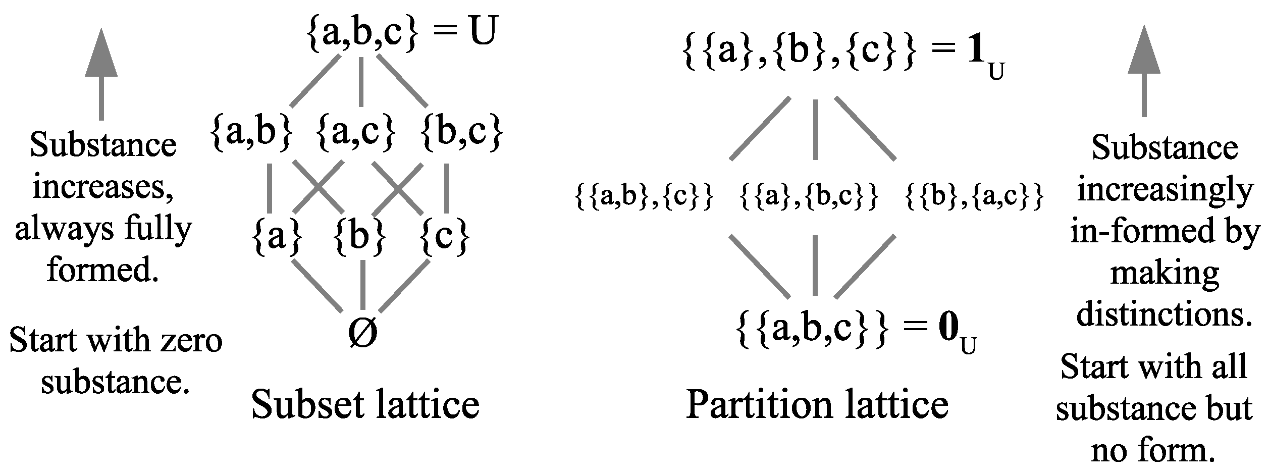
Figure 2.
Skeletonized quantum states of a particle as the lattice of partitions
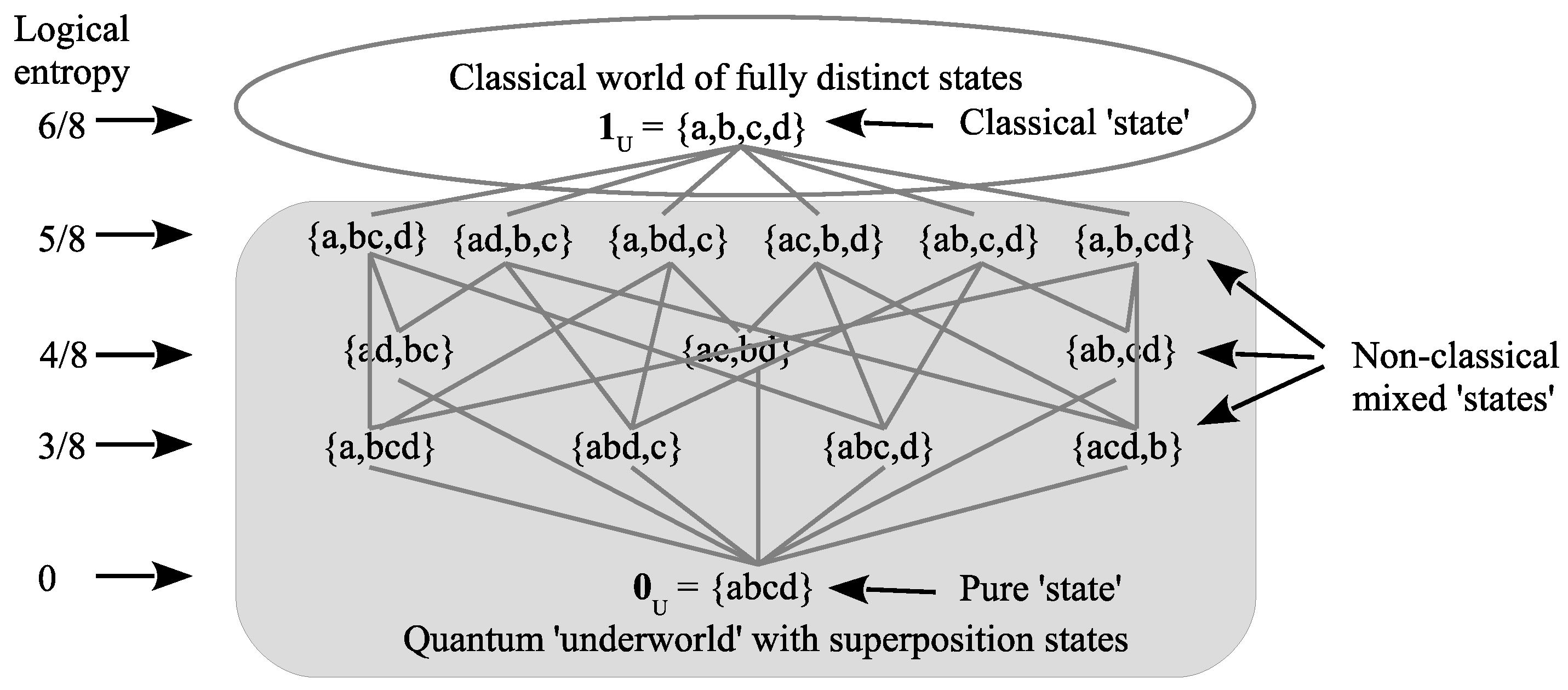
Figure 3.
`Wrong’ image of superposition in QM as sum of waves
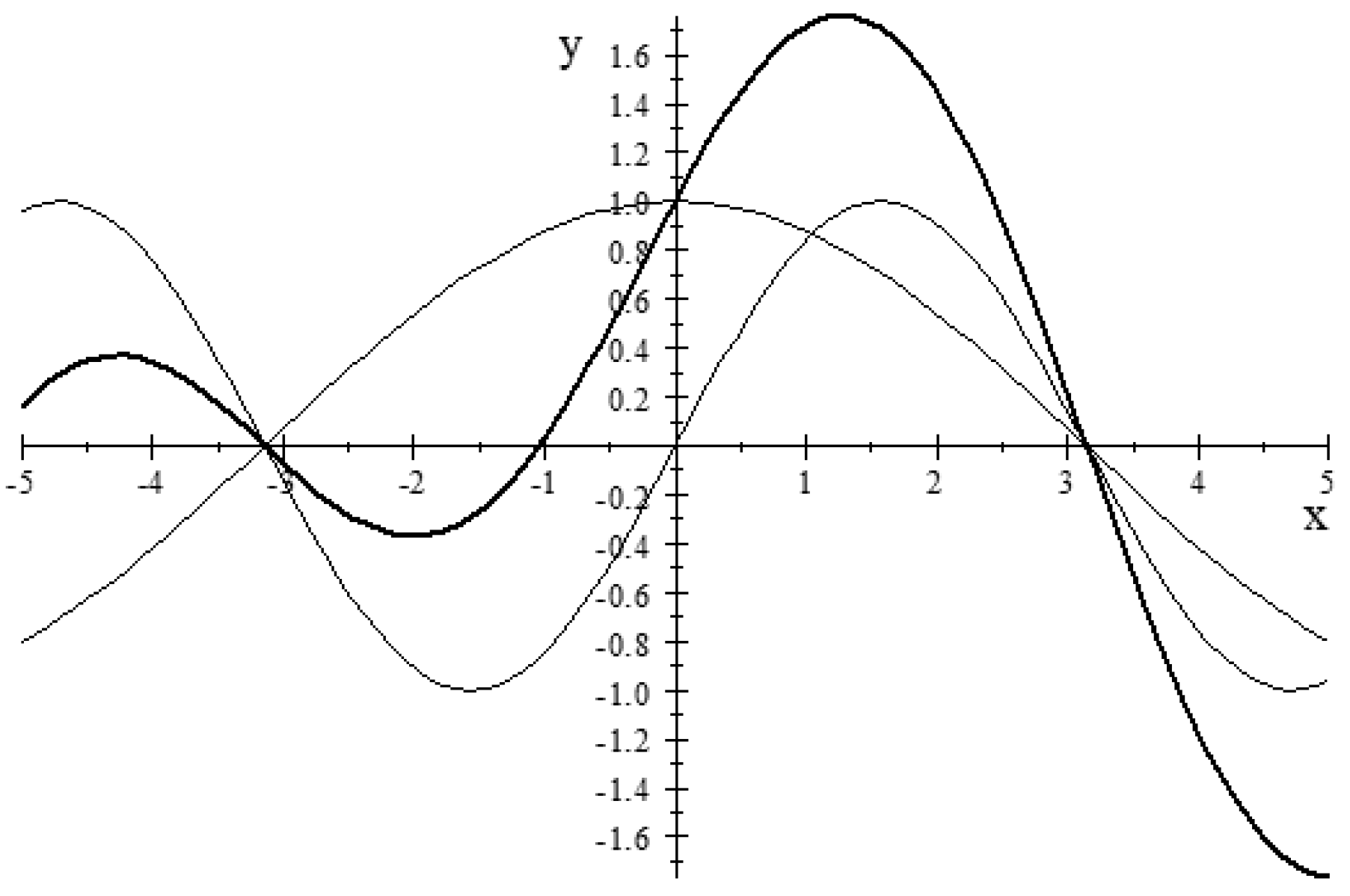
Figure 4.
Imagery of superposition as indefiniteness
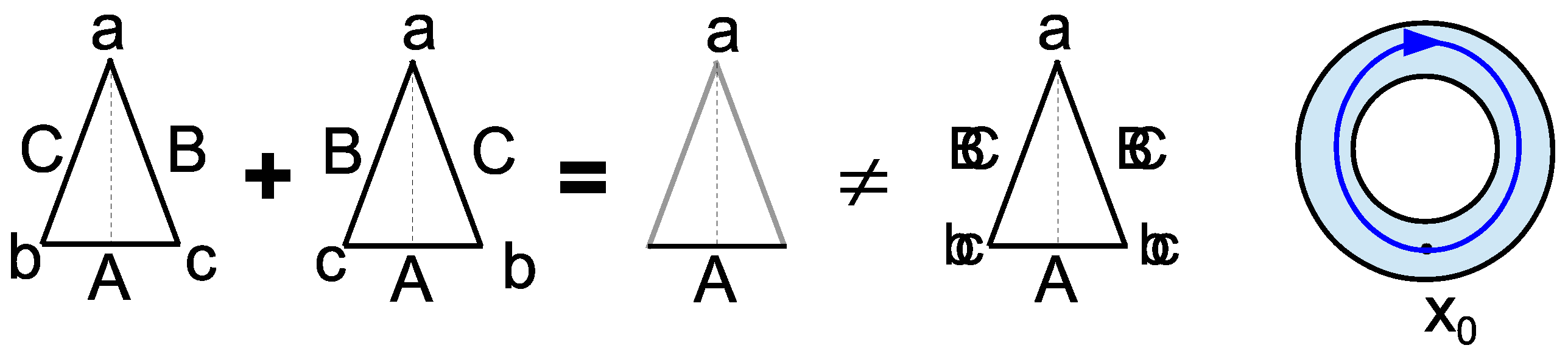
Figure 5.
Partition lattice with join
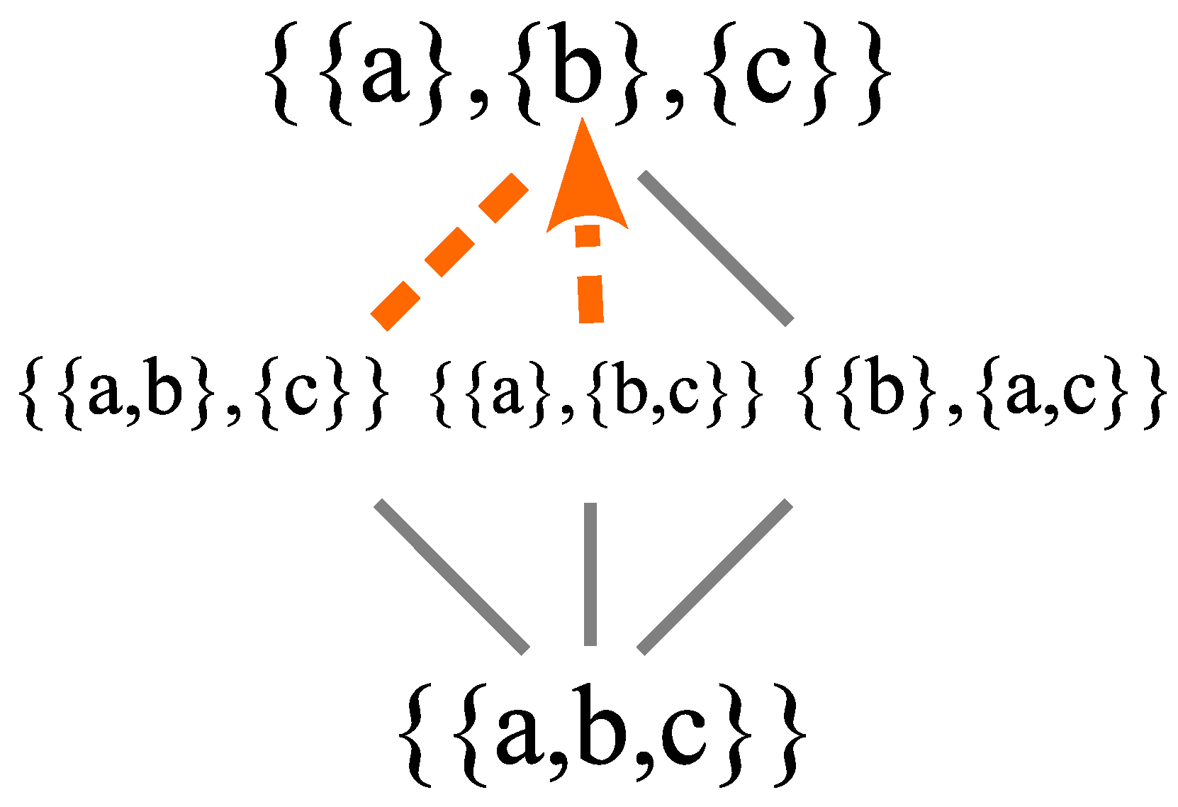
Figure 6.
Gratings imagery for Feynman’s rule distinguishable and indistinguishable alternatives
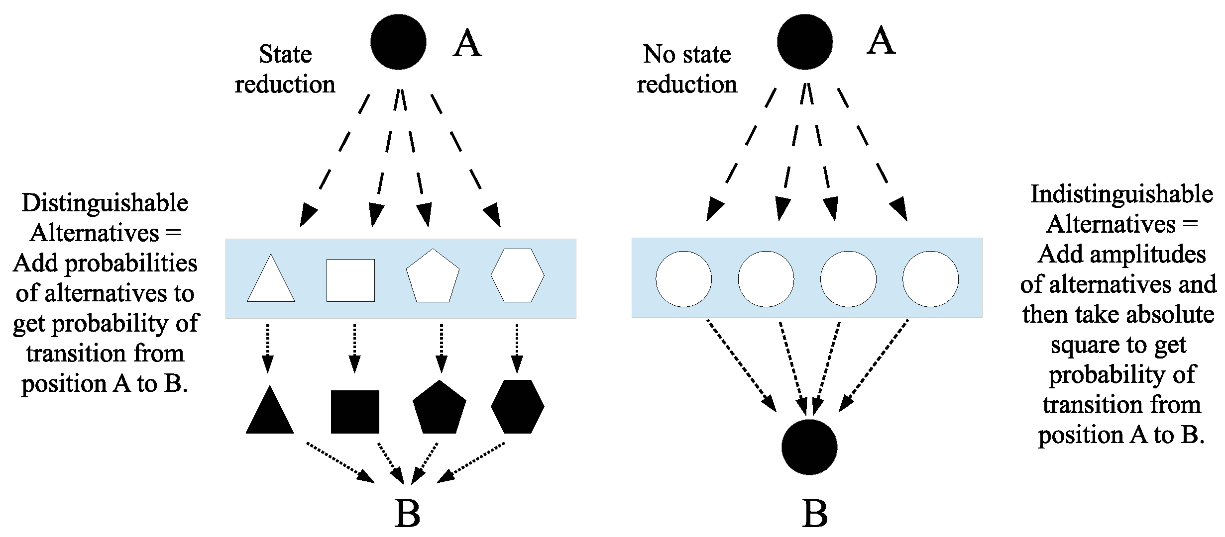
Figure 7.
Skeletal setup for the double-slit experiment
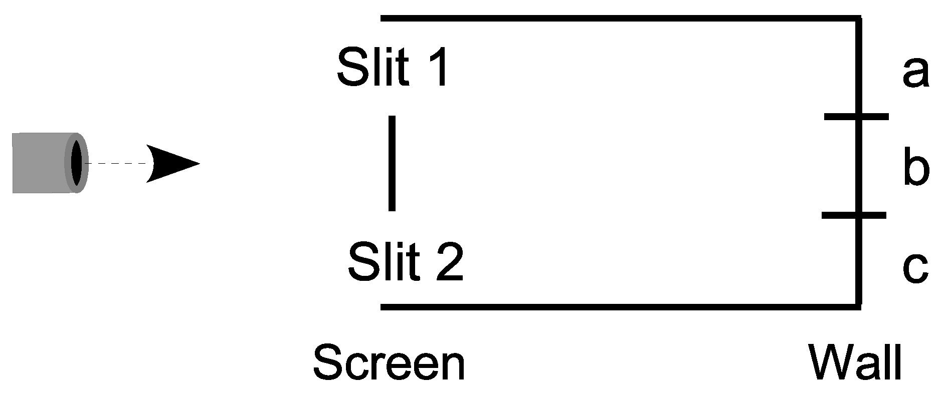
Figure 8.
Probabilities at the wall with distinctions at the screen
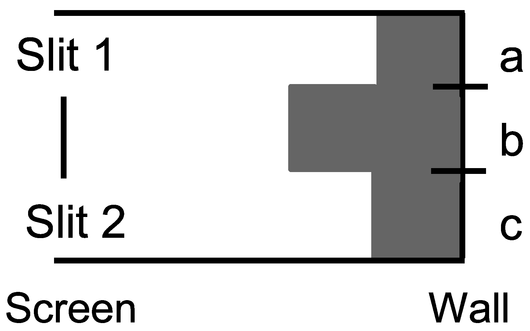
Figure 9.
Probabilities at the wall with no distinctions at the screen
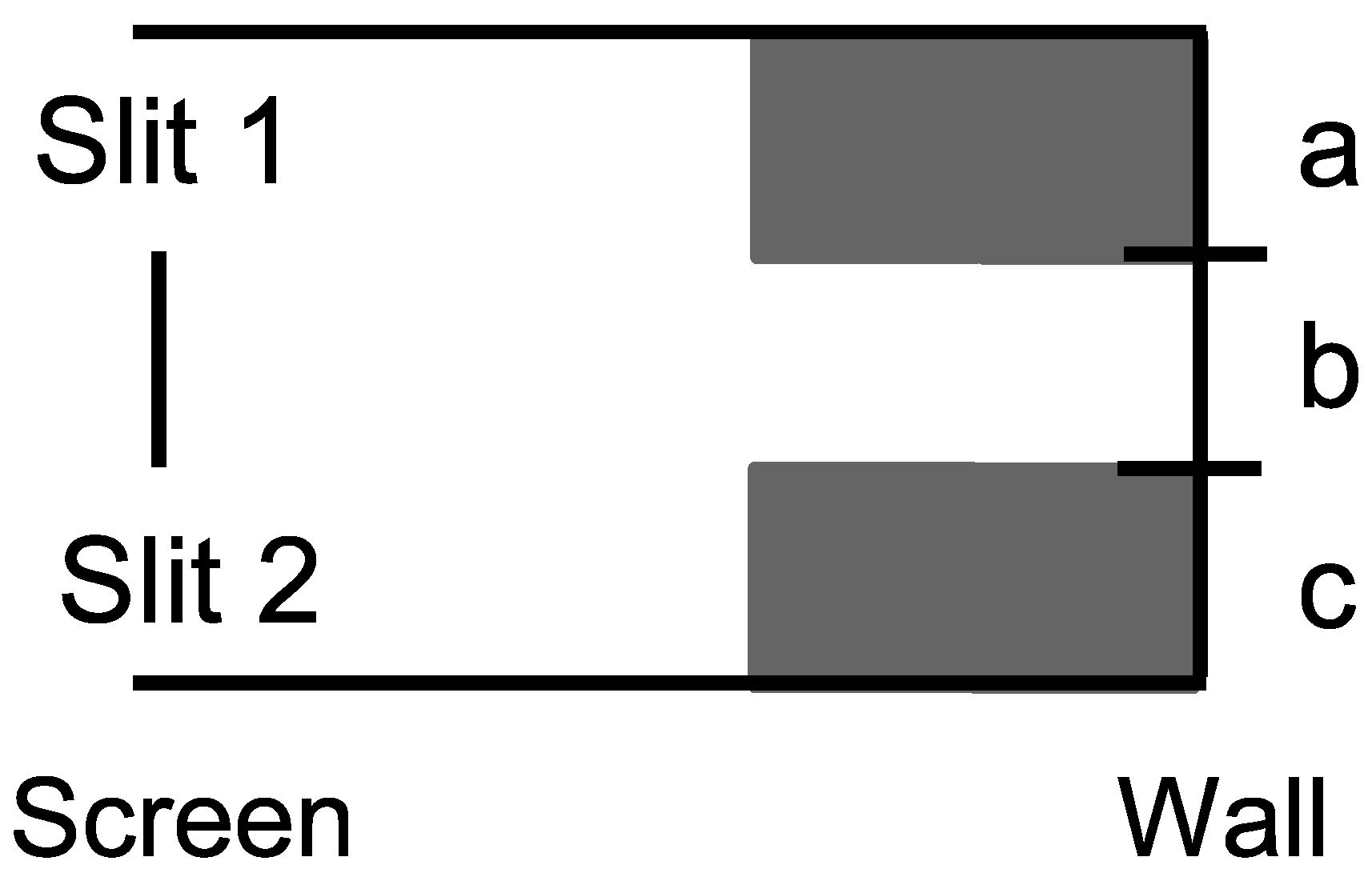
Figure 10.
Evolution taking place at a non-classical level of indefiniteness
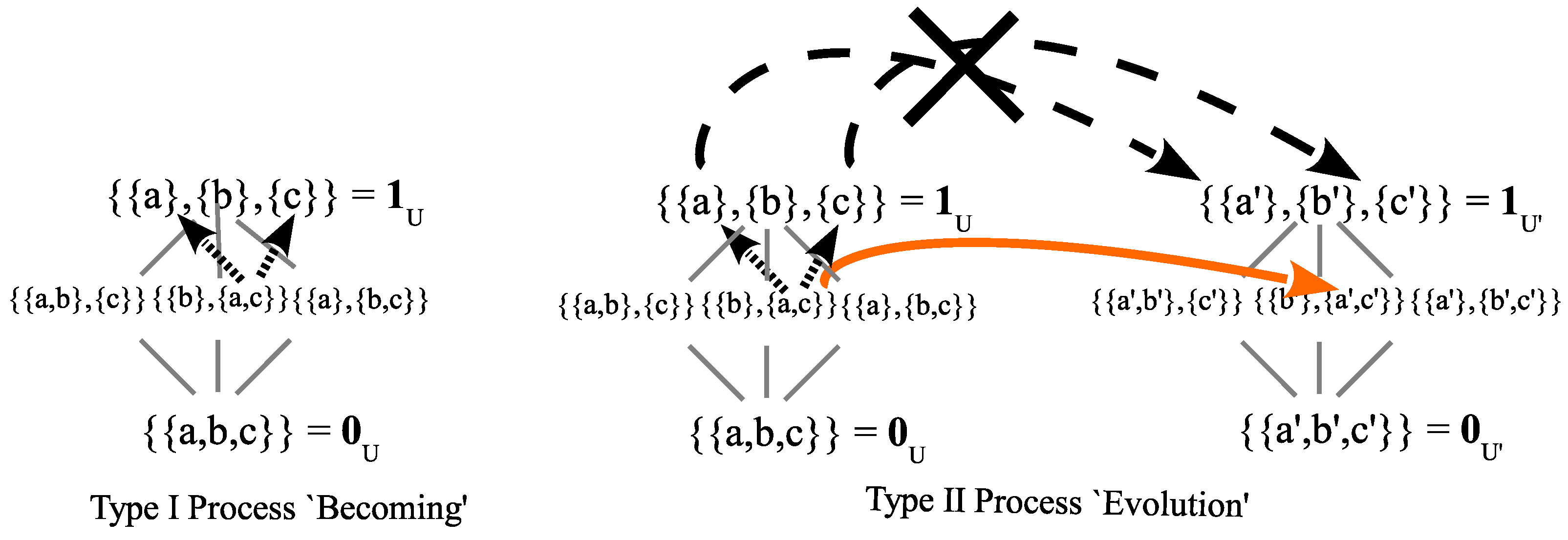
Figure 11.
Measurement at gates (owl has to walk from A to B through one of the gates)
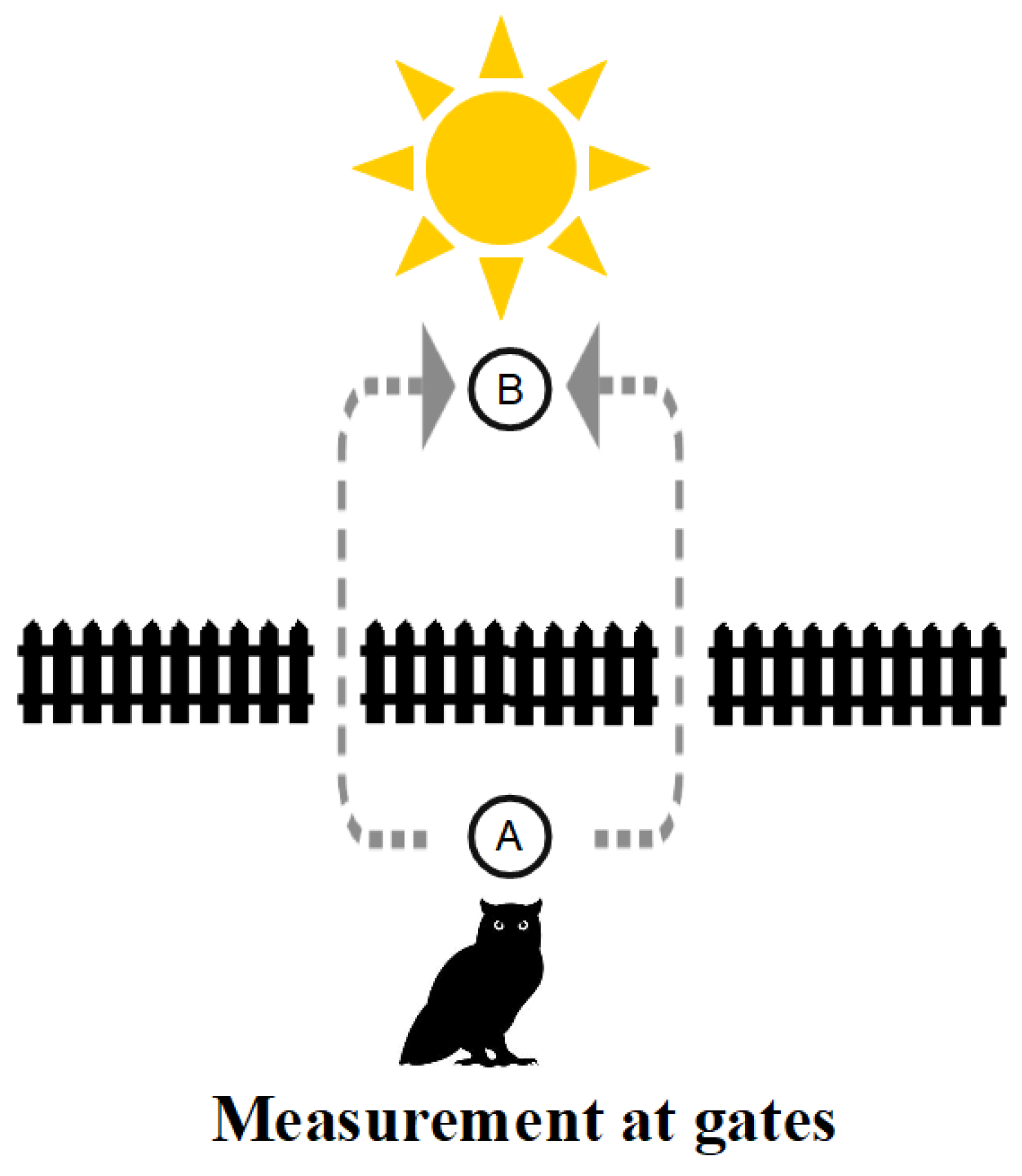
Figure 12.
No measurement at gates (owl can fly from A to B without going through a gate)
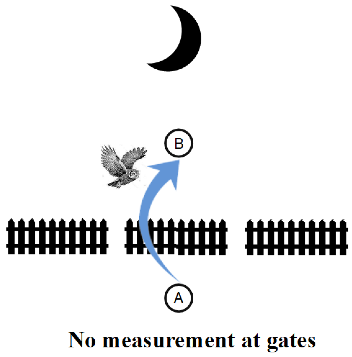

Table 1.
Elements and Distinctions (Its & Dits) duality between the two algebras.
| Algebra of subsets of U | Algebra of partitions on U |
|---|---|
| Its = Elements of subsets | Dits = Distinctions of partitions |
| P.O. Inclusion of subsets | P.O. Inclusion of ditsets |
| Join: | Join: |
| Top: Subset U with all elements | Top: Partition with all possible dits |
| Bottom: Subset ∅ with no elements | Bottom: Partition with no dits |
Table 2.
Set and Quantum versions of non-determinate and determinate results.
| Choice function | Quantum measurement (maximal) |
|---|---|
Table 3.
Corresponding partition and quantum concepts.
Table 4.
Quantum state as Hilbert space version of partition .
| Partition math | Hilbert space math |
|---|---|
| Density matrix: | |
| ON vectors: | |
| Eigenvalues: | |
| Spectral decomp.: | |
| Non-zero off-diagonals: Indistinction in a block | Coherence in a superposition |
Table 5.
Skeletal set-level concepts and the corresponding vector (Hilbert) space concepts.
Table 6.
Three basic notions: set version and corresponding Hilbert space version.
Disclaimer/Publisher’s Note: The statements, opinions and data contained in all publications are solely those of the individual author(s) and contributor(s) and not of MDPI and/or the editor(s). MDPI and/or the editor(s) disclaim responsibility for any injury to people or property resulting from any ideas, methods, instructions or products referred to in the content. |
© 2023 by the authors. Licensee MDPI, Basel, Switzerland. This article is an open access article distributed under the terms and conditions of the Creative Commons Attribution (CC BY) license (http://creativecommons.org/licenses/by/4.0/).
Copyright: This open access article is published under a Creative Commons CC BY 4.0 license, which permit the free download, distribution, and reuse, provided that the author and preprint are cited in any reuse.


