
Submitted:
13 December 2024
Posted:
17 December 2024
You are already at the latest version
Abstract
There is a fundamental duality that extends through the exact sciences. This paper briefly develops the relatively new logic of partitions dual to the Boolean logic of subsets. At a more basic level, the duality is between the elements of a subset and the distinctions (pairs of elements in different blocks) of a partition. Probability theory and information theory (based on logical entropy) start as the respective quantitative versions of the two dual logics of subsets and partitions. The subset side of the duality uses a one-sample (or one element) approach; the partition side uses a two-sample (or pair of elements) approach. The paper gives a new derivation of the variance and covariance based on that two-sample approach which positions those concepts on the partition and information-theory side of the duality.
Keywords:
fundamental subsets-partitions duality
; logic of subsets
; logic of partitions
; logical entropy
; variance
; covariance
1. Introduction: A Fundamental Duality in the Exact Sciences
A recent development in mathematical logic was the development of the logic of partitions (or equivalence relations) ([1,2,3]) that is category-theoretically dual to the usual Boolean logic of subsets. This initiated a series of developments, some new and some reformulations of older ideas, that showed how the duality extended throughout the mathematical sciences [4] (including quantum mechanics and beyond to the life sciences). The dual logics have quantitative versions. The quantitative version of subset logic is probability theory which is why George Boole’s book was entitled “An Investigation of the Laws of Thought on which are founded the Mathematical Theories of Logic and Probabilities”[5]. Gian-Carlo Rota conjectured on numerous occasions [6] that subsets are to probability as partitions are to information:
Accordingly, the quantitative version of partitions defined the notion of logical entropy which provides a logical foundation for the information theory ordinarily uses only the better-known notion of Shannon entropy.
There is a certain methodology used in developing this duality. That is, the notions associated with subset logic are defined in terms of single elements and the notions associated with partition logic are defined in terms of pairs of elements (or even ordered pairs). The simplest notion in mathematical statistics is the mean of a random variable (r.v.) which is associated with the single samplings of a random variable. The partition-motivated notion of a pair of samples of a r.v. turns out to be the logical basis for variance (and similarly covariance). This is not the usual definition of variance (or covariance) in the textbooks. It seems to be so little known that it has been announced as a new discovery [7], although that derivation of variance is much older [8] (p. 42) and was known as the variance formula that does not use the mean.
Our purpose here is to place that derivation of variance and covariance in the context of the fundamental category-theoretic duality starting with the dual logics of subsets and partitions. Moreover, this treatment of variance and covariance place those notions firmly on the information-theoretic side of the duality, not the probability-theoretic side. Hence we begin with the duality at the logical level.
2. Methods
2.1. The Duality of Subsets and Partitions
The mathematical logic that is currently presented in the form of “propositional” logic is really a special case of the Boolean logic of subsets.
The algebra of logic has its beginning in 1847, in the publications of Boole and De Morgan. This concerned itself at first with an algebra or calculus of classes, to which a similar algebra of relations was later added. Though it was foreshadowed in Boole’s treatment of `Secondary Propositions,’ a true propositional calculus perhaps first appeared from this point of view in the work of Hugh MacColl, beginning in 1877. [9] (pp. 155-56)
Category theory dates back to 1945 [10]. It provides a formal (turn around the arrows) notion of duality, and the dual of the notion of a subset is the notion of a quotient set or, equivalently, a partition or an equivalence relation. In general a subobject may be called a “part” and “The dual notion (obtained by reversing the arrows) of `part’ is the notion of partition.” [11] (p. 85)
This duality is missed when logic is only presented as “propositional” logic since propositions don’t have duals. Hence one needs the general Boolean notion of the logic of subsets to suggest a dual logic of partitions or equivalence relations. It was known in the 19th century (Richard Dedekind and Ernst Schröder) that partitions form a lattice with the operations of join ∨ and meet ∧. Gian-Carlo Rota and colleagues published a paper on the logic of certain equivalence relations but with only the lattice operations of join and meet and without any implication operation [12]. Indeed, no new operations of partitions or equivalence relations were developed in the 20th century.
Equivalence relations are so ubiquitous in everyday life that we often forget about their proactive existence. Much is still unknown about equivalence relations. Were this situation remedied, the theory of equivalence relations could initiate a chain reaction generating new insights and discoveries in many fields dependent upon it.
This paper springs from a simple acknowledgement: the only operations on the family of equivalence relations fully studied, understood and deployed are the binary join ∨ and meet ∧ operations. [13] (p. 445)
2.2. The Two Lattices of Subsets and of Partitions
A partition on a universe set () is set of non-empty subsets of U (called the blocks of the partition) that are disjoint and whose union is U. A distinction or dit of is an ordered pair of elements in distinct blocks of the partition . The set of distinctions or ditset is and its complement in is the set of indistinctions or indits which is just the equivalence relation version of the partition where the blocks of the partition are the equivalence classes of the equivalence relation.
In the Boolean lattice of subsets , the join is the union of subsets, the meet is the intersection, and the partial order is the inclusion relation between subsets. The implication or conditional operation on subsets of U is denoted and is defined as (where is the complement of S). The addition of the conditional operation turns the Boolean lattice into the Boolean algebra of subsets.
Partitions on U also form a lattice, the partition lattice . Given and partitions on U, the join is the partition on U whose blocks are the non-empty intersections for and . The ditset of the join is just the union of the ditsets, i.e., . Since the join in the lattice of subsets is just the union of the elements of the two subsets , we see that the distinctions or “Dits” of a partition play the corresponding role as the elements or “Its” of a subset in the duality between subsets and partition.
To define the meet of two partitions, suppose that if two blocks and overlap (i.e., the intersection is non-empty) then they unite like two blobs of mercury, i.e., take their union . Doing this for all overlaps, we eventually arrive as subsets that are the exact union of blocks of and also the exact union of blocks of and are minimal in that regard. Those are the blocks of the meet .
The new implication operation partitions, denoted , is defined as the partition that is like except when a block is contained in some block , i.e., , then is replaced by its discretization, i.e., by the singleton blocks of its elements.
The partial order for partitions is called refinement where refines , written , if for every block , there is a block of such that . Intuitively, can be obtained from by chopping up some blocks of . Some older texts ([14,15]) define the “lattice of partitions” with the reverse partial order (which reverses the join and meet) which Gian-Carlo Rota called “unrefinement” or “reverse refinement” [6] (p. 30). With the refinement partial order, refinement is just the inclusion of distinctions, i.e., if and only if , just as the partial order in the Boolean lattice is inclusion of elements. That is one way the dual connection between “elements” and “distinctions” shows itself. The top of the lattice of partitions is the discrete partition where all blocks are singletons and the bottom is the indiscrete partition where the only block is U. The addition of the implication operation turns the (19th century) notion of a partition lattice into the (21st century) notion of a partition algebra.
When the respective implications are equal to the top element, then and only then the partial order relation holds, i.e.,
iff
iff .
For , the two lattices are illustrated in Figure 1.
Table 1 summarizes the duality between the lattice of subsets and the lattice of partitions .
Hence we can extend Rota’s duality statement to that between elements of subsets and distinctions of partitions:
.
One aspect of the dual concepts of elements and distinctions (that we will employ later), is that elements are a one-variable concept while distinctions are pairs of elements. The basic questions about elements are, for instance, does a predicate apply to it or not which is a question about existence, i.e., does it exist in the subset of elements with that property or not. The basic questions about distinctions are about, given two elements, are they distinct or not in the partition or are they equivalent or not in the corresponding equivalence relation. As we will see, this duality between single-element concepts and pair-concepts comes out in statistics.
2.3. Fundamental Status of the Two Lattices
The notions of a subset of a set and a partition on a set are defined without any additional structure on the sets. Hence the lattices, algebras, and logics of those two notions have a certain fundamental status. Given a topology or a partial order on a set, then other lattices can be defined in terms of that additional structure. But the notions of subsets and partitions require no such additional structure and thus their fundamentality. Moreover, subsets and partitions are category-theoretically dual concepts.
The two dual logics provide a modern model for the old Aristotelian duality of substance versus form(as in in-form-ation) [16]. We can tell two abstract “creation stories” by moving up in the two lattices from the bottom to the top. We see that the existence of substance increases in the subset lattice while form stays constant (always classical in the sense of being fully distinct), and the reverse happens in the partition lattice.
For each lattice where , start at the bottom and move towards the top in Figure 2.
There is no substance or “Its” (elements) at the bottom ∅ of the subset lattice, and as one moves up, new “Its” or elements appear but always fully formed, i.e., no indefiniteness, until one reaches the full universe U. At the bottom of the partition lattice, there are no dits (distinctions), i.e., , and all the substance already appears but with no form (i.e., no “Dits” in just as no “Its” in ∅). As one moves up the lattice of partitions, form (as in in-form-ation) is created by making new dits or distinctions until reaching the partition that makes all possible distinctions, i.e., where is the diagonal of all the self-pairs of elements of U, since an element cannot be distinguished from itself.
The progress from bottom to top of the two lattices can be described as two creation stories.
- Subset creation story: “In the Beginning was the Void”, and then elements are created, fully propertied and distinguished from one another, until finally reaching all the elements of the universe set U.
- Partition creation story: “In the Beginning was undifferentiated Substance (e.g., “Formless Chaos”), and then there is a “Big Bang” where the substance is being objectively in-formed by the making of distinctions (i.e., symmetry-breaking) until the result is finally the singletons which designate the elements of the universe U.
Heisenberg identifies “substance” with energy.
Energy is in fact the substance from which all elementary particles, all atoms and therefore all things are made, and energy is that which moves. Energy is a substance, since its total amount does not change, and the elementary particles can actually be made from this substance as is seen in many experiments on the creation of elementary particles [17] (p. 63).
Thus the partition creation story, can be viewed as a bare-bones description of the Big Bang theory of creation–constant substance (energy) in-formed by symmetry-breaking distinctions [18].
2.4. Logical Entropy
2.4.1. A Little History of Information-As-Distinctions
When the logic of partitions was developed [3], then it could imitate Boole’s development of logical probability as the quantitative version of subsets [5]. Logical probability was the number of elements in a subset normalized by the cardinality of U. The dual to the notion of an element of a subset is a distinction of a partition.
The wide-ranging anthropologist, Gregory Bateson, described information as “differences that make a difference.” [19] (p. 99). One of the founders of quantum information theory, Charles Bennett, has described information as “the notion of distinguishability abstracted away from what we are distinguishing, or from the carrier of information... .” [20] (p. 155). But the notion of information as the quantification of distinctions or differences goes back almost four centuries. In The Information: A History, A Theory, A Flood by James Gleick, he noted the focus on distinctions or differences in the 17th century polymath and founder of the Royal Society, John Wilkins. In 1641, the year before Newton was born, Wilkins published one of the earliest books on cryptography, Mercury or the Secret and Swift Messenger, which not only pointed out the fundamental role of differences but noted that any (finite) set of different things could be encoded by words in a binary code.
For in the general we must note, that whatever is capable of a competent difference, perceptible to any sense, may be a sufficient means whereby to express the cogitations. It is more convenient, indeed, that these differences should be of as great variety as the letters of the alphabet ; but it is sufficient if they be but twofold, because two alone may, with somewhat more labour and time, be well enough contrived to express all the rest [21] (p. 67).
Wilkins explains that a five letter binary code would be sufficient to code the letters of the alphabet since .
Thus any two letters or numbers, suppose A. B. being transposed through five places, will yield thirty-two differences, and so consequently will superabundantly serve for the four and twenty letters,... [21] (pp. 67-8).
As Gleick noted:
Any difference meant a binary choice. Any binary choice began the expressing of cogitations. Here, in this arcane and anonymous treatise of 1641, the essential idea of information theory poked to the surface of human thought, saw its shadow, and disappeared again for [three] hundred years [22] (p. 161).1
Gleick is here dating the development of modern information theory from Claude Shannon’s work published in 1948 [25]. This is how the development of the logic of partitions, dual to the Boolean logic of subsets, and using the duality between the elements-of-a-subset (or Its) and the distinctions-of-a-partition (or Dits), reveals a dual relationship between logical probability theory and logical information theory.
2.4.2. The Mathematics of Logical Entropy
We have seen how probability theory starts with the notion of logical probability of a subset (or event) as the normalized number of elements in the subset S:
.
We have also seen the duality between subsets and partitions expressed as:
and
which also means that:
.
Hence the logical notion of information in a partition should be the normalized number of distinctions in the partition. Following Shannon’s labeling of his quantification of information as “entropy,” we will call the notion based on quantifying the logic of partitions as “logical entropy.” ([23,24]) For a partition , the logical entropy of is the normalized number of distinctions:
where the product version of the formula follows from:
.
As in the case of logical probability, we are, for the moment, assuming equiprobable points in U. Moreover, it should be noted that for probability, we are dealing with single samples and for information, we are dealing with pairs, indeed ordered pairs of elements drawn from U so that each pair of distinct blocks and is counted twice in the sum . This yields an immediate simple interpretation of logical entropy, namely that is the probability that in two independent samples from U, one obtains a distinction of .
The formulas generalize immediately to the general case of finite probability theory where the points of U have the respective point probabilities of . Then and
When the given data is just the probability distribution p on U, then
which could also be viewed as the logical entropy of the discrete partition , i.e., . In all the cases, the logical entropy is the two-sample probability of getting a distinction. The least value of logical entropy is 0 for the indiscrete partition or for p where some . The maximum value for logical entropy is for the discrete partition with equiprobable points:
which is interpreted simply as the probability that the second draw from U will be different from the first draw.
Diagrammatically, the logical entropy is illustrated using a box diagram with a unit square. For instance for , the box diagram is given in Figure 3 where each of the halves is:
.
Since the logical entropy of a partition has a probability interpretation, it is can be obtained as the value of a subset on a probability measure. The probability measure is the product measure on the set and the subset giving the logical entropy is , i.e.,
.
Since , which is sometimes written as as the joint entropy. There is a natural closure operation on subsets , namely the reflexive-symmetric-transitive (RST) closure of S which is the smallest indit set or equivalence relation containing S so its complementary ditset will define a partition. Although they are the complements of a set under a closure operation, ditsets are not like the open sets in a topological space and the RST closure is not a topological closure operation. The arbitrary union of ditsets is a ditset but the intersection of ditsets is not necessarily a ditset (unlike open sets). But that intersection is nevertheless a subset of so its probability measure defines the mutual information: . Similarly, the difference information is: which is interpreted as the information in that is not in . Then we have the usual Venn diagram relationships illustrated in Figure 4:
.
2.4.3. The Relationship with Shannon Entropy
The well-known Shannon entropy [25], , is not defined as the values of certain subsets of a measure on a set. Shannon defined his notions of joint, mutual, and difference or conditional entropy directly in terms of probabilities and defined them so that the Venn diagrams relationships nevertheless held.
Andrei Kolmogorov objected to Shannon defining information directly in terms of probabilities and instead thought it should be based on a prior combinatorial structure.
Information theory must precede probability theory, and not be based on it. By the very essence of this discipline, the foundations of information theory have a finite combinatorial character [26] (p. 39).
Kolmogorov had his own ideas but it might be noticed that the logical entropy definition of information-as-distinctions is based on probability-free sets of a combinatorial nature, namely, ditsets.
The fact that the compound notions of Shannon entropy satisfy the Venn diagram relations, in spite of not being defined as a measure in the sense of measure theory, is explained by the fact that logical entropy is defined as a measure and there is a uniform transformation between the compound logical entropy and Shannon entropy formulas that preserves Venn diagrams. This raises the question of that relationship between the two entropies.
If an outcome has probability close to or equal to 1, then the occurrence of that outcome intuitively gives little or no information. Therefore, it might be said that information is related to the complement of 1–but there are two complements to 1, the additive complement and the multiplicative complement . The additive and multiplicative averages of the respective 1-complements give the two entropies. The additive probabilistic average of the additive 1-complements is the logical entropy: . The multiplicative average of the multiplicative 1-complements is the Shannon entropy in its log-free or anti-log form: . One chooses the particular log for the context, e.g., for coding theory or natural logs for statistical mechanics. Since the log of the multiplicative average transforms it to an additive average, the two additive averages can be transformed, one into the other, by the dit-bit transform . Once the compound formulas are expressed in terms of the additive 1-complements, then this non-linear but monotonic dit-bit transform yields the corresponding compound formulas for Shannon entropy [23]. And the dit-bit transform preserves Venn diagrams.
2.4.4. Some History of the Logical Entropy Formula
The formula for logical entropy is not new; it is only the derivation as the quantitative version of the new partition logic that is new. The formula goes back at least to 1912 in the index of mutability of Corrado Gini [27]. The formula resurfaced in the coding-breaking activity in World War II ([28,29]) where it was the additive 1-complement of Alan Turing’s repeat rate where it became part of the mathematics of cryptography [30]. After the war, Edmund Simpson published the formula as a quantification of biodiversity [31]. Hence the formula is often know as the Gini-Simpson formula for biodiversity [32]. But Simpson along with I. J. Good worked with Turing at Bletchley Park during WWII, and, according to Good, “E. H. Simpson and I both obtained the notion [the repeat rate] from Turing.” [28] (p. 395) When Simpson published the index in 1948, he (again, according to Good) did not acknowledge Turing “fearing that to acknowledge him would be regarded as a breach of security” [33] (p. 562).
Two elements from are either identical or distinct. Gini [27] introduced as the “distance” between the and elements where for and , i.e., , the complement to the Kronecker delta. Since , the logical entropy, i.e., Gini’s index of mutability, , is the average logical distance between a pair of independently drawn elements. In 1982, C. R. (Calyampudi Radhakrishna) Rao generalized this by allowing other non-negative distances for (but always ) between the elements of U so that would be the average distance between a pair of independently drawn elements from U which was know as quadratic entropy [34].
3. Results: The Logical Basis for Variance and Covariance
At the logical level, the fundamental duality starts with the duality between the Boolean logic of subsets and the logic of partitions. At a more granular level, it is the duality between elements (Its) of a subset and distinctions (Dits) of a partition. The elements of a subsets are certain singular elements from the universe set and the distinctions of a partition are certain pairs (or ordered pairs) of elements of the universe set.
Given with the probability distribution , consider a real-valued random variable (r.v.) . The inverse-image defines a partition on U where the values in the image of the r.v. are . Then each value has the probability: .
On the one (single-values) side of the duality, the probability average of the single values is the usual mean: . But what is the appropriate notion on the other (pair-of-values) side of the duality?
In the same 1912 book [27] where Gini suggested the index of mutability of a probability distribution, he suggested the mean difference . Maurice Kendall noted that the mean difference “has a certain theoretical attraction, being dependent on the spread of the variate-values among themselves and not on the deviations from some central value.” [8] (p. 42) But Kendall went on to note: “It is, however, more difficult to compute than the standard deviation, and the appearance of the absolute values in the defining equations indicates, as for the mean deviation, the appearance of difficulties in the theory of sampling.” [8] (p. 42) At a later date, Kendall summarized his criticism; the mean difference (in comparison to the variance) lacked “ease of calculation, mathematical tractability and sampling simplicity.” [35] (p. 223)
Kendall noted that if one tried to improve the mean difference formula by using the square of the difference in values, then that “is nothing but twice the variance” [8] (p. 42) since:
.
This means the C. R. Rao’s quadratic entropy for the distance function is twice the variance. We noted previously that the consideration of pairs could take the form of just pairs or ordered pairs (where ) . Hence the variance may be defined using just simple pairs:
This interesting relation shows that the variance may in fact be defined as half the mean square of all possible variate differences, that is to say, without reference to deviations from a central value, the mean. [8] (p. 42)
The “interesting relation” also extends to the covariance. Suppose there are two random variables X with values for and Y with values for with probabilities given by a joint distribution . The two samples or two draws methodology gives two ordered pairs and so the double-variance formula generalizes to:
which is similarly equal to twice the covariance .
Since if or , we can sum over all . Abbreviating , we have:
.
Then using:
, and
and similarly for the other cases, we have:
.
Using the lexicographical ordering of the ordered pairs of indices (i.e., ordering according to first index, or if , then according to the second index), we have:
.
4. Discussion and Conclusions
These results shed new light on the variance in terms of the fundamental duality that starts in the two dual logics of subsets and partitions, and extends throughout the exact sciences [4]. The aspects discussed in this paper are given in Table 2.
We see the one-draw methodology in the notion of the probability of a subset (the one-draw-from-U probability of getting an element of a subset S) and the two-draw methodology in the notion of the logical entropy of a partition (the two-draw-from-U probability of getting a distinction of a partition ). Applied to a random variable , the one-draw method gives the mean and the two-draw method gives the variance.
The quantitative versions of the two logics associates the one-draw method with probability theory and the two-draw method with information theory–which implies that the variance should be seen as an information-theoretic concept. The usual definition of the variance gives no hint of the two-draw approach. The Shannon entropy is often taken as a quantification of uncertainty with some integration into statistical theory ([36,37] (Chap. 11)). But the much older notion of uncertainty in statistical theory is the variance. The logical entropy is the two-draw probability of the distinctions of a partition and the variance is the two-draw probability of the square of the value-distinctions of a random variable (and similarly for the covariance). That is the new logical basis for variance and covariance that positions those concepts on the partitions/information-theory side of the fundamental subsets-partitions duality.
Funding
This research received no external funding.
Conflicts of Interest
The author declares no conflicts of interest.
Abbreviations
| RST | Reflexive-Symmetric-Transitive |
References
- Ellerman, David 2010. The Logic of Partitions: Introduction to the Dual of the Logic of Subsets. Review of Symbolic Logic. 3 (2 June): 287-350.
- Ellerman, David. 2014. An Introduction of Partition Logic. Logic Journal of the IGPL. 22 (1): 94–125.
- Ellerman, David. 2023. The Logic of Partitions: With Two Major Applications. Studies in Logic 101. London: College Publications. https://www.collegepublications.co.uk/logic/?00052.
- Ellerman, David. 2024. “A Fundamental Duality in the Exact Sciences: The Application to Quantum Mechanics.” Foundations 4 (2): 175–204. [CrossRef]
- Boole, George 1854. An Investigation of the Laws of Thought on which are founded the Mathematical Theories of Logic and Probabilities. Cambridge: Macmillan and Co.
- Kung, Joseph P. S., Gian-Carlo Rota and Catherine H. Yan 2009. Combinatorics: The Rota Way. New York: Cambridge University Press.
- Zhang, Yuli, Huaiyu Wu, and Lei Cheng. 2012. “Some New Deformation Formulas about Variance and Covariance.” In Proceedings of 2012 International Conference on Modelling, Identification and Control (ICMIC2012), 987–92.
- Kendall, M. G. 1945. Advanced Theory of Statistics Vol. I. London: Charles Griffin & Co.
- Church, Alonzo 1956. Introduction to Mathematical Logic. Princeton: Princeton University Press.
- Eilenberg, Samuel and Saunders Mac Lane. 1945. General Theory of Natural Equivalences. Transactions of the American Mathematical Society. 58, No2, 231-94.
- Lawvere, F. William and Robert Rosebrugh 2003. Sets for Mathematics. Cambridge: Cambridge University Press.
- Finberg, David, Matteo Mainetti and Gian-Carlo Rota 1996. The Logic of Commuting Equivalence Relations. In Logic and Algebra. Aldo Ursini and Paolo Agliano ed., New York: Marcel Dekker: 69-96.
- Britz, Thomas, Matteo Mainetti and Luigi Pezzoli 2001. Some operations on the family of equivalence relations. In Algebraic Combinatorics and Computer Science: A Tribute to Gian-Carlo Rota. H. Crapo and D. Senato eds., Milano: Springer: 445-59.
- Birkhoff, Garrett 1948. Lattice Theory. New York: American Mathematical Society.
- Grätzer, George 2003. General Lattice Theory (2nd ed.). Boston: Birkhäuser Verlag.
- Ainsworth, Thomas. 2016. Form vs. Matter. In The Stanford Encyclopedia of Philosophy (Spring 2016 Edition), edited by Edward N. Zalta. https://plato.stanford.edu/archives/spr2016/entries/form-matter/.
- Heisenberg, Werner 1958. Physics & Philosophy: The Revolution in Modern Science. New York: Harper Torchbooks.
- Pagels, Heinz. 1985. Perfect Symmetry: The Search for the Beginning of Time. New York: Simon and Schuster.
- Bateson, Gregory. 1979. Mind and Nature: A Necessary Unity. New York: Dutton.
- Bennett, Charles H. 2003. “Quantum Information: Qubits and Quantum Error Correction.” International Journal of Theoretical Physics 42 (2 February): 153–76. [CrossRef]
- Wilkins, John. 1802. Mercury: or the Secret and Swift Messenger. In The Mathematical and Philosophical Works of the Right Rev. John Wilkins, Vol. II. London: C. Whittingham:1–87.
- Gleick, James 2011. The Information: A History, A Theory, A Flood. New York: Pantheon.
- Ellerman, David. 2021. New Foundations for Information Theory: Logical Entropy and Shannon Entropy. Cham, Switzerland: SpringerNature. [CrossRef]
- Manfredi, Giovanni. 2022. “Logical Entropy – Special Issue.” 4Open, no. 5: E1. [CrossRef]
- Shannon, Claude E. 1948. A Mathematical Theory of Communication. Bell System Technical Journal. 27: 379-423.
- Kolmogorov, Andrei N. 1983. Combinatorial Foundations of Information Theory and the Calculus of Probabilities. Russian Math. Surveys 38 (4): 29–40.
- Gini, Corrado 1912. Variabilità e mutabilità. Bologna: Tipografia di Paolo Cuppini.
- Good, I. J. 1979. A.M. Turing’s statistical work in World War II. Biometrika. 66 (2): 393-6.
- Rejewski, M. 1981. How Polish Mathematicians Deciphered the Enigma. Annals of the History of Computing. 3: 213-34.
- Kullback, Solomon 1976. Statistical Methods in Cryptoanalysis. Walnut Creek CA: Aegean Park Press.
- Simpson, Edward Hugh 1949. Measurement of Diversity. Nature. 163: 688.
- Rao, C. R. 1982. “Gini-Simpson Index of Diversity: A Characterization, Generalization and Applications.” Utilitas Mathematica B 21: 273–82. 623-56.
- Good, I. J. 1982. Comment (on Patil and Taillie: Diversity as a Concept and its Measurement). Journal of the American Statistical Association. 77 (379): 561-3.
- Rao, C. Radhakrishna 1982. Diversity and Dissimilarity Coefficients: A Unified Approach. Theoretical Population Biology. 21: 24-43.
- Kendall, M. G. 1957. “Review of Variabilita e Concentrazione. By Corrado Gini.” Journal of the Royal Statistical Society. Series A (General) 120 (2): 222–23.
- Kullback, Solomon. 1968. Information Theory and Statistics. New York: Dover.
- Cover, Thomas, and Joy Thomas. 2006. Elements of Information Theory. Second Ed. Hoboken NJ: John Wiley and Sons.
| 1 | An old Pennsylvania Dutch superstition is that if on the second of February each year, a groundhog emerges from its den and sees its shadow, then it stays in its den for another six weeks. |
Figure 1.
Lattices of subsets and of partitions.
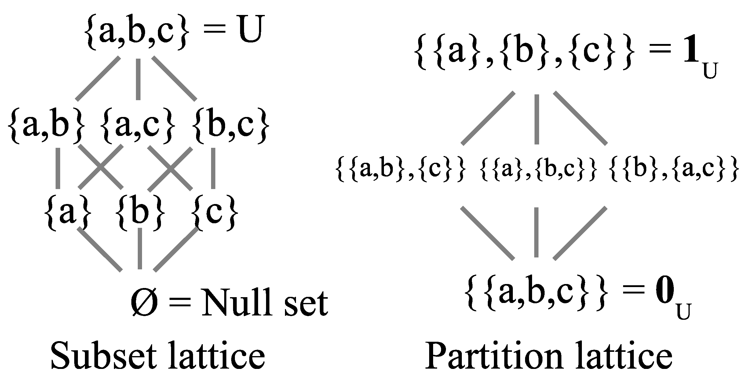
Figure 2.
Moving up the subset and partition lattices.
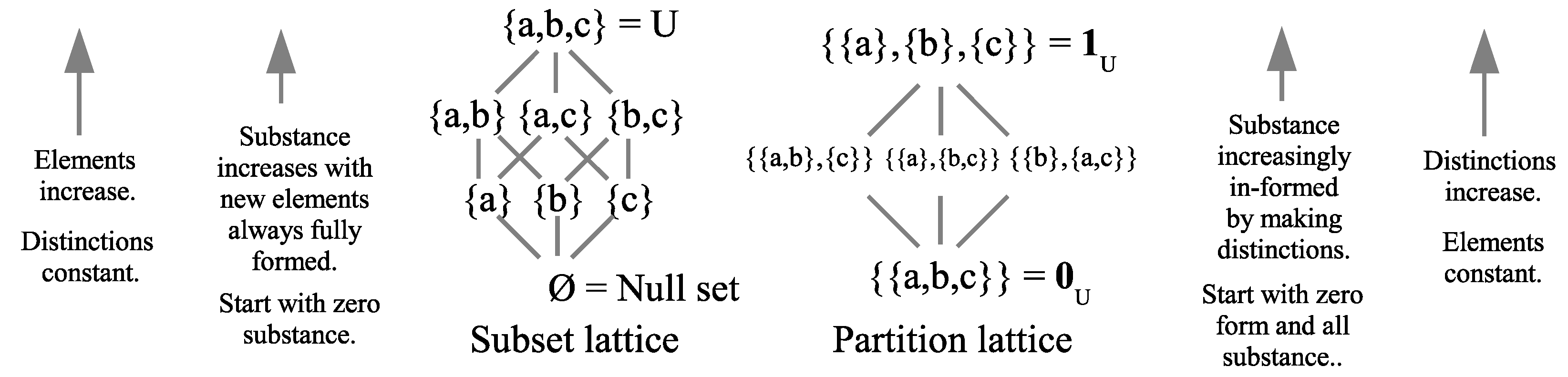
Figure 3.
Logical entropy box diagram.
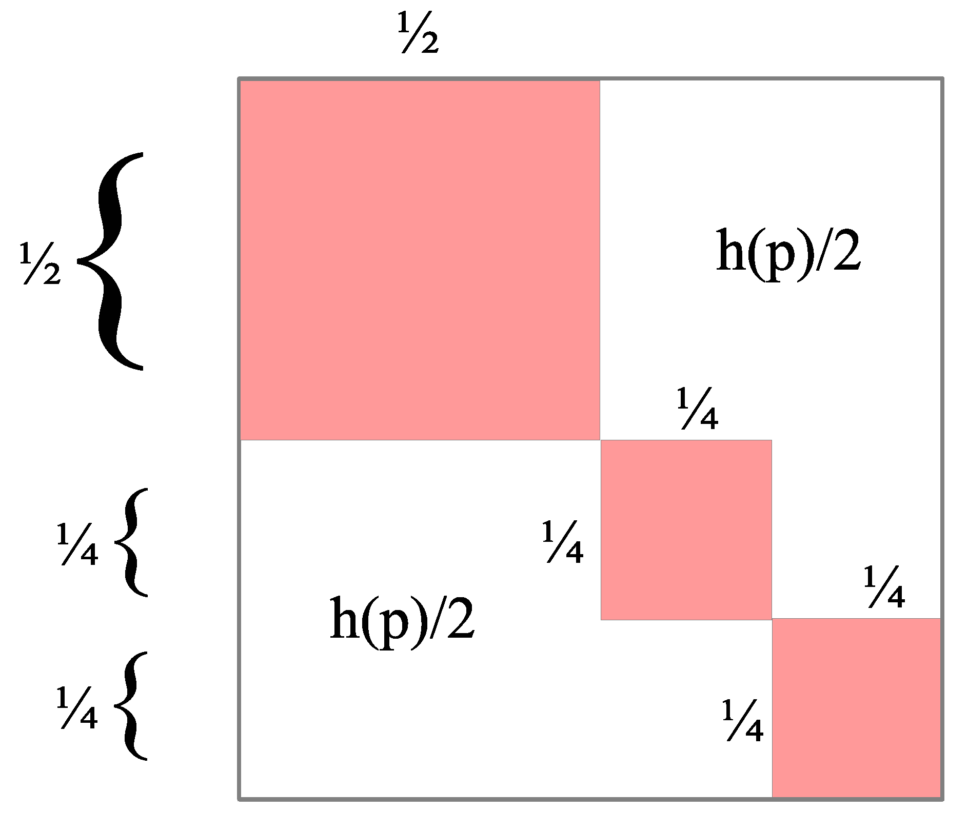
Figure 4.
Venn diagram relationships for logical entropy.
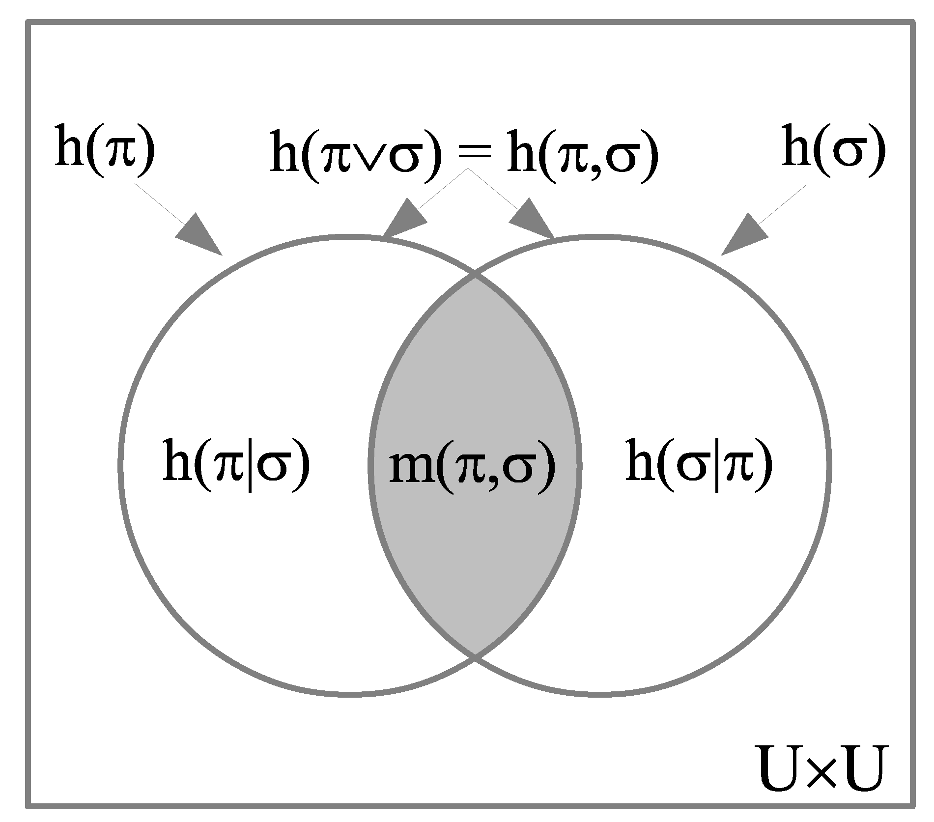

Table 1.
Elements-distinctions duality between the two dual lattices.
| Dualities | Boolean lattice of subsets | Lattice of partitions |
| “Its” or “Dits” | Elements of subsets | Distinctions of partitions |
| Partial order | ||
| Join | ||
| Top | Subset U with all elements | Partition with all distinctions |
| Bottom | Subset ∅ with no elements | Partition with no distinctions |
Table 2.
Parts of the fundamental duality discussed here.
| Fundamental Duality | Subset or Its side | Partition or Dits side |
|---|---|---|
| Its & Dits | Elements of subsets | Distinctions of partitions |
| Logic | Subset logic | Partition logic |
| “Creation stories” | Ex Nihilo | Big Bang |
| Quantitative versions | Probability | Logical entropy |
| Sampling | 1-draw | 2-draw (with replacement) |
| Random variable X | Mean | Variance |
Disclaimer/Publisher’s Note: The statements, opinions and data contained in all publications are solely those of the individual author(s) and contributor(s) and not of MDPI and/or the editor(s). MDPI and/or the editor(s) disclaim responsibility for any injury to people or property resulting from any ideas, methods, instructions or products referred to in the content. |
© 2024 by the authors. Licensee MDPI, Basel, Switzerland. This article is an open access article distributed under the terms and conditions of the Creative Commons Attribution (CC BY) license (http://creativecommons.org/licenses/by/4.0/).
Copyright: This open access article is published under a Creative Commons CC BY 4.0 license, which permit the free download, distribution, and reuse, provided that the author and preprint are cited in any reuse.


