
Submitted:
12 December 2023
Posted:
14 December 2023
You are already at the latest version
Abstract
This paper is devoted to the analysis of fluctuations in the solar wind plasma and interplanetary magnetic field parameters observed by Solar Orbiter and WIND spacecraft at different scales, ranging from ~10^3 to 10^7 km. We investigated two long observation intervals when the spacecraft were near the Sun-Earth line, during which the distance between the spacecraft was 0.1 and 0.5 AU respectively. It is analyzed how the fluctuation properties in different types of SW, associated with quasi-stationary and transient solar phenomena, transform on the way from the Sun to the Earth. It is shown that the time series behavior of the bulk speed subject to the least change even at the large distance between the observation points, while the time series of the IMF magnitude, components and proton density were significantly transformed even at the relatively short distance. Regardless of the assumed change in the absolute value of the parameters, the conducted statistical analysis shows that the characteristics of their fluctuations (including the level of intermittency) remains near constant regardless of the distance between the observation points and depends mostly on the type of the solar wind.
Keywords:
Solar wind
; interplanetary magnetic field
; intermittency
; multispacecraft observations
1. Introduction
The variability of the solar wind (SW) has long been a topic of interest in space science research. A wide range of spatial structures of SW can be conventionally classified into different scales [1,2,3]. Large-scale phenomena in the SW are manifestations of the solar corona structures and attract the greatest interest of researchers (see for examples [4,5,6,7]. They have a characteristic scale more than millions of km and are represented by nonstationary structures, as interplanetary coronal mass ejections (ICME), including EJECTA and magnetic clouds (MC), compression regions before ICME named SHEATH and before fast streams named corotating interaction regions (CIR). They also include quasi-stationary structures as heliospheric current sheet (HCS), fast streams from the coronal holes (FAST) and slow streams from the coronal streamers (SLOW) (in this study we use the classification of the large-scale structures described in [6]). Small-scale structures have the spatial scale less than several hundreds or thousands of km, and are the characteristic of the processes such as instabilities, waves and other local phenomena [8]. At middle scales (~105 -106 km), there are a wide variety of magnetohydrodynamic (MHD) structures as Alfven waves, flux tubes, etc. [9,10,11]. In addition, there are short-term SW phenomena, separating MHD structures such as different type of discontinuities for example interplanetary shockwaves and reverse shockwaves (IS and ISa) [12]. For fast-moving phenomena, temporal scales also needed to be taken into account. Since the speed of the SW is usually much greater than the speed of the spacecraft, it is possible to neglect the speed of the spacecraft compared to the speed of the flow (assuming that the spacecraft motionless relative to the flow passing by it). In this case, according to the Taylor's hypothesis [13], we can determine the spatial scale of the stream structures at a specific measurement point of a particular spacecraft even with single-point measurements. At the same time multipoint observations allow to study the space inhomogeneity and dynamics of the structures.
The majority of researches in the SW is conducted based in situ measurements near the Earth. As a rule, they use the measurements of spacecraft in L1 position (ACE, WIND, DSCOVR), spacecraft with high apogee orbit (IMP-8, Geotail, Interball-1, Spektr-R and others) or magnetosphere mission at the moments when their orbits allow measurements in the SW (Cluster, Themis/Artemis, MMS). Measurements of the SW on spacecraft with different radial distances (Helios, Voyager etc.) are usually compared statistically, while comparisons of simultaneous measurements are carried out quite rare. Wherein, the multipoint analysis on a large spatial basis is very important. For instance, it allows to better determine the direction of movement of a phenomenon and more accurately identify variations within it. Despite technical difficulties of such comparison, attempt of SW parameters analysis obtained from various spacecraft noticeably distant from each other have been ongoing for a long time. For example, Burlaga et al. , [14] have studied the interplanetary magnetic field (IMF) and plasma parameters, during observation of the magnetic cloud, interplanetary shock before it, and turbulent Sheath region followed shock by use of simultaneous data from Voyager, Helios and IMP-8 spacecraft. As a result of the analysis, it was possible to estimate size of the loop in two planes. Also, the authors have revealed the extraordinary filament at the rear of the cloud with boundaries preserved its orientation at least 0.12 AU. However, most of such research start recently due to the increase in the number of the spacecraft in the heliosphere. Prise et al. [15] traced the propagation of ICME and CIR events observed closely, and have shown that these events have merged before reached Saturn. The detailed study of coronal mass ejection expansion during at the path from the Mercury to the Earth was provided in [16]. Good et al. [17] investigate observation of flux ropes at radials aligned spacecraft (MESSENGER, Venus Express, WIND, STEREO) and have shown that they have often very strong similarities at different spacecraft, while the observed macroscale difference can be explained to difference in the orientation of the flux rope. In [18] the authors succeeded to restore a global configuration of interacted but not merged ICMEs based on measurements of more than five spacecraft. In recent paper of the same authors [19] the primary identification of ICMEs was performed using images from STEREO-A, and then interplanetary propagation of the events was traced using in situ measurements from Solar Orbiter (SolO), WIND, BepiColombo, Parker Solar Probe (PSP), and STEREO-B. The use of multipoint measurements including the spacecraft closer to the Sun (SolO and PSP) allowed for a more accurate determination of the evolution of ejection shape and its parameters such as speed, direction of motion, and magnetic field magnitude. The analysis has shown that the interaction of magnetic fluxes may play an important role in the dynamics of coronal mass ejections and their subsequent impact on the surrounding environment.
Most of papers described the multipoint analysis of some large-scale structures as ICME, CIR and their general features in the heliosphere. However, the SW varies at wide range of scales due to interactions between different structures and turbulent plasma [20]. Studies of the SW fluctuation properties in different position in the heliosphere and their dynamic are also relevant, but the number of such studies is not yet large, moreover most of them present statistical studies. For example, Bruno R. et al. [21] analyzed the SW fluctuation properties using measurements of the Helios 2 spacecraft. This study presents the investigation of the PDF (probability distribution function) features for SW speed and IMF vector fluctuations in several SW types and at different distance from the Sun. It has shown that an increase of intermittency with distance from the Sun is observed in fast streams from coronal holes, while PDF in slow streams from coronal streamers showed no radial dependence in behaviors of fluctuations. The evolution of turbulence was also studied in [22] on base of Ulysses and ACE data, and it was shown that the intermittency grows with distance. A several radial alignments position between WIND and MESSENGER was used in [23] and have shown the evolution of turbulent spectra properties with distance. The detailed review of investigation of SW turbulence evolution in the inner heliosphere is presented in [24].
The broad opportunities for investigation of the evolution of the characteristics of turbulent SW fluctuations in the inner heliosphere appeared after the launch of the SolO, PSP, BepiColombo spacecraft with high time resolution measurements, and with orbital configuration suitable for multi-point observations in the SW. For example, the evolution IMF fluctuation properties as scalings, high-order statistics, and multifractal features, were analyzed in [25] by PSP and BepiColombo located radially at different heliocentric distances. It was revealed that the role of dissipation mechanisms changes with distance from the Sun. Telloni et al. [26] have used a first radial alignment of SolO and PSP spacecraft for study of SW turbulence properties evolution in the heliosphere, and have shown that near the Sun the highly Alfvenic less-developed turbulence is observed, whereas the turbulence became fully developed and intermittent closer to the Earth. Sioulas et al. [27] have studied radial evolution of anisotropy properties of SW turbulence.
The above studies demonstrate the effectiveness and relevance of multi-spacecraft analysis for studying the SW evolution in the heliosphere. However, despite the abundance of experimental data at the present moment, such multi-point approach is still poorly developed due to the difficulties of instrument intercalibrating and inconsistency of spacecraft operation. At the same time, the relevance of this topic is beyond doubt, because the dynamics and features of the different types of SW structures is crucial for predicting the impact of these structures on Earth's magnetosphere and space weather. The existing SW models can predict the behavior of plasma and magnetic field parameters mostly in terms of large-scale dynamics. Whereas phenomena observed at medium and small scales can significantly reduce the quality of prediction. Thus, studies of the dynamics of smaller-scale structures are of particular relevance for the development of SW models.
This study is also based on multipoint analysis, and devoted to the versatile comparison of simultaneous observations on two spacecraft (SolO and WIND) located along the Sun-Earth line at different heliocentric distances. Selecting of long data intervals allowed to analyze evolution of different large-scale structures. At the same time using the maximum available temporal resolution of measurements (down to less than a second) made it possible to analyze the changing of fluctuation parameters on wide range of scales.
2. Data and Methods
2.1. Data source
This study analyzes measurements from the WIND and SolO spacecraft to observe SW structures at different heliospheric distances. The WIND spacecraft (in operation since November 1994) has an orbit near the L1 libration point. The IMF study on that spacecraft is carried out using the MFI magnetometer [28], which has a temporal resolution ~0.1 seconds. The study also uses data from the 3DP analyzer [29], which provides data of various SW plasma parameters every 3 seconds. Since the sensors of the 3DP plasma instrument have degraded to some extent during the mission, it was necessary to verify and correct the measured plasma parameters values. To solve this problem, the data from another plasma instrument SWE [30] was used as a reference for comparison and adjustment purposes. The SWE instrument takes measurements using Faraday cup sensors, which are stable over time and give reliable measurements of plasma parameters for about 30 years. The time resolution of the SWE measurements is ~1.5 min, so in this study the SWE data is used only for verification of 3DP measurement, because we analyze structures of different scales, including small, which requires better time resolution. The SolO spacecraft has been in operation since February 2020, and its main task is to explore in detail plasma and magnetic field parameters of the solar atmosphere at short heliocentric distances simultaneously with observations of the solar disk and corona. It follows a complex orbit around the Sun at distances ranging from 0.28 to 1.4 AU. We used data from the SolO MAG magnetometer [31] which provides continuous, highly accurate magnetic field vector measurements with a time resolution of 0.125 seconds. For the analysis of plasma parameters, data from the SWA instrument [32] with a time resolution of 4 seconds was used. This study includes the comparison of long-term time series of plasma and IMF parameters measurements simultaneously on two spacecraft.
The following set of parameters was analyzed: bulk speed, proton density and temperature, as well as the magnitude and components of the IMF. The CDAWeb database (https://cdaweb.gsfc.nasa.gov/) was used as a source of data on spacecraft coordinates, SW plasma and IMF parameters. The time rows under consideration were tied to the types of large-scale SW phenomena. Different SW types were identified using IKI catalog of large-scale phenomena (http://www.iki.rssi.ru/pub/omni/catalog/; [6]. The catalog contains information during 1976-2022 on different types of SW: ICME (we highlight EJECTA on figures below in blue color and MC in red), HCS (orange), SLOW (grey), FAST (brown), CIR (lime-green), SHEATH (black). The IKI catalog provides 1-hour data, so the boundaries of different SW types are not displayed quite accurate for time rows with best time resolution. Therefore, we use this information as a preliminary step, and refine the boundaries locally for each interval if needed. The systematic refining the boundaries with higher temporal resolution is a challenge for future more detailed statistical research.
2.2. Selection of events near the Sun-Earth line
High-speed flows from coronal holes and transient flows of the ICME were the primary object of our study because it is known that such phenomena might be geoeffective and propagate in a direction close to the radial [33]. To select the events of interest, we analyzed the orbits of the spacecraft in the HEEQ coordinate system [34], identifying the time intervals when the spacecraft located in the ecliptic plane approach the Sun-Earth line. The initial criterion for approaching was a distance from the spacecraft to the Sun-Earth line (see Formula 1) of ~10⁶ km.
On the Formula 1: R is the distance from the spacecraft to the Sun-Earth line and the Sun and “lon” is the longitude of the spacecraft in the HEEQ coordinate system. Later this criterion has been slightly expanded (up to ~1.3*10⁶ km) to include long FAST streams for the first selected case when SolO is close to the Earth. In this case, SolO’s orbit is close to the Sun-Earth line for a long time, and rather long interval can be selected by such strict criterion. However, when SolO is closer to the Sun (at 0.5AU), it crosses the region of interest very quickly, so if we leave the criterion the same, the interval will be very short. For that reason, we extended it in case of large distance between spacecraft up to ~10 million km, after which the second selected interval became approximately the same duration as the first and began to include more diverse types of SW.
In this way, we selected two long observation intervals for analyzing the dynamics of the SW based on the criteria described above, during which the spacecraft were located in the vicinity of the Sun-Earth line. The first event (total duration of 8 days 23:31:00) was observed from November 5, 2021 13:54:00 UT to November 14, 2021 13:25:00 UT (time by WIND measurements), when the SolO was relatively close to the Earth's orbit with the distance ~0.1 AU away from the WIND spacecraft (see the left panel in Figure 1). In the second event the SolO was about 0.5 AU from the WIND (see the right panel in Figure 1). The duration of the second event was from March 2, 2022 21:05:00 UT to March 12, 2022 7:11:00 UT (9 days 10:06:00).
2.3. Data tracing and correlation analysis
The next step was to trace the data measured at the SolO to the orbit of the WIND. A preliminary time shift between observations based on location of the spacecraft and the bulk speed of the SW was calculated by Formula 2: (Numerator: the difference between the X-coordinates of the SolO and WIND spacecraft in the HEEQ coordinates; Denominator: mean bulk speed υ) in order to compare the SW parameters. A similar assessment for WIND data was used to draw properly the scale with different types of SW (see example on the top of Figure 2).
The time shift by the Formula 2 is rather imprecise, since it does not reflect the orientation and motion of different structures and their boundaries with different velocities, as well as possible changes in velocity as the plasma propagates in the heliosphere. The generally accepted MVA method takes into account not only the bulk speed but also the inclination of the fronts of various SW structures [35]. However, this method is more complicated and does not always provide correct results, since variations in velocities of small-scale structures, possible changes in flow direction, and flow variability are not taken into account. In this paper, we use the correlation analysis to clarify the time shift between spacecraft. This method has proven its effectiveness for estimating corrections to the SW transport time in complicated cases (see for example [36]). The evaluation of the time shift described above at the beginning of 2.3 does not consider the nature of SW structures, because it is based on the mean bulk speed value (as the most stable parameter). That makes it less effective compared to the method of delay estimation by correlation analysis. Below we consider the scheme for determining the time shift using in this study. The example of tracing proton bulk speed and temperature time row with use of preliminary time shift is presented on Figure 2a for the second event (the distance between SolO and WIND is 0.5 AU). Although the average correlation coefficient is rather high (0.68 for bulk speed time row and 0.51 for proton temperature time row), local discrepancies and a clear difference in time shifts for different structures can be seen. To simplify the time course comparison and time shift clarification, the long interval was divided into three parts according to large-scale structures moving at different bulk speeds. In the example below, the time series of the interval is divided into three sections: between 5th 0:09:58 – 10th 2:04:49 – 11th 12:04:49 – 14th 10:15:58 of March 2022 with the mean speed of 449, 360 and 407 km/s for WIND and 437, 358 and 375 km/s for SolO respectively. So, in Figure 2a a smooth but large by amplitude increase (related to Fast stream from coronal hole) and subsequent downturn of bulk speed and temperature values for both spacecraft are observed in the first selected subinterval with the correlation coefficients of 0.88 and 0.82 respectively. The values of WIND observations on the second subinterval remain stable, while there is a surge of the SolO data. That difference leads to a low correlation coefficient on this interval (0.28 for bulk speed and 0.05 for temperature). On the third subinterval on Figure 2a both time series have a sharp increasing at the end, but the correlation coefficients equal to 0.01 and 0.06 respectively, where the low correlation is associated with an in-correctly defined time shift between time rows.
In the method based on correlations, a function of the dependence of the correlation coefficient of the bulk speed data series on the time shift between data series is constructed (see for example Figure 2b). The maximum value of possible time delays, for which the correlation analysis is carried out, is determined according to Formula 2 using the minimum flux velocity (~250 km/h) and difference of spacecraft coordinates at the end of subinterval. When time resolutions for the same quantities measured on different spacecraft did not match, the data were reduced to a single time resolution by interpolating the data. The maximum of the function corresponds to the desired time shift, at which the data of similar instruments on different spacecraft will correspond to each other in the best possible way. For example, at Figure 2b the maximum of the function of correlation coefficient equals to 0.75 and correspond to time shift 1 day 14 hours and 12 minutes. Whereas the time shift according to preliminary analysis with mean bulk speed is equal 2 days 3 hours and ~5 minutes (see Figure 2a). So according to WIND observations, the interplanetary shock front, observed on the interval, have arrived 15 hours earlier than expected based on the average bulk speed estimation (404 km/s). The results time delays correspond to plasma propagation speeds ~ 600 km/s, which approximately corresponds to the front speed observed (see upper panel of Figure 2a). Figure 2с shows how the time shift obtained using this technique makes it possible to increase the correlation coefficient from 0.06 to 0.6 for proton temperature time rows. Such corrections were used both on the considered interval as a whole and on its separate parts. That method may to increase the level of correlation for most parameters especially when the distance between spacecraft was huge. However, we note that the method of determining the time delay through correlation analysis reflects the best shift along the most pronounced structures (for example, in this case, along the interplanetary shock front), and may not be suitable for other structures observed in the interval and moving at different bulk speeds. For example, the plasma structure with the temperature growing, observed on the 11th of March ~13:00–24:00, which coincided well according to observations on two spacecraft before correction, after correction it no longer coincides, thus propagation time for this structure is near the average propagation plasma time.
2.4. Intercalibration
As a rule, there was a high correlation for all parameters when spacecraft were close to each other. Nevertheless, during that period the difference of bulk speed and proton concentration amplitudes between the SWA instrument (SolO) and the 3DP instrument (WIND) observations reached the value of 30 km/s and 20 cm-3 respectively, which can't be due to the difference in distance because spacecraft are comparatively close to each other. At the same time, the difference between SWA instrument at SolO and SWE instrument at WIND data was about five times smaller. That fact showed the need to make a correction for the 3DP plasma data. We used a numerical criterion of approximation quality according to Formula 3 to intercalibrate 3DP data to SWE on the WIND spacecraft. The calculation of Prediction error parameter (Residuals) was performed according to the Formula 3. The summation is performed over all n points of the differences of the squares of the approximated points (fit) and the original points with k-indices.
The lowest prediction error occurred when using a linear approximation with absolute differences between the parameters in the comparison of the interpolated SWE instrument data and the 3DP measurements with increasing coefficients. Wherein the SWE WIND plasma data are considered as a reference and make a correction also for the SWA SolO data, using the measurements when the spacecraft were close to each other. Similarly, with the corrections for 3DP, we calculated the decreasing coefficients for SWA data on the SolO to make comparison of values as the distance between the spacecraft increases.
2.5. Statistical analysis
Statistical of distributions were used to compare the values, which made it possible to identify individual subsets of the observed plasma flows and determine changes in the main statistical parameters, such as Mean, Median, standard deviation (STD), relative level of fluctuations - standard deviation normalized to the mean value (Norm STD) and standard error of mean (SEM). SEM took values in thousandths of the corresponded mean values on all selected intervals, which, coupled with the number of measured points in tens of thousands, makes comparisons of the other parameters at different heliocentric distances statistically valid. The analysis of statistical distributions was carried out not only for the selected time intervals as a whole, but also for individual SW types within them (in the likeness of [37]).
2.6. Fluctuations level analysis
This study also analyzes the transformation of local fluctuation levels and their distribution functions with distance and the role of different types of SW in that process. At the first stage of this analysis, the standard deviations normalized to mean values at three-hour subintervals were found for the time course of the analyzed parameters. To avoid confusion with the normalized standard deviation obtained from distributions as a whole, the local normalized standard deviation below will be denoted as σ(X)/<X>, where X is the parameter under consideration). In short subintervals each of these intervals starts from the middle of the previous one in order to avoid losing information about the amplitude fluctuations at the junction of the intervals. As a result, we obtained the time course of oscillation amplitudes at the studied intervals. The example on Figure 3 illustrates that this approach makes it possible to distinguish the increase of the fluctuation level in the vicinity of HCS.
2.7. Intermittency analysis
At the second stage of the statistical analysis of parameter fluctuations, we investigated the moments of higher orders of the fluctuation distribution functions. We considered the fact that in a turbulent plasma the fluctuations are not distributed uniformly and the degree of non-uniformity of fluctuations as well as their values may vary in different SW streams [21,38]. The PDF is used to describe the probability distribution of fluctuation amplitudes at different time scales to determine the medium heterogeneity (non-uniform distribution of fluctuations). The time series of fluctuations for the value X depending on time t (τ is the time scale of fluctuation) were calculated by Formula 4.
Fluctuations at different time scales are considered: the parameter τ varies in the range from the temporal resolution of the data to values at which the PDF for fluctuations becomes close to a normal distribution (tens of hours). At small scales both large and small deviations can occur, including quite often deviations with large amplitudes, which makes the PDF tails heavier (see left panel on Figure 4).
To analyze the changing of the fluctuation distribution function with increasing time scales, we considered the behavior of the fourth order moment of the PDF (Flatness), calculated by Formula 5 (similar to [21] and in the references within this paper). Flatness F(τ) is the dependence of 4th order moment of the PDF on the time scale τ, where δX is a fluctuation of the analyzed parameter X (see Formula 4).
Flatness characterizes the sharpness of the distribution peak and the heaviness of its tails. For the normal distribution it equals to 3. If this coefficient is more than 3, it indicates the presence of heavy tails and/or a sharp peak of the distribution.
Figure 4a illustrates the fluctuation distribution function for magnetic field magnitude on a scale of 10s from WIND and SolO data, where the flatness value is 60.1 and 53.7 for SolO and WIND respectively. Note that such a coincidence can be considered very good, since the flatness usually varies quite strongly [38]. With increasing scale, the deviations become increasingly uniform, which causes the PDF to approach a Gaussian distribution ([39]. Heavy tails (compared to the Gaussian) at small scales and approximation to the normal distribution on large scales indicate a high degree of intermittency of the time series, while light tails indicate the stability of the time series.
The right panel of Figure 4 illustrates the 4th moment of the IMF magnitude PDF decreases smoothly to three as the time scale increases from 4 to 3*10⁵ seconds, which is typical of intermittent SW streams. The flatness on that figure grows again at large time scales, which is probably due to a decrease in the statistical significance of amplitude fluctuations at the corresponded PDFs. There might be flatness fluctuations on this function, but for detecting intermittency, the decreasing trend is more important. Note that the example above (see Figure 4) shows that the behavior of the PDF and the dependences of flatness on the scale for both spacecraft are very close, which demonstrates the similarity of the statistical properties of magnetic field fluctuations measured at different positions in space.
3. Results
3.1. Correlation analysis
The degree of correlation of the same parameters observed on different spacecraft can be interpreted as a measure of the variability of the SW stream on the way from one spacecraft to another. The time course of most parameters does not change significantly when the spacecraft are relatively close to each other. The Figure 5 shows the time course of SW plasma and IMF parameters observed on the SolO and WIND during the first selected time interval (the distance between spacecraft is ~0.1 AU). The best agreement is observed between the proton bulk speed observed at two spacecraft. In this case, the rough time shift estimate (11 hours and 11 minutes) by Formula 2 provides a good coincidence of the time course of the bulk speed over the entire event, where the overall correlation coefficient is 0.97.
The correlation coefficient might differ for shorter subintervals over which different types of structures are observed. The division of the interval into shorter ones was carried out in accordance with the bulk speed similar to the approach described in Section 2. The division into subintervals was carried out in accordance with the plasma structures allocated: smooth descent of the bulk speed on the first, slight rise and then decline on the second, and smooth decrease on the third subinterval respectively. At the first subinterval (2021-11-05 13:54:00 UT — 2021-11-09 03:50:26 UT) the correlation coefficient for bulk speed time course reached a value of 0.97, 0.78 at the second (2021-11-09 03:50:26 UT — 2021-11-11 02:50:26 UT) and 0.87 at the third (2021-11-11 02:50:26 UT — 2021-11-14 13:25:00 UT). The correlation coefficients on Figure 5 were found with considering the coarse estimation of the time shift by bulk speed and without using the technique of time shift refinement based on correlation analysis since in this case it leads to fairly good result. Even though there is a difference within the observed structures in the second subinterval, the time rows correlate well in general. Temperature values also showed high similarity with the overall correlation coefficient of 0.83 and greater than 0.66 on subintervals (Figure 5g). Meanwhile the average correlation coefficient of proton density is below 0.68, and on subintervals can be quite high (0.83), as well as it may show a poor fit (0.29). For example, in the first subinterval, only WIND measured a sharp density peak on November 7, 2021. Nevertheless, there is a high similarity in the density structures in first two subintervals, but the correlation decreases to 0.29 the third subinterval (see Figure 5f), which might be caused by structural discrepancies observed on November 13.
The IMF magnitude and components turned out to be the most unstable parameters with high fluctuation level and with minimal correlation coefficients despite the fact that the spacecraft are quite close to each other. Figure 5a illustrates the time course of IMF magnitude with overall correlation coefficient is 0.31 and 0.26, 0.34 and 0.42 for each of the three subintervals respectively. The maximum average correlation coefficient is observed for the radial component of IMF (0.54), but it is also quite low on the 2nd and 3rd subintervals. Overall, the lowest differences in the time course of all parameters are often observed for the FAST stream.
The same trend persists when considering the time series separately in each subinterval. The time shift found by correlation analysis (see related section 2.3) can be rather different from the original one, up to several hours for a sufficiently strong separation of the spacecraft. For the above subintervals at the 1st event above with small separation in space the finalized time shifts are 9:12, 9:06 and 9:09, thus there is practically no difference in time shifts and values of correlation coefficients between subintervals, but it differs near two hours from preliminary estimation based on average bulk speed. The values of correlation coefficients for all discussed parameters after time shift clarification are shown in Table 1.
Meanwhile the level of correlation could vary significantly from one subinterval to another due presence in different types of SW. For example, Figure 6 for the third subinterval of the 1st event shows that it is for just for the heliospheric current sheet (the middle part of the Figure) the correlation value for proton bulk speed fell to -0.27, whereas for the intervals in the slow quasi-stationary SW before and after HCS treatment, the correlation coefficient is 0.88 and 0.59 respectively.
When spacecraft are close to each other, the absolute values of the parameters usually does not change significantly, however it does not always indicate a high level of correlation. After refining the time shift of the 1st subinterval, the correlation coefficient of radial component of IMF reaches values up to 0.52 and in case of tangential and normal components it is equal to 0.55 and 0.23 respectively (see Figure 7). Differences and similarities in IMF parameters time series observed at small distance between spacecraft are often related to observed structures at the exact SW type. For example, for the radial IMF component there is a structure within the FAST stream on November 7 that is visible on WIND and not visible on SolO, which undervalues the correlation (Figure 7a). In the following SLOW stream, the visual compliance is much higher.
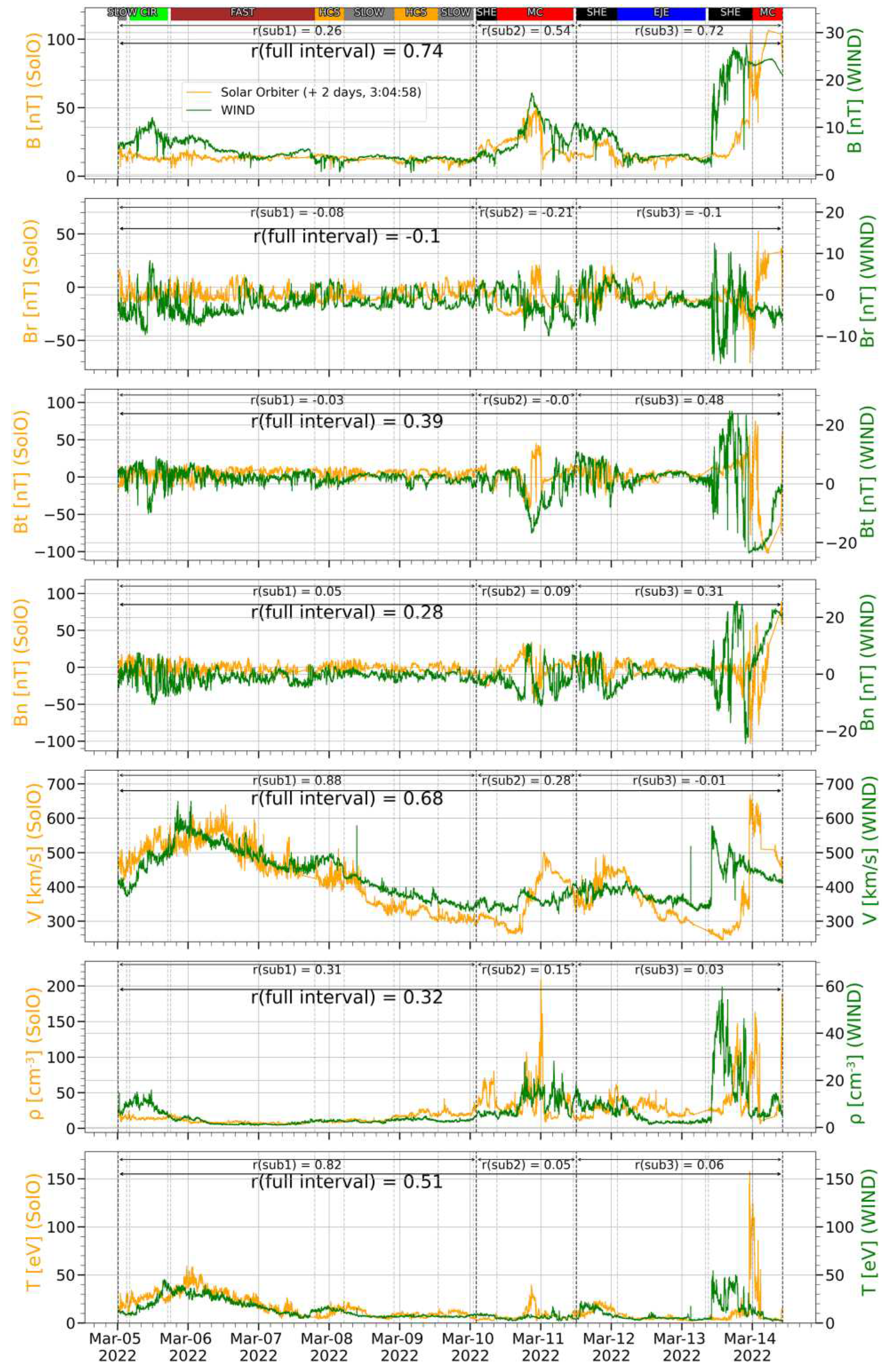
Comparison of simultaneous observations from two distant spacecraft (0.5 AU) provides a broader picture of the dynamics of the SW. Using the initial time-shift estimate (2 days, 3 hours and 5 minutes) by Formula 2, one of the highest levels of correlation with the mean value of 0.68 was observed for the bulk speed value, as in the first case (see Figure 8e). The second interval was also divided into three subintervals in accordance with the prominent plasma structures: sharp growth and smooth decline of the bulk speed in the first, oscillations in the second and surge after a stable section in the third. On the first subinterval (2022-03-02 21:05:00 UT — 2022-03-07 22:59:51 UT) the correlation coefficient of bulk speed is equal to 0.88, while on the second (2022-03-07 22:59:51 — 2022-03-09 08:59:51 UT) and third (2022-03-09 08:59:51 UT — 2022-03-12 07:11:00 UT) it drops sharply to 0.28 and -0.01 respectively (here latency corrections might be quite meaningful). At the same time, the average bulk speed value remained almost unchanged. Similar trends can be seen in the behavior of the correlation coefficient of the temperature time series (see Figure 5g), but its absolute value decreases several times over the propagation time. The IMF magnitude also significantly decreases with increasing distance (which is quite natural), but its correlation remains relatively high. The intervals containing SHEATH, EJECTA and MC have higher IMF magnitude correlation than for FAST and HCS. The time course in SLOW streams match well but correlation is worse, while the worst match is observed in CIR stream. The correlation level for the radial component of the IMF takes lower values (see Figure 8b), although for 0.1 AU, on the contrary, a higher correspondence of time series for this parameter was observed. The measurements of proton density illustrated in Figure 8f demonstrate the worst compliances among all the parameters under study. In the case of 0.1 AU, that parameter also has low compliance. Time series can undergo significant distortions at analyzed distances, but some prominent structures might persist for quite a long time. For example, Figure 8e shows that a rapid increase in bulk speed from ~300 to 650 km/s for the SolO and up to 550 km/s for WIND is observed on both spacecraft, although arrival times and the individual details of the time course after the interplanetary shock are different. Application of the corrected estimate (see section 2.4) for the third subinterval contributed to a significant increase in the level of correlation for almost all parameters (see Table 1).
3.2. Histogram analysis
First, we studied the distributions over the whole intervals. It was shown in the Section 3.1 that IMF magnitude and proton density demonstrate high variability when comparing data from two spacecraft even at relatively small distances (~0.1 AU). The full set of distributions for all considered parameters are presented on Figure 9. All distributions have a fairly broad shape. A statistical comparison showed that the distributions of IMF magnitude (Figure 9a), bulk speed (Figure 9c) and proton temperature (Figure 9d) change little as the SW flux advances at the analyzed distances (no more than 12% for magnetic field and temperature and no more than 3% for the bulk speed). Whereas noticeable discrepancy in the shape and basic characteristics of proton density (Figure 9b) distributions (median values differ by ~30%) is observed. At the same time the STD, standard errors of the mean and the normalized STD, reflecting the level of fluctuations at the interval, vary weakly for all quantities. All the above statistical characteristics are presented on Table 2.
Figure 8.
Time rows comparison of IMF magnitude (a) and its components in RTN system (b,c,d), bulk speed (e), proton density (f) and temperature observations (g) for the SolO and WIND (2nd event). All signatures are the same as in Figure 2.
Figure 8.
Time rows comparison of IMF magnitude (a) and its components in RTN system (b,c,d), bulk speed (e), proton density (f) and temperature observations (g) for the SolO and WIND (2nd event). All signatures are the same as in Figure 2.
The difference observed in distributions (especially for density, as the most variable parameter) may be because distributions are common to all observed large-scale structures, so the next step was to consider the distributions for type separately. We found remarkable features examining the histograms of parameter distributions for individual SW types. For example, the density distribution for the CIR (see Figure 10a) on the SolO has a complex shape with three peaks: the first subset of plasma with a density of ~7.5 cm-3, the second 9.5 cm-3 and the third 13.5 cm-3. However, when SW reaching WIND, two peaks with maximum at ~9 cm-3 and ~12.5 cm-3 can be observed instead of three peaks, observed on the SolO. Perhaps two strongly interacting streams merged into one during the propagation. Note that WIND was at this moment at a radial distance of about 0.1 AU from SolO, at the same time the distance between spacecrafts in the plane perpendicular Sun-Earth line was ~10⁶ km. Thus, the difference can be also related to inhomogeneities of plasma structures in space, as we can see different part of structures at different spacecraft.
However, it should be noted that no statistical characteristics of the distributions changed significantly as for density distributions over the entire 1st event as a whole.
The density distribution in the FAST stream also behaves differently at two spacecraft (see Figure 10b). It is noteworthy, that this type involves wide range of density values, including extremely high (not shown at histogram) compared to the average on the whole interval. So, to determine the mean and median values, the sample was limited to the range of the distribution in the figure. Two noticeably shifted maxima can be observed for density distributions on different spacecraft. The main distribution mode has a peak at 2.4 cm-3 for SolO which shifts to 1.3 cm-3 when approaching the WIND spacecraft.
Figure 10c present the density distributions for slow SW streams, which also have different shapes for SolO and WIND measurements, and differs from the distributions for CIR and FAST. These distributions also have a complex shape with several peaks, which suggests that not only large-scale structures can determine the shapes of distributions, but also their medium-scale substructures.
Thus, the statistical distributions for the density can change significantly even during the plasma motion time of ~9 hours at a distance of 0.1 AU and these changes might be different in various types of SW streams. That feature is specific to the proton density, such noticeable differences in statistical distributions are not observed for other observed parameters.
For the second event (0.5 AU between spacecraft), the histograms of the distributions are expectedly differ significantly depending on the parameter (see Figure 11 and Table 2). The distributions for the proton temperature were closest, even though its measurements on the SolO had a large scatter and reached 150 eV (the extreme values are rare and not shown in the Figure 11d). The bimodal bulk speed distribution (Figure 11c) registered at the SolO became more uniform when the flow reached WIND. These differences may also be due to the specifics of the measurements. The values of all statistical parameters remain approximately at the same level for the bulk speed and proton temperature by observation on both spacecraft (see Table 2). The histograms for the IMF magnitude (Figure 11a) have a clear similarity in the shape, but with significant shifted absolute values of the distribution maximum (mean and median values respectively), which is natural. However, normalized STD of IMF magnitude differs only by 20%. Density distributions (Figure 11b) have still the greatest differences in both shape and all statistical parameters (see Table 2, column 4 and 5). Despite the differences in distributions, normalized STD differs by only 25% on average but unlike other parameters for which the normalized STD decreases at 10-20% as the SW approaches the Earth, the STD for density, on the contrary, increases, i.e. the relative level of density fluctuations become greater.
In the case of proton density and the IMF magnitude, it is natural to observe significant differences in mean values, but the values of normalized STD, characterizing the relative level of fluctuations, change weakly for almost all observed parameters. Note that based on the value of the normalized STD, the level of fluctuations decreases slightly for all parameters except proton density, when SW moves to the Earth orbit. Whereas the relative density fluctuation on the contrary increase. Changes in the amplitudes of the analyzed parameters for spacecraft spacing 0.5 AU agree with the data in the existing models of SW propagation.
Consider the differences in statistical distributions on individual types of SW, as it was produced for previous interval, a number of peculiarities can be highlighted for the 2th event. For example, the IMF magnitude distribution in CIR streams (see Figure 12a) on SolO has a large peak and slight elevation, while on WIND, two peaks close in their values. However, the mean and median values differ less than for the same distributions of SW as a whole (Figure 11a). At the same time the other statistical parameters (the basic and normalized STD) are close for these two distributions and rather small values.
As the SW moves away from the Sun, it experiences various interactions with the surrounding space, which might affect its characteristics. It can be more pronounced for some types of SW. For example, distributions of IMF magnitude in HCS (see Figure 12b) have undergone significant changes both in form and in typical values. However normalized STD and STD parameters still remain at approximately the same level.
The distributions in slow SW (see Figure 12c) show again complicated picture with two distribution peaks (reflecting two plasma subsets). Wherein the relative positions of the peaks among themselves are preserved, but the role of each peak change - for SolO the main peak is posed at 13 nT, and the less pronounced peak is posed at 10nT, and for WIND oppositely the main peak have lower value ~3.5 nT, and the less significant peak has higher value~ 6.5 nT.
The analysis of the histograms for all types of SW showed that the greatest changes occur in SLOW, HCS and ICME (MC) streams. However, these conclusions are only preliminary, since a relatively small amount of statistical data has been collected so far for different SW types.
3.3. Fluctuation analysis
Analysis of the fluctuation level and its dynamics is an important step in the study of the evolution of SW structures. It was shown above that a noticeable change in the absolute value of the proton density might occur even at a small distance between spacecraft (0.1 AU). Nevertheless, the level of fluctuations (RSD values) and their time course are preserved at both selected events, and the observed changes are usually related to the type of the SW stream, as it was shown above. For example, Figure 13 shows the time course of the local normalized standard deviation (see the section Materials and Methods) of proton density for the first interval. One can see that in general the level of fluctuations is rather close on both spacecraft (with a difference of ~25% in average, while the fluctuation range in the observed fluctuations at each spacecraft is >500%). At the same time, some large-scale structures (FAST, HCS and CIR) a simultaneous increase in the level of fluctuations and the amplitudes of these increases are also close (with a difference of ~25%). However, for the FAST stream on November 7, in contrast, a noticeable difference is observed - the large peak of local normalized standard deviation for density can be seen on WIND data at 07/11/2021 ~ 04:00, however, it is not so by SolO data. This is due to the density structure, which is observed on WIND measurements and do not observe at SolO one (see Figure 5).
At a distance of 0.5 AU, there is a generally similar situation. It was shown earlier that significant changes in the absolute values of the parameters are possible, especially for IMF and proton density with increasing distance. Nevertheless, a weak change of local levels of fluctuations was observed for all of the studied SW parameters. In particular, the time course of the normalized standard deviation has similar and almost a point match at some places behavior for both spacecraft close (with a difference of 8% in average. It is significantly less than the fluctuation range on a single spacecraft equal more than >1000%), even for density of protons, which was the most variable parameter (see Figure 14). The time moments when a difference in the level of normalized standard deviation is visible is usually associated with some local structures observed on one spacecraft and not observed on another or observed with changing. For example, in the vicinity of magnetic cloud and interplanetary shocks occurred the greatest normalized standard deviation differences reaching values of 450%, which is still less than the fluctuation range on single spacecraft.
We have given a detailed comparison for density as the parameter with maximum level of fluctuations. For other parameters the situation for fluctuations is similar.
This result is consistent with the behavior of the fluctuations in case of the first event. In both cases, certain types of SW significantly increased the overall difference in mean values. For that reason, we can conclude that the level of local fluctuations almost does not change when the wind moves from the Sun to the Earth. However, it can vary for different types of SW (according to observations simultaneously on two spacecraft), an also for some local structures (observed on one of the spacecraft). Such local structures can be observed even in case of small distance between spacecraft, so it’s the result of spatial inhomogeneity of the SW, rather than evolution during movement.
3.4. Analysis of the 4th order moment of the PDF
In addition to the quite high coincidence of the amplitude and time course of the fluctuations of the SW parameters on different spacecraft, we can note that the distribution functions of the fluctuations of each of the parameters also have a similar form based on observations on both spacecraft. In this study, we analyzed the fluctuations of IMF magnitude, proton density and bulk speed. Figure 15 presents that the dependences of the flatness on the time scale at 0.1 AU has a similar character on the SolO and WIND. Overall, there is a decline of the flatness with scale, and at scales greater than 104 the flatness approaches three, which indicates the presence of intermittency in the discussed flows (see Section 2.7). Moreover, the level of intermittency for all quantities remains practically unchanged for each of the three subintervals. Nevertheless, we can note some differences in the behavior of the above-described dependences for different parameters. For example, the PDF for IMF fluctuations tends to the Gaussian distribution more smoothly than for the other parameters (see, for example, Figure 15a for the second subinterval of the first interval). However, for the density there are some differences at all scales, which is natural for such a variable parameter, wherein the trend in the 4th moment change is the same.
Flatness for the proton speed and density fluctuations persist at heliocentric distances from 0.9 AU to the libration point L1 along the Sun-Earth line. Meanwhile the variations for the IMF over scales are more uniformly distributed.
It can be noted that the character of shapes and features of the fluctuation distribution functions in the second event at a significant separation of spacecraft (~0.5 AU), in general, similar to previous event. Including the distribution function of the IMF and bulk speed fluctuations also smoothly approaches the normal distribution for both spacecraft (see for example Figure 16 for the second subinterval of the second event). For IMF magnitude (Figure 16a) there is an almost complete flatness match, while for bulk speed (Figure 16b) there are discrepancies by the level of flatness. The largest discrepancy of flatness is still observed for the proton density (Figure 16c). The distribution tails become lighter and large amplitude fluctuations become less frequent for the WIND plasma measurements. That fact might indicate a decrease in the level of intermittency during plasma propagation to the Earth. However, such tendency is observed for many but not for all intervals. The flatness, calculated on several subintervals, show a large scatter and require more in-depth analysis.
In general, a similar pattern is observed for the most intervals. As a result, we can conclude that the characteristics of intermittency, one of the characteristics of the turbulent SW flow in general vary weakly with distance for most parameters. Nevertheless, for in some parameters in some subintervals these differences can be significant, which requires more depth research.
4. Discussion
In this study we investigated two long intervals of simultaneous observations on the SolO and WIND spacecraft located at a distance of 0.1 and 0.5 AU from each other. The dynamics of SW structures was analyzed in a wide range of scales due to the use of long data series with high temporal resolution. The high correspondence of observations on the two spacecraft for most analysis at the close location of spacecraft indicates the correctness of the accuracy of methods of data selection and correction (see section 2.4) and the possibility to compare observations even at significant distances of spacecraft.
We used correlation analysis method described by [36] to find the optimal time shift and compare the SW parameters, which allowed us to increase the level of correlation of large-scale structures and trace its evolution. In addition, we were able to examine the effect of different types of SW on the level of correlation and identify the most variable and stable physical quantities and SW stream phenomena. The bulk speed was the most unchanging parameter, while the proton density and magnetic field parameters varied the most.
In [19] the use of multipoint measurements from five spacecraft helped to broadly describe 17 CME phenomena, finding their complex structure with several components and exhibit different behavior depending on the distance to the Sun. Our research was aimed at studying a similar set of SW and IMF parameters used data from only two spacecraft with measurements taken near the Sun-Earth line but at different distance from the Sun, which allowed us to detect and study evolution of fluctuations and its differences in a few CIRs and ICME (MC) streams phenomena near the Sun-Earth line that may be geoeffective.
Our study included not only comparison of time series, but also statistical analysis. In particular, we analyzed histograms of SW parameters in general and in different stream types with wide range of statistical parameters. Note that if the changing in absolute value of proton density and magnetic field magnitude looks quite natural, it is rather surprising that the normalized STD, which roughly reflect the level of fluctuations in the flow varies slightly with SW propagating for almost all discussed parameters.
The more complicated parameter distributions and largest changes are observed for SLOW, HCS and ICME(MC) SW types. The complicated distribution form can be related with complex set of substructures inside the above large-scale structures. On the other hand, similar distributions are often observed in the SW, and may be the result of the addition of different plasma populations [37]. In this study, we have demonstrated only a small fraction of the collected statistics for different types of SW, focusing on only two physical quantities. More detailed studies are planned that will expand our understanding of the statistical properties of the various streams and its dynamics.
An important stage of this work was the consideration of fluctuations properties in SW streams. The research of local normalized standard deviations at three-hour subintervals using multipoint comparisons of the analyzed parameters made it possible to understand on dynamics of fluctuation levels and influence of different SW types on this process. The average local fluctuation level varies little regardless of distance, but it can vary significantly with SW type. At the same time the great difference of the local fluctuation level at two points can indicate some plasma structures observed only at one spacecraft. Moreover, such situations can be observed even at small distance between observation point along Sun-Earth line. It can't be explained by SW evolution during propagation, and are most likely the result of SW flow inhomogeneity in the direction perpendicular to Sun-Eath line that is, the limited size of the structure in this plane.
In the last stage fluctuation analysis, we investigated SW inhomogeneity with use of PDF of fluctuations research at different time scales consideration. We used an approach similar to [21,39]) and other analogous papers. Bruno & Carbone [21] have found a difference in dynamics in the intermittency of bulk speed and IMF components between FAST and SLOW streams within long observation intervals, where only FAST wind intermittency increases with radial distance. The growing of intermittency with distance from the Sun was also shown in [22] by measurements from Ulysses and ACE. At the current stage of the study, we have considered the behavior of flatness for the stream as a whole and found no significant differences in the intermittency properties of the SolO and WIND data, regardless of the distance between them, including proton density (more variable parameter). In some cases, there is even an increase in intermittency when approaching the Earth. However, more detailed analysis is required to draw accurate conclusions regarding the evolution of intermittency over long distances.
5. Conclusions
The main results of this research are:
On average, a high level of correlation between the time series of SW and IMF parameters is observed both at a distance of 0.1 and at 0.5 AU (the average the correlation coefficient is more than 0.5);
The bulk speed is subject to the smallest changes (mean correlation coefficient about 0.8), the IMF magnitude and proton density are the most variable parameters;
The level of correlation may significantly vary for different large-scale types of SW;
Mainly the levels of relative fluctuations persist at distances of 0.1 and 0.5 AU for all parameters, regardless of changes in their amplitudes;
Local fluctuation levels also vary weakly with distance and might be change in general in different types of SW streams or on some plasma structures;
The degree of non-Gaussianity of the PDF is preserved, which may indicate that the level of intermittency is also unchanged with the movement of SW streams.
The conducted research presented analysis at different distances on the way from the Sun to the Earth has the potential to enhance predictions of space weather, specifically by developing more advanced techniques for tracking solar phenomena and their impact on the Earth.
Author Contributions
Conceptualization, M.R. and Y.Y.; methodology, I.V., M.R. and L.R.; software, I.V.; validation, M.R. and L.R.; investigation, I.V.; writing—original draft preparation, I.V. and M.R.; writing—review and editing, I.V. and M.R.; visualization, I.V. and A.K.; supervision, Y.Y. All authors have read and agreed to the published version of the manuscript.
Funding
This research was funded by the Russian Science Foundation, grant 22-12-00227.
Data Availability Statement
All data utilized is openly accessible. Coordinated Data Analysis Web (URL: https://cdaweb.gsfc.nasa.gov/), Catalog of large-scale solar wind structures (URL: http://iki.rssi.ru/pub/omni/catalog/)
Acknowledgments
We would like to express my sincere gratitude to the creators of the CDAweb database and OMNI catalog as well as the leaders of the experiments whose data we have used.
Conflicts of Interest
The authors declare no conflict of interest.
References
- Marsch, E. Solar Wind Models from the Sun to 1 AU: Constraints by in Situ and Remote Sensing Measurements. Space Sci. Rev. 1999, 87, 1–24. [Google Scholar] [CrossRef]
- Verscharen, D.; Klein, K.G.; Maruca, B.A. The multi-scale nature of the solar wind. Living Rev. Sol. Phys. 2019, 16, 5. [Google Scholar] [CrossRef] [PubMed]
- Petrukovich, A.A.; Malova, H.V.; Popov, V.Y.; Maiewski, E.V.; Izmodenov, V.V.; Katushkina, O.A.; Vinogradov, A.A.; Riazantseva, M.; Rakhmanova, L.S.; Podladchikova, T.V.; et al. Modern view of the solar wind from micro to macro scales. Physics-Uspekhi 2020, 63, 801–811. [Google Scholar] [CrossRef]
- Feldman, W.C.; Asbrige, J.R.; Bame, S.J.; Gosling, J.T. Longterm variations of selected solar wind properties: IMP 6, 7 and 8 results. J. Geophys. Res. Space Phys. 1978, 83, 2177–2189. [Google Scholar] [CrossRef]
- Schwenn, R. Solar Wind Sources and Their Variations over the Solar Cycle. In Solar Dynamics and Its Effects on the Heliosphere and Earth; Baker, D.N., Klecker, B., Schwartz, S.J., Schwenn, R., Von Steiger, R., Eds.; Space Sciences Series of ISSI; Springer: New York, NY, USA, 2007; Volume 22, pp. 51–76. [Google Scholar] [CrossRef]
- Yermolaev, Yu.I.; Nikolaeva, N.S.; Lodkina, I.G.; Yermolaev, M.Yu. Catalog of Large-Scale Solar Wind Phenomena during 1976–2000. Cosm. Res. 2009, 47, 81–94. [Google Scholar] [CrossRef]
- Kilpua, E.K.J.; Balogh, A.; Von Steiger, R.; Liu, Y.D. Geoeffective Properties of Solar Transients and Stream Interaction Regions. Space Sci. Rev. 2017, 212, 1271–1314. [Google Scholar] [CrossRef]
- Marsch, E. MHD Turbulence in the Solar Wind. In Physics of the Inner Heliosphere II. Particles, Waves and Turbulence; Schwenn, R., Marsch, E., Eds.; Physics and Chemistry in Space; Springer: Berlin, Heidelberg, Germany, 1991; Volume 21, pp. 159–241. [Google Scholar] [CrossRef]
- Bavassano, B. The solar wind: A turbulent magnetohydrodynamic medium. Space Sci. Rev. 1996, 78, 29–32. [Google Scholar] [CrossRef]
- Tsurutani, B.T.; Ho, C.M. A review of discontinuities and Alfvén waves in interplanetary space: Ulysses results. Rev. Geophys. 1999, 37, 517–541. [Google Scholar] [CrossRef]
- Borovsky, J.E. On the flux-tube texture of the solar wind: Strands of the magnetic carpet at 1 AU? J.Geophys. Res. Space Phys. 2008, 113, A08110. [Google Scholar] [CrossRef]
- Hudson, P.D. Discontinuities in an anisotropic plasma and their identification in the solar wind. Planetary and Space Science 1970, 18, 1611–1622. [Google Scholar] [CrossRef]
- Taylor, G.I. The Spectrum of Turbulence. Proc. R. Soc. Lond. Ser. - Math. Phys. Sci. 1997, 164, 476–490. [Google Scholar] [CrossRef]
- Burlaga, L.; Sittler, E.; Mariani, F.; Schwenn, R. Magnetic loop behind an interplanetary shock: Voyager, Helios, and IMP 8 observations. J. Geophys. Res. 1981, 86, 6673–6684. [Google Scholar] [CrossRef]
- Prise, A.J.; Harra, L.K.; Matthews, S.A.; Arridge, C.S.; Achilleos, N. Analysis of a coronal mass ejection and corotating interaction region as they travel from the Sun passing Venus, Earth, Mars, and Saturn. J. Geophys. Res. Space Phys. 2015, 120, 1566–1588. [Google Scholar] [CrossRef]
- Lugaz, N.; Winslow, R.M.; Farrugia, C.J. Evolution of a long-duration coronal mass ejection and its sheath region between Mercury and Earth on 9–14 July 2013. J. Geophys. Res. Space Phys. 2020, 125, e2019JA027213. [Google Scholar] [CrossRef]
- Good, S.W.; Kilpua, E.K. J.; LaMoury, A.T.; Forsyth, R.J.; Eastwood, J.P.; Möstl, C. Self-similarity of ICME flux ropes: Observations by radially aligned spacecraft in the inner heliosphere. J. Geophys. Res. Space Phys. 2019, 124, 4960–4982. [Google Scholar] [CrossRef]
- Möstl, C.; Farrugia, C.J.; Kilpua, E.K. J.; Jian, L.K.; Liu, Y.; Eastwood, J.P.; Harrison, R.A.; Webb, D.F.; Temmer, M.; Odstrcil, D.; et al. Multipoint shock and flux rope analysis of multiple interplanetary coronal mass ejections around 2010 August 1 in the inner heliosphere. Astrophys. J. 2012, 758, 18. [Google Scholar] [CrossRef]
- Möstl, C.; Weiss, A.J.; Reiss, M.A.; Amerstorfer, T.; Bailey, R.L.; Hinterreiter, J.; Bauer, M.; Barnes, D.; Davies, J.A.; Harrison, R.A.; et al. Multipoint Interplanetary Coronal Mass Ejections Observed with Solar Orbiter, BepiColombo, Parker Solar Probe, Wind, and STEREO-A. Astrophys. J. Lett. 2022, 924, L. [Google Scholar] [CrossRef]
- Bruno, R.; Carbone, V. The Solar Wind as a Turbulence Laboratory. Living Rev. Sol. Phys. 2013, 10, 2. [Google Scholar] [CrossRef]
- Bruno, R.; Carbone, V.; Sorriso-Valvo, L.; Bavassano, B. Radial evolution of solar wind intermittency in the inner heliosphere. J. Geophys. Res. 2003, 108, 1130. [Google Scholar] [CrossRef]
- D’Amicis, R.; Bruno, R.; Pallocchia, G.; Bavassano, B.; Telloni, D.; Carbone, V.; Balogh, A. Radial Evolution of Solar Wind Turbulence during Earth and Ulysses Alignment of 2007 August. Astrophys. J. 2010, 717, 474–480. [Google Scholar] [CrossRef]
- Bruno, R.; Trenchi, L. Radial Dependence of the Frequency Break between Fluid and Kinetic Scales in the Solar Wind Fluctuations. Astrophys. J. Lett. 2014, 787, L24. [Google Scholar] [CrossRef]
- Telloni, D. Spacecraft radial alignments for investigations of the evolution of solar wind turbulence: A review. J. Atmosph. Sol.–Ter. Phys. 2023, 242, 105999. [Google Scholar] [CrossRef]
- Alberti, T.; Milillo, A.; Heyner Hadid, L.Z.; Auster, H.-H.; Richter, I.; Narita, Ya. The “Singular” Behavior of the Solar Wind Scaling Features during Parker Solar Probe– BepiColombo Radial Alignment. Astrophys. J., 2022, 926, 174. [Google Scholar] [CrossRef]
- Telloni, D.; Sorriso-Valvo, L.; Woodham, L.D.; Panasenco, O.; Velli, M.; Carbone, F.; Zank, G.P.; Bruno, R.; Perrone, D.; Nakanotani, M.; et al. Evolution of Solar Wind Turbulence from 0.1 to 1 au during the First Parker Solar Probe–Solar Orbiter Radial Alignment. Astrophys. J. Lett. 2021, 912, 8. [Google Scholar] [CrossRef]
- Sioulas, N.; Velli, M.; Huang, Z.; Shi, C.; Bowen, T.A.; Chandran B. D., G.; Liodis, I.; Davis, N.; Bale, S.D.; Horbury, T.S.; et al. On the Evolution of the Anisotropic Scaling of Magnetohydrodynamic Turbulence in the Inner Heliosphere. Astrophys. J 2023, 951, 12. [Google Scholar] [CrossRef]
- Lepping, R.P.; Acũna, M.H.; Burlaga, L.F.; Farrell, W.M.; Slavin, J.A.; Schatten, K.H.; Mariani, F.; Ness, N.F.; Neubauer, F.M.; Whang, Y.C.; et al. The Wind Magnetic Field Investigation. Space Sci. Rev. 1995, 71, 207–229. [Google Scholar] [CrossRef]
- Lin, R.P.; Anderson, K.A.; Ashford, S.; Carlson, C.; Curtis, D.; Ergun, R.; Larson, D.; McFadden, J.; McCarthy, M.; Parks, G.K.; et al. A Three-Dimensional Plasma and Energetic Particle Investigation for the Wind Spacecraft. Space Sci. Rev. 1995, 71, 125–153. [Google Scholar] [CrossRef]
- Ogilvie, K.W.; Chornay, D.J.; Fritzenreiter, R.J.; Hunsaker, F.; Keller, J.; Lobell, J.; Miller, G.; Scudder, J.D.; Sittler, E.C.; Torbert, R.B.; et al. SWE, a Comprehensive Plasma Instrument for the WIND Spacecraft. Space Sci. Rev. 1995, 71, 55–77. [Google Scholar] [CrossRef]
- Horbury, T.S.; O’Brien, H.; Carrasco Blazquez, I.; Bendyk, M.; Brown, P.; Hudson, R.; Evans, V.; Oddy, T.M.; Carr, C.M.; Beek, T.J.; et al. The Solar Orbiter Magnetometer. Astron. Astrophys. 2020, 642, A9. [Google Scholar] [CrossRef]
- Owen, C.J.; Bruno, R.; Livi, S.; Louarn, P.; Janabi, K.A.; Allegrini, F.; Amoros, C.; Baruah, R.; Barthe, A.; Berthomier, M.; et al. The Solar Orbiter Solar Wind Analyser (SWA) Suite. Astron. Astrophys. 2020, 642, A16. [Google Scholar] [CrossRef]
- Yermolaev, Y.I.; Lodkina, I.G.; Yermolaev, M.Y. Dynamics of large-scale solar-wind streams obtained by the double superposed epoch analysis: 3. Deflection of the velocity vector. Sol. Phys. 2018, 293, 91. [Google Scholar] [CrossRef]
- Thompson, W.T. Coordinate systems for solar image data. Astron. Astrophys. 2006, 449, 791–803. [Google Scholar] [CrossRef]
- Weimer, D.; King, J. Improved Calculations of Interplanetary Magnetic Field Phase Front Angles and Propagation Time Delays. J. Geophys. Res. 2008, 113. [Google Scholar] [CrossRef]
- Rakhmanova, L.S.; Riazantseva, M.O.; Zastenker, G.N. Solar-Wind Structure Propagation through the Magnetosheath Studied by Two Themis Probes. Cosm. Res. 2015, 53, 331–340. [Google Scholar] [CrossRef]
- Berčič, L.; Maksimović, M.; Landi, S.; Matteini, L. Scattering of Strahl Electrons in the Solar Wind between 0.3 and 1 Au: Helios Observations. Mon. Not. R. Astron. Soc 2019, 486, 3404–3414. [Google Scholar] [CrossRef]
- Riazantseva, M.O.; Budaev, V.P.; Rakhmanova, L.S.; Zastenker, G.N.; Šafránková, J.; Němeček, Z.; Přech, L. Comparison of Properties of Small-Scale Ion Flux Fluctuations in the Flank Magnetosheath and in the Solar Wind. Adv. Space Res. 2016, 58, 166–174. [Google Scholar] [CrossRef]
- Sorriso-Valvo, L.; Carbone, V.; Veltri, P.; Consolini, G.; Bruno, R. Intermittency in the Solar Wind Turbulence through Probability Distribution Functions of Fluctuations. Geophys. Res. Lett. 1999, 26, 1801–1804. [Google Scholar] [CrossRef]
Figure 1.
Trajectory and coordinates of SolO spacecraft (orange square) and WIND (green circle) in HEEQ coordinates: (a) The first selected event - 0.1 AU between spacecraft; (b) The second selected event - 0.5 AU between spacecraft.
Figure 1.
Trajectory and coordinates of SolO spacecraft (orange square) and WIND (green circle) in HEEQ coordinates: (a) The first selected event - 0.1 AU between spacecraft; (b) The second selected event - 0.5 AU between spacecraft.
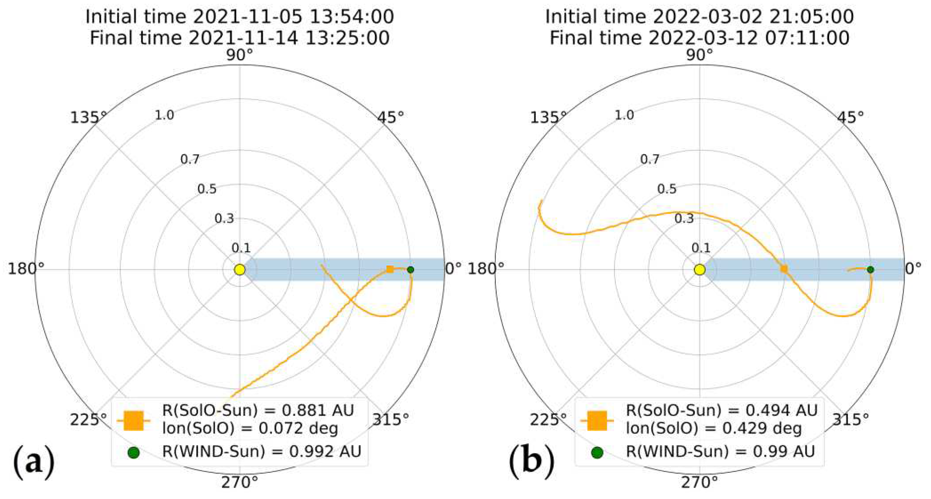
Figure 2.
(a) Comparison of proton bulk speed (top panel) and proton temperature (bottom panel) time rows observations for the SolO and WIND with preliminary time shift (2nd event). Correlation coefficients for full interval (r(full interval)) and for subintervals (r(sub...)) are shown at the chart. The color bar at the top of the chart shows the periods of different SW large scale structures according to section 2.1; (b) Dependence of the correlation coefficient between bulk speed values time rows measured at SolO and WIND on the time shift between them; (c) Comparison of proton temperature time rows observations at the SolO and WIND for the third subinterval with time shift estimate by correlation analysis (3rd subinterval of the 2nd event).
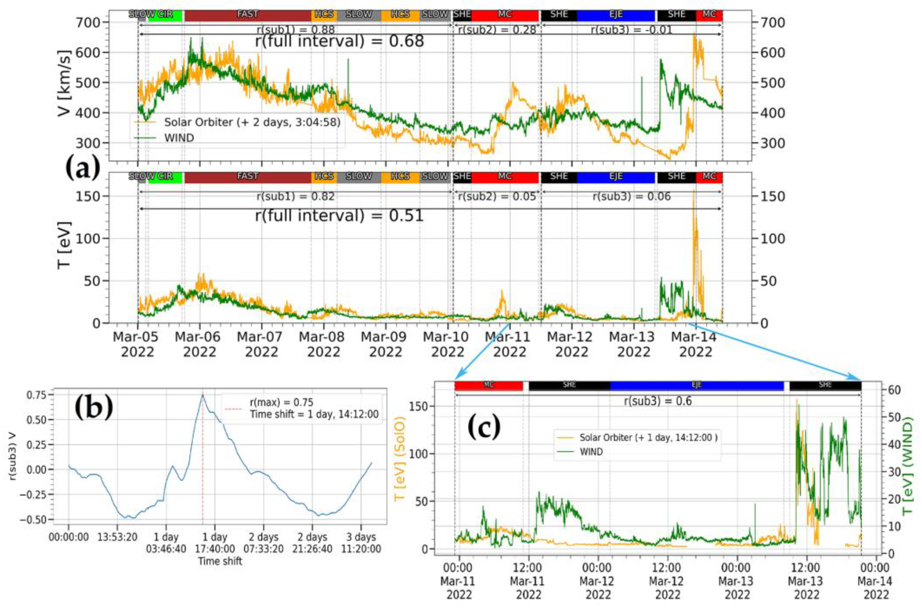
Figure 3.
The behavior of the local normalized standard deviation (the measure of fluctuations level) of the IMF magnitude for the SolO and WIND for the first subinterval of the 1st event (12:00 7th – 12:00 9th of November 2021).
Figure 3.
The behavior of the local normalized standard deviation (the measure of fluctuations level) of the IMF magnitude for the SolO and WIND for the first subinterval of the 1st event (12:00 7th – 12:00 9th of November 2021).
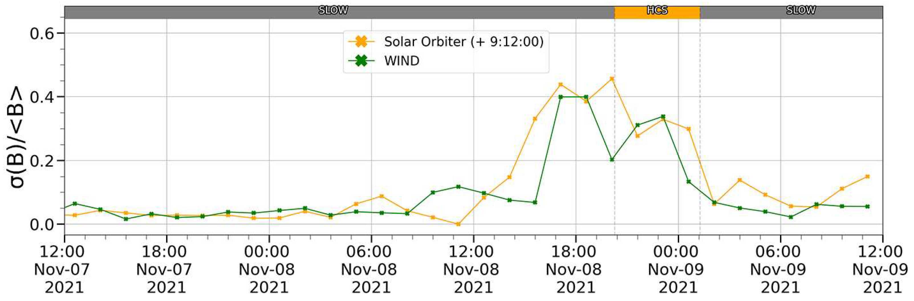
Figure 4.
(a) PDF for the fluctuations of the IMF magnitude on the SolO (orange line) and on the WIND (green line) and its comparison with the Gaussian distribution (black dashed line); (b) Flatness of the IMF magnitude fluctuations dependence on the time scale of fluctuations in the logarithmic scale for the SolO (orange line) WIND (green line) (1st event, 1st subinterval).
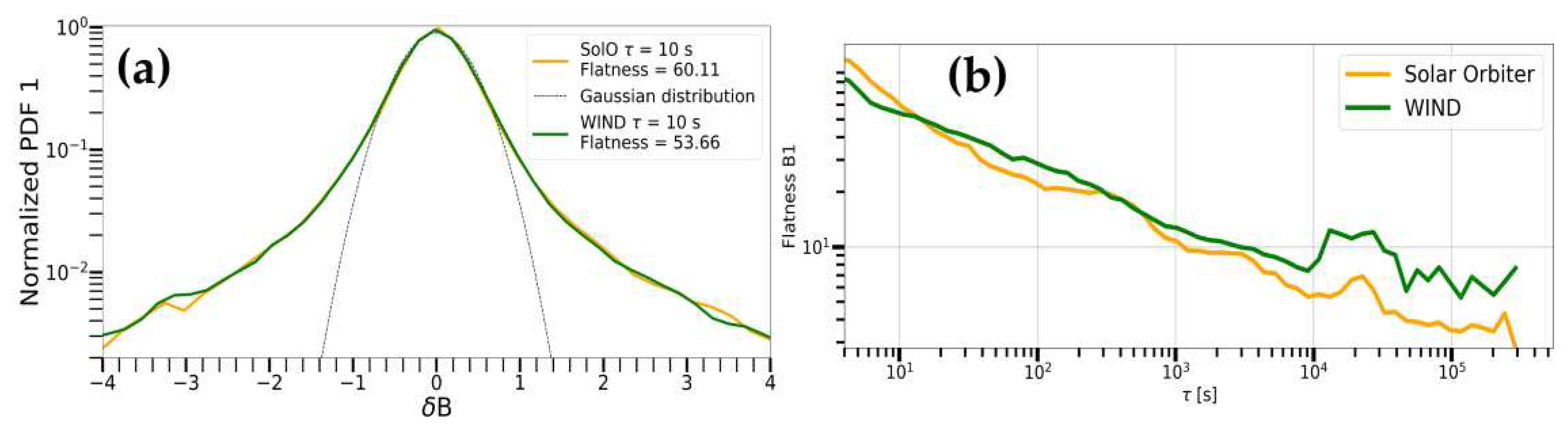
Figure 5.
Time rows comparison of the IMF magnitude (a) and its components in RTN system (b,c,d), bulk speed (e), proton density (f) and temperature (g) for the SolO and WIND observations (1st event). The values of correlation coefficients are signed on the graph the same as on Figure 2a. Сcorrelation coefficients after refining the time shift for each subinterval are presented in Table 1.
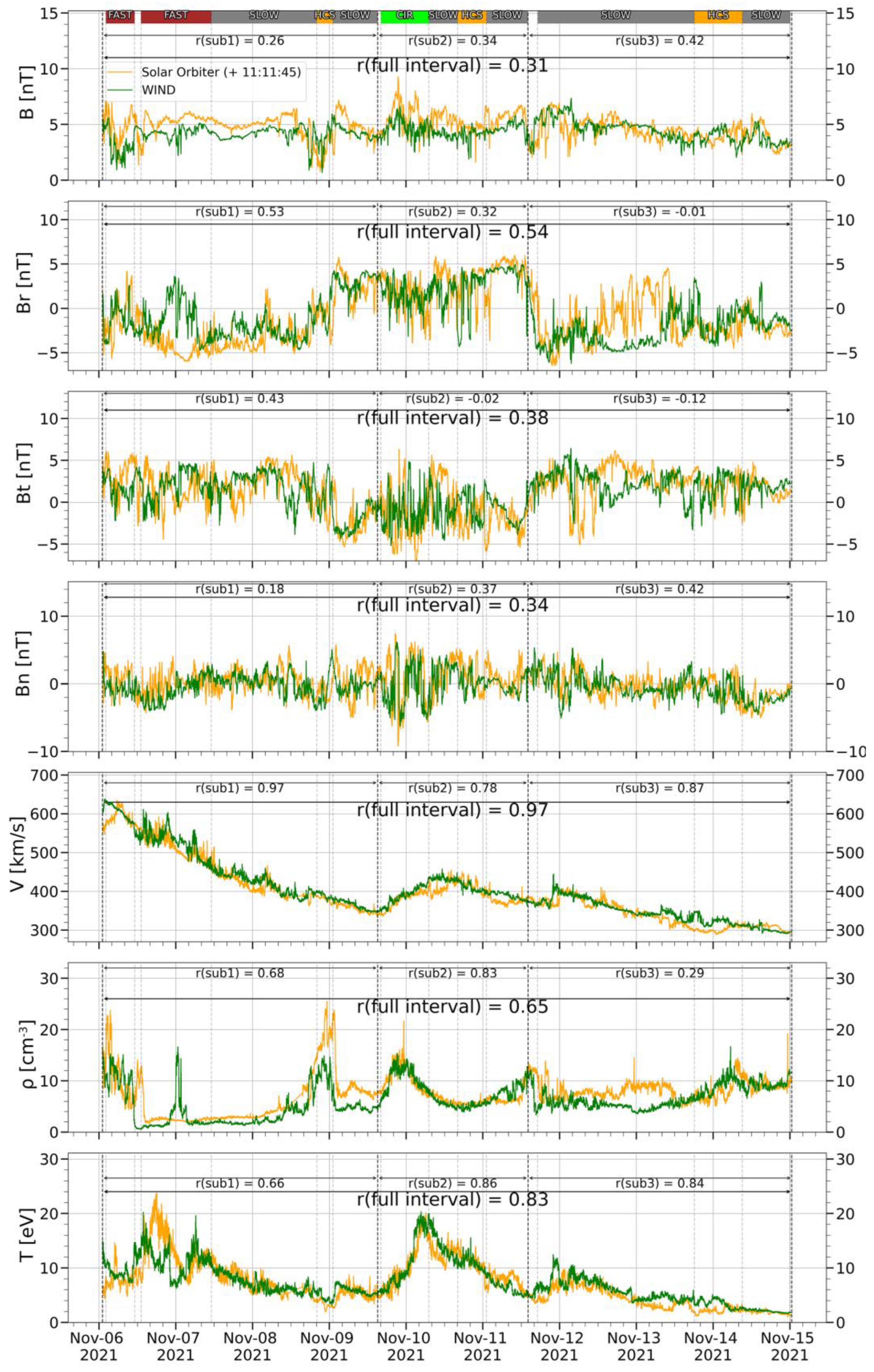
Figure 6.
Comparison of bulk speed time rows for the third subinterval (1st event) with taking into account the finalized time shift. The color bar at the top of the chart shows the periods of different SW large scale structures according to section 2.1. Correlation coefficients for full 3rd subinterval (r) and for different SW structures (r1,r2,r3) are shown at the chart.
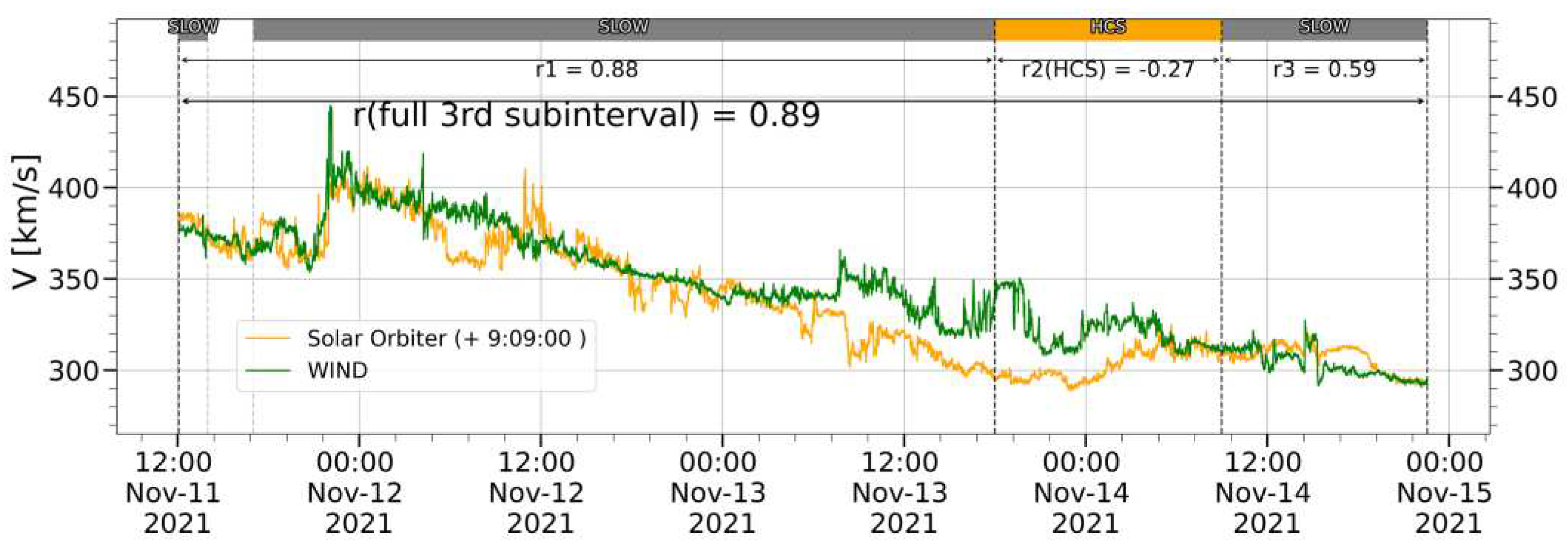
Figure 7.
Comparison of IMF components time rows for the first subinterval (1st event). (a) Radial; (b) Tangential; (c) Normal. Correlation coefficients after refinement of the time shift are indicated.
Figure 7.
Comparison of IMF components time rows for the first subinterval (1st event). (a) Radial; (b) Tangential; (c) Normal. Correlation coefficients after refinement of the time shift are indicated.
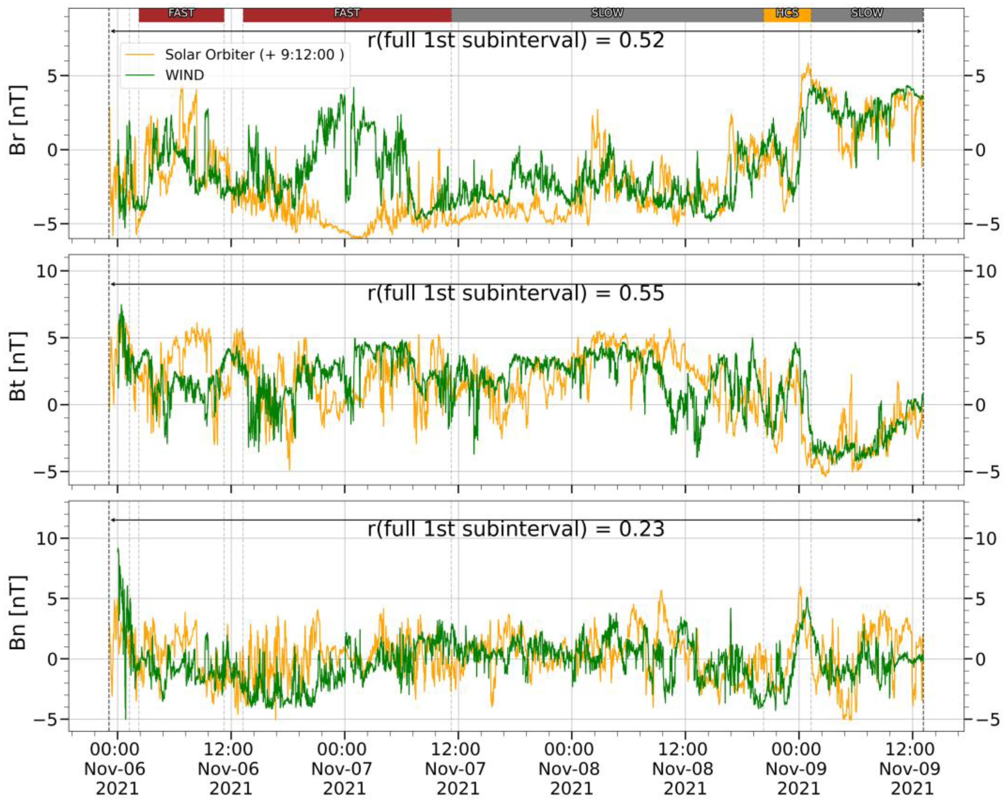
Figure 9.
Comparison of distribution histograms (1st event). (a) IMF magnitude; (b) SW proton density; (c) SW bulk speed; (d) SW proton temperature.
Figure 9.
Comparison of distribution histograms (1st event). (a) IMF magnitude; (b) SW proton density; (c) SW bulk speed; (d) SW proton temperature.
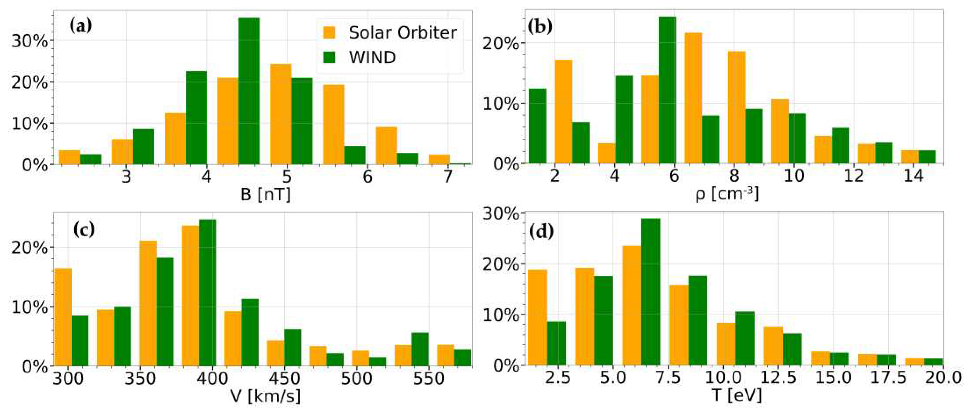
Figure 10.
Density distributions in CIR (a), FAST (b), and slow SW (c) (1st event).
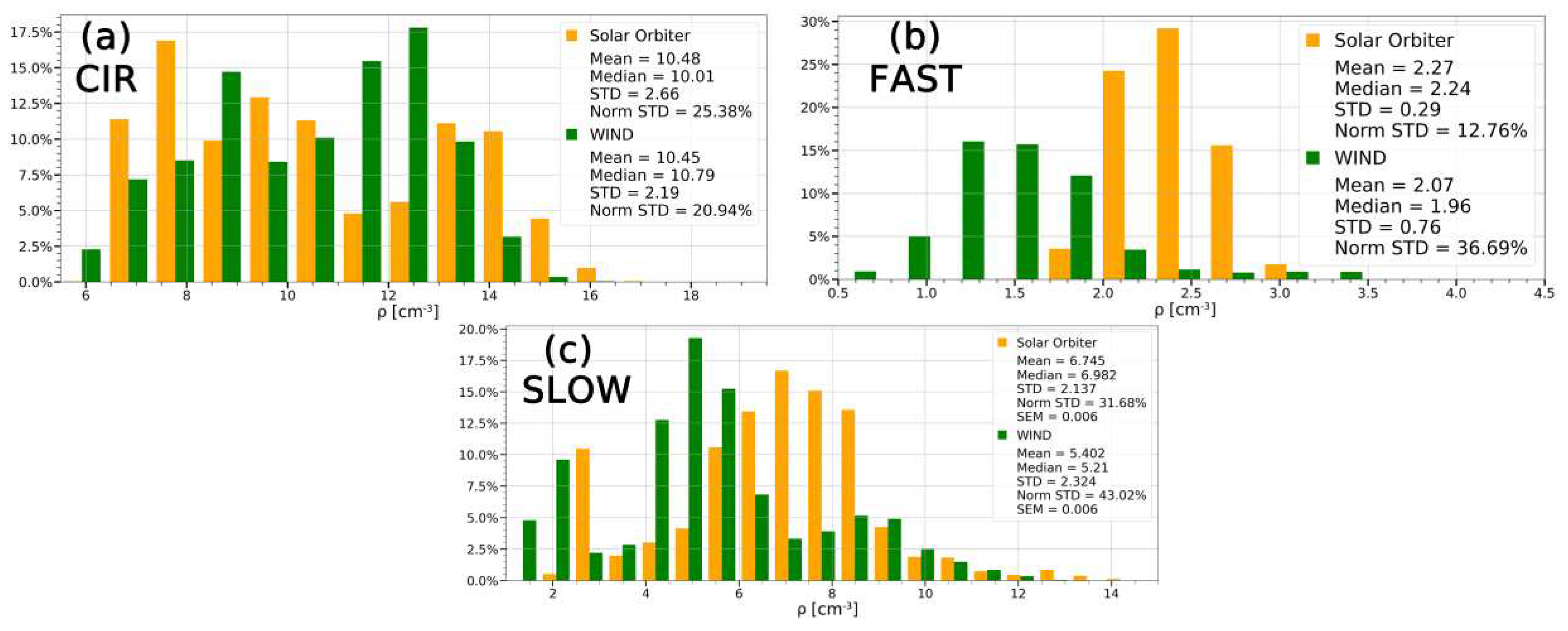
Figure 11.
Comparison of distribution histograms (2nd event). (a) IMF magnitude; (b) Proton density; (c) Bulk speed; (d) Proton temperature.
Figure 11.
Comparison of distribution histograms (2nd event). (a) IMF magnitude; (b) Proton density; (c) Bulk speed; (d) Proton temperature.
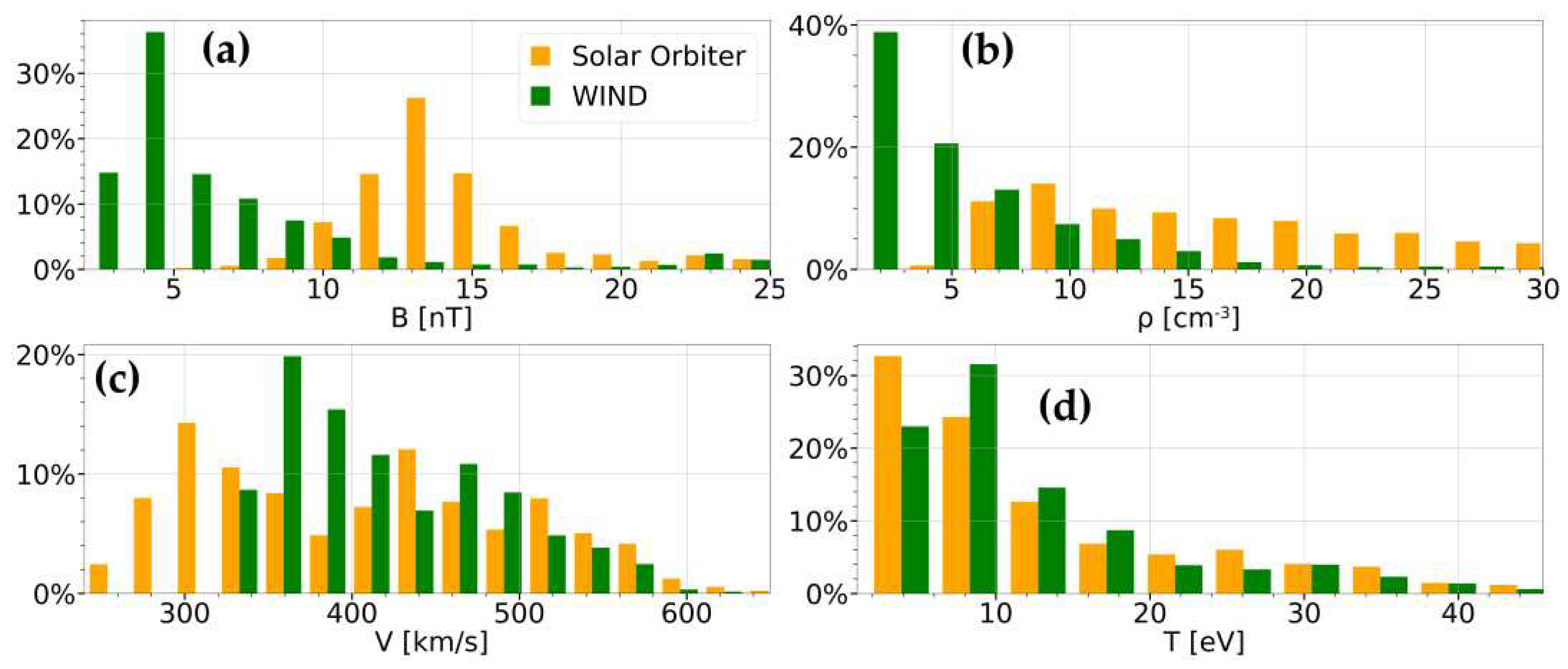
Figure 12.
IMF magnitude distributions in CIR (a), HCS (b), and slow SW (c) ((2nd event).
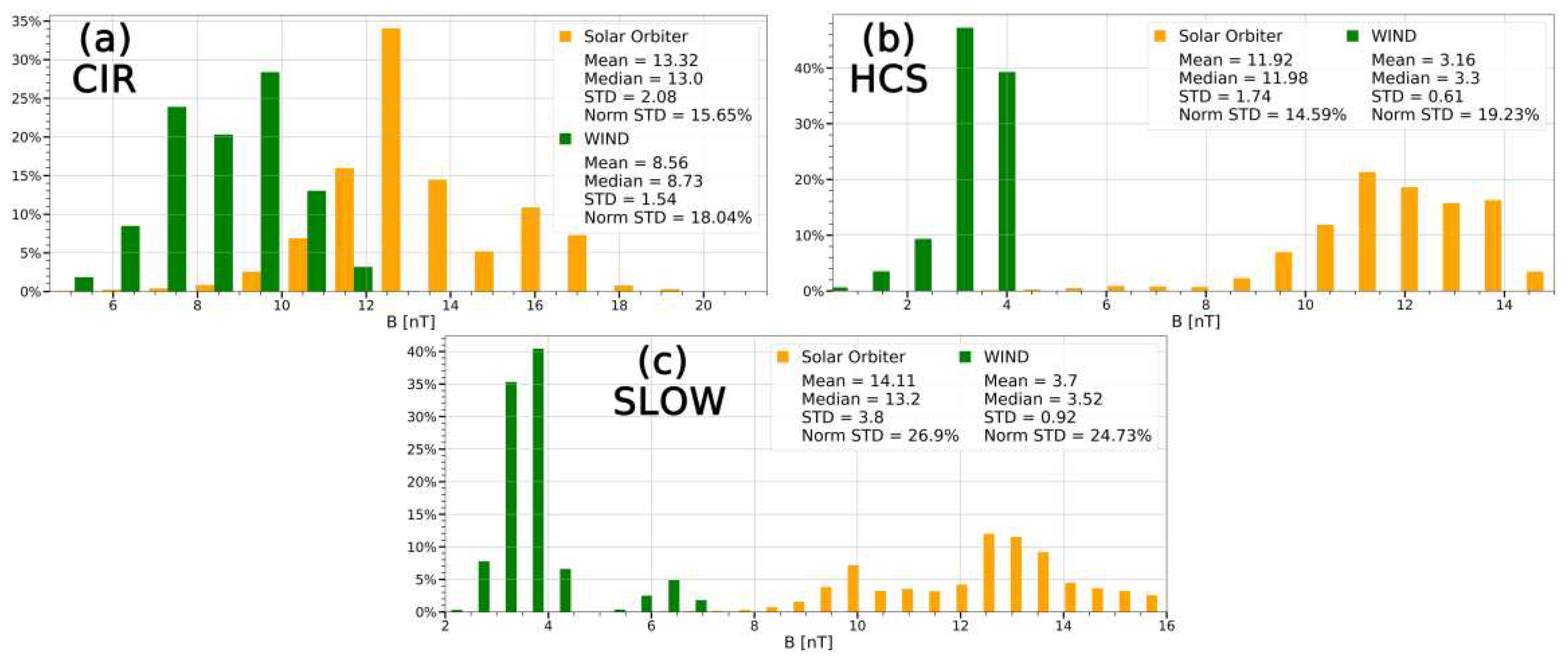
Figure 13.
Behavior of the fluctuation level for proton density (1st event).
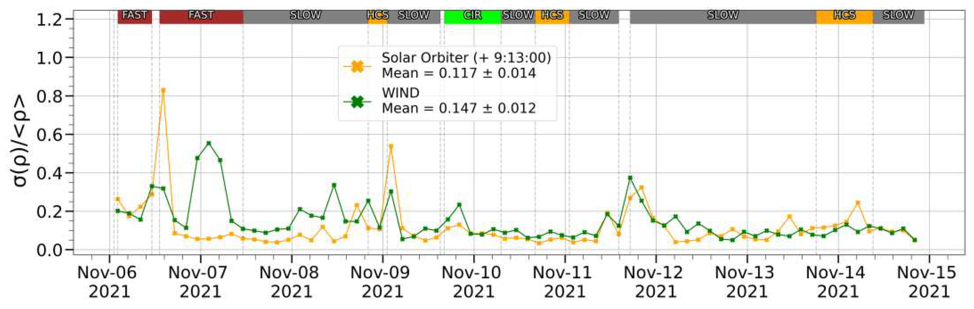
Figure 14.
Behavior of the fluctuation level for proton density (2nd event).
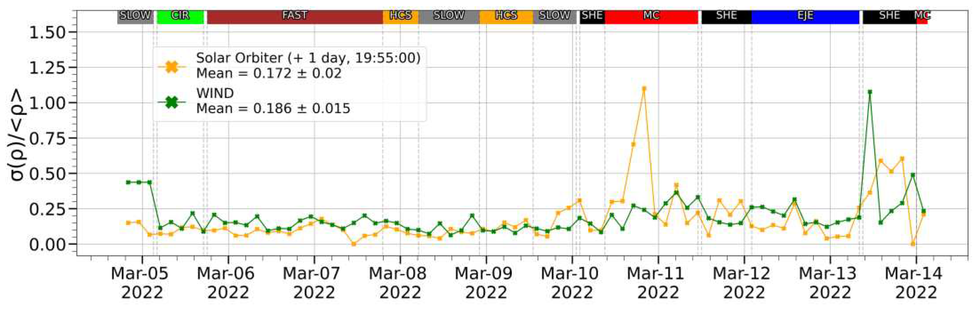
Figure 15.
Comparison of the dependence of Flatness at the second subinterval of the (1st event). (a) IMF magnitude; (b) Bulk speed; (c) Proton density.
Figure 15.
Comparison of the dependence of Flatness at the second subinterval of the (1st event). (a) IMF magnitude; (b) Bulk speed; (c) Proton density.
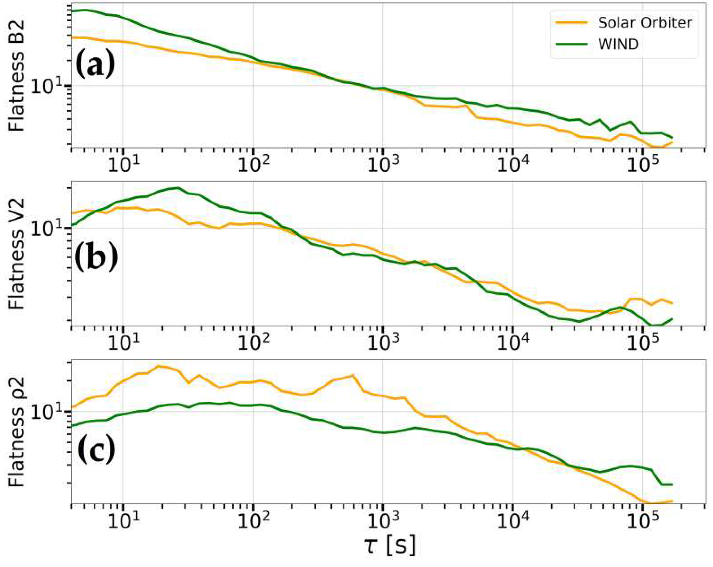
Figure 16.
Comparison of the dependence of Flatness at the second subinterval of the (2nd event). (a) IMF magnitude; (b) Bulk speed; (c) Proton density.
Figure 16.
Comparison of the dependence of Flatness at the second subinterval of the (2nd event). (a) IMF magnitude; (b) Bulk speed; (c) Proton density.
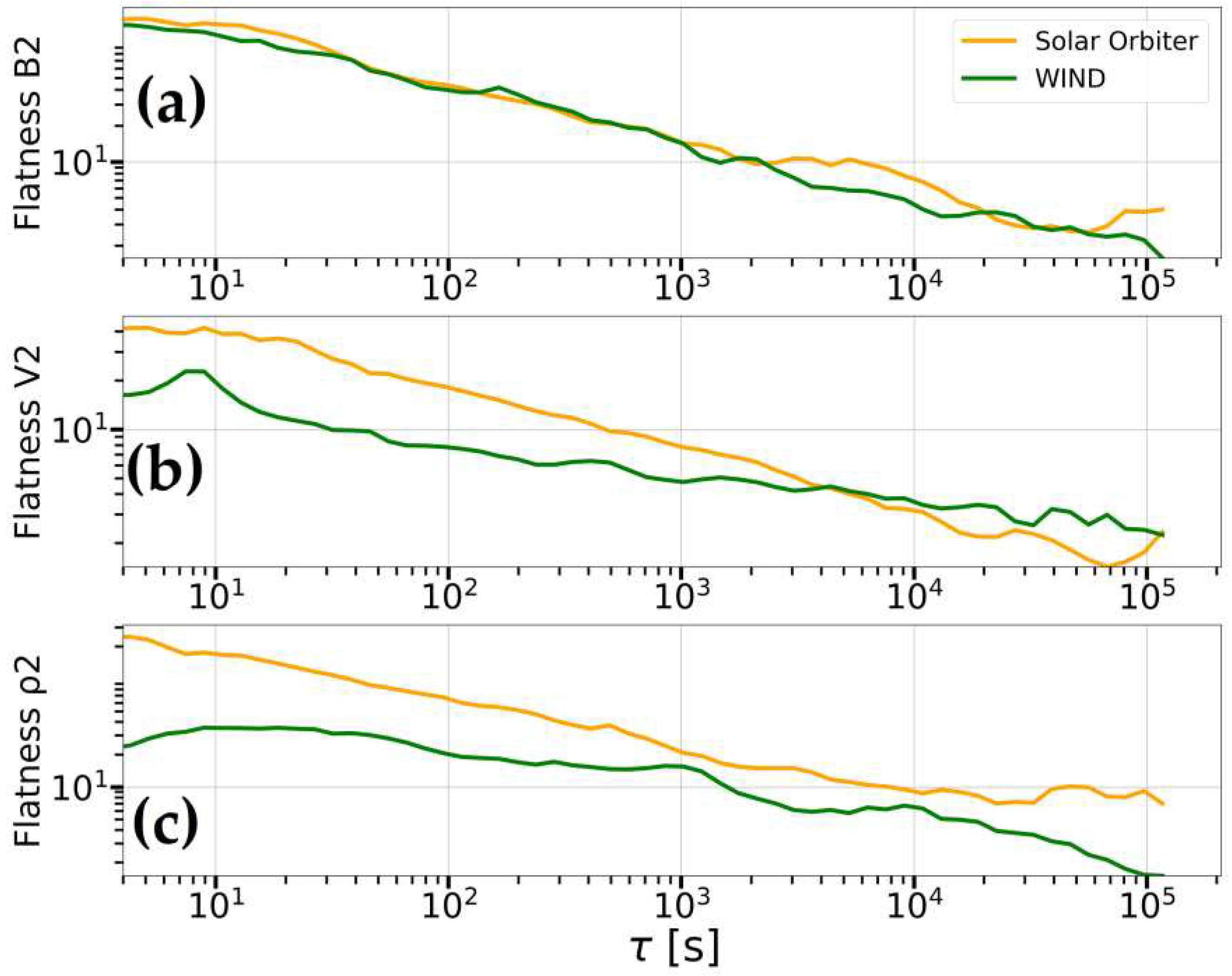

Table 1.
Comparison of finalized time shifts (Δt), correlation coefficients for IMF magnitude (B) and its components (Br, Bt, Bn), proton density (ρ), bulk speed (V) and temperature (T) for all subintervals at the 1st event (lines 1,2 and 3) and the 2nd event (lines 4,5 and 6).
Table 1.
Comparison of finalized time shifts (Δt), correlation coefficients for IMF magnitude (B) and its components (Br, Bt, Bn), proton density (ρ), bulk speed (V) and temperature (T) for all subintervals at the 1st event (lines 1,2 and 3) and the 2nd event (lines 4,5 and 6).
| Δt | B | Br | Bt | Bn | V | ρ | T | ||
|---|---|---|---|---|---|---|---|---|---|
| sub1 | 9:12 | 0.46 | 0.52 | 0.55 | 0.23 | 0.94 | 0.94 | 0.84 | |
| 1st event | sub2 | 9:06 | 0.32 | 0.41 | 0.05 | 0.07 | 0.83 | 0.7 | 0.81 |
| sub3 | 9:09 | 0.39 | 0.01 | -0.1 | 0.43 | 0.89 | 0.4 | 0.86 | |
| sub1 | 2 days 9:48 | 0.32 | 0.02 | -0.11 | -0.07 | 0.92 | 0.43 | 0.81 | |
| 2nd event | sub2 | 2 days 6:08 | 0.55 | -0.27 | 0.19 | 0.07 | 0.3 | -0.04 | 0.07 |
| sub3 | 1 day 14:12 | 0.83 | -0.11 | -0.52 | 0.35 | 0.75 | 0.38 | 0.6 |
Table 2.
Comparison of statistical parameters for IMF magnitude (B), SW proton density (ρ), SW bulk speed (V) and SW proton temperature (T) at the 1st event (column 2 and 3) and the 2nd event (column 4 and 5) by SolO (column 2 and 4) and WIND (column 3 and 5) measurements respectively.
Table 2.
Comparison of statistical parameters for IMF magnitude (B), SW proton density (ρ), SW bulk speed (V) and SW proton temperature (T) at the 1st event (column 2 and 3) and the 2nd event (column 4 and 5) by SolO (column 2 and 4) and WIND (column 3 and 5) measurements respectively.
| SolO (1st event) | WIND (1st) | SolO (2nd event) | WIND (2nd) | |
|---|---|---|---|---|
| Mean B [nT] | 4.8 ± 0.01 | 4.3 ± 0.01 | 19.6 ± 0.04 | 6.6 ± 0.01 |
| Median B [nT] | 4.9 | 4.3 | 14 | 4.7 |
| STD B [nT] | 1.1 | 1 | 18 | 5.1 |
| Norm STD B [%] | 23.5 | 22.1 | 91.8 | 77.1 |
| Mean V [km/s] | 394.2 ± 0.17 | 404.9 ± 0.18 | 404.8 ± 0.21 | 420.8 ± 0.15 |
| Median V [km/s] | 380.9 | 388.8 | 407 | 403.3 |
| STD V [km/s] | 75.5 | 77.7 | 93.2 | 65.7 |
| Norm STD V [%] | 19.2 | 19.2 | 23 | 15.6 |
| Mean ρ [cm-3] | 7.5 ± 0.01 | 6.2 ± 0.01 | 22.7 ± 0.04 | 6.3 ± 0.02 |
| Median ρ [cm-3] | 7.2 | 5.5 | 17.3 | 3.5 |
| STD ρ [cm-3] | 3.7 | 3.4 | 19.9 | 7.1 |
| Norm STD ρ [%] | 49.6 | 54.4 | 87.8 | 112.3 |
| Mean T [eV] | 7 ± 0.01 | 7.4 ± 0.01 | 13.8 ± 0.03 | 12.5 ± 0.02 |
| Median T [eV] | 6.2 | 6.6 | 9.1 | 8.5 |
| STD T [eV] | 4.1 | 3,6 | 13.2 | 9.3 |
| Norm STD T [%] | 59.3 | 49.1 | 95.5 | 74.7 |
Disclaimer/Publisher’s Note: The statements, opinions and data contained in all publications are solely those of the individual author(s) and contributor(s) and not of MDPI and/or the editor(s). MDPI and/or the editor(s) disclaim responsibility for any injury to people or property resulting from any ideas, methods, instructions or products referred to in the content. |
© 2023 by the authors. Licensee MDPI, Basel, Switzerland. This article is an open access article distributed under the terms and conditions of the Creative Commons Attribution (CC BY) license (http://creativecommons.org/licenses/by/4.0/).
Copyright: This open access article is published under a Creative Commons CC BY 4.0 license, which permit the free download, distribution, and reuse, provided that the author and preprint are cited in any reuse.


