Submitted:
02 August 2023
Posted:
04 August 2023
You are already at the latest version
Abstract
We present a new study of Jupiter atmosphere’s dynamics using for the first time the extremely high resolution capabilities of VLT/ESPRESSO to retrieve wind velocities in Jupiter’s troposphere, with a dedicated ground-based Doppler velocimetry method. These results are complemented by a deeper analysis of Cassini data during its flyby of Jupiter in December 2000, performing cloud tracking at visible wavelengths, obtaining a more comprehensive dynamical interpretation. We explore the effectiveness of this new method to measure winds in Jupiter, using high resolution spectroscopy data obtained from ESPRESSO observations performed in July 2019, with a Doppler velocimetry method based on back scattered solar radiation in the visible range. Coupled with our ground based results, we retrieved a latitudinal and longitudinal profile of Jupiter’s winds along select bands of the atmosphere. Comparing the results between cloud tracking methods, based on previous reference observations, and our new Doppler velocimetry approach we found a good agreement between them, demonstrating the e
ectiveness of this technique. The winds obtained in this exploratory study have a two-fold relevance: they contribute for the temporal and spatial variability study of Jupiter troposphere’s dynamics, and also the results presented here validate this Doppler technique to study the dynamics of Jupiter’s atmosphere and pave the way for further exploration of a broader region of Jupiter’s disk for a more comprehensive retrieval of winds and to evaluate their spatial and temporal variability.
Keywords:
Jupiter
; Atmosphere
; Spectroscopy
; Atmosphere dynamics
; Doppler velocimetry
1. Introduction
With a growing list of large, gaseous objects being detected throughout the galaxy over the past two decades, astronomers are now eager to characterise these faraway worlds, particularly their atmospheres. Due to their proximity, the gas and ice giants of the Solar System should serve as archetypes for these new worlds we will probably never reach, with Jupiter already being used as a template to compare with the majority of exoplanets and Brown Dwarfs discovered. However, despite numerous interplanetary and orbiting spacecraft combined with a long record of Earth-based observations, some fundamental questions regarding dynamical processes in Jupiter’s atmosphere remain [8]. The vertical structure of the colourful clouds we see with a small-sized telescope and their circulation mechanisms are still elusive [45]. Also, to study the atmosphere dynamics of solar system planets, particularly its behaviour and evolution with time, continuous observations are required [19]. There is an extensive record of observations of Jupiter’s upper troposphere at visible wavelengths from ground based telescopes to several fly-by and orbiter space missions. For most observations of this atmospheric region, which is presumed to be between 0.7-1.5 bar pressure range [52], the cloud tracking technique was employed to evaluate the dynamics of both the general banded structure of Jupiter and also the several storm and turbulent systems that populate the observable disk. Major contributions to the analysis of the zonal winds on Jupiter at visible wavelengths include observations from older missions [31,51], a plethora of data from Cassini during its fly-by in December 2000 [6,9,11,42,44], Hubble Space Telescope (HST) observations [10,18,22,50] and more recently from the ongoing Juno mission through high resolution images from JunoCam [16]. Additionally, with more widely available equipment suitable for scientific observations, amateur astronomers are increasingly collaborating with professionals in this regard, offering continuous coverage of several targets, including Jupiter [2,18,39]
Even though this volume of data, complemented by other kinds of observations, such as infrared and radio, allows in depth exploration of the dynamics of Jupiter’s atmosphere, winds at tropospheric levels have mostly been obtained with cloud-tracking techniques, which follow large patterns moving in the observable atmosphere of Jupiter. Recent efforts in studying the dynamics of the tropospheric region of Jupiter with other techniques such as high-resolution spectroscopy are gaining momentum , with the improvement of facilities which enable increased spectral resolution [12,13].
Situated atop Cerro Paranal in the Atacama Desert, Chile, stands the Very Large Telescope array (VLT), one of the leading facilities for European visible light astronomy at the Paranal Observatory. One of the most modern instruments placed at the VLT is the Echelle SPectrograph for Rocky Exoplanets and Stable Spectroscopy Observations (ESPRESSO), a fibre-fed, cross-dispersed, high-resolution échelle spectrograph located in the Incoherent Combined-Coudé Laboratory (ICCL) where it can be fed the light of either one or all four Unit Telescopes (UT) [40]. ESPRESSO is able to get two simultaneous spectra in a wavelength range between 378.2 and 788.7 nm with a resolving power that ranges from 70,000 in the Medium Resolution mode (MR) to more than 190,000 in the Ultra High Resolution mode (UHR) [41]. ESPRESSO was originally designed for exoplanet hunting and atmospheric characterisation however, just as was demonstrated in [14] for HARPS-N, using these very high resolution spectrographs on solar system atmospheric characterisation can open new horizons on what is possible to achieve with ground-based instruments to study large objects in our cosmic vicinity. In this work, we optimised a Doppler velocimetry method to retrieve winds on Venus’ cloud top region in the visible part of the spectrum [34,35,36,54]. With its successful application to Venus, this work presents an exploration of other targets within the solar system with our method. It is also an opportunity to investigate the effectiveness of ESPRESSO in the study of Solar System atmospheres, since it was used for this purpose for the first time.
The magnitude of the jets in Jupiter’s atmosphere and their evolution in time have been studied extensively over decades, in part using cloud-tracking techniques [45]. Observations revealed that eastward and westward winds have very similar magnitudes, with the exception of the equatorial zone which favours an eastward wind velocity that can reach 150 m/s [21]. Additionally the jets do not appear to be symmetric in relation to the equator: A stronger jet at N that has no southern counterpart; the Great Red Spot (GRS) in the southern hemisphere and even within the equatorial jet there is also an apparent asymmetry from the presence of a trapped Rossby wave between the equatorial zone and the North Equatorial Belt [1].
In this work we present results on the zonal wind flow at the Equatorial Zone (EZ), North and South Equatorial Belts (NEB, SEB) retrieved with Doppler velocimetry with VLT/ESPRESSO ground-based observations using all the lines in the visible spectrum from back-scattered solar radiation from Jupiter’s atmosphere. As this was an exploratory effort, the coverage of our results is limited however, it shows moderate consistency with previous results with various instruments. This work can pave the way for exploration of other Solar System targets with ground-based observations to fill the gap left by the limited availability of interplanetary space missions, ensuring continuous monitoring of the evolution of the atmospheric circulation on those planets at high resolution.
2. Observations with VLT/ESPRESSO
We observed Jupiter with ESPRESSO between the 21st and 22nd of July 2019. The goal of these observations was to retrieve zonal wind measurements in the banded structure of the planet, taking advantage of the unprecedented spectral resolution of ESPRESSO which allows a precision that can go lower than 1 m/s with our Doppler Velocimetry method.
With ESPRESSO, Jupiter was observed for approximately 5 hours between the late hours (23:00 UT) of 21st of July and the early morning (04:20 UT) of the 22nd, 2019. However, the first hour of observations was mostly used for calibration efforts and pointing accuracy verification, hence no science data was taken during that period. At the time of observation, the planet presented an apparent magnitude of -2.61, an angular diameter of 45.92 arc seconds and an illuminated fraction close of 99.986%, a very high fraction as is expected from planets beyond Earth’s orbit form the Sun. Together they correspond to a surface brightness as seen from Earth on the order of 5.44 mag/arcsec. Observations were carried out as a time series of 60 second exposures at predetermined positions on Jupiter’s visible disk, making an effort to align the sequences with the latitudinal bands. The UHR mode was used for the best possible resolution, thus the most precise measurements of the Doppler shifts. For these observations, the FOV of the instrument was approximately 0.5 arc seconds, represented as small circles on Figure 1 which also shows the placement of the fibre’s FOV on the visible disk of Jupiter.
We summarise the observing conditions and geometry of the target during observations in Table 1.
The observing routine employed was similar to previous efforts to retrieve Doppler shifts on Venus with both the HARPS-N [14] and the CFHT/ESPaDOnS [36] in the sense that scanning was made in sequences based on the same planetary latitude, which was particularly important due to the nature of the contrasting wind flow between each band at cloud level. To ensure stability during the observing run, our method relies on repeated observations of the reference point at the beginning and end of each sequence however, because ESPRESSO proved to be remarkably stable and observing time was limited, the team chose to maximize the number of points on Jupiter’s disk that could be observed, to capture the wind flow over several latitudinal bands. We performed two 60 second exposures for each position to ensure consistency between retrievals in the same position.
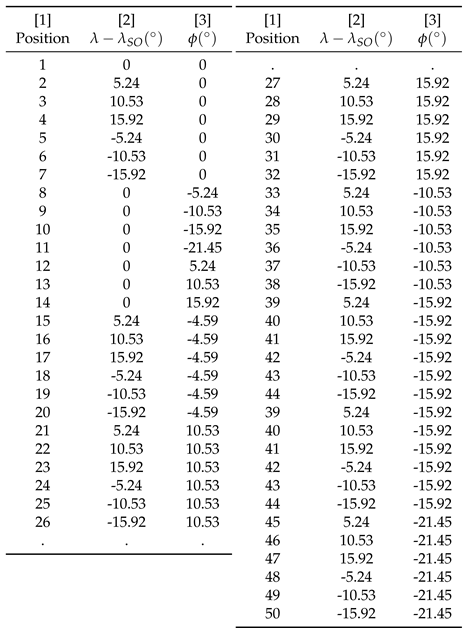

Table 2.
Scanning sequences for Jupiter VLT/ESPRESSO observing run on 21/22 July 2019.
| [1] | [2] | [3] | [4] |
| Seq. Number | Location | Time-Interval (UT) | Position Order |
| (1) | Equator | 00:18 - 01:02 | 1-5-6-7-1-2-3-4 |
| (2) | S Lat 10 | 01:06 - 02:28 | 9-36-33-34-1-37-38 |
| (3) | N Lat 10 | 02:33 - 03:01 | 1-13-24-25-21-22 |
| (4) | N Lat 15 | 03:05 - 03:17 | 14-31-28 |
| (5) | S Lat 15 | 03:20 - 03:43 | 1-42-43-39-10 |
| (6) | S Lat 15-20 | 03:47 - 04:20 | 48-49-45-46-11-40 |
[1] sequence number; [2] location on disk; [3] Time Interval of the beginning and end of sequence (in UT); [4] Points acquisition order. All positions were observed twice with a 60 second exposure each.
Table 3.
Pointing geometry for VLT/ESPRESSO observations of Jupiter on July 2019.
[1] Point nomenclature (also present in Figure 1); [2] planetocentric longitude of point relative to sub-observer meridian (sub-terrestrial in this case); [3] Latitude of the point’s center.
3. Doppler Velocimetry with VLT/ESPRESSO
Here we describe the adaptation of our Doppler velocimetry method to the case of Jupiter. This technique already proof to be highly effective and precise in the study of Venus atmosphere’s dynamics and in the retrieval of wind measurements based on high-resolution spectra observations [13,34,35,36,54]. Contrary to the cloud-tracking technique where we gather averaged winds over a set time interval (determined by the temporal distance between the two images in the pair) for large cloud structures, since the minimum size of features is directly reliant on image resolution, the Doppler velocimetry method provides instantaneous wind velocity measurements using Fraunhofer lines (characteristic absorption lines from gas in the Sun’s photosphere when interacting with continuum radiation emitted from warmer and deeper layers of our host star) in the visible part of the spectrum scattered by cloud particles of the target atmosphere (in our case Jupiter). The Doppler shifts manifested in the Fraunhofer lines of the back-scattered sunlight from particles in the atmosphere, which move with some relative velocity with respect to our frame of reference are used to compute instantaneous velocity values of particles in the atmosphere [54].
3.1. Projected Radial Velocities
Although the Doppler velocimetry technique is thoroughly described in Machado [35], Machado [36] and Goncalves [13], for the case of Venus atmospheric studies using the high-resolution spectrographs ESPaDOnS/CFHT and HARPS-N/TNG, we describe it again here for clarity reasons and since the adaptation of the Doppler velocimetry method for the case of ESPRESSO/VLT observations of Jupiter is here done for the first time. One of the great challenges pertaining ground-based observations of planetary winds lies in maintaining a stable velocity reference when acquiring data. Several different techniques that use high-resolution spectroscopy to retrieve planetary winds in the visible part of the spectrum have all addressed this issue [5,13,32,33,34,35,36,53,54]. The reason for this challenge is that radiation dispersion laws and inherent instrumental uncertainties have constrained absolute reference rest frames with accuracies no better than about 100 m/s to measure winds directly, while global winds on most planetary targets, while substantially different, can have wind amplitude variations or latitudinal gradients on the order of 5-10 m/s projected on the line-of-sight. However, with the recent instruments such as HARPS and ESPRESSO, primarily used for exoplanet search and characterisation, we can retrieve wind velocities with extreme precision, lower than 5-10 m/s. The Doppler velocimetry method used in this work is based on an optimal weighting of the Doppler shifts of all the lines present in the spectrum, relative to some reference spectrum.
This is accomplished by performing a weighted average of all the lines in the Fraunhofer spectrum using the inverse of the variance as a weighting factor:
where the weighting factor is the inverse of each individual line contribution to the variance. To consider this we must assume that the representative noise when gathering
The Doppler shift present in the lines of the solar backscattered spectrum results from two instantaneous motions. One motion is between the Sun and Jupiter’s upper cloud particles whose Doppler shift is minimal near the planet’s sub-solar point and maximum at the sub-terrestrial point (observer). Another is between the observer and the planet’s atmosphere, resulting from the topocentric velocity of cloud particles in the target’s atmosphere in the observer’s reference frame whose Doppler shift reaches its lowest value close to the sub-terrestrial point and highest at the sub-solar point. These combined motions add-up and contribute to a spatial variation of the Doppler shift as a function of latitude and longitude on the target. If is the phase angle between the Sun and Earth centred on the target, at Half Phase Angle (HPA) the sum of both Doppler shifts from the two instantaneous motions is zero.
A diagram for these two motions is illustrated in Figure 2. This is important since through this situation we always have a null-Doppler shift meridian assuming a purely zonal wind field. Hence, it can serve as a reference point and also a tool to measure any kind of spurious Doppler shifts that come from either additional wind components or sources other than the particles’ velocity. This effect has been taken advantage of by using the whole null-Doppler meridian to study any shift present in the spectra of back-scattered solar radiation on Venus at this location, which is presumed to be the result of meridional wind flow [13]. Since solar radiation is scattered from both Jupiter and Earth’s atmospheres and taking into account that some Fraunhofer lines are absorbed by our atmosphere, the contribution from telluric lines needs to be accounted for. To this end, the instrument registers both spectra and a least-squares deconvolution is applied to the pattern of Fraunhofer lines, using a mask that matches the Sun’s stellar type (G2 type star), providing the radial velocity (along the line-of-sight) in the solar system barycentric frame (B). From the correlation function between Fraunhofer lines scattered from Jupiter and Earth, a double Gaussian fit is applied to extract the velocity h of the radiation scattered off of the target only. However, to calculate this velocity other components are introduced to account for additional contributions to the Doppler shifts of the lines and it is necessary to express these measurements in Jupiter’s centre (of mass) rest frame:
where is the radial component of the instantaneous velocity of the planet’s clouds in the observer’s direction expressed in the centre rest frame of the target (P), h is the absolute velocity of solar lines scattered off the planet’s clouds expressed in the barycentric frame (B), is the correction from Earth’s rotation and orbital motion, i.e. the observer’s movement in the barycentric frame (B), is the instantaneous velocity of the planet’s centre of mass in the topocentric frame (T), and is the contribution of the Doppler shift from the differential rotation of the planet. The values for the velocities and are taken from the ephemerides calculated by an online platform hosted by JPL/NASA (https://ssd.jpl.nasa.gov/horizons.cgi). Contrary to previous works [13,15,34,35,36,37], the planet’s rapid rotation contributes with a non-negligible influence in the measured Doppler shifts. For this purpose we used the standard rotation velocities from the System III [43] for the gas giant, which give it a spin velocity at equator of approximately 12.6 km/s.
Due to the extended angular size of the Sun as seen from Jupiter () and its fast rotation (∼2 km/s) a differential elevation of the finite solar disk near the terminator leads to an imbalance between the contribution of the approaching (blue shifted radiation) and receding (red shifted radiation) solar limbs. In this geometric configuration, the excess of one or the other has an effect on the apparent line Doppler shifts measured on the planet’s atmosphere. This phenomenon is called the “Young effect”, first noticed by [56] and its implications on Doppler velocimetry methods in [12]. Although it can be relevant for other targets within the Solar system, the Young effect, when calculated for Jupiter has an influence of less than 0.1 m/s, which is minor when compared with the expected wind velocities in Jupiter (100-150 m/s).
3.1.1. De-projection coefficients
The velocities retrieved through the Doppler shift from Eq. 2 are radial velocities, thus they are projected along the line-of-sight. To obtain the amplitude of the wind velocities on the planet at each point observed in the planetocentric frame of reference we need to compute the local de-projection factor (F).
where is the phase angle at which the observation was performed, is longitude of the point being measured on the disk and is the latitude of the sub-terrestrial point. This factor is modulated by both the geometry of observations and the planetary longitude as seen from the ground. In the case of a zonal circulation, as what is evaluated here, the line-of-sight Doppler shift is proportional to the projection of wind velocity on the bisector phase angle [34]. For each location probed on the disk of Jupiter as illustrated in Figure 1, these coefficients were calculated and then used to convert the extracted Doppler shifts to instantaneous velocities of particles in the atmosphere.
3.1.2. Instrumental spectral drift
The spectral acquisition of Jupiter’s bands by VLT/ESPRESSO is sequential, thus monitoring possible changes in spectral calibration with time is required to ensure measurement robustness. When the instantaneous velocity of the planet’s centre of mass () is subtracted from the calculated velocity of atmospheric particles with the Doppler shift on the spectra retrieved, spectral wavelength calibration is performed at both the beginning and end of the observing session. In this case, this calibration was performed with a Th-Ar lamp exposure. Since the absorption lines from Earth’s atmosphere are well known, their superposition to the target planet’s spectra can be used as additional on-sky calibration.
As mentioned earlier, global wind circulation is on most planets such as Jupiter, subject to wind amplitude variations or latitudinal gradients that can range between 5 to 40 m/s projected on the line-of-sight. Even though ESPRESSO is already capable of a good enough spectral resolution, which can take into account such deviations with direct measurements, we have taken from previous experience [13,15,35,36,37] that better results can be achieved by measuring relative Doppler shifts between two sets of absorption lines. Choosing arbitrarily the first spectrum of each series of sequential acquisitions as a velocity reference so that:
where represents the line-of-sight relative velocity, which results from the subtraction of the absolute velocity retrieved at some target point in the planet’s disk () and the velocity in the reference point. With each return to the point of reference, a slow drift of the velocity retrieved from this point becomes apparent, which presumably occurs due to imperfectly corrected instrumental effects and measurement of absorption lines from the Sun with respect to those from the Earth [53]. Since to calculate relative Doppler shifts we use a reference point during observations, this point is returned to several times to correct the velocities retrieved from the instrumental spectral drift and/or spectral calibration variability with time. The reference point chosen is located in the meeting point between the equator and the HPA meridian so that theoretically both meridional and zonal components (respectively) of the winds gathered from the Doppler shifts should be null. Such properties makes this point the ideal reference for the spectral drift by making several observations during sequence acquisition.
Since we assume that any variations of the Doppler shift measured on this reference point come from the spectral drift provoked by the instrument, we fit all the reference point velocities to a series of linear segments , taking the initial velocity from the reference point to have a zero offset. With this trend line, it is possible to compute the offset caused by the spectral drift at any point in time during observations, which is then used to further correct the velocities retrieved:
where each relative Doppler retrieval is subtracted by the value of the drift trend at the time was observed, obtaining the spectral drift corrected velocity .
3.1.3. Error Estimation
The total error on a given velocity measurement is the sum of several uncertainties which have different origins. The spectral calibration performed using the Th-Ar lamp can be subject to uncertainties regarding the dispersion spectrum from the lamp itself, the least-square deconvolution of Fraunhofer lines, the additional fit to telluric lines and unpredictability of weather conditions as well as minor variations in temperature and pressure of the spectrograph, and guiding and pointing accuracy can all have uncertainties, which affect the Doppler shifts measured that will be used to compute the velocity of winds on Jupiter. Since the referenced multiple sources have errors of varying degree and we repeat exposures on the same point in the disk as part of our observing routine, it is possible to test the internal consistency of the retrieved radial velocity (h) instead of estimating upper limits for each source of error. An estimate of the individual error on each velocity retrieved was made by calculating the standard deviation between two 60 second exposures for each point. Depending on the instrument and the observing time available, more exposures are usually preferred to ensure the consistency of the acquisition process. The velocities on each target point were obtained by weight-averaging the retrieved values from consecutive exposures. Taking as the error on the reference point velocity relative to the retrieval , the statistical combined error for each point can be calculated using:
where represents the linearly interpolated error from the deviations of from along the segment between two reference point exposures. The errors calculated for our Doppler velocimetry measurements with ESPRESSO, taking into account all the factors considered above were on average 10.6 m/s with the largest error bar being around 19.3 m/s. Even though all previously mentioned sources of error are important for the precision of the results obtained with this method, the error associated with the pointing accuracy of the fibre’s FOV during an exposure was at least one order of magnitude higher than all other contributors to the general error, since this error will be propagated through the de-projection of line-of-sight drifts into wind velocities of both zonal and meridional components. To monitor these fluctuations, the observer has the responsibility to control the fibre’s FOV drift, verifying if it wanders by more than half the fibre’s angular diameter from the targeted point. Should it do so, the observation is discarded and then repeated, a process that is limited by the total allocated time for the observation with the telescope. For the case of ESPRESSO two 60 second exposures were enough to guarantee a good S/N ratio, while the stability of this state-of-the-art instrument allowed such exposures to be made with confidence.
4. Results
4.1. Doppler winds with VLT/ESPRESSO
The results presented in this section constitute a first-time retrieval of atmospheric winds in Solar System planets by ESPRESSO. Thus, given the exploratory nature of this work, we regard these as the first step to fine-tune our model of observation and techniques for the next generation of instruments and telescopes.
With our observing strategy and posterior data reduction and corrections we were able to retrieve multiple longitudinal profiles of the zonal component of the winds in Jupiter at selected bands signaling the distinct flow regimes.
The changing zonal flow direction and magnitude on equatorial latitudes (20N - 20S) is readily apparent with our results in Table 4. The values presented form an average of the Doppler winds retrieved at each latitude band.
Figure 3 shows the wind velocity values retrieved along each band for each position observed with ESPRESSO. For this observing run, the winds are stable within the error bars of the retrieved data however, at the 10 we see increased variability in the same latitudinal band.
5. Comparison with previous measurements
5.1. Cloud Tracking
Given the general stability of the zonal wind profile of Jupiter, we can compare our Doppler velocimetry retrievals with previous results, even if observations are separated by a number of years. However, some caution must be taken since, although the general variability of the wind profile stays on the order of 10 m/s, which is comparable to our error bars, episodes of increased variability have been observed [1]. The magnitude of the jets at approximately 7S and 6N, and 24 has been noticed to change by more than 40 m/s at specific periods of observation [2,11,22].
The general stability of the zonal wind profile of Jupiter can be verified in Figure 4. This plot also highlights the periods of variability at specific regions on Jupiter’s banded circulation. Several authors have explored the causes for these changes [1,10,50], mentioning that the time intervals for these variations can range from hours to months, making it difficult to determine the average zonal wind profile and the exact culprit of many of these changes [1]. For all measurements in Figure 4, a cloud tracking method was employed even if several techniques from individual [10] and automatic tracking [44] to 2D correlation routines [6,9] were used.
We can see our Doppler velocimetry results compared with retrieved wind velocities from different instruments in Figure 5. The Cassini profiles feature reference data from automatic cloud tracking from two separate authors [42,44], and an additional analysis using 2D correlation of mosaics built with Cassini/ISS images during the fly-by period between December and January 2000/2001 [9]. For completion we present an additional wind profile with cloud tracking results using a semi-automatic method, on which we targeted similar latitudes that were observed with ESPRESSO. Even though the data from this cloud-tracking routine is approximately 20 years apart from our Doppler wind retrievals, such a comparison is still useful to evaluate the profile’s evolution through time.
The middle panel feature more profiles due to the higher cadence of observations provided by HST, including an effort to continuously provide imaging data on Jupiter’s atmosphere to accompany its evolving atmosphere, through the OPAL program which started observations in 2014 [55] on Uranus and 2015 on Jupiter [47]. The record of HST observations in Figure 5 starts in 1995 with the study by [10] who did not report any significant changes to zonal wind profile during their period of observation. The next set of observation occur with [11] which couples observations with both Cassini and HST in 2008, reporting an increase on the 6N jet by approximately 40 m/s. We include then a more extensive report of HST observations in [50] featuring Hubble data from 2009-2016 and another observation in 2016 by [18] which was accompanied by ground-based observations. The last set of data from 2017 was explored in [22], who also analysed the zonal wind profile of Jupiter with different filters from HST.
The rightmost panel in Figure 5 shows ground based measurements taken from observations with the Pic du Midi 1 meter telescope [2] and a collection of different observations from Amateur astronomers and PlanetCam UPV/EHU [46] mounted on the 2.2 meter telescope in Calar Alto Observatory [18].
From the three profiles we can verify that there is reasonable agreement between our Doppler retrievals and previous results however, it is interesting to note that at the equator, the Doppler winds appear to be faster than any previous measurements, by a difference that exceeds 20 m/s, double what local and temporal variations to the zonal wind predict. It is possible that this value is an outlier but, given the exploratory nature of this work, and thus lack of more substantial data, it is difficult to confirm this.
5.2. Previous Doppler Velocimetry results
Since this work explores the capabilities of ESPRESSO to perform Doppler velocimetry on planetary atmospheres of the Solar System, the volume of data of this kind to compare with our observations is relatively scarce as opposed to cloud tracking. Multiple studies [14,15,34,35,36,37] have used Doppler velocimetry to retrieve winds on Venus at visible wavelengths and other targets have been considered with similar techniques such as Mars at submm/mm wavelengths [29,38] and Titan in the infrared range [24,25,26,27].
Doppler velocimetry on Jupiter at similar wavelengths than this work was achieved with success for the first time in [13] with JOVIAL-JIVE (Jovian Oscillations through Velocity Images At several Longitudes - Jovian Interiors from Velocimetry Experiment in New Mexico) observations in 2015 and 2016.
A comparison between the Doppler winds retrieved for this work and previous measurements with a similar technique are presented in Figure 6. Even though both techniques use visible solar light reflected on Jupiter’s upper tropospheric clouds, and the time separation between observations is not large when looking at previous comparisons with cloud-tracked winds, there is some discrepancy between both data sets. Although there is good agreement at 10S and 15S, our other average values differ from the profiles retrieved by [13] by 5-6 (the error bar of our retrievals) when taking into account the other data points. Since this method measures the actual velocity of atmospheric particles, Doppler winds can be subject to variations due to wave activity [13], which can translate to higher magnitude differences than the previously mentioned 10 m/s. However, when comparing our results with observations with HST in 2015, 2016 (see Figure 5) which [13] have used for comparison in their Doppler velocimetry results, we do not find such significant differences. It is true that this work is exploratory and it features a single observing run, but ESPRESSO has an overall higher spectral resolution than the instrument used in [13], which can be an alternate explanation, as ESPRESSO results should be more sensitive to the alternating jets of Jupiter.
5.3. Multiwavelength Comparison
Since ESPRESSO observations, for the purpose of this work, were performed using the full set of Fraunhofer lines in the visible part of the spectrum, it is possible that the winds retrieved with our Doppler method originate from different regions of the troposphere than the visible cloud layer observed with previously with Cassini or HST. In [22], they employ a multiwavelength analysis of Jupiter’s banded structure, to study the zonal wind profile’s variation as function of wavelength.
In Figure 7 we present the zonal wind profile at multiwavelengths in both ultraviolet [30] and visible wavelengths [22] to compare with our Doppler results. The profile remains mostly unchanged at visible wavelengths (395-658 nm), except at the two most powerful jets at approximately 7S and 23N which seem more sensitive to different wavelengths. Also, most cloud features that are identified with cloud-tracking techniques are present on most visible wavelength filters with little changes to morphology or drift rate [30], hence the stability of the zonal wind profile across several wavelengths is also in part a consequence of the relatively large vertical structure of most tracked features. The wind profile retrieved in the ultraviolet (264 nm) tracked features that could not be observed at other wavelengths similar to the ones discussed in [22]. These higher winds at approximately 350 mbar pressure level [52] appear to have less prominent jets across all latitudes and a slight increase in wind magnitude at the equator. However, it is not enough to justify the 110 m/s Doppler wind retrieved at the equator with ESPRESSO.
Longitudinal variations could also explain some of these differences between the results presented in this work and the legacy of zonal wind measurements retrieved, as these can have magnitudes that go beyond the standard deviation of our results as reported in [22].
5.3.1. Considerations on Altitude of Wind Velocity Tracers
Even though wind results from both our Doppler technique and cloud-tracking seem consistent, there are important differences in how these velocities are retrieved. This can have implications on their interpretation and vertical location in the atmosphere [37]. The cloud-tracking method follows the movement of cloud features in the atmosphere. As such, the altitude/pressure level from which winds are extracted is directly dependent on where these features are formed and propagate, which for the case of Jupiter is roughly at the 0.7-1.5 bar level [45,52]. The Doppler velocimetry method used in this work relies on back-scattered sunlight dispersed from Jupiter’s atmosphere. The spectra obtained by ground-based observers is the result of a bolometric integration of this back-scattered radiation towards the observing line-of-sight. Although mostly concentrated on the region where optical depth reaches unity, which is roughly where the cloud features can form in the upper troposphere [1,42], it is possible that the average radiation that arrives at the instrument’s detector could include scattering from slightly higher levels. For this reason, it is reasonable to expect some fluctuations in the results from both techniques. A more extensive observing campaign of Jupiter with high resolution spectroscopy, coupled with coordinated observations to perform cloud tracking in a multiwavelength range would allow further exploration of this subject.
Since the Doppler velocimetry method relies on solar light back-scattered from Jupiter’s dayside atmosphere, the altitude of the retrieved zonal velocities ought to be located where the optical depth reaches unity [37]. Several models for the cloud properties on each band have been developed over the years which applied to the bands observed in this study show that optical thickness unity is reached in the Equatorial Zone at approximately 0.7 bar, and to slightly deeper values for both the North and South Equatorial Belts [3,7,48]. According to these models, we can be sensing somewhere between the upper part of the cloud layer and a chromophore coating, postulated by [4] to explain the red colouring of Jupiter’s Great Red Spot and then expanded by [49] to explain the different colourations of the belts. From this contrast between belts and zones, it is possible that features followed with cloud-tracking could be formed at different pressure levels. Although this is out of the scope of this exploratory study, since with our Doppler velocimetry technique we use observations in the visible wavelength range, it is possible that we might be sensing slightly different pressure levels as a function of wavelength. We intend to address this issues in our follow up research.
5.4. Wind component entanglement
Since we are measuring winds from the radial velocity component obtained from back scattered spectra of Jupiter, the resulting wind velocity is the sum of all its components. This method has been used extensively to study Venus [14,15,34,35,36,37] where the zonal wind dominates atmospheric circulation at the cloud tops. For the case of Jupiter, each band can be understood as its own Hadley cell to the point that globally, meridional circulation is generally not measurable from Earth due to low spatial resolution [12]. The presence of storms, particularly in the belts, along with a high level of turbulence is evidence of vigorous convection and vertical wind shear in the upper troposphere of Jupiter, which means that the vertical component of wind velocity could be an important contributor to the overall wind velocity retrieved from the Doppler velocimetry method. Hence, there is the possibility that our method is sensitive to additional components of the wind. However, since this study covered a small region over a short time interval in the atmosphere of Jupiter, and consequently few data points, it is challenging to evaluate the strength of the vertical wind contribution from these results alone.
6. Conclusions
In this body of work, we have attempted to explore the capabilities of VLT/ESPRESSO in the study of Solar System planets atmospheres, in this case Jupiter. We have adapted and refined a Doppler velocimetry method to retrieve wind velocities on the upper atmosphere of Jupiter from ground-based telescopes, with heritage from observations of Venus made with different instruments [13,15,34,35,36,37]. This exploratory project has shown evidence that Doppler velocimetry applied to visible spectra from back-scattered solar radiation from the atmosphere of Jupiter is efficient to retrieve wind velocity results along Jupiter’s different latitudinal bands. To support this new application of the method we compared our retrieved Doppler winds with the ones obtained from the analysis of Cassini images of Jupiter taken during its fly-by manoeuvre in December 2000 using the cloud tracking technique (CT). However, winds derived in this manner (CT) are usually averaged over several days of observations and do not reflect instantaneous wind velocity and its significant variability at shorter time scales. The ground-based Doppler velocimetry technique has proven its reliability in constraining global wind circulation models, complementary of space-based measurements, we also assessed the feasibility of monitoring Jupiter’s atmosphere dynamics and variability on short time scales, from the ground. This work also shows that we can take advantage of ground-based observations, with the extremely high-resolution spectroscopic capabilities of VLT/ESPRESSO, for studying the spatial wind variability of winds and the presence of storms on Jupiter troposphere.
In spite of the limited spatial and temporal coverage of Jupiter’s disk allowed by the allocated observations, our results show general consistency between both techniques applied here to Jupiter, this agreement is mostly clear when we compare the latitudinal averaged wind profile as we presented before. Furthermore, results from both cloud-tracking and Doppler velocimetry are also consistent with reference results from various papers that represent a diverse study of the upper troposphere of Jupiter with different instruments from Cassini and HST [18,42].
Given that pointing accuracy is the most important source of error for Doppler wind results, there is the possibility that the ESPRESSO observations are skewed by a few arc seconds which in some cases might be enough to alter significantly the wind measurements retrieved due to the steep wind velocity difference between some bands and also the fact that some of these latitudes stand at the cusp between zones and belts. Although seeing conditions during the observing run were optimal (1.25 maximum), it might be enough to influence pointing accuracy at the scale of belt/zone transitions [12].
Since this study shows clearly that the Doppler velocimetry technique, using high-resolution spectroscopy and ground-based observations, is effective to perform dynamical atmospheric studies on Jupiter, and despite the aforementioned consistency between the results with other techniques using space-based observations, we do see slight fluctuations in some of bands studied with both methods and provided several tentative hypotheses for their origin however, given the exploratory nature of this work, our coverage was limited thus no firm conclusions could be made regarding the differences in wind velocities retrieved between both methods. With the observed general agreement between the results, we intend to perform in the future a wider observational study to cover a broader region of Jupiter with the possibility to analyse more elements of the banded structure of its atmosphere and greater temporal coverage, possibly observing Jupiter over several days, not only to extract winds during a full rotation period but also to investigate temporal daily variability.
Since we sense the overall visible wavelength range with the Doppler velocimetry technique and since optical depth is a function of wavelength, it is possible to explore the use of partial wavelength ranges in order to sense, at the same time, different pressure levels/altitudes simultaneously. To confirm the location of pressure levels probed with such a study, we plan to employ a modern radiative transfer suite, such as NEMESIS [20]. Such observations, coupled with cloud-tracking results, could allows us to estimate the vertical shear of the zonal wind in the upper troposphere where a transition between circulation regimes might be occurring [8].
Author Contributions
Conceptualization, P.M and J.S.; Data Curation, J.S, P.M., R.G., F.B., J.R. and M.S.; Formal analysis, P.M, J.S. and R.G.; investigation, P.M., J.S. and M.S.; methodology, P.M., J.S. and R.G.; visualization, J.S., P.M., R.G. and F.B.; validation, P.M. and J.S.; writing—original draft preparation, J.S.; writing—review and editing, P.M and J.S.; supervision, P.M.; observations, P.M. and R.G. All authors have read and agreed to the published version of the manuscript.
Funding
This research was funded by the Portuguese Fundação Para a Ciência e Tecnologia under project P-TUGA Ref. PTDC/FIS-AST/29942/2017 through national funds and by FEDER through COMPETE 2020 (Ref. POCI-01-0145 FEDER-007672). J.S. also acknowledges the funding by the University of Lisbon through the BD2017 program based on the regulation of investigation grants of the University of Lisbon, approved by law 89/2014, the Faculty of Sciences of the University of Lisbon
Data Availability Statement
Data available in a publicly accessible repository. The data presented in this study are openly available in Machado, Pedro (2023), “Dataset23_Jupiter_PMachado”, Mendeley Data, V1, doi: 10.17632/7smfyv5y53.1.
Acknowledgments
We acknowledge the support from the University of Lisbon through the BD2017 program based on the regulation of investigation grants of the University of Lisbon, approved by law 89/2014, the Faculty of Sciences of the University of Lisbon and the Portuguese Foundation for Science and Technology (FCT) through the project P-TUGA with the code PTDC/FIS-AST/29942/2017. We give credit to the full team behind the Cassini-Huygens space mission and the ISS instrument for availability of the data archive used for this research. We also acknowledge the full support by all personnel behind VLT and ESPRESSO which made the acquisition of data fro Doppler velocimetry possible. This study was based on observations collected at the European Organisation for Astronomical Research in the Southern Hemisphere under ESO program 0103.C-0203(A). F.B. acknowledges the support by an FCT grant with the reference: 2021.05455.BD and and J.R. for the fellowship grant 373 2021.04584.BD
Conflicts of Interest
The authors declare no conflict of interest.
References
- Asay-Davis, X.S.; Marcus, P.S.; Wong, M.H.; de Pater, I. Changes in Jupiter’s zonal velocity between 1979 and 2008. Icarus 2010, 211, 1215–1232. [Google Scholar] [CrossRef]
- Barrado-Izagirre, N.; Rojas, R.; Hueso, R.; Sánchez-Lavega, A.; Colas, F.; Dauvergne, J.L.; Peach, D. IOPW Team, Jupiter’s zonal winds and their variability studied with small-sized telescopes. A&A 2013, 554, A74. [Google Scholar] [CrossRef]
- Braude, A.S.; Irwin, P.J.; Orton, G.S.; Fletcher, L.N. Colour and Tropospheric Cloud Structure of Jupiter from MUSE/VLT: Retrieving a Universal Chromophore. Icarus 2020, 338, 113589. [Google Scholar] [CrossRef]
- Carlson, R.W.; Baines, K.H.; Anderson, M.S.; Filacchione, G.; Simon, A.A. Chromophores from photolyzed ammonia reacting with acetylene: Application to Jupiter’s Great Red Spot. Icarus 2016, 274, 106–115. [Google Scholar] [CrossRef]
- Civeit, T.; Appourchaux, T.; Lebreton, J.P.; Luz, D.; Courtin, R.; Neiner, C.; Witasse, O.; Gautier, D. On measuring planetary winds using high-resolution spectroscopy in visible wavelengths. A&A 2005, 431, 1157–1166. [Google Scholar] [CrossRef]
- Choi, D.S.; Showman, A.P. Power spectral analysis of Jupiter’s clouds and kinetic energy from Cassini. Icarus 2011, 216, 597–609. [Google Scholar] [CrossRef]
- Dahl, E.K.; Chanover, N.J.; Orton, G.S.; Baines, K.H.; Sinclair, J.A.; Voelz, D.G.; Wijerathna, E.A.; Strycker, P.D.; Irwin, P.J. Vertical structure and color of Jovian latitudinal cloud bands during the Juno Era. arXiv 2020, arXiv:2012.06740. [Google Scholar] [CrossRef]
- Fletcher, L.N.; Kaspi, Y.; Guillot, T.; Showman, A.P. How Well Do We Understand the Belt/Zone Circulation of Giant Planet Atmospheres. Space Sci. Rev. 2020, 216, 30. [Google Scholar] [CrossRef]
- Galperin, B.; Young, R.M.B.; Sukoriansky, S.; Dikovskaya, N.; Read, P.L.; Lancaster, A.J.; Armstrong, D. Cassini observations reveal a regime of zonostrophic macroturbulence on Jupiter. Icarus 2014, 229, 295–320. [Google Scholar] [CrossRef]
- García-Melendo, E.; Sánchez-Lavega, A. A study of the stability of Jovian zonal winds from HST images: 1995-2000. Icarus 2001, 152, 316–330. [Google Scholar] [CrossRef]
- García-Melendo, E.; Arregi, J.; Rojas, J.F.; Hueso, R.; Barrado-Izagirre, N.; Gómez-Forrellad, J.M.; Pérez-Hoyos, S.; Sanz-Requena, J.F.; Sánchez-Lavega, A. Dynamics of Jupiter’s equatorial region at cloud top level from Cassini and HST images. Icarus 2011, 211, 1242–1257. [Google Scholar] [CrossRef]
- Gaulme, P.; Schmider, F.X.; Goncalves, I. Measuring planetary atmospheric dynamics with Doppler spectroscopy. A&A 2018, 617, A41. [Google Scholar] [CrossRef]
- Gonçalves, I.; Schmider, F.X.; Gaulme, P.; Morales-Juberías, R.; Guillot, T.; Rivet, J.; Appourchaux, T.; Boumier, P.; Jackiewicz, J.; Sato, B. First measurements of Jupiter’s zonal winds with visible imaging spectroscopy. Icarus 2019, 319, 795–811. [Google Scholar] [CrossRef]
- Goncalves, R.; Machado, P.; Widemann, T.; Peralta, J.; Watanabe, S.; Yamazaki, A.; Satoh, T.; Takagi, M.; Ogohara, K.; Lee, Y.-J. Venus’ cloud top wind study: Coordinated Akatsuk/UVI with cloud tracking and TNG/HARPS-N with Doppler velocimetry observations. Icarus 2020, 335, 113418. [Google Scholar] [CrossRef]
- Goncalves, R.; Machado, P.; Widemann, T.; Brasil, F.; Ribeiro, J. A wind study of Venus’ cloud top: New Doppler velocimetry observations. Atmosphere 2021, 12, 2. [Google Scholar] [CrossRef]
- Hansen, C.J.; Caplinger, M.A.; Ingersoll, A.; Ravine, M.A.; Jensen, E.; Bolton, S.; Orton, G. Junocam: Juno’s outreach camera. Spc. Sci. Rev. 2017, 243, 475–506. [Google Scholar] [CrossRef]
- Hueso, R.; Legarreta, J.; Rojas, J.F.; Peralta, J.; Pérez-Hoyos, S.; del Río-Gaztelurrutia, T.; Sánchez-Lavega, A. The Planetary Laboratory for Image Analysis. Adv. Space Res. 2010, 46, 1120–1138. [Google Scholar] [CrossRef]
- Hueso, R.; Sánchez-Lavega, A.; Iñurrigarro, P.; Rojas, J.F.; Pérez-Hoyos, S.; Mendikoa, I.; Gómez-Forrellad, J.M.; Go, C.; Peach, D.; Colas, F.; Vedovato, M. Jupiter cloud morphology and zonal winds from ground-based observations before and during Juno’s first perijove Geophys. Res. Lett. 2017, 44, 4669–4678. [Google Scholar] [CrossRef]
- Hueso, R.; Sánchez-Lavega, A.; Rojas, J.F.; Simon, A.A.; Barry, T.; Río-Gaztelurrutia, T.; Antuñano, A.; Sayanagi, K.M.; Delcroix, M.; Fletcher, L.N. Saturn atmospheric dynamics one year after Cassini. Icarus 2020, 336, 113429. [Google Scholar] [CrossRef]
- Irwin, P.C.J.; Teanby, N.A.; de Kok, R.; Fletcher, L.N.; Howett, C.J.A.; Tsang, C.C.C.; Wilson, C.F.; Calcutt, S.B.; Nixon, C.A.; Parrish, P.D. The NEMESIS planetary atmosphere radiative transfer and retrieval tool. Journal of Qt. Spec & Rad. Transfer 2008, 109, 1136–1150. [Google Scholar] [CrossRef]
- Irwin, P. Giant Planets of Our Solar System, 2nd ed.; Springer-Praxis: Chichester, UK, 2009. [Google Scholar]
- Johnson, P.E.; Juberías-Morales, R.; Simon, A.; Gaulme, P.; Wong, M.H.; Cosentino, R.G. Longitudinal variability in Jupiter’s zonal winds derived from multi-wavelength HST observations. Planetary and Space Science 2018, 155, 2–11. [Google Scholar] [CrossRef]
- Kaspi, Y.; Galanti, E.; Hubbard, W.B.; Stevenson, D.J.; Bolton, S.J.; Iess, L.; Guillot, T.; Bloxham, J.; Connerney, P.; Cao, H. Jupiter’s atmospheric jet streams extend thousands of kilometres deep. Nature Lett 2018, 555, 223–226. [Google Scholar] [CrossRef] [PubMed]
- Kostiuk, T.; Fast, K.; Livengood, T.; Hewagama, T.; Goldstein, J.; Espenak, F.; Buhl, D. Direct measurement of winds on Titan Geophys. Res. Lett. 2001, 28, 2361–2364. [Google Scholar] [CrossRef]
- Kostiuk, T.; Livengood, T.; Hewagama, T.; Sonnabend, G.; Fast, K.; Murakawa, K.; Tokunaga, A.; Annen, J.; Buhl, D.; Schmulling, F. Titan’s stratospheric zonal wind, temperature, and ethane abundance a year prior to Huygens insertion Geophys. Res. Lett. 2005, 32, L22205. [Google Scholar] [CrossRef]
- Kostiuk, T.; Livengood, T.; Sonnabend, G.; Fast, K.; Hewagama, T.; Murakawa, K.; Tokunaga, A.; Annen, J.; Buhl, D.; Schmulling, F.; et al. Stratospheric global winds on Titan at the time of Huygens descent Jrn. Geophys. Res.: Planets 2006, 111, E7. [Google Scholar] [CrossRef]
- Kostiuk, T.; Hewagama, T.; Fast, K.; Livengood, T.; Annen, J.; Buhl, D.; Sonnabend, G.; Schmulling, F.; Delgado, J.; Achterberg, R. High spectral resolution infrared studies of Titan: Winds, temperature, and composition Planet. Spa. Sci. 2010, 58, 1715–1723. [Google Scholar] [CrossRef]
- Lebreton, J.P.; Matson, L. An Overview of the Cassini mission. Il Nuovo Cimento 1992, 15, 1137–1147. [Google Scholar] [CrossRef]
- Lellouch, E.; Goldstein, J.; Bougher, S.; Gabriel, P.; Rosenqvist, J. First absolute wind measurements in the middle atmosphere of Mars Astrophys. J. 1991, 383, 401. [Google Scholar] [CrossRef]
- Li, L.; Ingersoll, A.; Vasavada, A.; Simon-Miller, A.; Del Genio, A.; Ewald, S.; Porco, C.; West, R. Vertical wind shear on Jupiter from Cassini images Jrn. Geophys. Res. 2006, 111, E04004. [Google Scholar] [CrossRef]
- Limaye, S.S. Jupiter: New estimates of the mean zonal flow at the cloud level. Icarus 1986, 65, 335–352. [Google Scholar] [CrossRef]
- Luz, D.; Civeit, T.; Courtin, R.; Lebreton, J.-P.; Gautier, D.; Rannou, P.; Kaufer, A.; Witasse, O.; Lara, L.; Ferri, F. Characterization of zonal winds in the stratosphere of Titan with UVES. Icarus 2005, 179, 497–510. [Google Scholar] [CrossRef]
- Luz, D.; Civeit, T.; Courtin, R.; Lebreton, J.-P.; Gautier, D.; Witasse, O.; Kaufer, A.; Ferri, F.; Lara, L.; Livengood, T. Characterization of zonal winds in the stratosphere of Titan with UVES: 2. Observations coordinated with the Huygens Probe entry. Jour. Geophys. Res. 2006, 111, E08S90. [Google Scholar] [CrossRef]
- Machado, P.; Luz, D.; Widemann, T.; Lellouch, E.; Witasse, O. Mapping zonal winds at Venus’s cloud tops from ground-based Doppler velocimetry. Icarus 2012, 221, 248–261. [Google Scholar] [CrossRef]
- Machado, P.; Widemann, T.; Luz, D.; Peralta, J. Wind circulation regimes at Venus’ cloud tops: Ground-based Doppler velocimetry using CFHT/ESPaDOnS and comparison with simultaneous cloud tracking measurements using VEx/VIRTIS in February 2011. Icarus 2014, 243, 249–263. [Google Scholar] [CrossRef]
- Machado, P.; Widemann, T.; Peralta, J.; Goncalves, R.; Donati, J.-F.; Luz, D. Venus cloud-tracked and doppler velocimetry winds from CFHT/ESPaDOnS and Venus Express/VIRTIS in April 2014. Icarus 2017, 285, 8–26. [Google Scholar] [CrossRef]
- Machado, P.; Widemann, T.; Peralta, J.; Gilli, G.; Espadinha, D.; Silva, J.E.; Brasil, F.; Ribeiro, J.; Goncalves, R. Venus Atmospheric Dynamics at Two Altitudes: Akatsuki and Venus Express Cloud Tracking, Ground-Based Doppler Observations and Comparison with Modelling. Atmosphere 2021, 12, 506. [Google Scholar] [CrossRef]
- Moreno, R.; Lellouch, E.; Forget, F.; Encrenaz, T.; Guilloteau, S.; Millour, E. Wind measurements in Mars’ middle atmosphere: IRAM Plateau de Bure interferometric CO observations. Icarus 2009, 201, 549–563. [Google Scholar] [CrossRef]
- Mousis, O.; Hueso, R.; Beaulieu, J.-P.; Bouley, S.; Carry, B.; Colas, F.; Klotz, A.; Pellier, C.; Petit, J.-M.; Rousselot, P.; et al. Intrumental method for professional and amateur collaborations in planetary astronomy Exp. Astron. 2014, 38, 91–191. [Google Scholar] [CrossRef]
- Pepe, F.; Molaro, P.; Cristiani, S.; Rebolo, R.; Santos, N.C.; Dekker, H.; Mégevand, D.; Zerbi, F.M.; Cabral, A.; Di Marcantonio, P.; et al. ESPRESSO: The next European exoplanet hunter. Astron Nachr 2014, 335, 10–22. [Google Scholar]
- Pepe, F.; Cristiani, S.; Rebolo, R.; Santos, N.C.; Dekker, H.; Cabral, A.; Di Marcantonio, P.; Figueira, P.; Lo Curto, G.; Lovis, C.; et al. ESPRESSO@VLT - On-sky performance and first results. A&A 2021, 645, A96. [Google Scholar] [CrossRef]
- Porco, C.C.; West, R.; McEwen, A.; Del Genio, A.D.; Ingersoll, A.P.; Thomas, P.; Squyres, S.; Dones, L.; Murray, C.D.; Johnson, T.V. Cassini Imaging of Jupiter’s Atmosphere, Satellites, and Rings. Science 2003, 299, 1541. [Google Scholar] [CrossRef] [PubMed]
- Riddle, A.; Warwick, J. Redefinition of System III longitude. Icarus 1976, 27, 457–459. [Google Scholar] [CrossRef]
- Salyk, C.; Ingersoll, A.P.; Lorre, J.; Vasavada, A.; Del Genio, A.D. Interaction between eddies and mean flow in Jupiter’s atmosphere: Analysis of Cassini imaging data. Icarus 2006, 185, 430–442. [Google Scholar] [CrossRef]
- Sánchez-Lavega, A. Introduction to Planetary Atmospheres, 1st ed.; CRC Press, Taylor & Francis group: Boca Raton, 2011. [Google Scholar]
- Sánchez-Lavega, A.; Rojas, J.; Hueso, R.; Perez-Hoyos, S.; Bilbao, L.; Murga, G.; Ariño, J. PlanetCam UPV/EHU: a simultaneous visible and near infrared lucky-imaging camera to study solar system objects. Ground-based and Airborne Instrumentation for Astronomy IV. In Proceedings of the SPIE, 2012, 8446.
- Simon, A.A.; Wong, M.; Orton, G. First results from the Hubble OPAL program: Jupiter in 2015. The Astrophys. J. 2015, 812, 8. [Google Scholar] [CrossRef]
- Simon-Miller, A.A.; Banfield, D.; Gierasch, P.J. Color and the Vertical Structure in Jupiter’s Belts, Zones and Weather Systems. Icarus 2001, 154, 459–474. [Google Scholar] [CrossRef]
- Sromovsky, L.A.; Baines, K.H.; Fry, P.M.; Carlson, R.W. A possibly universal red chromophore for modeling color variations on Jupiter. Icarus 2017, 291, 232–244. [Google Scholar] [CrossRef]
- Tollefson, J.; Wong, M.H.; de Pater, I.; Simon, A.A.; Orton, G.S.; Rogers, J.H.; Atreya, S.K.; Cosentino, R.G.; Januszewski, W.; Morales-Juberías, R.; et al. Changes in Jupiter’s zonal wind profile preceding and during the Juno mission. Icarus 2017, 296, 163–178. [Google Scholar] [CrossRef]
- Vasavada, A.R.; Ingersoll, A.P.; Banfield, D.; Bell, M.; Gierasch, P.J.; Belton, M.J.S.; Orton, G.S.; Klaasen, K.P.; DeJong, E.; Breneman, H.H.; et al. Galileo imaging of Jupiter’s atmosphere: the great red spot, equatorial region, and white ovals. Icarus 1998, 135, 265–275. [Google Scholar] [CrossRef]
- West, R.A.; Baines, K.H.; Friedson, A.J.; Banfield, D.; Ragent, B.; Taylor, F.W. Jovian clouds and hazes. In Jupiter: the planet, satellites and magnetosphere; Bagenal, F., Dowling, T., McKinnon, W., Eds.; Cambridge University Press, 2007; p. 79. [Google Scholar]
- Widemann, T.; Lellouch, E.; Campargue, A. New wind measurements in Venus’ lower mesosphere from visible spectroscopy Planet. Space Sci. 2007, 55, 1741–1756. [Google Scholar] [CrossRef]
- Widemann, T.; Lellouch, E.; Donati, J.-F. Venus Doppler winds at cloud tops observed with ESPaDOnS at CFHT Planet. Space Sci. 2008, 56, 1320–1334. [Google Scholar] [CrossRef]
- Wong, M.; Simon, A.; Orton, G.; Pater, I.; Sayanagi, K. Hubble’s long-term OPAL (Outer Planet Atmospheres Legacy) program observes cloud activity on Uranus 46th Lunar and Planetary Science Conference 2015, The Woodlands, Texas, p. 2606, LPI Contribution No. 1832.
- Young, A. Is the Four-Day “rotation” of Venus illusory? Icarus 1975, 24, 1–10. [Google Scholar] [CrossRef]
Figure 1.
Schematic of the observing routine on Jupiter by VLT/ESPRESSO on the 22nd of July 2019. The small circles represent the FOV of the fibre proportional to the size of Jupiter’s disk in the context of these observations (0.5 arc seconds in diameter for the size of the FOV). We also included a grid to tentatively map the relative position of each observing position in latitude and longitude. Grid lines have intervals of 15 on both coordinates. The solid black line on the right side of the spherical grid represents the morning terminator while the blue dotted line marks the location of the 12 h local time meridian. The picture of the planet’s disk was taken from the Planetary Virtual Observatory and Laboratory. Picture credits go to Gary Walker.
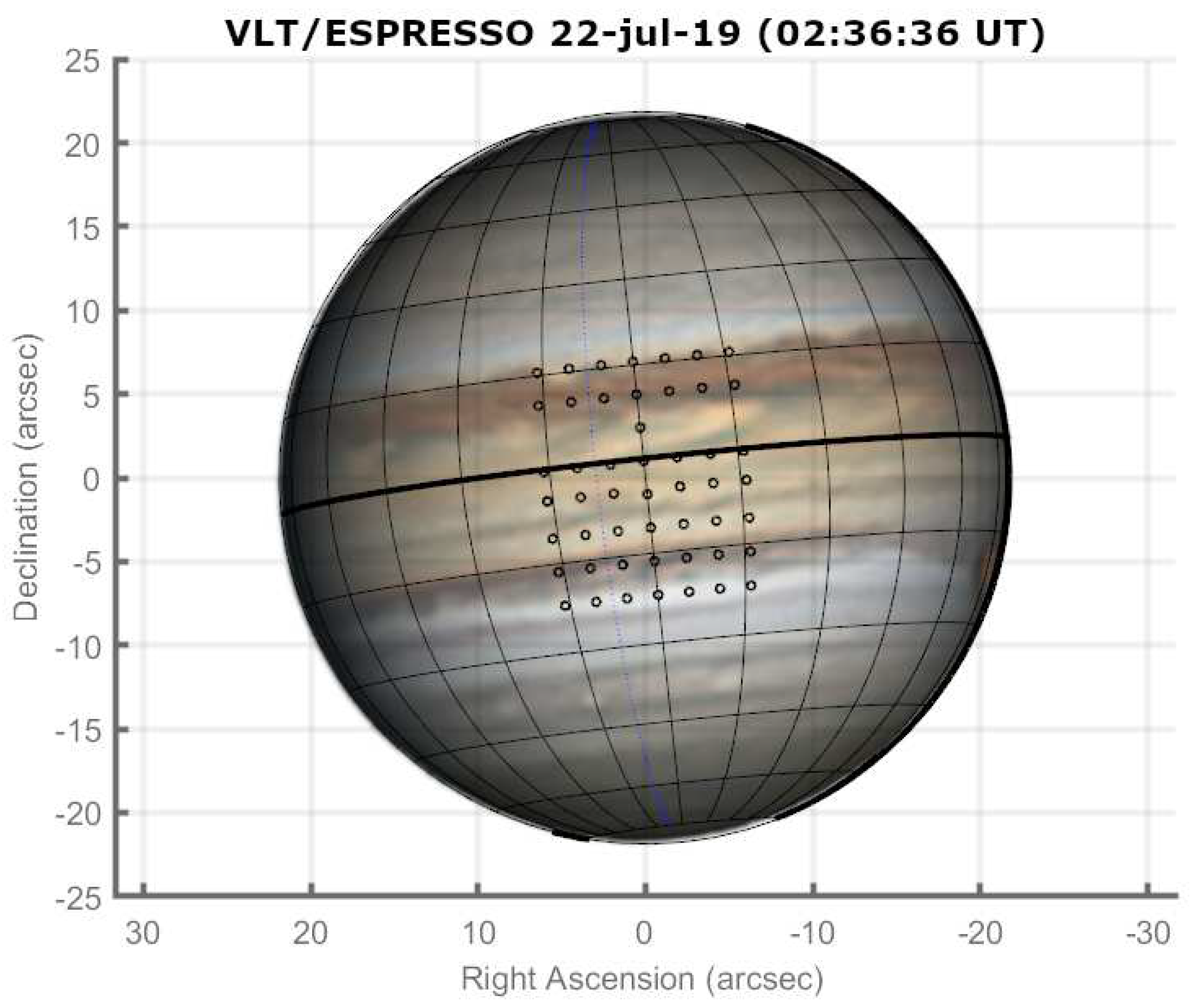
Figure 2.
Diagram of the Doppler effect on backscattered solar radiation from particles on Jupiter. This model assumes a single scattering approximation. The solid white arrows represent radiation being absorbed (right) and then emitted (left) without Doppler effect. The coloured arrows represent the respective Doppler shifts provoked by the relative movements of particles with respect to Earth when radiation is absorbed (red) or emitted (blue) by them. is the phase angle between the Sun and Earth, centred on the planet.
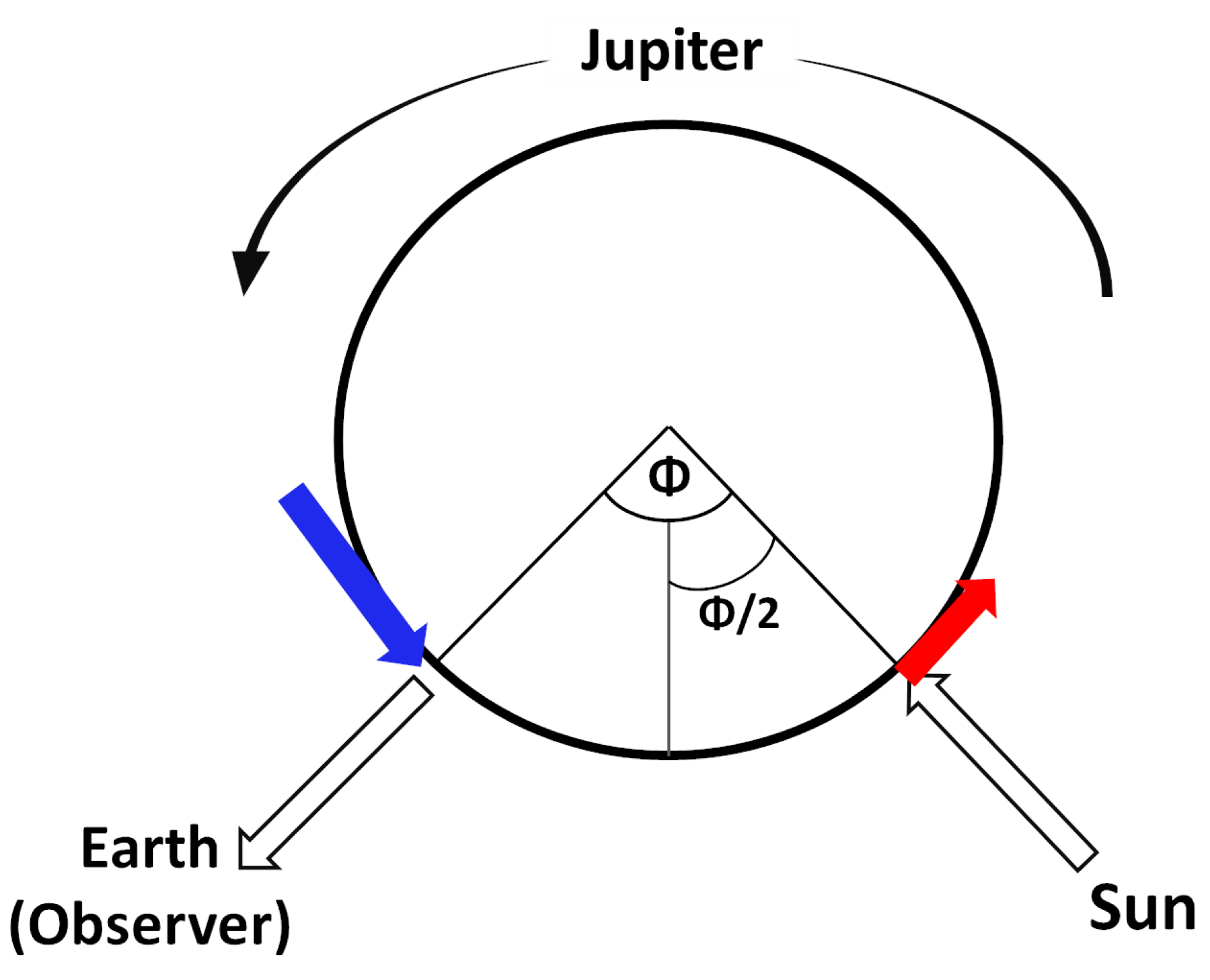
Figure 3.
Longitudinal profiles of the zonal wind in each band of Jupiter with observations from VLT/ESPRESSO. The longitude in these plots has the sub-observer longitude as the reference point, hence it is not the true planetary longitude.
Figure 3.
Longitudinal profiles of the zonal wind in each band of Jupiter with observations from VLT/ESPRESSO. The longitude in these plots has the sub-observer longitude as the reference point, hence it is not the true planetary longitude.
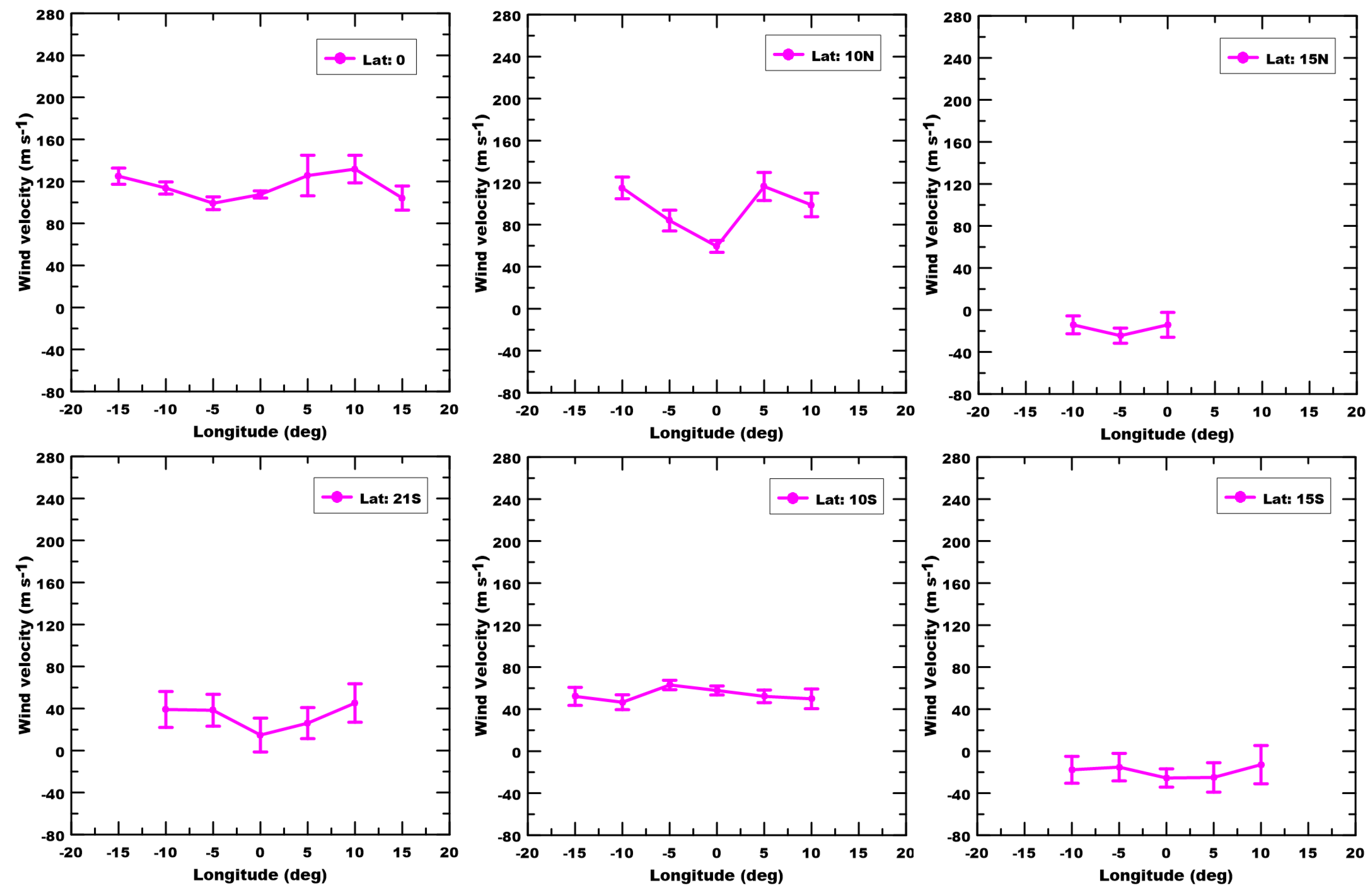
Figure 4.
The zonal wind profile of Jupiter’s upper tropospheric clouds at approximately 0.7-1.5 bar. The different profiles concern observations throughout approximately two decades taken with Cassini during its fly-by manoeuvre in December 2000 [9], ground observations at Pic-du-Midi [2] and HST [10,11,22,50]. The winds represented here were retrieved with cloud tracking techniques.
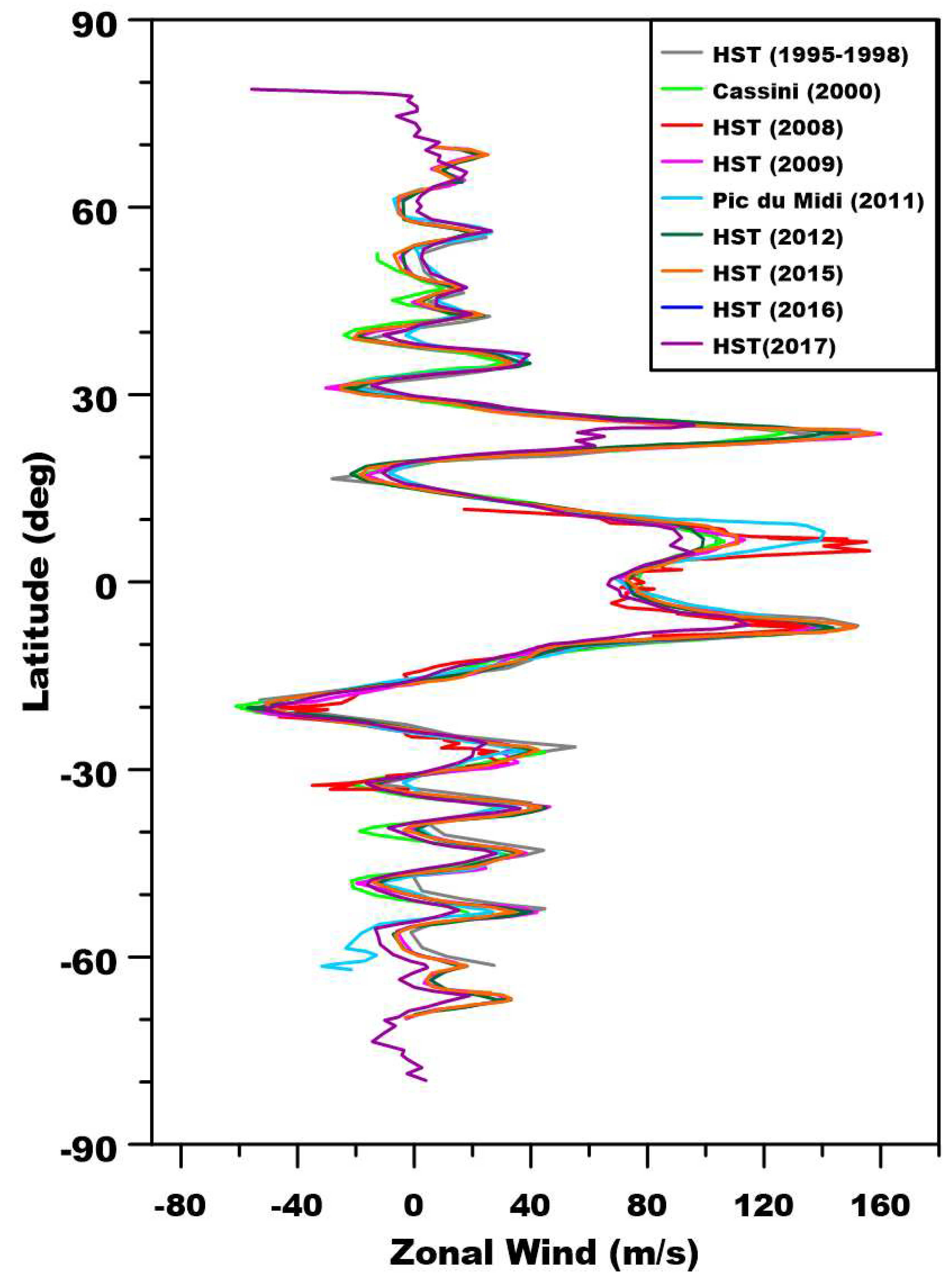
Figure 5.
Comparative wind profiles retrieved from Cassini, HST and ground based observations with Doppler velocimetry results at visible wavelengths. We limit the profiles to equatorial latitudes to match the range of our ESPRESSO observations. Each of the wind profiles used for comparison is taken from a previous publications with the exception of the red profile in the leftmost panel. These are wind velocity results retrieved with 2D Semi-Automatic Correlation cloud-tracking using the PLIA tool [17].
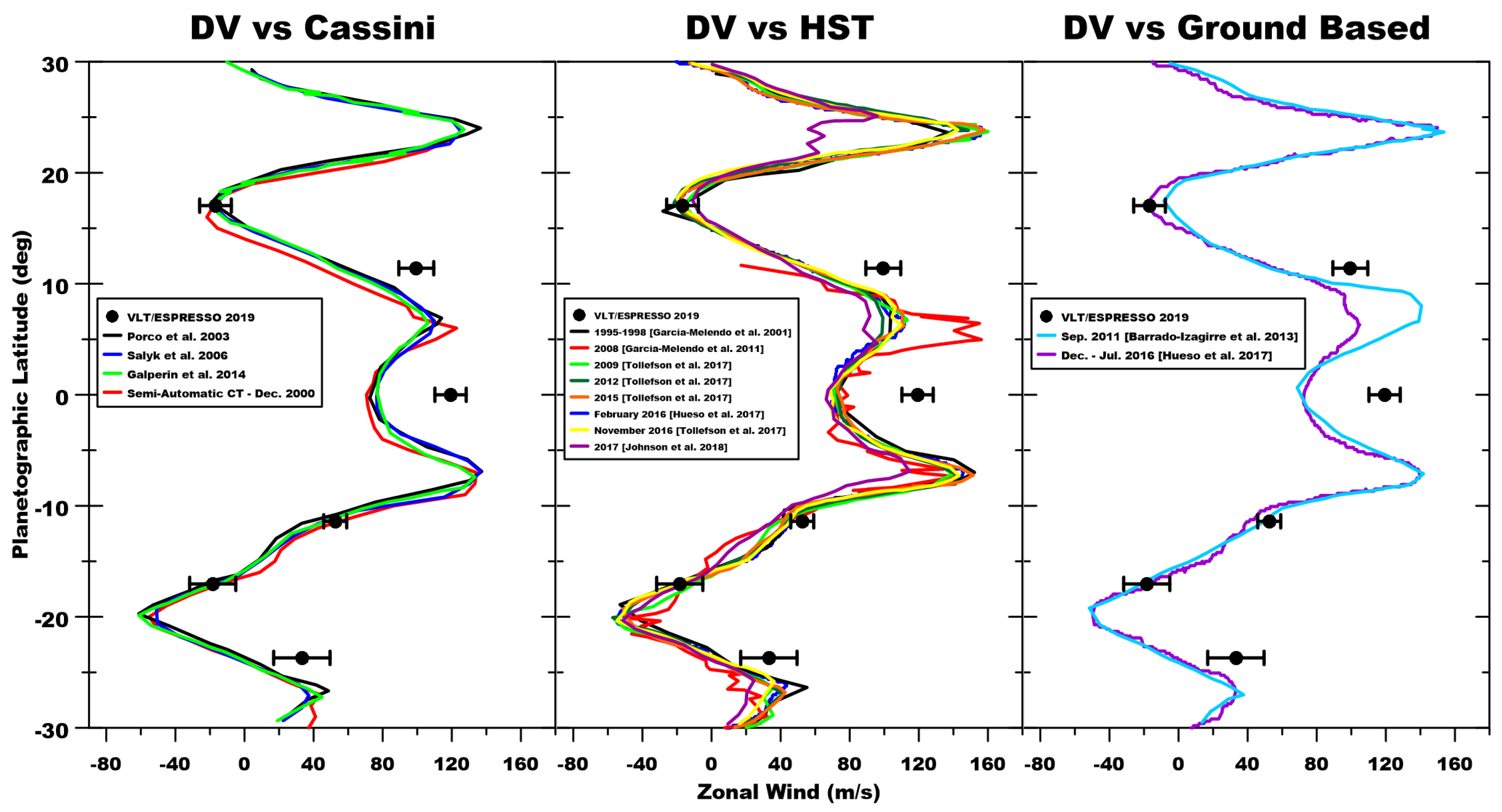
Figure 6.
Zonal winds retrieved with Doppler velocimetry techniques with VLT/ESPRESSO observations (calculated average - black crosses) and the JOVIAL-JIVE retrievals in 2015 (blue profile) and 2016 (red profile). The faint gray circles are the data points of our Doppler wind retrievals from which the average was calculated, whose values are presented in Table 4.
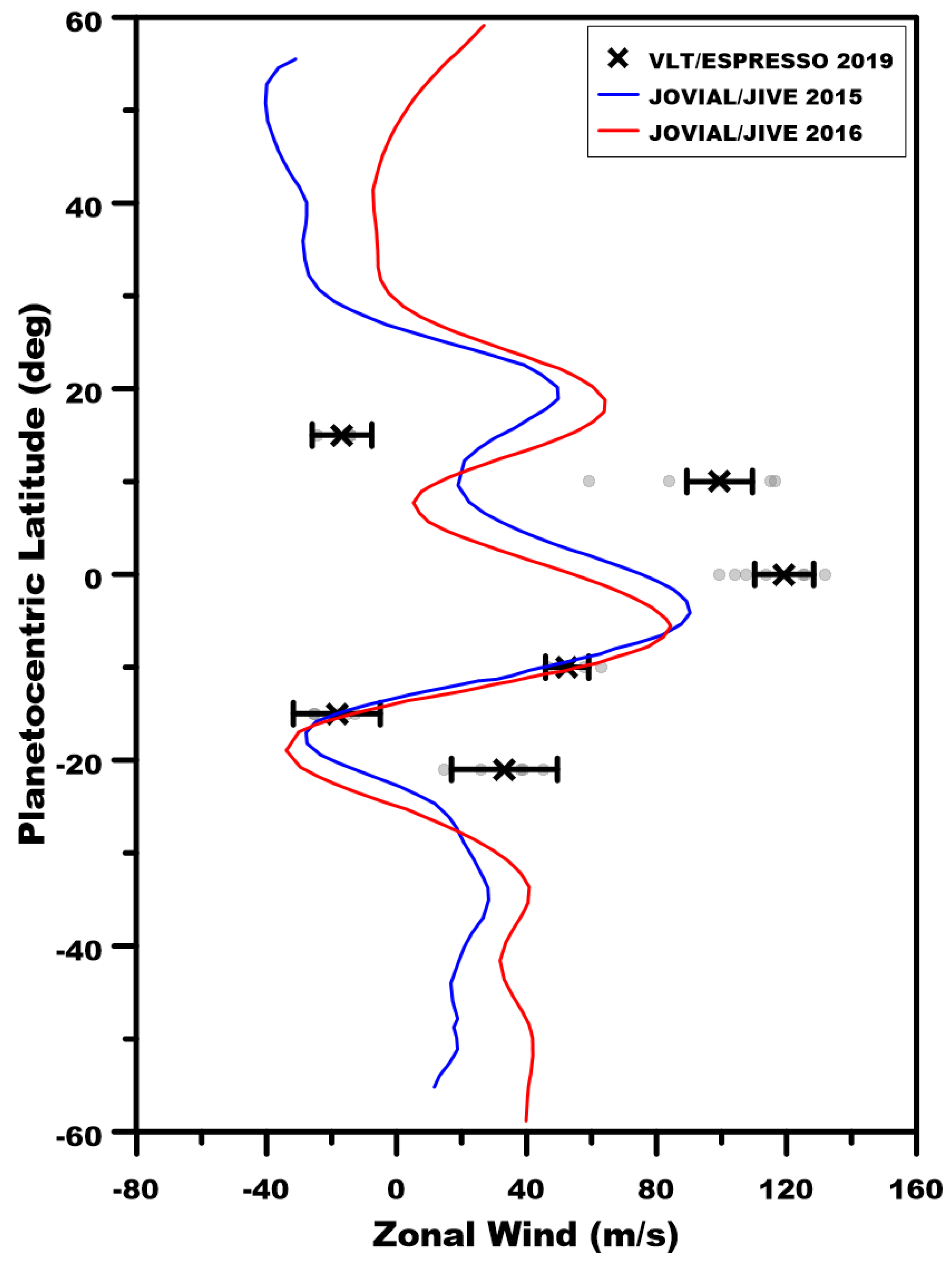
Figure 7.
A multiwavelength analysis of the zonal wind profile on Jupiter at visible and ultraviolet wavelengths to compare with the Doppler winds retrieved with VLT/ESPRESSO. The ultraviolet profile from [30] is the result of cloud tracking of higher altitude features than what is identified at visible wavelengths at 0.7-1.5 bar. The other five profiles were all retrieved with HST observations as described in [22].
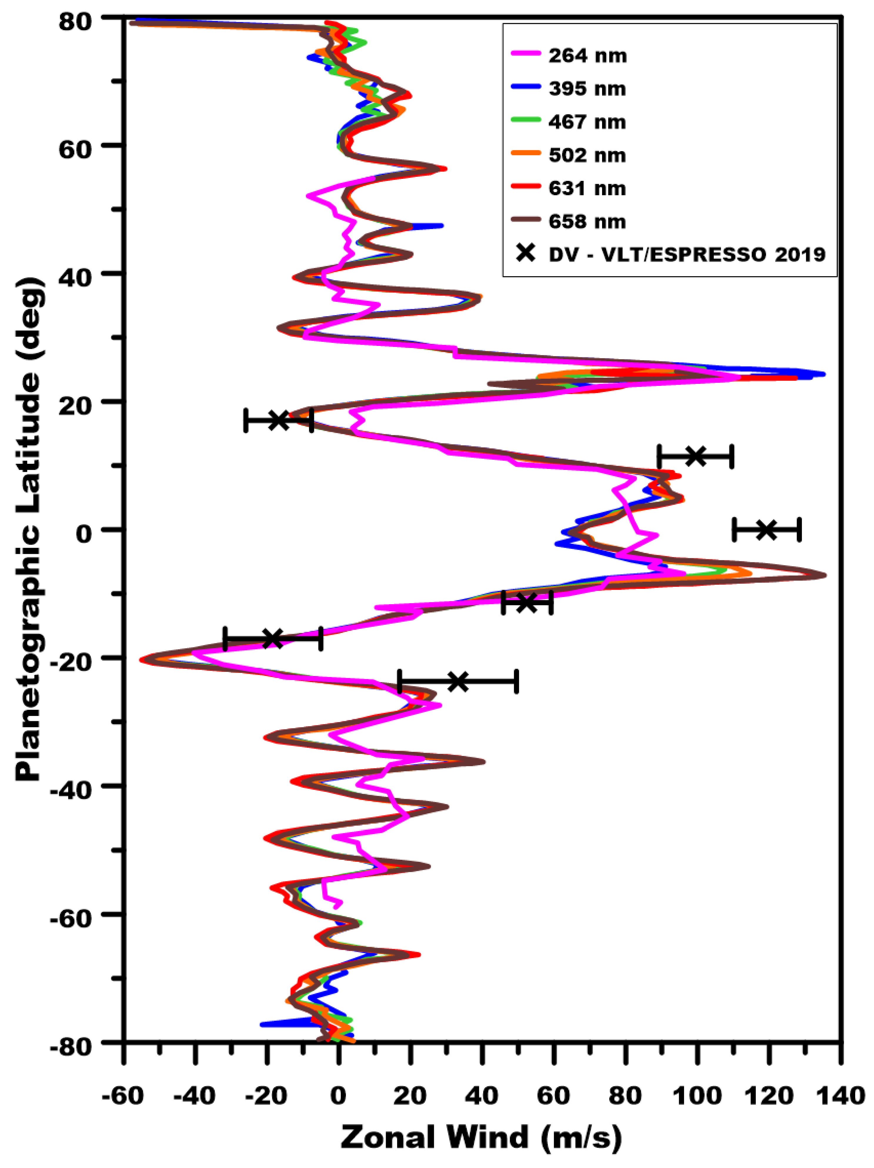
Table 1.
Summary of target characteristics during ESPRESSO observations of Jupiter
| (1) | (2) | (3) | (4) | (5) | (6) |
| Date | Time (UT) | () | Ang.Diam.(") | Sub-Obs.Lat () | Air-mass |
| 21/22 July | 23:03 - 04:20 | 7.7 | 45.92 | -3.05 | 1.003 - 1.254 |
The Date and Time-Interval refer to the value registered by the instrument during observations; (3) is the Phase Angle; (4) is the size of the disk of Jupiter in the sky in arc seconds; (5) is the sub-observer latitude on Jupiter’s frame; and (6) represents the air-mass at the target’s location in the sky during observations.
Table 4.
Averaged Doppler winds on each latitude band observed with VLT/ESPRESSO
| [1] | [2] | [3] |
| Latitude () | Doppler Wind (m.s) | Error (m.s) |
| 0 | 119.30 | 9.07 |
| 10 | 99.43 | 10.1 |
| -10 | 52.49 | 6.65 |
| 15 | -16.8 | 9.17 |
| -15 | -18.4 | 13.36 |
| -21 | 33.2 | 16.3 |
[1] Observed latitude band; [2] Zonal wind speed calculated from Doppler Velocimetry technique; [3] Average error of measurements in its corresponding latitudinal band. Negative values of the zonal wind indicate westward flow.
Disclaimer/Publisher’s Note: The statements, opinions and data contained in all publications are solely those of the individual author(s) and contributor(s) and not of MDPI and/or the editor(s). MDPI and/or the editor(s) disclaim responsibility for any injury to people or property resulting from any ideas, methods, instructions or products referred to in the content. |
© 2023 by the authors. Licensee MDPI, Basel, Switzerland. This article is an open access article distributed under the terms and conditions of the Creative Commons Attribution (CC BY) license (http://creativecommons.org/licenses/by/4.0/).
Copyright: This open access article is published under a Creative Commons CC BY 4.0 license, which permit the free download, distribution, and reuse, provided that the author and preprint are cited in any reuse.


