
Submitted:
08 December 2023
Posted:
08 December 2023
You are already at the latest version
Abstract
In this research, 117,718 ionospheric perturbations, with a space size (t) of 20–300 s but no limit on amplitude (A) have been automatically searched globally by a software from ion density data measured by the DEMETER satellite for more than 6 years. The influence of the solar activity on the ionosphere has been firstly examined and the results have presented that the solar activities can globally enhance ionospheric irregularities but rarely induce plasma variations more than 100%. A statistical work has been performed on ion PERs to check their dependence on local time and it is shown that there are 24.8% perturbations appeared in daytime (10:30 LT) and 75.2% ones in nighttime (22:30 LT). Ionospheric fluctuations with an absolute amplitude A < 10% tend to be background variations and the percentages of positive perturbations with small A < 20% are 64% in daytime and 26.8% in nighttime, respectively, but this number is revers for mid-large amplitude PERs. There is a demarcation point in space size t = 120 s and occurrence probabilities of day PERs are always higher than that of nighttime ones before this point while this trend is contrary after this point. Distributions of PER according to various amplitudes or space scales have been characterized by typical seasonal variations either in daytime or in nighttime. The EIA only exists in dayside equinox and winter occupying two lowlatitude crests with lower Np. The huge WSA appears in all periods except for dayside summer full of PERs with enhanced amplitude, especially in winter night. The WN-like structure can be obviously figured out in all seasons showing absolutely space large-scales. In the meanwhile, several magnetic anomalous zones of planetary scale non-dipole fields, such as the SAMA, Northern Africa anomaly, and so on, have been also successfully detected by extreme negative ion perturbations in this time.
Keywords:
Ionospheric Structures
; Ion Perturbations
; Automatic detection method
1. Introduction
As a conductive part of layers of the atmosphere, investigations on the various properties of the ionosphere have been always a hot issue under controversial due to its tremendous responses to natural and artificial events, such as natural hazards and communication engineering. As early as in 1930s, ionospheric irregularities caused by inhomogeneous ionization density in the topside ionosphere have been primarily described [1,2,3]. After several decades of research, ionospheric structures even their inner various features, have been gradually gained more and more clear configurations from ground-based remote ionospheric responding and satellite in-situ instruments [4,5,6,7]. Some of them like the equatorial ionization anomaly (EIA) and mid-latitude ionospheric trough (MIT) have been well reconstructed by different parameters although part of potential mechanisms of these various ionospheric irregularities are still on the way of understandings [8,9,10,11,12].
Plasma density is the primary parameter that is usually utilized to reconstruct the ionosphere configuration and testify the reliability of measuring data from different instruments. Electron density (Ne) is the key parameters to characterize the status of ionospheric plasma and the O+ is the main ion among the ions although it depends on some factors, such as, local time, altitude, and so on [13,14,15,16]. Electron density measured on in-situ DEMETER (Detection of Electro-Magnetic Emissions Transmitted from Earthquake Regions)and Swarm satellites or from FORMOSAT-3/COSMIC radio occultation measurements has been employed to investigate the properties of ionospheric irregularities such as EIA, MIT, middle latitudinal band structures, Wedell Sea Anomaly, and so on [11,17,18,19,20,21,22]. Other parameters like O+, H+ and He+ densities and total electron density are also used to research ionospheric characteristics of background, seasonal and day-to-day variations and large-scale depletion of oxygen ion [23,24,25].
At the same time, as the development of the Earth’s observation from space, more and more evidences have been presented that the ionosphere could be unexpectedly sensitive to seismic activities and seismo-ionospheric influence has been generally acted as a most prospective candidate for earthquake forecasting and seismogenic electromagnetic energy transmitting among lithosphere, atmosphere, ionosphere and even magnetosphere [26,27,28,29,30,31]. However, it must be mentioned that variations of ionospheric parameters are not only due to earthquakes but also to other sources such as solar activity, acoustic gravity waves (AGW), travelling ionospheric disturbances, plasma dynamics, large meteorological phenomena [32]. As a weak factor of strong ionospheric background variations, faint information associated with seismic activities are always submerged in other enhanced irregularities. Aside from case study in a relative small region and specified short time, statistical investigations on seismo-ionospheric influence have always been a good way to distinguish anomalous features of earthquake precursors. Pulinits et al. have proposed that an earthquake with a magnitude 4.6 can theoretically induce ionospheric irregulars due to its effect scale keeping the same size as determined by the Dobrovolsky formula R = 100.43M, where R is the radius of earthquake preparation zone, and M is the earthquake magnitude [33,34]. Chen et al. have reported that the ionosphere shows anomalous fluctuations 1–5 days before 82% earthquakes with magnitudes more than 5 by calculating the relative variations of the median of the critical frequency of f0F2 [35]. There is a significant decrease 4 hours before strong earthquakes by comparing the power spectral densities of very-low frequency (VLF) electrical field measured in different periods of DEMETER life [36,37,38,39]. Liu et al. have presented that ionospheric anomalies on electron density tend to appear 11, 3, and 2 days prior to the M ≥ 6 events within 300 km using spatial analysis method [40].
With an alternative statistical method, Parrot [32] has correlated the DEMETER ion perturbations (PERs) automatically searched by software with strong earthquake events occurred during the DEMETER period and the results have shown that the number and the intensity of the ionospheric PERs are larger prior to earthquakes than prior to random events. Similar method has also utilized by Li et al. [41,42] to correlate ionospheric PERs measured by DEMETER satellite with strong seismic activities happening in corresponding period. They have found that the obtained results are not very good because not all ionospheric PERs are caused by EQs and the number of false alarms is large even the detected rang up to 1500 km. Further, Li et al. [43] have presented that CSES (China Seismo-Electromagnetic Satellite) ion PERs with space size of 200–300 s locate collectively in equatorial area with no specified correlation with the main seismic zones of the world. In the meanwhile, Li et al. [44] have found that there are different properties for ion PERs and electron ones obtained from CSES satellite for more than three years and ionospheric PERs with large amplitudes and large space sizes tend to collocate with large-scale ionospheric structures, such as EIA, MIT and so on.
Therefore, all evidences have indicated that it will be a great significance to explore ionospheric PERs caused by various interferences. A comprehensive investigation on properties of ionospheric PERs with different amplitudes and space sizes can help us understand well their producing mechanism and distinguish correctly earthquake precursors. So, in this paper, DEMETER data and data processing method are firstly introduced in Section 2. In Section 3, different seasonal and local time characteristics of ion PERs will be comparatively exhibited. Discussion and conclusions are in Section 4 and Section 5, respectively.
2. Data and data processing method
2.1. Dataset
DEMETER was launched in June 2004 measuring electromagnetic waves and plasma parameters all around the globe except in the auroral zones [45]. It is a low-orbit satellite with an altitude of 710 km, decreased to 660 km in December 2005. The orbit of DEMETER is nearly sun-synchronous and the upgoing and downgoing half-orbits correspond respectively to nighttime (22:30 LT) daytime (10:30 LT). Its payload IAP (plasma analyzer instrument) outputs plasma density of ion density with data resolutions of 4 s in survey mode and 2 s in burst mode for all data. This satellite’s science mission stopped measuring at the end of December 2010. More details can be referred to [45].
The investigation is based on the ion (O+) density (Ni) data from IAP on-board the DEMETER in-situ measurement more than 6 years (from August 2004 to November 2010). All data have been transmitted into the resolution of 4 s for ion density issued by the original recordings. At the same time, the SAVGOL method is employed to smooth the data eliminating pulse-like peaks before searching for PERs. The SAVGOL function returns the coefficients of a Savitzky-Golay smoothing filter [46].
2.2. Automatic search for ionospheric PERs
The plasma data processing method here is similar to the one used before by Li et al. [44]. Ionospheric PERs in ion dataset are automatically searched by a software globally rather than around worldwide the main seismic zones in our previous work [40,41]. Here, two key parameters are specified: the PER spatial scale (t, in-situ measurement time) is kept 20–300 s (140–2100 km if the satellite velocity 7 km/s is considered) and there are still no limits on the value of various amplitudes (A) in the PER database. The minimum size is also set to 20 s in order to to avoid spurious impulsions caused by one or two points [40]. Each ionospheric disturbance is described by several parameters, such as peak appearing time, orbit number, location (latitude and longitude), amplitude, spatial scale and so on. Eight three-hourly averaged Kp index values each day are available online: http://isgi.unistra.fr/data_download.php accessed on 1 October 2023 and the Kp value is also examined when each ionospheric PER detected happens.
As an example, the Kuril Islands M 8.3 earthquake occurred at 11.14.13 UT on November 15, 2006 with a depth of 10 km and a location (46.59°N, 153.27°E) (red star in Figure 1a), which magnetically conjugated point coordinates of 28.46°S and 147.82°E (blue star in Figure 1a) in the opposite hemisphere have been determined Using a magnetic field model. Figure 1a represents the orbit of 12545_1 (black line) measured by DEMETER which is close to this conjugate point (blue star) on November 12, 2006, i.e., 3 days before the EQ. The O+ density recorded along this orbit during night time is shown in Figure 1b with blue line (Data-ion) and its smoothed data using the SAVGOL function has been lined in red (Smo-ion).
Two ionospheric perturbations have been automatically detected in this Smo-ion line by the software with defined space size 20–300 s and without limit on their amplitudes. Their relative locations to the epicentre of the M 8.3 Kuril Islands EQ and its conjugated point have been shown in Figure 1a and their running configurations in the orbit data line have been exhibited in Figure 1b. The corresponding parameters of these two PERs have been presented in Table 1. It has been testified that the conjugated point of the epicentre of the M 8.3 Kuril Islands EQ locates in a near distance (38 km) to the PER1, which is considered seismo-ionospheric influence [47]. However, PER2 locates near the magnetic equator with a large space scale more than 2000 km and a large amplitude of 76.2%, which gains the probability that that this perturbation is attributed to EIA structure of the ionosphere. This point will also be illustrated in the following part of the paper.
Totally, there are 117,718 ion PERs attained form the ion density dataset during this period considered.
3. Different properties of ionospheric PERs
3.1. Effect of the solar activity on the ionosphere
As we all know, the solar activity gives a significant influence on the ionosphere either in daytime or in nighttime. So the Kp index has been firstly used here to examine the solar effect on the plasma densities. Figure 2 shows the distributions of all 117,718 ion PERs with an increasing value of corresponding Kp index as one PER occurred. From Figure 2, it is clear that the distributions of plasma variations in light of Kp index present no special areas, where PERs with large Kp values appear collectively although the solar activity tends to give a more heavier effect on equatorial and high latitude ionospheric areas: the effect from the magnetic storms are global [33,43,44,48].
To further examine exactly the influence of the solar activity on amplitude and space size of ionospheric PERs, firstly, PERs with Kp > 4 considered perturbed period and ones with Kp ≤ 2 for quiet period have been selected respectively from all 117,718 ion PERs to form two new groups of PERs: 87,057 with Kp ≤ 2 and 4,263 with Kp > 4. Secondly, for each group of PERs, the number for certain PERs (n, the same in the following parts) and their occurrence probability (p, the same in the following parts) have been calculated as a function of different ranges of amplitude (A): ≥100, 90–100, 80–90, 70–80, 60–70, 50–60, 40–50, 30–40, 20–30, 10–0, 0–-100, and <-100 and, space size (t): 20–40, 40–60, 60–80, 80–100, 100–120, 120–140, 140–160, 160–180, 180–200, and 200–300. The results have been listed into Table 2 and Table 3 with the number of each sub-group of PERs and their corresponding percentage in black.
From Table 2 and Figure 3a, considered percentage values corresponding to different scales of amplitude during magnetic storm (Kp > 4) and that in quiet period (Kp ≤ 2), on one hand, for positive PERs, the occurrence probabilities for plasma variations with a magnitude covering the range of 10% < A < 100% are 59.3% and 54.3%, 18.3% and 20.1% for ones 0–10%, but 12% and 13.8% for ones with magnitude more than 100% respectively for Kp > 4 and Kp ≤ 2. From this point, it is easy to infer that solar activities can enhance ionospheric variations but rarely induce plasma irregularities more than 100%. Large-scale ionospheric density enhancements are frequently observed during geomagnetic storms [49]. On the other hand, it is not easy for magnetic storms giving rise to negative ionospheric variations (See also Table 2 and Figure 3a).
In space scale, from Table 3 and Figure 3b, though the solar activity tends to induce ionospheric irregularities with relative large space sizes, for instance, t > 160 s, there is no obvious discrepancy between the space sizes of PERs appearing in disturbed period and quiet time, or, possibly due to magnetic storm inducing ionospheric variations with larger space sizes beyond what we have set here t = 20–300 s.
3.2. Local time discrepancy of ionospheric PERs
DEMETER measurement depends heavily on two local times of 22:30 LT in nighttime and 10:30 LT in the morning. For all 117,718 ion PERs, the number of ones occurred in daytime is 29,226 and 88,492 for nighttime, standing for 24.8% and 75.2%, respectively. To check the dependence of the occurrence of plasma PERs on local time, PERs for each parameter has been separated into two groups in the light of their occurrence time of daytime and nighttime. And then, for each group of PERs (day side or night side), the percentage for different ranges of amplitude A and different space size t have been calculated to form Table 4 and Table 5.
From Table 4 and Figure 4a, the percentages for all amplitude segments vary widely and this property shows more obviously in daytime. The significant feature is that plasma PERs with small amplitudes < 20% stand for a prominent proportion of 64% in day side. While this parameter only 26.8% in night side. The number of each group of PERs with an amplitude between 0 and -10% has also been checked: 3,406 and 5,603 for day and night ion PERs, standing respectively for 11.7% and 6.3% for all 29,226 day ion PERs and for 88,492 night ones. That means most of the ionospheric variations with positive and negative magnitude less than 10% tend to be background irregularities. This conclusion seems more right in nighttime than in daytime, when sunlight can speed ionization of plasma giving rise to more positive ionospheric irregularities. The occurrence probabilities of mid-large amplitude perturbations, for instance, >20%, are 24% and 61.9% for daytime and nighttime, respectively. Comparatively, the ionosphere can enhance to amplitudes more than 100% easily in nighttime but rarely decrease to 100%. From space size, the probability for various sections keeps a relative balance but there is a demarcation point, t = 120 s. The occurrence probabilities of day PERs are always higher than that of in nighttime before this point while this result is reverse after this point (See Table 5 and Figure 4b). A primary conclusion has been almost attained on the basis of these statistical results: relatively, the ionosphere varies more frequently and more violently in nighttime but with a relative small space sizes.
3.3. Seasonal variation of ionospheric PERs
The ionosphere is also characterized by local time [20,21], as well as by seasonal variations [24,50]. According to the Lloyd criteria [51], the months of winter for the Northern Hemisphere (summer for the Southern Hemisphere) include November, December, January, and February, and equinox covers March, April, September, and October, and summer (winter for the Southern Hemisphere) contains the months of May, June, July, and August.
On the basis of work dividing ion PERs into different groups according to their occurrence local time, plasma PERs issued by ion density or electron density in this section have been divided into different groups in the light of local time (day side and night side) first and then of seasons. But before that, we eliminate PERs with Kp ≥ 3 (18,169 PERs) in order to eliminate global influence from solar activities and only keep PERs with Kp < 3 (99,549 PERs) to a statistical in this part. For all 99,549 PERs with Kp < 3, 25,780 PERs occurred in day side and 73,769 in night side. Further, each group of these PERs has been separated into three sub-groups in the light of different seasons: 3,862 for summer, 6,680 for equinox and 15,238 for winter in day side; 22,852, 22,389 and 28,528 in night side. Their distributions corresponding to the various amplitude A, as well as space size t, have been exhibited in Figure 5 and Figure 6, respectively. In Figure 5, the left panels are distributions of ion PERs appeared in day side in summer, equinox and winter from top to the bottom, and the right panels are corresponding to ones in night side. Figure 6 shows the same arrangement as Figure 5.
The equatorial ionization anomaly (EIA) is one of ionospheric phenomena in daytime occurred in low latitude F region and characterized by an electron density trough above the magnetic equator and double crests of enhanced plasma density at approximately 15° north and south of the magnetic equator [4,52]. The longitudinal arranged wavenumber-4 (WN4) in summer and autumn and wavenumber-3 (WN3) in winter of plasma density have also developed in morning in equator [53]. From Figure 5, in dayside, the EIA structure has been exhibited in well in equinox and winter, as shown in Figure 5c,e, but none in summer in Figure 5a. This structure displays a typical feature of low plasma PERs density (Np) in both sides of the magnetic equator in low latitude and a sudden enhancement of Np at about 15°both side magnetic latitudes. In the meanwhile, this daytime anomaly is also clearly presented with a simultaneous enhancement both in Np and in space size even beyond 200 s in Figure 6c,e. Except for this, the WN4 structure arranged longitudinally has also been figured out from distributions of O+ PERs with a relative obvious Np in equinox daytime either by amplitude (Figure 5c) or by strengthened large space size (Figure 6c) and in winter, this structure gives way to the WN3 (See Figures 5e and 6e). Additionally, a WN-like structure along east longitude ~60°E–120°E in magnetic equator has been discovered in day side summer with obviously enhanced amplitude (Figure 5a) and space size (Figure 6a), which is seemly the most outstanding phenomenon occurred in dayside in summer. While in dayside winter, the symmetric structure of both sides of north and south hemispheres is also significant on distributions of O+ PERs as a function of amplitude, as well as space size (See also Figures 5e and 6e).
In topside ionosphere, there is a huge Wedell Sea Anomaly (WSA) zone of (30°W–180°W and 30°S–75°S) [17] and it is a summer ionospheric anomaly, which is characterized by a greater nighttime ionospheric density than that in daytime in the region near the Weddell Sea of (20°W–150°W and 40°S–70°S) [54]. However, in this time, this WSA structure has appeared in all time except daytime in summer (left panels in Figure 5 and Figure 6). In dayside from Figure 5 in amplitude, the WSA has been found both in equinox and winter with occupying a zone (60°W–180°W and 15°S–60°S) with enhanced Np, as well as moderate magnitude (Figure 5c,e) and big space size (Figures 5e and 6c) but not in summer in daytime (Figures 5a and 6a). Comparatively, the WSA shows its pattern more clearly in nighttime than in daytime, covering a zone (30°W–180°W, 100°E–180°E and 20°S–50°S) (See Figure 5 and Figure 6 comparing right panels with left ones). Oppositely in daytime, except for high Np in the WSA area in nighttime, PERs with large amplitudes, for example, A > 100%, display their significance this time from right panels in Figure 5, especially in winter night (Figure 5f), but less ones with large space size, for example, t > 200 s from right panels in Figure 6.
The mid-latitude ionospheric trough in nighttime has been characterized by lower Np than around in the area centered 50° latitude in both hemispheres from right panels in Figure 5 and Figure 6. A thin WN-like structure constructed by lager space size PERs runs longitudinally above magnetic equator clearly in night side in summer (Figure 6b) and in equinox (Figure 6b). However, this pattern is a little confusion in winter (Figure 6f) on space size and completely disappears in winter on amplitude (Figure 5f) possibly due to the winter oxygen ion (O+) depletion (WOD) region is about latitude 20°–60° at different longitudes in nighttime [24].
The night South Atlantic Magnetic Anomaly (SAMA) develops mainly in equinox, especially in winter with high Np but without outstanding amplitude (Figure 5d,f) or space size (Figure 6d,f) due to its negative varying property [17,21,24,55]. At the same time, we have found a phenomenon of large negative amplitude PERs collecting locally in night equinox and winter seasons (Figure 5d,f). For a good statement, we have distributed all negative PERs as a function of magnitude in the map in Figure 7. From Figure 7, PERs with magnitude less than -100% are gathering mainly in northern Africa, south-east China to Japanese Ocean and South Atlantic Magnetic Anomaly area, as well as a few anomalies like Eurasia continent and Australia. Among these, the negative ionospheric anomaly shows stronger in northern Africa and eastern Asia than in other areas.
We have examined all night PERs and found that there are 196 ones with amplitude less than -100% in total and they occurred mostly in equinox and winter and few in summer. The occurrence probability in winter is 82.7%. The key point is that these PERs are of the similar space size of ~100 s, 700 km if velocity of the DEMETER satellite 7 km/s is considered, maybe rightly illustrating the outcome of the satellite flying over the same region at different time. Xu et al. [56] have reported that there are mainly five planetary scale geomagnetic anomalies worldwide: Australia, Africa, Southern Atlantic Ocean, Eurasia continent and Northern America. However, in these areas, strong negative ionospheric anomaly has not been detected in Northern America but in eastern Asia including south-east China and Japan in this time.
4. Discussion
Ionospheric irregularity has been always a main topic of investigations on ionospheric dynamics system and various data from ground-based sensors and in-situ measurement onboard satellites have been utilized to establish ionospheric models and main large-scale ionospheric structures [2,3,4,5,6,7,9,10,11,12,13,14,17,18,19,20,21,22,23,24,25], etc., as well as their inner structure and property [57]. Unlike previous work using continuous data, in this time, automatically searched ion PERs have been investigated on their properties like varied amplitude, space scale, location, and occurrence time. During this period, influence of the solar activities on the ionospheric ion density has been firstly examined and the results have presented that strong solar activity can enhance overall ionospheric irregularities more in amplitudes but less in space sizes. The influence from geomagnetic storm tends to be global while the effect in equatorial and subauroral regions exhibits heavier than other areas. The geomagnetic storms generally give rise to global disturbances on the ionosphere, but the ionospheric irregularities perform quite differently from one to another mainly due to complex coupling mechanisms of Earth’s magnetosphere-ionosphere-thermosphere system [49]. In a geomagnetic storm, the solar wind and magnetosphere output a large amount of energy and momentum into the Earth’s upper layers of atmosphere and ionosphere by enhanced particle precipitation and Joule heating. The enhanced electric fields at high latitudes can penetrate almost instantaneously to the equatorial region causing equatorial ionospheric disturbances [58,59]. Accompanying this process, the expansion of the neutral atmosphere via enhanced Joule heating at auroral region can further drive traveling atmospheric/ionospheric disturbances [60,61].
The dependence of PERs on local time has also been checked and the appearance probability in daytime and in nighttime is 24.8% and 75.2%, respectively. The statistical results with respect to various amplitudes and space scales of different local time PERs have also revealed that the ratio of PERs with small amplitudes A < 20% accounts for 64% and 26.8% respectively in day side and night side while large amplitude PERs like A > 100% have occurred at night completely. The condition associated with space sizes has nevertheless presented a contrary conclusion that large space size PERs like t > 120 s have easily happened more frequently in day side than in night side. This conclusion has also been made from the left panels in Figure 6 in dayside: PERs with large space size are appearing collectively in EIA area, which is the typical feature in ionospheric daytime. The daytime EIA is driven by the equatorial plasma fountain effect. In the equatorial region, the magnetic field lines are primarily horizontal, pointing northward, and the daytime eastward electric field drives the plasma upward via E×B drift. Under the combined force of gravity and pressure-gradient, the up-lifted plasma diffuses poleward and sediments downward along the geomagnetic field lines into both hemispheres, forming two density crests alongside the magnetic equator [62,63]. The interhemispheric asymmetry EIA phenomena have been constructed via daytime equinox and winter O+ PERs, having two clear crests with higher density of large space size PERs but a lower density between them. Moreover, in the meanwhile, WN running along magnetic equator longitude has also established in all time considered this time. Therefore, the equatorial plasma fountain effect can simultaneously lead to large-scale ionospheric fluctuations.
The Wedell Sea Anomaly (WSA) displays its clear boundary within the area of 60°W–180°W and 15°S–60°S in dayside in equinox and winter seasons either in distributions of PERs in the light of various ranges of amplitude and space size. Comparatively, this phenomenon can be seen in all seasons in nighttime and is characterized typically by high density of PERs with large positive amplitudes, especially in winter nighttime from the right panels in Figure 5, but without obvious increased space sizes from Figure 6. Another feature of this structure is of an expanded occupation area almost covering longitude of 30°–180° in west hemisphere and 100°–180° in east hemisphere and latitude of 15°S–60°S. Chen et al. [64] theoretically examined the major role of equatorward wind for the cause of WSA while the downward flux from the plasmasphere provides a secondary source [54]. Moreover, an enhanced PER density has also appeared in middle latitude of 20°N–40°N and in all longitude in northern hemisphere in summer (See Figures 5a and 6a). Horvath and Lovell [65] have reported a WSA-like feature with an electron density enhancement occurs near northeast Asia in the Northern Hemisphere. At the mid-latitude night, plasma density enhancement exists in both hemispheres [65,67] and it is generally called Mid-latitude Summer Nighttime Anomaly (MSNA) [54]. The midlatitude ionospheric trough (MIT) can be figured out from night seasons in Figure 5 and Figure 6 and presents a narrow latitudinal extension of several degrees with a lower Np than surroundings in both hemispheres. Its formation mechanism is the plasma “stagnation” mechanism under the interaction of the high-latitude plasma convection and midlatitude corotation flow, as well as other forces, such as subauroral ion drift, subauroral electron temperature enhancement, and frictional heating [68,69,70].
Ion PERs with large negative amplitudes, for example, A < -100%, have been successfully detected predominantly in winter night in this time in most mentioned magnetic anomalies, like the Africa anomaly and the SAMA, of the world (Figure 7). Xu and Bai [56] have presented that these planetary scale non-dipole fields can heavily control the secular variation of geomagnetic field and the combined effect from the Africa anomaly and the SAMA have tremendously modify the shape and position of the magnetic equator. Unexpectedly, we also find a large negative ion density anomaly from south-east China to Japanese ocean (Figure 7) but its formation mechanism keeps unknown here.
5. Conclusions
In this research, ion density measured by the DEMETER satellite for more than 6 years have been collected firstly. After, a software has been utilized to automatically search ion perturbations globally and 117,718 ion PERs have been attained in total. For all PERs, they are distributed in the map with various Kp indexes to examine the effect from the solar activity. The effect of the solar activity exhibits globally although there are regions surrounding the equator of 0°and midlatitude of 50°in both hemisphere where this effect shows a little more heavier. The occurrence probabilities for PERs appearing in disturbed period (Kp > 4) and in quiet period (Kp ≤ 2) have been checked as functions of various amplitudes and space sizes and the results present that solar activities can enhance ionospheric variations but rarely induce plasma irregularities more than 100% and negative ones. In this meanwhile, the statistical results show no clear discrepancy between space sizes of two group PERs occurred in disturbed time and quiet time although the solar activity tends to induce ionospheric irregularities with relative large space sizes to some degree.
A statistical work has been also performed on ion PERs occurring in different local time of day side of here 10:30 LT, or night side of 22:30 LT for DEMETER satellite. It has been testified that ionospheric variations depends heavily on local time: 24.8% in day and 75.2% in night, respectively. The statistical results on PERs happened in daytime or in nighttime according to different scales of amplitude and space size have displayed that: I Ionospheric fluctuations with an absolute A < 10% tend to be background variations; II PERs in day side with a small positive amplitude < 20% shows a significance of 64% percentage while this number is only 26.8% for night side, but there is a contrary conclusion for ones of mid-large amplitude of A > 20%; III Large positive PERs (A > 100%) predominantly occurred in night side but rarely in day side, and large negative ones (A < -100%) only happened in night side; IV There is critical point for space size t = 120 s and occurrence probabilities of day PERs are always higher than that of nighttime ones before this point while this result is reverse after this point, which indicates that, comparatively, the ionosphere varies more frequently and more violently in nighttime causing a relative small-scale perturbations.
This conclusion has been also made as the distributions of seasonal PERs in dayside or in night side are checked: there are more complex regional collections in nighttime. Distributions of PER according to various amplitudes or space scales have been characterized by typical seasonal properties either in daytime or in nighttime. The EIA only exists in dayside equinox and winter occupying two lowlatitude crests with lower Np. The huge WSA appears in all periods except for dayside summer full of PERs with enhanced amplitude, especially in winter night. The WN-like structure can be obviously figured out in all seasons showing absolutely space large-scales. Furthermore, several magnetic anomalous zones of planetary scale non-dipole fields have been also successfully detected by extreme negative ion PERs in this investigation.
Author Contributions
Conceptualization, writing—original draft preparation, review and editing, M.L.; validation and visualization, H.Y.; investigation and funding acquisition, Y. Z. All authors have read and agreed to the published version of the manuscript.
Funding
This work was supported by the Special Expenses for Basic Scientific Research under grant No. CEAIEF2022030206 and the National Natural Science Foundation of China (NSFC) under Grant No. 41774084.
Data Availability Statement
Ion density data utilized here are available by directly contacting the first author, Mei Li, through the E-mail: mei_seis@163.com.
Acknowledgments
This work was supported by the Centre National d’Etudes Spatiales. It is based on observations with the plasma analyzer IAP embarked on DEMETER.
Conflicts of Interest
The authors declare that the research was conducted in the absence of any commercial or financial relationships that could be construed as a potential conflict of interest.
References
- Eckersley, T.L. Studies in radio transmission. Institution of Electrical Engineers-Proceedings of the Wireless Section of the Institution, 1932, 71, 405–459. [Google Scholar] [CrossRef]
- Eckersley, T.L. Irregular ionic clouds in the E layer of the ionosphere. Nature, 1937, 140, 846–847. [Google Scholar] [CrossRef]
- Booker, H.G.; Wells, H.W. Scattering of radio waves by the F-region of the ionosphere. J. Geophys. Res. 1938, 43, 249. [Google Scholar] [CrossRef]
- Appleton, E.V. Two anomalies in the ionosphere. Nature 1946, 157, 691. [Google Scholar] [CrossRef]
- Aarons, J. Global morphology of ionospheric scintillations. Proceedings of the IEEE 1982, 70, 360–378. [Google Scholar] [CrossRef]
- Basu, S. VHF ionospheric Scintillationsat L = 2.8 and formation of stable auroral red arcs by magnetospheric heat conduction. J. Geophys. Res. 1974, 79. [Google Scholar] [CrossRef]
- Hargreaves, J.K. The Solar-Terrestrial Environment an Introduction to Geospace-The Science of the Terrestrial Upper Atmosphere, Ionosphere, and Magnetosphere. Cambridge, UK, and New York: Cambridge University Press, 1992. [Google Scholar]
- Houminer, Z.; Aarons, J. Production and dynamics of high-latitude irregularities during magnetic storms. J. Geophys. Res. 1981, 86, 9939–9944. [Google Scholar] [CrossRef]
- Krankowski, A.; Shagimuratov, I.I.; Ephishov, I.I.; Krypiak-Gregorczyk, A.; Yakimova, G. The occurrence of the mid-latitude ionospheric trough in GPS-TEC measurements. Adv. Space Res. 2009, 43, 1721–1731. [Google Scholar] [CrossRef]
- Xiong, C.; Stolle, C.; Lühr, H.; Park, J.; Fejer, B.G.; Kervalishvili, G.N. Scale analysis of the equatorial plasma irregularities derived from Swarm constellation. Earth, Planets and Space 2016, 68, 1–12. [Google Scholar] [CrossRef]
- Matyjaslak, B.; Przepiorka, D.; Rothkaehl, H. Seasonal Variations of Mid-Latitude Ionospheric Trough Structure Observed with DEMETER and COSMIC. Acta Geophysica, 2016, 64, 2734–2747. [Google Scholar] [CrossRef]
- Xiong, C.; Park, J.; Lühr, H.; Stolle, C.; Ma, S. Comparing plasma bubble occurrence rates at CHAMP and GRACE altitudes during high and low solar activity. Annales Geophysicae 2010, 28, 1647–1658. [Google Scholar] [CrossRef]
- Hargreaves, J. K. Principles of the ionosphere at middle and low latitude. In The Solar-Terrestrial Environment. An Introduction to Geospace-the Science of the Terrestrial Upper Atmosphere, Ionosphere, and Magnetosphere (pp. 208–210). Cambridge, UK, and New York: Cambridge University Press 1992. [CrossRef]
- Lomidze, L.; Knudsen, D.J.; Burchill, J.; Kouznetsov, A.; Buchert, S.C. Calibration and validation of Swarm plasma densities and electron temperatures using ground-based radars and satellite radio occultation measurements. Radio Science 2018, 53, 15–36. [Google Scholar] [CrossRef]
- Schunk, R.W.; Nagy, A.F. Introduction. In Ionospheres: Physics, Plasma Physics, and Chemistry (pp. 1–10). New York: Cambridge University Press 2009. [CrossRef]
- Li, M.; Shen, X.; Parrot, M.; Zhang, X.; Zhang, Y.; Yu, C.; Yan, R.; Liu, D.; Lu, H.; Guo, F.; Huang, J. Primary joint statistical seismic influence on ionospheric parameters recorded by the CSES and DEMETER satellites. Journal of Geophysical Research: Space Physics 2020, 125, e2020JA028116. [Google Scholar] [CrossRef]
- Li, L.; Yang, J.; Cao, J.; Lu, L.; Wu, Y.; Yang, D. Statistical backgrounds of topside ionospheric electron density and temperature and their variations during geomagnetic activity. Chinese J. Geophys. 2011, 54, 2437–2444. [Google Scholar] [CrossRef]
- Zhong, J.; Lei, J.; Yue, X.; Luan, X.; Dou, X. Middle-latitudinal band structure observed in the nighttime ionosphere. J. Geophys. Res. Space Physics 2019, 124, e2018JA026059. [Google Scholar] [CrossRef]
- Ren, Z.; Wan, W.; Liu, L.; Zhao, B.; Wei, Y.; Yue, X.; Heelis, R. Longitudinal variations of electron temperature and total ion density in the sunset equatorial topside ionosphere. Geophysical Research Letters 2008, 35. [Google Scholar] [CrossRef]
- Li, Q.; Hao, y.; Zhang, D.; Zuo Xiao, Z. Nighttime enhancements in the midlatitude ionosphere and their relation to the plasmasphere. J. Geophys. Res. Space Physics 2018, 123. [Google Scholar] [CrossRef]
- Li, L.; Cao, J.; Yang, J.; Berthelier, J.; Lebreton, J.-P. Semiannual and solar activity variations of daytime plasma observed by demeter in the ionosphere-plasmasphere transition region. J. Geophys. Res. Space Physics 2016, 120, e2015JA021102. [Google Scholar] [CrossRef]
- Zhang, Y.; Paxton, L.; Kil, H. Nightside midlatitude ionospheric arcs: TIMED/GUVI observations. J. Geophys. Res. Space Physics 2013, 118, 3584–3591. [Google Scholar] [CrossRef]
- Shen, X; Zhang. X. The spatial distribution of hydrogen ions at topside ionosphere in local daytime. Terr. Atmos. Ocean. Sci. 2017, 28, 1009–1017. [Google Scholar] [CrossRef]
- Li, L.; Zhou, S.; Cao, J.; Yang, J.; Berthelier, J. Large-scale depletion of nighttime oxygen ions at the low and middle latitudes in the winter hemisphere. J. Geophys. Res. Space Physics 2022, 127. [Google Scholar] [CrossRef]
- Kuai, J.; Li, Q.; Zhong, J.; Zhou, X.; Liu, L.; Yoshikawa, A. , Hu, L.; Xie, H.; Huang, C.; Yu, X.; 28. Wan, X.; Cui, J. The ionosphere at middle and low latitudes under geomagnetic quiet time of December 2019. J. Geophys. Res. Space Physics 2021, 126. [Google Scholar] [CrossRef]
- Stangl, G.; Boudjada, M.Y. Investigation of TEC and VLF space measurements associated to L’Aquila (Italy) earthquakes. Nat. Hazards Earth Syst. Sci. 2011, 11, 1019–1024. [Google Scholar] [CrossRef]
- Li, M.; Lu, J.; Zhang, X.; Shen, X. Indications of Ground-based Electromagnetic Observations to A Possible Lithosphere-Atmosphere-Ionosphere Electromagnetic Coupling before the 12 May 2008 Wenchuan MS 8.0 Earthquake. Atmosphere 2019, 10, 355. [Google Scholar] [CrossRef]
- Hayakawa, M. VLF/LF Radio Sounding of Ionospheric Perturbations Associated with Earthquakes. Sensors 2007, 7, 1141–1158. [Google Scholar] [CrossRef]
- Pulinets, S.A.; Boyarchuk, K.A.; Hegai, V.V.; Kim, V.P.; Lomonosov, A.M. Quasielectrostatic model of atmosphere-thermosphere-ionosphere coupling. Adv. Space Res. 2000, 26, 1209–1218. [Google Scholar] [CrossRef]
- Hayakawa, M.; Molchanov, O.A. (Eds.) Seismo-Electromagnetics: Lithosphere-Atmosphere-Ionosphere Coupling. TERRAPUB: Tokyo, Japan, 2002. [Google Scholar]
- Pulinets, S.; Ouzounov, D.; Karelin, A.; Davidenko, D. Lithosphere-atmosphere-ionosphere-magnetosphere coupling-a concept for pre-earthquake signals generation: a multidisciplinary approach to earthquake prediction studies. 2018.
- Parrot, M. Statistical analysis of the ion density measured by the satellite DEMETER in relation with the seismic activity. Earthq. Sci. 2011, 24, 513–521. [Google Scholar] [CrossRef]
- Pulinets, S.A.; Legen, A.D.; Gaivoronskaya, T.V.; Depuev, V.K. Main phenomenological features of ionospheric precursors of strong earthquakes. Journal of Atmospheric and Solar-Terrestrial Physics 2003, 65, 1337–1347. [Google Scholar] [CrossRef]
- Dobrovolsky, I.R.; Zubkov, S.I.; Myachkin, V.I. Estimation of the size of earthquake preparation zones. Pure and Applied Geophysics 1979, 117, 1025–1044. [Google Scholar] [CrossRef]
- Chen, Y.I.; Chuo, Y.J.; Liu, J.Y.; Pulinets, S.A. Statistical study of ionospheric precursors of strong Earthquakes at Taiwan area. XXVIth GENERAL ASSEMBLY OF THE INTERNATIONAL UNION OF RADIO SCIENCE, TORONTO, 1999.
- Píša, D.; Němec, F.; Parrot, M.; Santolík, O. Attenuation of electromagnetic waves at the frequency ~1.7 kHz in the upper ionosphere observed by the DEMETER satellite in the vicinity of earthquakes. Annales de Geophysique, 2012, 55, 157–163. [Google Scholar] [CrossRef]
- Píša, D.; Němec, F.; Santolík, O.; Parrot, M.; Rycroft, M. Additional attenuation of natural VLF electromagnetic waves observed by the DEMETER spacecraft resulting from preseismic activity. J. Geophys. Res. Space Physics 2013, 118, 5286–5295. [Google Scholar] [CrossRef]
- Němec, F.; Santolík, O.; Parrot, M.; Berthelier, J.J. Spacecraft observations of electromagnetic perturbations connected with Seismic Activity. Geophys. Res. Lett. 2008, 35, L05109. [Google Scholar] [CrossRef]
- Němec, F.; Santolík, O.; Parrot, M. Decrease of intensity of ELF/VLF Waves observed in the upper ionosphere close to earthquakes: a statistical study. J. Geophys. Res. Space Phys. 2009, 114, A04303. [Google Scholar] [CrossRef]
- Liu, J.; Qiao, X.; Zhang, X.; Wang, Z.; Zhou, C.; Zhang, Y. Using a spatial analysis method to study the Seismo-Ionospheric Disturbances of Electron Density Observed by China Seismo-Electromagnetic Satellite. Front. Earth Sci. 2022, 10, 811658. [Google Scholar] [CrossRef]
- Li, M.; Parrot, M. “Real time analysis” of the ion density measured by the satellite DEMETER in relation with the seismic activity. Nat. Hazards Earth Syst. Sci. 2012, 12, 2957–2963. [Google Scholar] [CrossRef]
- Li, M.; Parrot, M. Statistical analysis of an ionospheric parameter as a base for earthquake prediction. J. Geophys. Res. Space Physics 2013, 118, 3731–3739. [Google Scholar] [CrossRef]
- Li, M.; Shen, X.; Parrot, M.; Zhang, X.; Zhang, Y.; Yu, C.; Rui Yan; Liu, D. ; Lu, H.; Guo, F.; Huang, J. Primary joint statistical seismic influence on ionospheric parameters recorded by the CSES and DEMETER satellites. J. Geophys. Res. Space Physics 2020, 125, e2020JA028116. [Google Scholar] [CrossRef]
- Li, M.; Jiang, X.; Li, J.; Zhang, Y.; Shen, X. Temporal-spatial characteristics of seismo-ionospheric influence observed by the CSES satellite. Adv. Space Res. [CrossRef]
- Parrot, M.; Berthelier, J.J.; Lebreton, J.P.; Sauvaud, J.A.; Santolík, O.; Blecki, J. Examples of unusual ionospheric observations made by the DEMETER satellite over seismic regions. Physics and Chemistry of the Earth, 2006, 31, 486–495. [Google Scholar] [CrossRef]
- Savitzky, A.; Golay, M.J.E. Smoothing and differentiation of data by simplified least squares procedures. Analytical Chemistry 1964, 36, 1627–1639. [Google Scholar] [CrossRef]
- Li, M.; Parrot, M. Statistical analysis of the ionospheric ion density recorded by DEMETER in the epicenter areas of earthquakes as well as in their magnetically conjugate point areas. Adv. Space Res. 2018, 61, 974–984. [Google Scholar] [CrossRef]
- Gou, X.; Li, L.; Zhang, Y.; Zhou, B.; Feng, Y.; Cheng, B.; Raita, T.; Liu, J.; Zhima, Z.; Shen, X. Ionospheric Pc1 waves during a storm recovery phase observed by the China Seismo-Electromagnetic Satellite. Ann. Geophys. 2020, 38, 775–787. [Google Scholar] [CrossRef]
- Wan, X.; Zhong, J.; Xiong, C.; Wang, H.; Liu, Y.; Li, Q.; Kuai, J.; Weng, L.; Cui, J. Persistent occurrence of strip-like plasma density bulges at conjugate lower-mid latitudes during the September 8–9, 2017 geomagnetic storm. J. Geophys. Res. Space Physics 2021, 126, e2020JA029020. [Google Scholar] [CrossRef]
- Yan, R.; Zhima, Z.; Xiong, C.; Shen, X.; Huang, J.; Guan, Y.; Zhu, X.; Liu, C. Comparison of electron density and temperature from the CSES satellite with other space-borne and ground-based observations. J. Geophys. Res. Space Physics 2020, 125, e2019JA027747. [Google Scholar] [CrossRef]
- Lloyd, H. On earth-currents, and their connexion with the diurnal changes of the horizontal magnetic needle. Transactions of the Royal Irish Academy 1861, 24, 115–141. [Google Scholar]
- Liang, P.H. F2 ionization and geomagnetic latitudes. Nature 1947, 160, 642–643. [Google Scholar] [CrossRef]
- He, M.; Liu, L.; Wan, W.; Lei, J.; Zhao, B. Longitudinal modulation of the O/N2 column density retrieved from TIMED/GUVI measurement. Geophysical Research Letters 2010, 37, L20108. [Google Scholar] [CrossRef]
- Zakharenkova, I.; Cherniak, I.; Shagimuratov, I. Observations of the Weddell Sea Anomaly in the ground-based and space-borne TEC measurements. Journal of Atmospheric and Solar-Terrestrial Physics 2017, 161, 105–117. [Google Scholar] [CrossRef]
- Horvath, I.; Lovell, B.C. Investigating the relationships among the South Atlantic magnetic Anomaly, southern nighttime midlatitude trough, and nighttime Weddell Sea Anomaly during southern summer. J. Geophys. Res. 2009, 114(A2), A02306. [Google Scholar] [CrossRef]
- Xu, W.; Bai, C. Role of the African magnetic anomaly in controlling the magnetic configuration and its secular variation. Chinese J. Geophys 2009, 52, 1985–1992. [Google Scholar] [CrossRef]
- Liu, Y.; Xiong, C.; Wan, X.; Lai, Y.; Wang, Y.; Yu, X.; Ou, M. Instability mechanisms for the F-region plasma irregularities inside the midlatitude ionospheric trough: Swarm observations. Space Weather 2021, 19, e2021SW002785. [Google Scholar] [CrossRef]
- Kikuchi, T.; Luhr, H.; Kitamura, T.; Saka, O.; Schlegel, K. Direct penetration of the polar electric field to the equator during a DP 2 event as detected by the auroral and equatorial magnetometer chains and the EISCAT radar. J. Geophys. Res. 1996, 101, 17161–17173. [Google Scholar] [CrossRef]
- Nishida, A. Coherence of geomagnetic DP 2 fluctuations with interplanetary magnetic variations. J. Geophys. Res. 1968, 73, 5549–5559. [Google Scholar] [CrossRef]
- Hocke, K.; Schlegel, K. A review of atmospheric gravity waves and traveling ionospheric disturbances: 1982–1995. Annales De Geophysique 1996, 14, 917–940. [Google Scholar] [CrossRef]
- Richmond, A.D.; Matsushita, S. Thermospheric response to a magnetic substorm. J. Geophys. Res. 1975, 80, 2839–2850. [Google Scholar] [CrossRef]
- Duncan, R.A. The equatorial F-region of the ionosphere. Journal of Atmospheric and Terrestrial Physics 1960, 18, 89–100. [Google Scholar] [CrossRef]
- Xiong, C.; Rang, X.Y.; Huang, Y.Y.; Jiang, G.Y.; Hu, K.; Luo, W.H. Latitudinal four-peak structure of the nighttime F region ionosphere: Possible contribution of the neutral wind. Reviews of Geophysics and Planetary Physics 2024, 55, 94–108. [Google Scholar] [CrossRef]
- Chen, C.H.; Huba, J.D.; Saito, A.; Lin, C.H.; Liu, J.Y. Theoretical study of the ionospheric Weddell sea anomaly using SAMI2. J. Geophys. Res. 2011, 116, A04305. [Google Scholar] [CrossRef]
- Horvath, I.; Lovell, B.C. Investigating the relationships among the South Atlantic Magnetic Anomaly, southern nighttime midlatitude trough, and nighttime Weddell Sea Anomaly during southern summer. J. Geophys. Res. Sp. Phys. 2009, 114, 1–18. [Google Scholar] [CrossRef]
- Luan, X.; Wang, W.; Burns, A.; Solomon, S.C.; Lei, J. Midlatitude nighttime enhancement in F region electron density from global COSMIC measurements under solar minimum winter condition. J. Geophys. Res. Sp. Phys. 2008, 113, 1–13. [Google Scholar] [CrossRef]
- Lin, C.H.; Liu, C.H.; Liu, J.Y.; Chen, C.H.; Burns, A.G.; Wang, W. Midlatitude summer nighttime anomaly of the ionospheric electron density observed by FORMOSAT-3/COSMIC. J. Geophys. Res. 2010, 115, A03308. [Google Scholar] [CrossRef]
- Kelley, M.C. The Earth’s ionosphere, plasma physics and electrodynamics. Academic 1989. [Google Scholar]
- Anderson, P.C.; Heelis, R.A.; Hanson, W.B. The ionospheric signatures of rapid subauroral ion drifts. J. Geophys. Res. 1991, 96, 5785–5792. [Google Scholar] [CrossRef]
- Ishida, T.; Ogawa, Y.; Kadokura, A.; Hiraki, Y.; Haggstrom, I. Seasonal variation and solar activity dependence of the quiet-time ionospheric trough. J. Geophys. Res. Sp. Phys. 2014, 119, 6774–6783. [Google Scholar] [CrossRef]
Figure 1.
(a) Locations of the epicenter of the M 8.3 Kuril Islands EQ (indicated by a red star) and its conjugate point (indicated by a blue star). Two red dots represent respectively the peak values of (b) two ionospheric PERs (indicated by two black arrows) detected by the software in smoothed ion data of the DEMETER orbit 12545 at night.
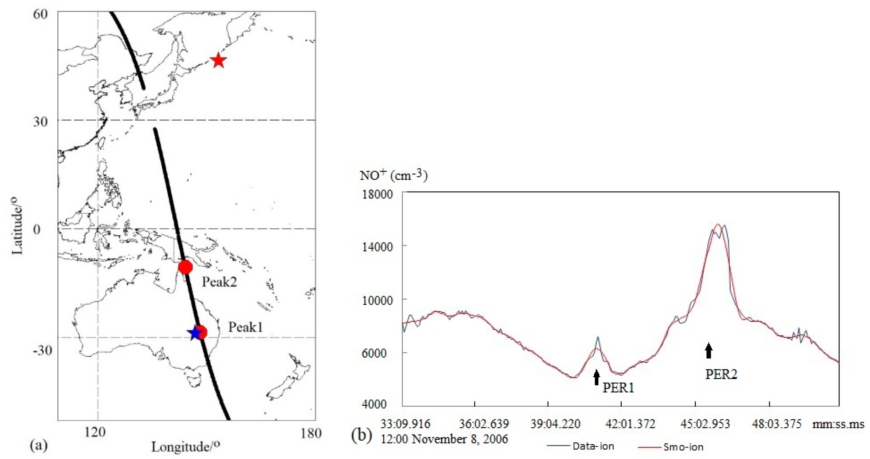
Figure 2.
Distributions of 117,718 ion PERs with respected to the range of Kp index during the DEMETER satellite period considered in this paper.
Figure 2.
Distributions of 117,718 ion PERs with respected to the range of Kp index during the DEMETER satellite period considered in this paper.
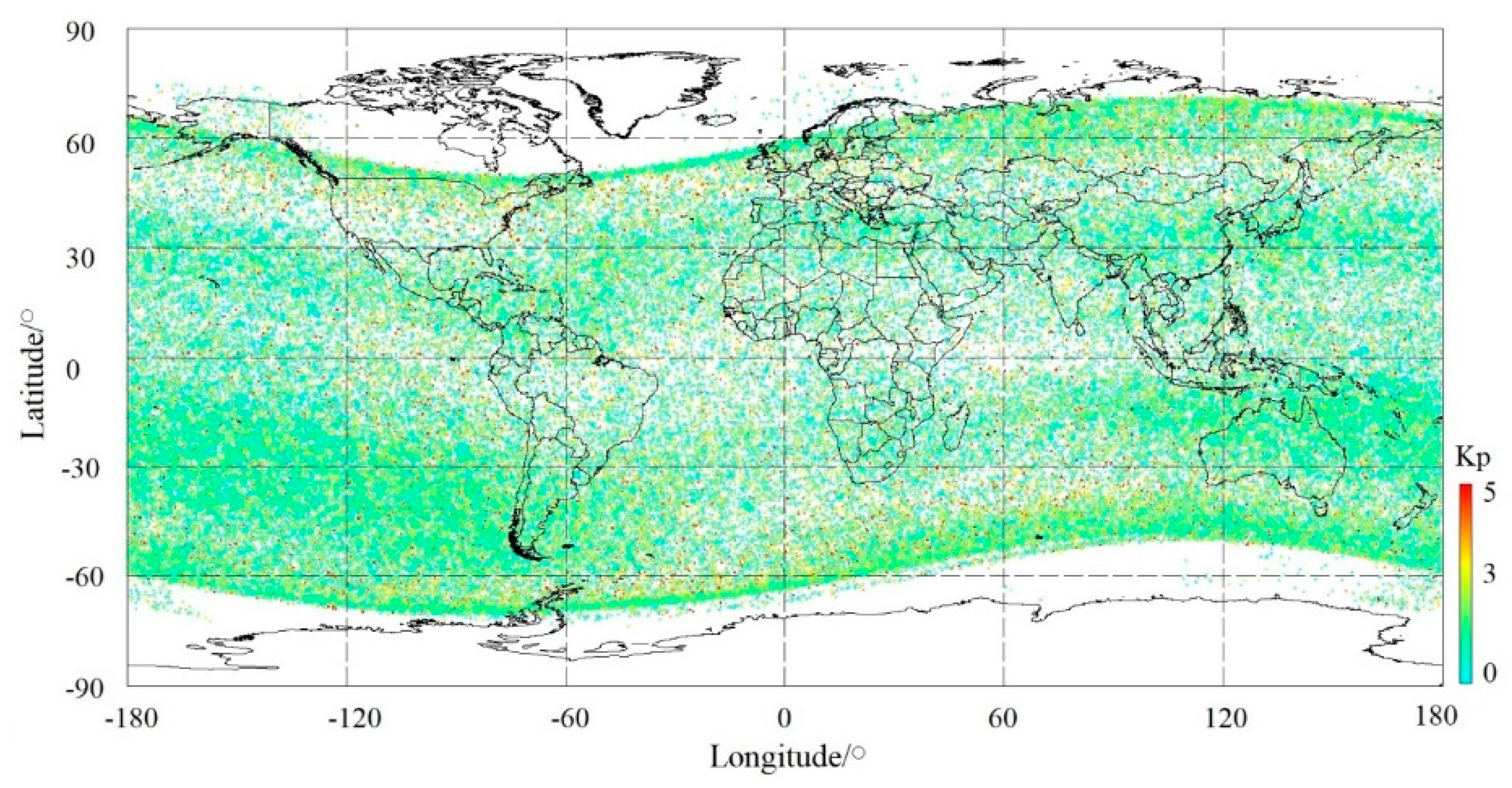
Figure 3.
Polyline of percentages for different groups of perturbations: PERs for Kp > 4 in red line, ones for Kp ≤ 2 in blue line, as a function of (a) an amplitude range (A) and (b) a space size (t) separated from ion density.
Figure 3.
Polyline of percentages for different groups of perturbations: PERs for Kp > 4 in red line, ones for Kp ≤ 2 in blue line, as a function of (a) an amplitude range (A) and (b) a space size (t) separated from ion density.
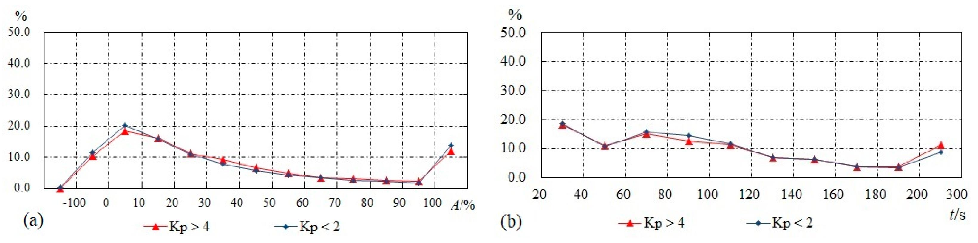
Figure 4.
Polyline of percentages for different groups of perturbations: PERs in nighttime in red line, and ones in daytime in blue line, as a function of (a) an amplitude range (A) and (b) a space size (t) separated from ion density.
Figure 4.
Polyline of percentages for different groups of perturbations: PERs in nighttime in red line, and ones in daytime in blue line, as a function of (a) an amplitude range (A) and (b) a space size (t) separated from ion density.
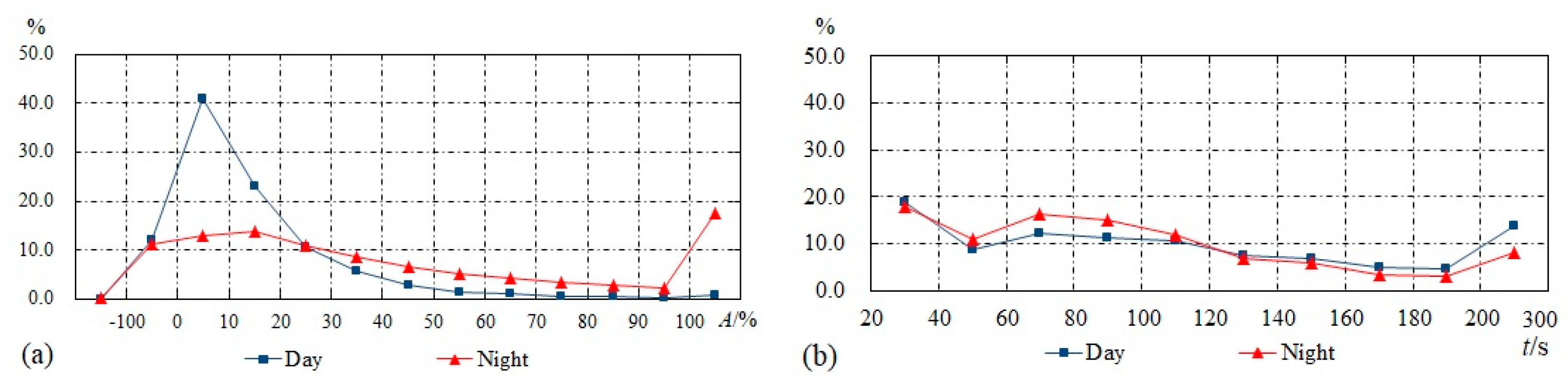
Figure 5.
Distribution of various amplitude ion PERs with respect to different seasons and local time. (a) Daytime in summer, (b) nighttime in summer, (c) daytime in equinox, (d) nighttime in equinox, (e) daytime in winter, and (f) nighttime in winter.
Figure 5.
Distribution of various amplitude ion PERs with respect to different seasons and local time. (a) Daytime in summer, (b) nighttime in summer, (c) daytime in equinox, (d) nighttime in equinox, (e) daytime in winter, and (f) nighttime in winter.
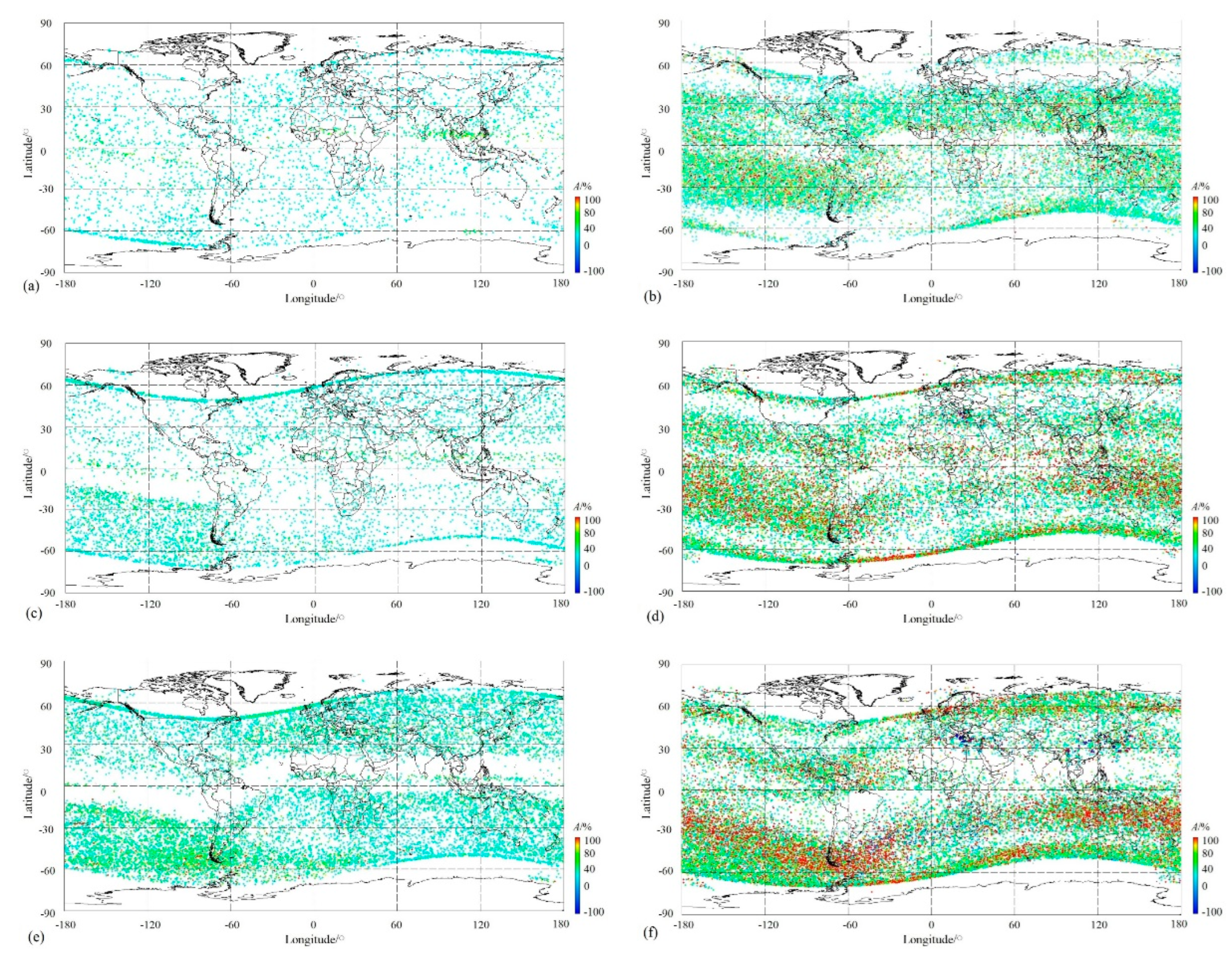
Figure 6.
Distribution of various space size ion PERs with respect to different seasons and local time. (a) Daytime in summer, (b) nighttime in summer, (c) daytime in equinox, (d) nighttime in equinox, (e) daytime in winter, and (f) nighttime in winter.
Figure 6.
Distribution of various space size ion PERs with respect to different seasons and local time. (a) Daytime in summer, (b) nighttime in summer, (c) daytime in equinox, (d) nighttime in equinox, (e) daytime in winter, and (f) nighttime in winter.
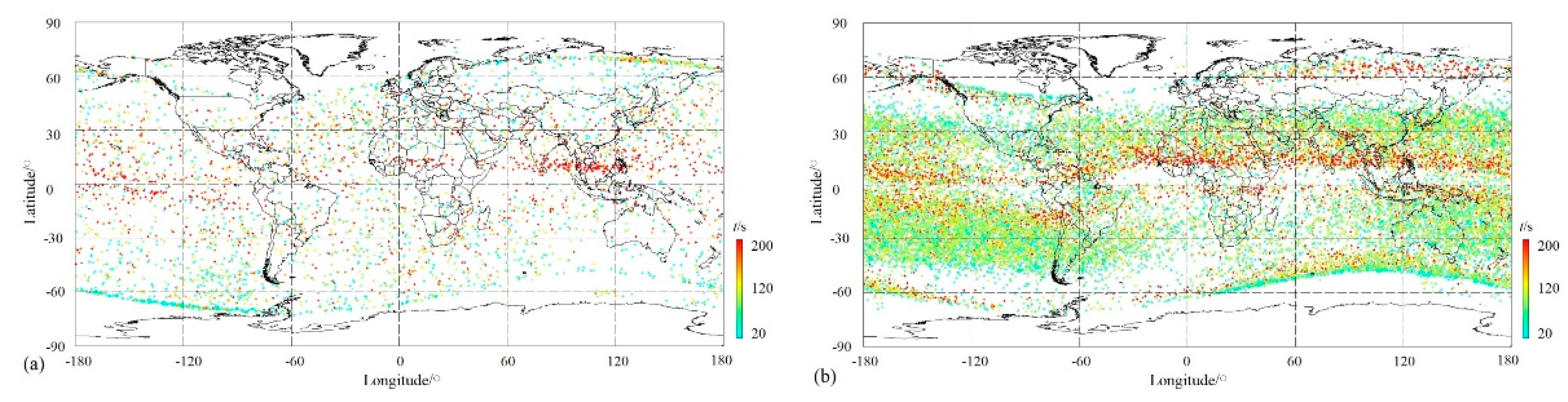
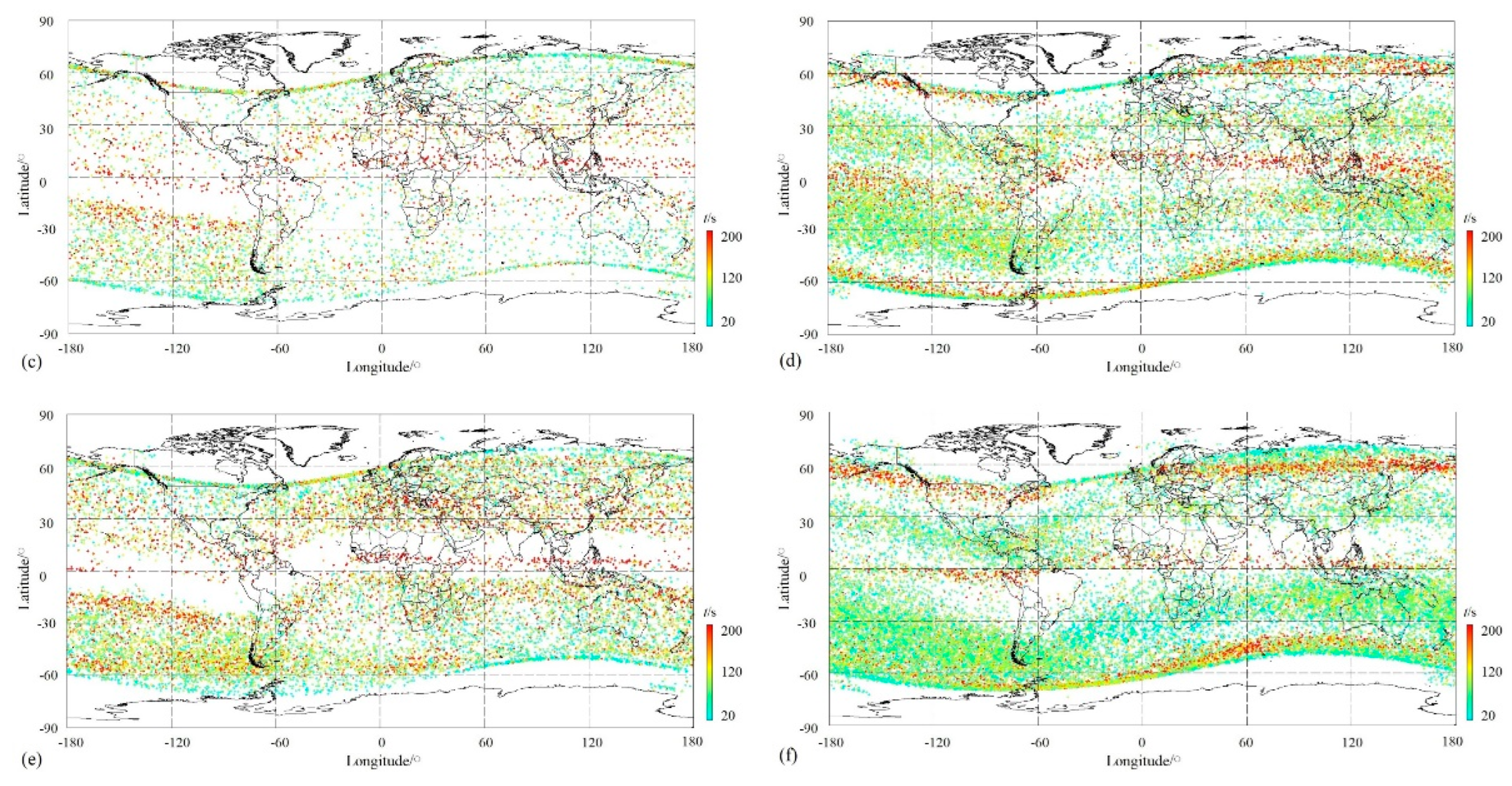
Figure 7.
Distribution of night PERs with respect to various negative amplitude ranges.
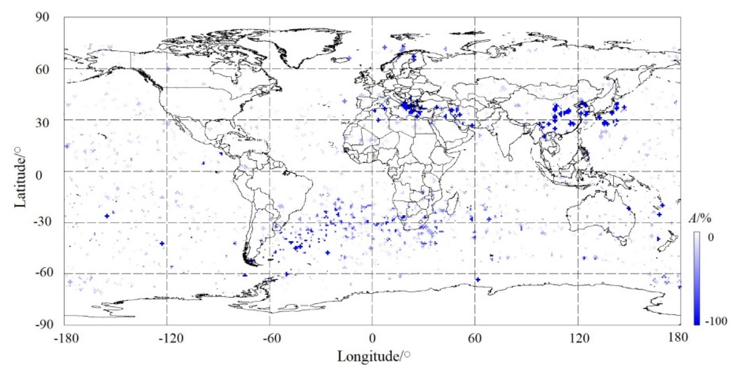

Table 1.
Parameters of two PERs detected by the software along the DEMETER orbit of 12545 at night time.
Table 1.
Parameters of two PERs detected by the software along the DEMETER orbit of 12545 at night time.
| PER1 | PER2 | |
|---|---|---|
| Date (y m d) | 2006 11 8 | 2006 11 8 |
| Time(h m s ms) | 12 41 3 797 | 12 46 0 527 |
| Orbit | 12545_1 | 12545_1 |
| Latitude (°) | -28.5122 | -10.5681 |
| Longitude (°) | 148.210 | 144.081 |
| BkgdIon (cm−3) | 4649.35 | 8378.52 |
| Amplitude(cm−3) | 6738.61 | 14763.6 |
| Trend | Increase | Increase |
| Percent (%) | 44.9 | 76.2 |
| Time_width (m s ms) | 1 37 433 | 4 56 113 |
| Extension (km) | 669 | 2036 |
Table 2.
Number and Percentage of Sub-group of PERs with Different Amplitude (A) for Two Groups of Ion PERs (Kp > 4, and Kp ≤ 2).
Table 2.
Number and Percentage of Sub-group of PERs with Different Amplitude (A) for Two Groups of Ion PERs (Kp > 4, and Kp ≤ 2).
| Kp > 4 | Kp ≤ 2 | |||
|---|---|---|---|---|
| A/% | n | p | n | p |
| ≥100 | 510 | 12.0 | 12014 | 13.8 |
| 90–100 | 100 | 2.3 | 1543 | 1.8 |
| 80–90 | 112 | 2.6 | 1872 | 2.2 |
| 70–80 | 131 | 3.1 | 2292 | 2.6 |
| 60–70 | 151 | 3.5 | 2915 | 3.3 |
| 50–60 | 211 | 4.9 | 3623 | 4.2 |
| 40–50 | 281 | 6.6 | 4850 | 5.6 |
| 30–40 | 388 | 9.1 | 6890 | 7.9 |
| 20–30 | 479 | 11.2 | 9379 | 10.8 |
| 10–20 | 684 | 16.0 | 13881 | 15.9 |
| 0–10 | 776 | 18.3 | 17529 | 20.1 |
| -100–0 | 436 | 10.3 | 10111 | 11.6 |
| <-100 | 4 | 0.1 | 158 | 0.2 |
Table 3.
Number and Percentage of Sub-group of PERs with Different Space Size (t) for Two Groups of Ion PERs (Kp > 4, and Kp ≤ 2).
Table 3.
Number and Percentage of Sub-group of PERs with Different Space Size (t) for Two Groups of Ion PERs (Kp > 4, and Kp ≤ 2).
| Kp > 4 | Kp ≤ 2 | |||
|---|---|---|---|---|
| t/s | n | p | n | p |
| 20–40 | 773 | 18.1 | 16045 | 18.4 |
| 40–60 | 469 | 11.0 | 9121 | 10.5 |
| 60–80 | 646 | 15.2 | 13553 | 15.6 |
| 80–100 | 536 | 12.6 | 12594 | 14.5 |
| 100–120 | 482 | 11.3 | 10200 | 11.7 |
| 120–140 | 287 | 6.7 | 6098 | 7.0 |
| 140–160 | 263 | 6.2 | 5439 | 6.2 |
| 160–180 | 164 | 3.8 | 3255 | 3.7 |
| 180–200 | 158 | 3.7 | 2994 | 3.5 |
| 200–300 | 485 | 11.4 | 7758 | 8.9 |
Table 4.
Number and Percentage of Sub-group of PERs with Different Amplitude (A) for Two Groups of Ion PERs (Daytime and Nighttime).
Table 4.
Number and Percentage of Sub-group of PERs with Different Amplitude (A) for Two Groups of Ion PERs (Daytime and Nighttime).
| Daytime | Nighttime | |||
|---|---|---|---|---|
| A/% | n | p | n | p |
| ≥100 | 249 | 0.9 | 15650 | 17.7 |
| 90–100 | 73 | 0.2 | 2054 | 2.4 |
| 80–90 | 116 | 0.4 | 2486 | 2.8 |
| 70–80 | 148 | 0.6 | 3011 | 3.4 |
| 60–70 | 332 | 1.1 | 3716 | 4.2 |
| 50–60 | 451 | 1.5 | 4562 | 5.2 |
| 40–50 | 844 | 2.9 | 5868 | 6.6 |
| 30–40 | 1699 | 5.8 | 7718 | 8.7 |
| 20–30 | 3104 | 10.6 | 9651 | 10.9 |
| 10–20 | 6712 | 23.0 | 12179 | 13.8 |
| 0–10 | 11983 | 41.0 | 11541 | 13.0 |
| -100–0 | 3515 | 12.0 | 9860 | 11.1 |
| < -100 | 0 | 0.0 | 196 | 0.2 |
Table 5.
Number and Percentage of Sub-group of PERs with Different Space Size (t) for Two Groups of Ion PERs (Daytime and Nighttime).
Table 5.
Number and Percentage of Sub-group of PERs with Different Space Size (t) for Two Groups of Ion PERs (Daytime and Nighttime).
| Daytime | Nighttime | |||
|---|---|---|---|---|
| t/s | n | p | A/% | n |
| 20–40 | 5521 | 18.9 | 15731 | 17.8 |
| 40–60 | 2580 | 8.8 | 9714 | 11.0 |
| 60–80 | 3599 | 12.3 | 14535 | 16.4 |
| 80–100 | 3342 | 11.4 | 13478 | 15.2 |
| 100–120 | 3127 | 10.7 | 10501 | 11.9 |
| 120–140 | 2150 | 7.4 | 6130 | 6.9 |
| 140–160 | 2058 | 7.0 | 5302 | 6.0 |
| 160–180 | 1419 | 4.9 | 3130 | 3.5 |
| 180–200 | 1373 | 4.7 | 2830 | 3.2 |
| 200–300 | 4057 | 13.9 | 7141 | 8.1 |
Disclaimer/Publisher’s Note: The statements, opinions and data contained in all publications are solely those of the individual author(s) and contributor(s) and not of MDPI and/or the editor(s). MDPI and/or the editor(s) disclaim responsibility for any injury to people or property resulting from any ideas, methods, instructions or products referred to in the content. |
© 2023 by the authors. Licensee MDPI, Basel, Switzerland. This article is an open access article distributed under the terms and conditions of the Creative Commons Attribution (CC BY) license (http://creativecommons.org/licenses/by/4.0/).
Copyright: This open access article is published under a Creative Commons CC BY 4.0 license, which permit the free download, distribution, and reuse, provided that the author and preprint are cited in any reuse.


