
Submitted:
05 December 2023
Posted:
07 December 2023
You are already at the latest version
Abstract
This study introduces a multilayer perceptron (MLP) error compensation method for real-time camera orientation estimation, leveraging a single vanishing point and road lane lines within a steady-state framework. The research emphasizes cameras with a roll angle of 0°, predominant in autonomous vehicle contexts. The methodology estimates pitch and yaw angles using a single image and integrates two Kalman filter models with inputs from image points (u, v) and derived angles (pitch, yaw). Performance metrics, including AE, MINE, MAXE, SSE, and STDEV, were utilized, testing the system in both simulator and real-vehicle environments. The outcomes indicate that our method notably enhances the accuracy of camera orientation estimations, consistently outpacing competing techniques across varied scenarios. This method’s potency is evident in its adaptability and precision, holding promise for advanced vehicle systems and real-world applications.
Keywords:
Autonomous vehicles
; camera orientation estimation
; vanishing point
; camera extrinsic parameters
1. Introduction
With the advancements in vision sensor technology, the utilization of vision sensors in advanced driving-assistant systems (ADAS) has become prevalent. The organic incorporation of vision-based sensing technologies such as lane-keeping systems (LKS) and forward collision warnings (FCW) into self-driving scenarios has begun to improve. Most functions are based on vision systems, such as cameras, to obtain the visual context of human perception. Although this pipeline approach of streamlining vision-based inputs to obtain plausible outcomes is common in the ADAS-based industry for accomplishing multiple tasks, such as object detection and segmentation. This is continuously widening the sensing capabilities of self-driving systems [2]. Lane detection is a basic task of an ADAS to identify lane boundaries and extend these to attain LKS and warning systems. Commercial products such as open pilots can be considered successful cases of combining object detection and semantic segmentation into a product with vertical coverage from sensing to control. The simulator also contributes significantly to the regulation and simulation of control systems [3].
Several aspects of the camera, such as its intrinsic and extrinsic parameters (including its position and orientation), are typically used to transform points in the camera coordinate system into a world coordinate system. Conventional camera calibration methods require a calibration target (typically a 2D plane of known size and shape, such as a checkerboard) to determine the intrinsic parameters of the camera. This target is placed in the camera field-of-view (FOV), and a series of images with different angles and distances are acquired. Therefore, geometric transformation techniques can estimate the intrinsic and extrinsic parameters. However, the position and orientation of cameras are still not in practice, particularly when an autonomous vehicle travels through different environments. Therefore, a method for updating camera parameters during real-time online camera calibration is required [4]. The camera parameters can remain updated by updating the intrinsic and extrinsic parameters in real-time. This would ensure a more accurate and reliable autonomous driving system [5].
Camera calibration is also a sub-problem in computer vision. It mainly analyzes known scenes from a sensor from various perspectives and uses these to calibrate the sensor. For example, in the FCW, a practical calculation of the distance between the vehicle and the object ensures a safe distance for the vehicle. This can be affected by the terrain and weather conditions. Single-camera distance estimation assumes that the object and vehicle are on the same plane and projects a 3D object onto a 2D image using calibrated intrinsic and extrinsic parameters of the camera [6]. Because the intrinsic parameters would have been established at the time of production, these do not vary under normal conditions. Meanwhile, the extrinsic parameters represent the relationship between the target coordinate system and the camera coordinate system. The extrinsic parameters are generally updated according to the vehicle’s motion.
There are two methods to calibrate the camera automatically using targetless methods: 1) identify the vanishing point (VP) to estimate the angles (orientations) and 2) determine the area of the object to estimate the yaw and pitch (as described in [7]). Hold et al. used periodic dashed lanes to estimate the initial extrinsic parameters [8]. Paula et al. developed a model to estimate using the VP [9]. Lee et al. estimated the pitch and yaw using a new method in conjunction with VPs [10]. Jang et al. estimated the three angles using three VPs [11]. Guo et al. [12] also developed indoor applications using VPs. These methods accumulate errors in the camera orientation estimation and do not consider error compensation factors.
The contributions of this study are as follows:
- A working pipeline for the multilayer perceptron (MLP)-based adaptive error correction automatic on-the-fly camera orientation estimation algorithm with a single VP from a road lane is proposed (see Figure 1).
- A stable camera on-the-fly orientation estimation variant is proposed. It uses a Kalman filter that can estimate the angular pitch and yaw with respect to the road lane.
- The residual error of using VP to estimate the camera orientation is compensated, and several related compensation modules are compared.
The remainder of the paper is organized as follows. The related work is presented in Section 2. This is followed by the proposed method, including the rotation estimation, system of estimation, and evaluation metrics in Section 3.1. The experimental results are presented in Section 4. The performance of the proposed system and ablation study are discussed in Section 5. Section 6 discusses the limitations of the present study and future work. Section 7 which concludes this study.
2. Related work
Fundamental camera calibration can be categorized into two types: intrinsic (focal length, camera center, and distortions) [13] and extrinsic, which involves mapping rotations and translations from the camera to the world coordinates [14,15] or other sensor coordinates [16,17]. This study focuses on the orientation between the camera and world coordinates. To obtain rotations and translations for online camera calibration, targets such as registered objects [18,19], road marker lanes [20], and objects with apparent appearances [21]are commonly used. However, these methods can not cover the case regarding varying extrinsic parameters. Paula et al. proposed another model to estimate the pitch, yaw, and height for the target-less calibration methods. The generated case was used for extrinsic parameter estimation. Lee et al. proposed an online extrinsic camera calibration method that estimates pitch, yaw, roll angles, and camera height from road surface observations by using a combination of VP estimation and lane width prior. Guo et al. used a more detailed version to estimate the absolute orientation angle. It included the pitch and yaw. They used a method similar to that of Lee et al. and analyzed the failure cases. Although they utilized specific applications considering auto-calibration, their approach had significant errors. These methods cannot prevent projection errors even with an appropriate VP. Jang et al. proposed an online extrinsic calibration approach for estimating camera orientation using motion vectors and line structures in an urban driving environment from three VPs using 3-line RANSAC [22] on a Gaussian sphere. However, the method required more reference lines in the image, and the algorithm was easy to get failed results. To solve this problem, the concept of the reprojection root-mean-squared error [23] for pixels was used. It is a metric used to express the calibration error. This method is a camera-setup-independent error metric used to measure the performance of the calibration algorithm (our model) while omitting extrinsic influences.
For the calibration system, both Lee et al. and Jang et al. proposed stabilization systems using an extended Kalman filter (EKF) to solve the nonlinear system. However, Jang et al. needs more reference lines to get several sets of candidate VPs from 3-line RANSAC on a Gaussian sphere. Therefore, a considerably long time is required to complete the process. The VPs also fail because the selected lines intersect at infinity. Lee et al. has residual error based on the distance from VP and the center point(CP) of the image.
This study proposes an MLP-based error compensation method for automatic on-the-fly camera orientation estimation with a single VP from the road lane and steady-state systems. The method considers the commonly available scenes around a self-driving vehicle. It estimates the pitch and yaw with the correction part using an image.
3. Orientation estimation
It is established that parallel lines do not intersect in the world coordinate system. Thus, we can conclude that the VPs are located at an infinite distance from each other. If we consider the forward direction of a car parallel to the lane lines, we can determine that the lane lines intersect at z = infinity. The road reference frame denotes This point as (X, Y, Z). Here, Z corresponds to the forward axis of the car. It should be noted that the road reference frame is fixed to the vehicle, as shown in Figure 2. Assumptions regarding the alignment of the vehicle with the lane and lane straightness are crucial. This is because the VP, the intersection point of the lane lines in the image, can provide information regarding camera mounting. Specifically, it reveals the orientation of the camera relative to a vehicle. However, if this assumption is not satisfied, the VP would only provide information regarding the orientation of the vehicle in relation to the lane lines and not that regarding the camera orientation.
3.1. Camera Orientation estimation
The camera projection equation with as a point in the image coordinates and as a point in the real-world coordinates is as follows:
where
where K is the camera intrinsic parameter, are extrinsic parameters, the R is the rotation matrix and T is the translation matrix. Because this is an equation in homogeneous coordinates, we can multiply both sides by a scalar value s and absorb this value into Z on the left-hand side of the equation:
The z-axis value of the VP in the world coordinates is infinite. Thus, (4) becomes
The rotation matrix is subject to the pitch, yaw, and roll angles and follows the common case. It is considered to be zero when the camera is mounted on the windshield. The rotation metrics are as follows:
As previously assumed for the roll degree, the rotation matrix represents the yaw and pitch as follows:
As shown in (5), when (6) is substituted into (5), only the third column of information remains. Therefore, the following formula can be used for the two angles:
where is yaw and is pitch radian angle.
Following this function, the reprojection formula can calculate the VPs from the pitch and yaw. In this way, the error () distribution with angle under different camera FOV can be obtained (see Figure 3 and Figure 4). The function that obtains the error is calculated as follows:
where the function f(u,v) is defined as follows:
where , represent the estimated yaw and pitch angle.
3.2. Error compensation of orientation estimation
As mentioned in the previous section, the residual of this model is determined by the camera pose, that is the position of the VP. Since the pitch angle is a sin model, the residual distribution of pitch has a sin relationship with the distance between VP and CP, while yaw is called a tan model. Therefore, the residual distribution of yaw has a tan relationship with the distance between VP and CP. That is, the residual pitch is expressed by From the center of the picture to the edge, a curve approximates a quadratic function, and the residual of yaw appears as an even function about the zero point.
MLP [24]is a conventional method for determining nonlinear coefficients. Considering that the complexity of the nonlinear relationship is moderate and that the correlation is quasi-linear, this study used a shallow network with a rectified linear unit (ReLU) activation function (see Figure 5).
The MLP model is for the VP to estimate the pitch and yaw errors. The two inputs are the distances from the image’s center point to the VP. These are described as and in the image coordinates. The two outputs of the model are the pitch and yaw errors for error compensation.
After the MLP model, the error compensation part would function as follows:
where the MLP model which has trained is:
3.3. Multilayer Perceptron
In this section, we utilize an MLP model as the core component for the error compensation of the angle estimation from the VP. The MLP architecture comprises an input layer, at least one hidden layer, and an output layer. This neural network design aims to generate a specific flow of information between the layers to learn complex representations of the input data.
The MLP network used in this study consists of five linear layers, each with a different number of neurons. The first hidden layer receives two input features and maps these to a 64-dimensional feature space. The subsequent layers increase the feature space to 128 dimensions, gradually decrease it to 64 and 32 dimensions, and produce a 2-dimensional output. The layers are connected through linear transformations (weights and biases) and activation functions such as ReLU. The number of neurons in each layer enables the network to learn higher-level features and abstractions to fit the error distribution.
4. Experimental Result
This section presents the settings and scenarios used in this study. First, to ensure the authenticity of the algorithm verification environment while considering the accuracy and operability of the ground truth(GT) data, the current city simulator was selected (see Table 1). The table outlines the main features and functions of certain highly effective emulators, such as the image resolution, FOV, camera model, camera pose, map generation engine, and minimum hardware requirements. Among these, MORAI has a relatively high accuracy. This map of South Korea was selected as the experimental simulator. An experiment was conducted on IONIQ5, which is used for self-driving research.
4.1. Experimental Environment: Simulator
Table 1 shows the differences. Here, the platforms offer a range of image resolutions. Most of these support a maximum of 1,920 × 1,920 pixels. The FOV for these platforms also varies. A few provide a more comprehensive range of up to and . The camera models utilized by these platforms can be ideal or physical. Specific platforms support both types. The camera poses are indicated by the rotation R and translation T values. These demonstrate the precision in the simulation environment.
From the survey of the simulators, the setting of the MORAI simulator was more suitable for this study. Moreover, it supports the city map of South Korea. The experimental setup of the emulator used in this study is shown in Figure 6. The map was that of Sangam-dong in Seoul, South Korea. The car model was the Kia Niro(EV) 2020 version. The camera model was the default one that supports undistorted image information with adjustable FOV and image resolution. The sensor position and orientation were based on the car coordinates.
To evaluate the stability of the pitch and yaw angle estimation and verify the performance of angle prediction, one angle was fixed, and the other was varied. The scenarios of the experiments are designed as follows in Figure 7:
- Scenario 1: For the algorithm to follow the pitch motion with a variation, it modifies the pitch angle continuously while the yaw angle is fixed to .
- Scenario 2: For the algorithm to follow the yaw motion with a variation, the yaw angle is modified continuously while the pitch angle is fixed to .
- Scenario 3: For the system to converge in certain frames to correct the pitch angle with a variation, the pitch angle is modified by in each frame while the yaw angle is fixed to .
- Scenario 4: For the system to converge in certain frames to correct the yaw angle with a variation, the yaw angle is modified by in each frame while the pitch angle is fixed to .
- Scenario 5: For the system to converge in certain frames to correct the angle with a variation, the pitch and yaw angle is modified by one of them in each frame.
4.2. Experimental Environment: Real Car
To better verify the algorithm in the real world, experiments related to real data were conducted on IONIQ5 vehicles equipped with a GMSL camera (SEKONIX). The camera was located above the windshield. There were two cameras with FOVs of and . In this study, the intrinsic parameters and image undistortion of the camera with were preconfigured fully. Therefore, a camera with a FOV of was used to verify this experiment (see Figure 8). This study used linear lane lines that exist at a short distance from the camera (within about 20m), such as cornerstones or obstacles along the outer edge of the road.
4.3. Result
For each scenario, the table provides the average error (AE), minimum error (MINE), maximum error (MAXE), and standard deviation (STDEV) for all the control algorithms. This enabled the assessment of their performance in terms of accuracy and stability.
To ensure the validity and efficiency of the proposed method, in the system design, a KF is added at the end of the VP and angle estimation process to filter out false VP detections or miscalculations. The performance of Paula et al. consistently exhibits larger error than the method proposed by Lee et al.; therefore, its results are often not visible in the graphs.
Table 2 presents a quantitative analysis of the pitch angle estimation with a fixed yaw angle. As shown in the table, the proposed method outperformed the methods of Paula et al. and Lee et al. regarding the AE, MINE, MAXE, and STDEV. This indicated that the proposed method is more accurate and stable for pitch angle estimation. This is crucial for robotics and computer vision applications. The angle estimation and error curve results are shown in Figure 9.
Table 3 presents a quantitative analysis of the yaw angle estimation with a fixed pitch angle. Compared with the method of Paula et al., the proposed method demonstrated superior performance in the MINE, MAXE, and STDEV. Although the method of Lee et al. performed marginally better in terms of the AE, the proposed method maintained a balanced performance across all the metrics. This demonstrated its effectiveness for yaw angle estimation. The results of the angle estimation and error curves are shown in Figure 10.
Table 4 and Table 5 focuses on the step scenarios with pitch angle estimation under a fixed yaw angle and yaw angle estimation under a fixed pitch angle. The proposed method exhibited advantages regarding specific error metrics such as the MINE and MAXE in both cases. Although the proposed method did not outperform Lee et al. in all the categories, its overall performance remained competitive and stable. This further emphasized the robustness and reliability of the proposed method in various scenarios. The system convergence interval was approximately 30 frames. The angles estimation and error curve result are shown in Figure 11 and Figure 12.
It can be observed from Figure 13 that the proposed method is very close to the lines of the GT and, therefore, has a high accuracy in estimating the pitch angle. The Lee et al. and Paula et al. methods seem to have larger error, especially in some frames, where the errors are pretty significant. In Figure 14, the proposed method again shows very close characteristics to the GT, especially in the error plot; the error of the method is relatively small. However, the yaw angle error of the Lee et al. method is significant in most frames, and although the Paula et al. method seems to be close to GT in some frames, the error is also large in other frames.
Table 6 presents a quantitative analysis of the orientation using three estimation methods to pitch and yaw for real car datasets. The performances of the methods of Paula et al. and Lee et al. and that of the proposed method were compared in terms of the AE, steady-state error (SSE), and STDEV for both pitch and yaw angles.
As observed from the table, the proposed method demonstrates superior performance in terms of the AE and STDEV for both pitch and yaw angles compared with the other two methods. The proposed method achieved the lowest AE for pitch and yaw estimation. This indicated its higher accuracy in orientation estimation for real car datasets. Furthermore, the proposed method displayed the lowest STDEV for yaw estimation and a competitive STDEV for pitch estimation. This illustrated the stability and reliability of the method.
5. Ablation study
This study introduces a compensation module based on the foundational mathematical model proposed by Lee et al. Furthermore, an ablation study was conducted to evaluate the efficacy of various compensation modules. The following methods were analyzed: the original model proposed by Lee et al. (designated as "No process"), Linear Regression (designated as "Linear"), Plane Function Compensation (designated as "Function"), and MLP.
Figure 15 to Figure 18 elucidate the estimation performance of pitch and yaw angles across cameras with different field-of-views (FOVs), specifically 60°, 90°, 120°, and 150°. This exploration covers multiple pivotal aspects:
- Pitch Analysis: The MLP method consistently outperformed other techniques in estimating pitch angles across all FOV ranges. Relative to GT, the estimations from MLP consistently exhibited remarkable accuracy. Conversely, the "No process" method presented substantial deviations from true values.
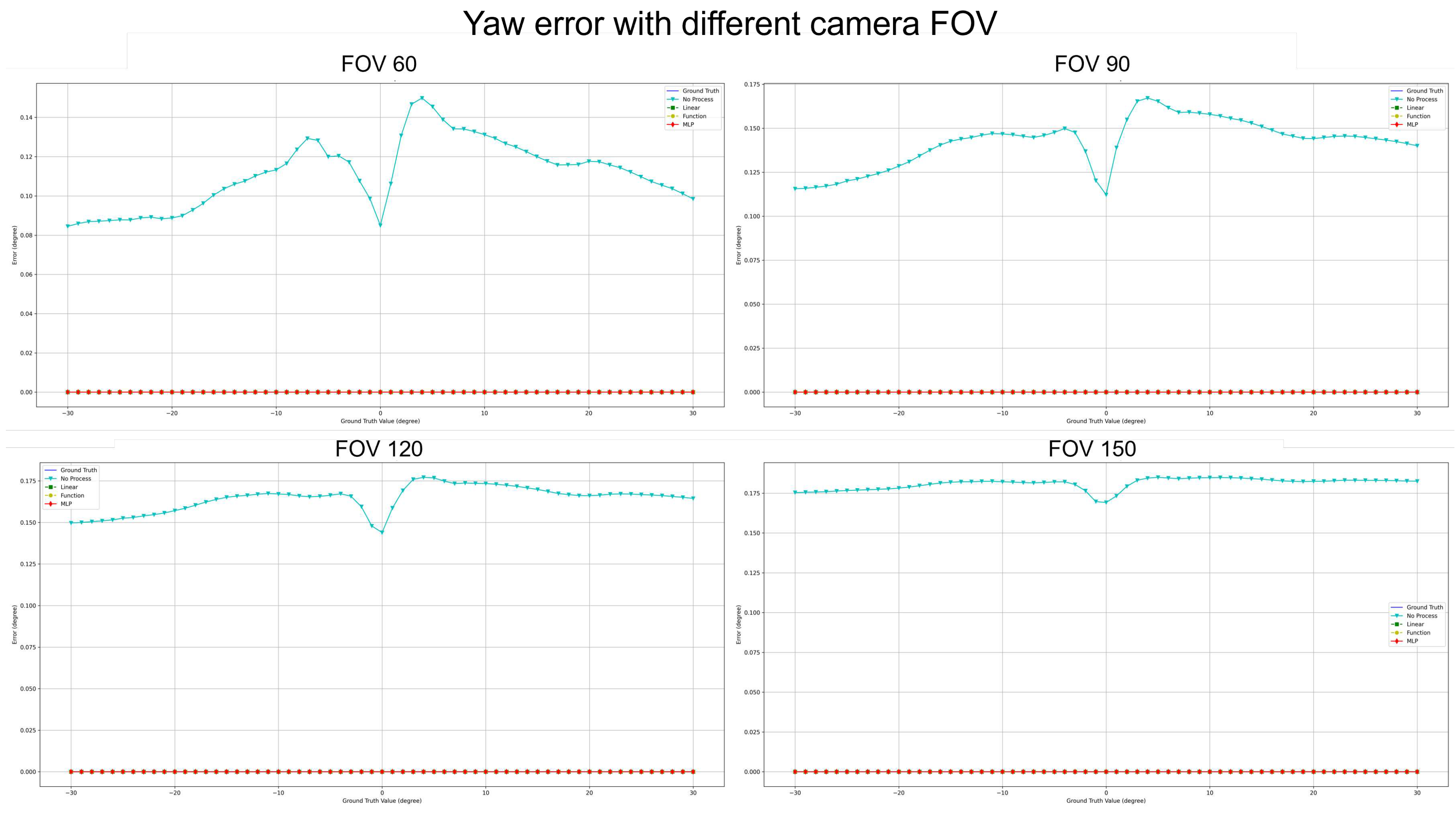
- Yaw Analysis: Several methods achieved commendable precision for yaw estimations across most FOVs. Nonetheless, the "Linear" encountered marginal error increments at specific angles, while the MLP’s accuracy remained relatively invariant.
- FOV Assessment: Across varied FOVs, the MLP method stood out for its pitch and yaw angle estimations accuracy. While the linear and other methods demonstrated efficacy within certain angular ranges, they exhibited noticeable deviations under particular conditions.
Figure 15.
Compensate pitch performance comparison with different camera FOV.
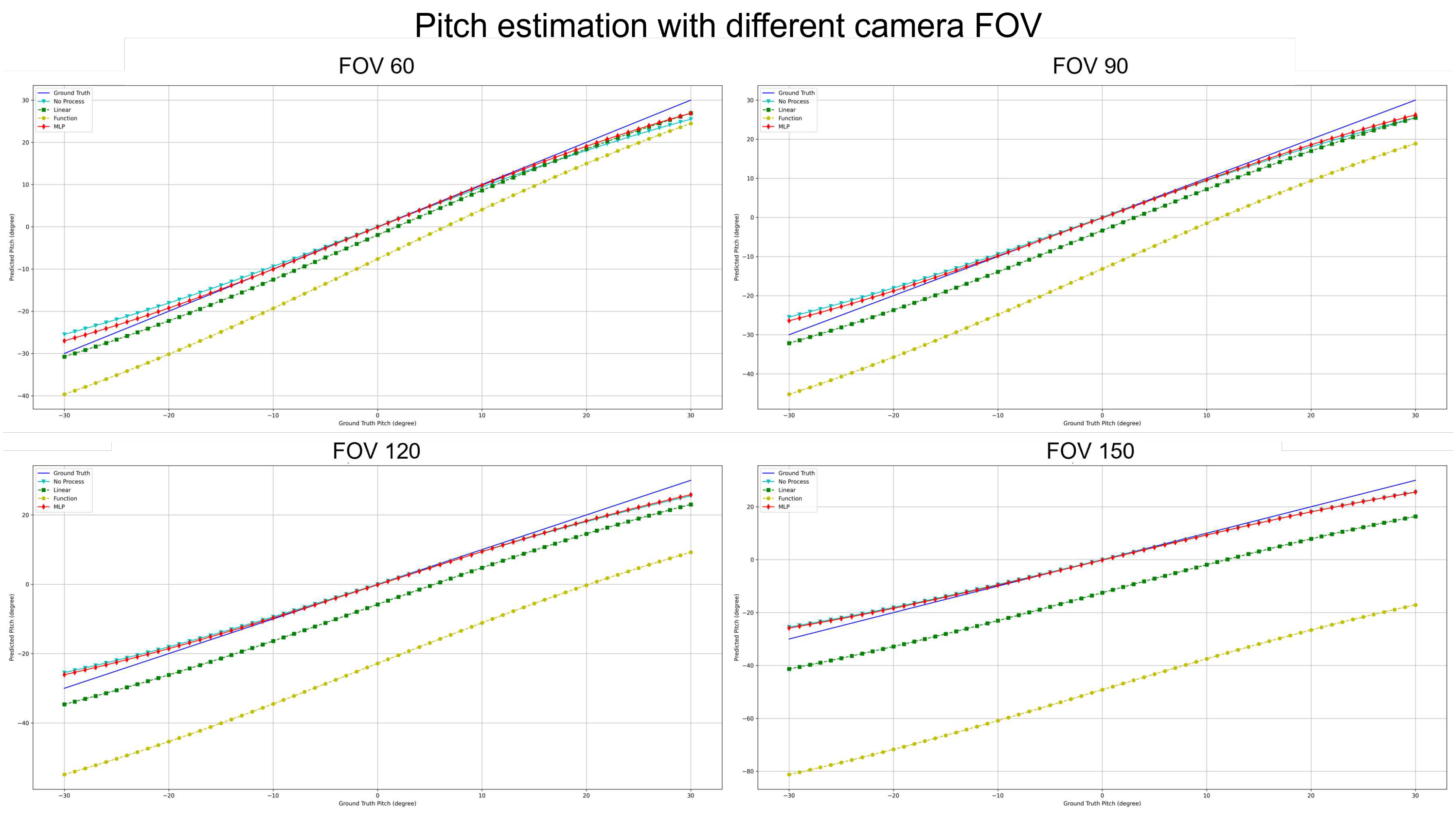
Figure 16.
Compensate yaw performance comparison with different camera FOV.

Table 7 conveys a comprehensive quantitative evaluation of the ablation studies across different FOVs. This table contrasts the performance metrics of the four methodologies on a simulated dataset. Key insights from this analysis include:
- Estimation error for Pitch: Across all FOVs, MLP consistently registered the most minor error. Notably, at a 150° FOV, its performance superiority was markedly evident. The Linear Regression’s error trajectory steeply ascended with FOV increments. Notably, the error magnitude for the "Function" surged most significantly with FOV enlargement.
- Estimation error for Yaw: Astonishingly, both Linear Regression and Function Compensation methods yielded zero error across all FOVs, epitomizing impeccable estimations. Similarly, MLP’s performance mirrored this perfection. In comparison, the "No process" method, while competent, did exhibit a marginal error increase as the FOV expanded.
- Processing Time Assessment: The "Function" consistently achieved the swiftest processing times across all FOVs, signifying optimal resource efficiency. In contrast, the "Linear" generally demanded more prolonged processing intervals. MLP and the "No process" methods displayed commendable consistency in processing durations across all FOVs.
Figure 17.
Compensate pitch error comparison with different camera FOV.
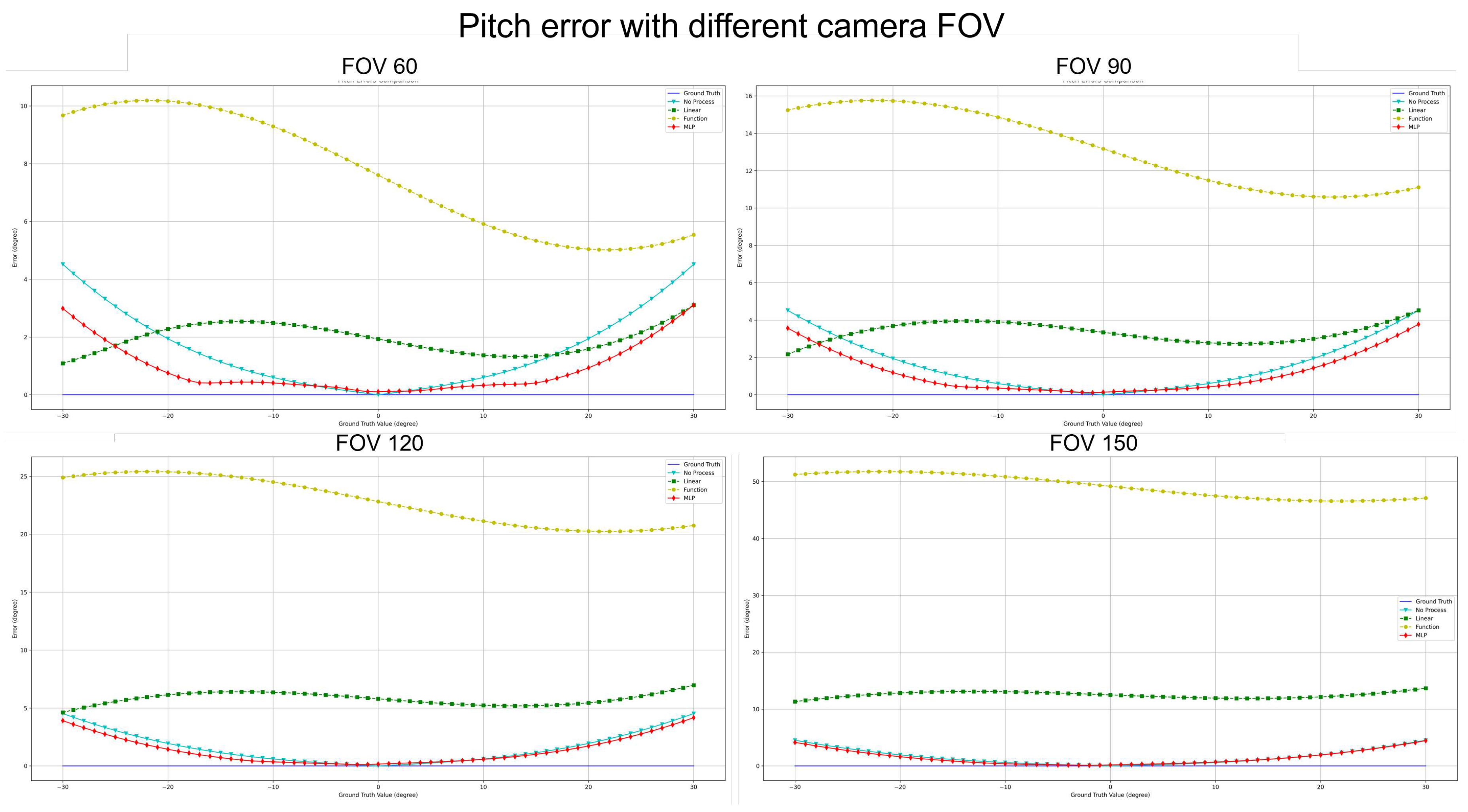
Figure 18.
Compensate yaw error comparison with different camera FOV.
While the MLP methodology showcased exemplary precision in pitch and yaw estimations, its consistency in processing durations substantiated its robustness. "Function," while unparalleled in processing speed, witnessed occasional challenges in estimation accuracy, especially under expanded FOVs. This analysis underscores the intricate balance between speed, resource allocation, and estimation accuracy, suggesting the potential superiority of MLP in wide-ranging practical applications.
6. Discussion
The integration of a compensation module into the foundational mathematical model introduced by Lee et al. marks a significant advancement in enhancing the estimation performance of pitch and yaw angles. This evolution of compensation methods, as evidenced in the ablation study, has profound implications for the accuracy and efficiency of angle estimations. Findings, as represented in Figure 15 to Figure 18, findings underscore the undeniable influence of FOVs on estimation outcomes. The MLP method emerges as a frontrunner, demonstrating consistently superior accuracy across all FOVs.
An intriguing aspect of the study is the Yaw Analysis, which indicates near-perfect estimations by several methods, notably the Linear Regression and Function Compensation. Such impeccable results necessitate further exploration into the factors contributing to yaw’s high accuracy compared to pitch. Such a line of inquiry could be instrumental for future research endeavors. Efficiency analyses shed light on a pivotal trade-off between accuracy and processing time. "Function," while impressively speedy, occasionally falters in accuracy, especially under broader FOVs. The MLP method, while not being the fastest, presents a balanced profile of consistent processing times and commendable accuracy, solidifying its potential in applications where precision is of utmost importance.
The MLP-based technique for camera orientation estimation is promising. However, assumptions like vehicle alignment with the lane and consistent roll angle can lead to inaccuracies. The MLP model may not always capture the intricate relationship between the vanishing point and error distribution. The lack of camera height estimation is a limitation, especially for camera calibration in autonomous vehicles. Future research should focus on improving calibration parameters and refining the error model for various scenarios.
7. Conclusion
This study introduces an MLP-based error compensation method for camera orientation estimation using lane lines and a vanishing point. The aim is to identify an algorithm for Automatic On-the-Fly Camera Orientation Estimation and assess its accuracy. An ablation study compared various compensation modules, including No processed, Linear Regression, Function and MLP. Results showed that the MLP compensation improved the original algorithm’s accuracy, especially in estimating pitch and yaw angles. Future research could expand the calibration approach to include the full rotation matrix and camera elevation. With its potential in autonomous vehicles and driver-assistance systems, the method offers promise for real-time camera orientation tasks.
Author Contributions
Conceptualization, X.L., V.K., and H.K. (Hakil Kim); methodology, X.L., V.K., and H.K. (Hyoungrae Kim); validation, X.L., V.K., and H.K. (Hakil Kim); formal analysis, X.L., V.K., H.K. (Hakil Kim), and H.K. (Hyoungrae Kim); writing—original draft preparation, X.L.; writing—review and editing, V.K., X.L., and H.K. (Hakil Kim); visualization, X.L., H.K. (Hyoungrae Kim), and V.K.; supervision, H.K. (Hakil Kim); project administration, H.K. (Hakil Kim) All authors have read and agreed to the published version of the manuscript.
Funding
This research was supported by the BK21 Four Program funded by the Ministry of Education(MOE, Korea) and National Research Foundation of Korea (NRF).
Data Availability Statement
The data presented in this study are available on request from the corresponding author. The data are not publicly available due to ongoing validations and continuous improvements.
Conflicts of Interest
The authors declare no conflict of interest.
References
- F. Baghaei Naeini, A. M. AlAli, R. Al-Husari, A. Rigi, M. K. Al-Sharman, D. Makris, and Y. Zweiri, “A novel dynamic-vision-based approach for tactile sensing applications,” IEEE Transactions on Instrumentation and Measurement vol. 69, no. 5, pp. 1881-1893, May 2020. [CrossRef]
- A. Gupta and A. Choudhary, “A Framework for Camera-Based Real-Time Lane and Road Surface Marking Detection and Recognition, ” in IEEE Transactions on Intelligent Vehicles,, vol. 3, no. 4, pp. 476-485, December 2018. [CrossRef]
- L. Chen, T. Tang, Z. Cai, Y. Li, P. Wu, H. Li, and Y. Qiao, “Level 2 autonomous driving on a single device: Diving into the devils of openpilot," arXiv preprint arXiv:2206.08176, 2022.
- C. Li and C. Cai, “A Calibration and Real-Time Object Matching Method for Heterogeneous Multi-Camera System," in IEEE Transactions on Instrumentation and Measurement, vol. 72, pp. 1-12, Art no. 5010512, March 2023. [CrossRef]
- Y. Hold-Geoffroy, K. Sunkavalli, J. Eisenmann, M. Fisher, E. Gambaretto, S. Hadap, and J. F. Lalonde, “A perceptual measure for deep single image camera calibration," in Proceedings of the IEEE Conference on Computer Vision and Pattern Recognition, pp. 2354-2363, 2018.
- J. K. Kim, H. R. Kim, J. S. Oh, X. Y. Li, K. J. Jang and H. Kim, “Distance Measurement of Tunnel Facilities for Monocular Camera-based Localization," Journal of Institute of Control, Robotics and Systems, vol. 29, no. 1, pp. 7-14, 2023.
- J. H. Lee and D.-W. Lee, “A Hough-Space-Based Automatic Online Calibration Method for a Side-Rear-View Monitoring System," Sensors, vol. 20, no. 12, p. 3407, June 2020. [CrossRef]
- Z. Wu, W. Fu, R. Xue, and W. Wang, “A Novel Line Space Voting Method for Vanishing-Point Detection of General Road Images," Sensors, vol. 16, no. 7, p. 948, June 2016. [CrossRef]
- M.B.de Paula, C.R. Jung and L.G. da Silveira, “Automatic on-the-fly extrinsic camera calibration of onboard vehicular cameras." Expert Systems with Applications vol. 41, no.4 pp. 1997-2007, 2014.
- J. K. Lee, et al., “Online Extrinsic Camera Calibration for Temporally Consistent IPM Using Lane Boundary Observations with a Lane Width Prior," arXiv preprint arXiv:2008.03722, 2020.
- J. Jang, Y. Jo, M. Shin and J. Paik, “Camera Orientation Estimation Using Motion-Based Vanishing Point Detection for Advanced Driver-Assistance Systems," in IEEE Transactions on Intelligent Transportation Systems, vol. 22, no. 10, pp. 6286-6296, October 2021. [CrossRef]
- K. Guo, H. Ye, J. Gu, and Y. Tian, “A Fast and Simple Method for Absolute Orientation Estimation Using a Single Vanishing Point," Applied Sciences, vol. 12, no. 16, p. 8295, August 2022. [CrossRef]
- D. -Y. Ge, X. -F. Yao, W. -J. Xiang, E. -C. Liu and Y. -Z. Wu, “Calibration on Camera’s Intrinsic Parameters Based on Orthogonal Learning Neural Network and Vanishing Points," in IEEE Sensors Journal, vol. 20, no. 20, pp. 11856-11863, October, 2020. [CrossRef]
- P. Lébraly, C. Deymier, O. Ait-Aider, E. Royer, and M. Dhome, “Flexible extrinsic calibration of non-overlapping cameras using a planar mirror: Application to vision-based robotics," in 2010 IEEE/RSJ International Conference on Intelligent Robots and Systems, pp. 5640-5647, October 2010.
- D. S. Ly, C. Demonceaux, P. Vasseur, and C. Pégard, “Extrinsic calibration of heterogeneous cameras by line images," Machine Vision and Applications, vol. 25, pp. 1601-1614, 2014.
- W. Jansen, D. Laurijssen, W. Daems, and J. Steckel, “Automatic calibration of a six-degrees-of-freedom pose estimation system," IEEE Sensors Journal, vol. 19, no. 19, pp. 8824-8831, October 2019.
- J. Domhof, J. F. P. Kooij and D. M. Gavrila, “A Joint Extrinsic Calibration Tool for Radar, Camera and Lidar," IEEE Transactions on Intelligent Vehicles, vol. 6, no. 3, pp. 571-582, September 2021. [CrossRef]
- L. L. Wang and W. H. Tsai, “Camera calibration by vanishing lines for 3-D computer vision," IEEE Transactions on Pattern Analysis and Machine Intelligence, vol. 13, no. 4, pp. 370-376, April 1991.
- L. Meng, Y. L. Meng, Y. Li, and Q. L. Wang, “A calibration method for mobile omnidirectional vision based on structured light," IEEE Sensors Journal, vol. 21, no. 10, pp. 11451-11460, May 2021.
- M. Bellino, Y. L. M. Bellino, Y. L. de Meneses, S. Kolski, and J. Jacot, “Calibration of an embedded camera for driver-assistant systems," in Proceedings of the IEEE International Conference on Industrial Informatics, Perth, Australia, pp. 354-359, November 2005.
- S. Zhuang, Z. S. Zhuang, Z. Zhao, L. Cao, D. Wang, C. Fu, and K. Du, “A Robust and Fast Method to the Perspective-n-Point Problem for Camera Pose Estimation," IEEE Sensors Journal, vol. 23, pp. 1-1, 2023.
- J. C. Bazin and M. Pollefeys, “3-line RANSAC for orthogonal vanishing point detection," in 2012 IEEE/RSJ International Conference on Intelligent Robots and Systems, Vilamoura, Portugal, pp. 4282-4287, October 2012.
- A. Tabb and K. M. A. Yousef, “Parameterizations for reducing camera reprojection error for robot-world hand-eye calibration," in 2015 IEEE/RSJ International Conference on Intelligent Robots and Systems (IROS), Hamburg, Germany, pp. 3030-3037, September 2015.
- H. Taud and J. F. Mas, “Multilayer perceptron (MLP)," in Geomatic Approaches for Modeling Land Change Scenarios, Cham, Switzerland: Springer, pp. 451-455, 2018.
- G. Rong, B. H. G. Rong, B. H. Shin, H. Tabatabaee, Q. Lu, S. Lemke, M. Možeiko and S. Kim, “Lgsvl simulator: A high fidelity simulator for autonomous driving," in 2020 IEEE 23rd International Conference on Intelligent Transportation Systems (ITSC), Rhodes, Greece, pp. 1-6., September 2020.
- C. J. Hong, and V. R. Aparow, "System configuration of Human-in-the-loop Simulation for Level 3 Autonomous Vehicle using IPG CarMaker," in 2021 IEEE International Conference on Internet of Things and Intelligence Systems (IoTaIS), IEEE, pp. 215-221, November 2021.
- A. Dosovitskiy, G. A. Dosovitskiy, G. Ros, F. Codevilla, A. Lopez, and V. Koltun, “CARLA: An open urban driving simulator," in Conference on Robot Learning (CoRL), Mountain View, California, USA, pp. 1-16, PMLR, October 2017.
- T. V. Samak, C. V. T. V. Samak, C. V. Samak, and M. Xie, "Autodrive simulator: A simulator for scaled autonomous vehicle research and education," in In Proceedings of the 2021 2nd International Conference on Control, Robotics and Intelligent System, pp. 1-5, August 2021.
- M. Rojas, G. M. Rojas, G. Hermosilla, D. Yunge, and G. Farias, "An Easy to Use Deep Reinforcement Learning Library for AI Mobile Robots in Isaac Sim," in Applied Sciences, vol. 24, no. 12(17), pp. 8429, August 2022.
- S. Shah, D. S. Shah, D. Dey, C. Lovett, and A. Kapoor, “AirSim: High-Fidelity Visual and Physical Simulation for Autonomous Vehicles," in Field and Service Robotics: Results of the 11th International Conference, Zürich, Switzerland, pp. 621-635, Springer International Publishing, September 2017.
- C. Park, and S. C. Kee, "Online local path planning on the campus environment for autonomous driving considering road constraints and multiple obstacles," in Applied Sciences, vol. 11, no. 9, pp. 3909, April 2021.
Figure 1.
The framework for automatic on-the-fly camera orientation estimation system.
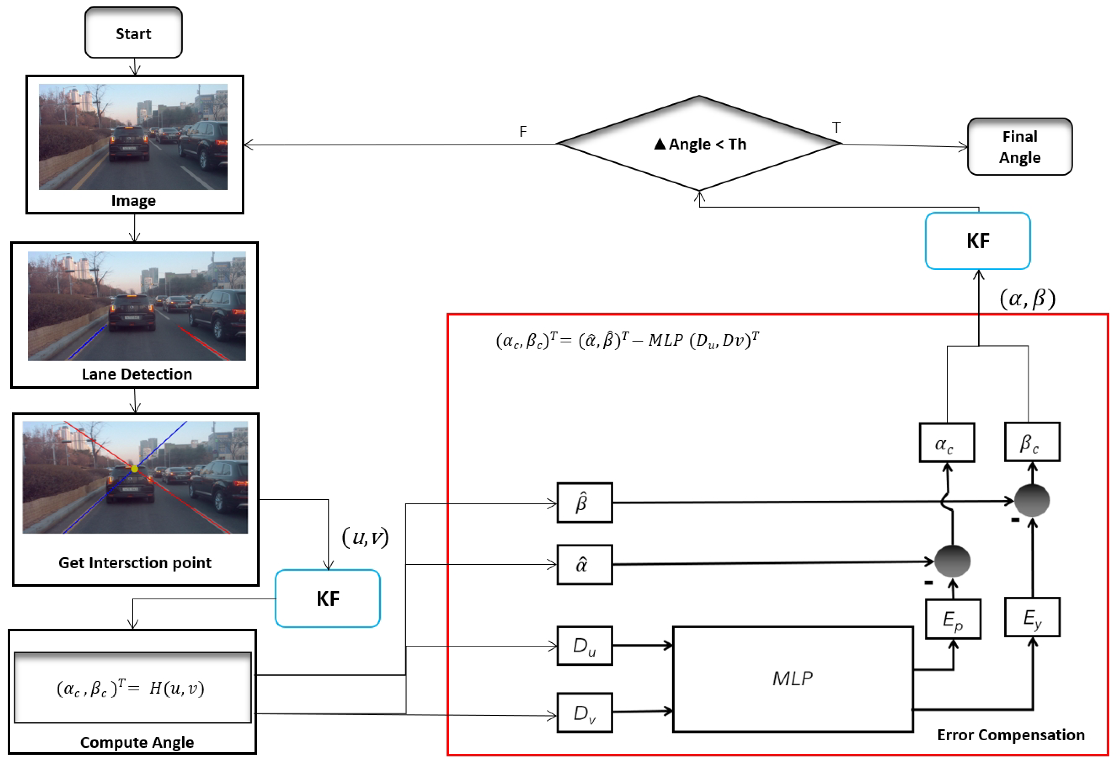
Figure 2.
Camera orientation to road plane and coordinates definition for each coordinate system.
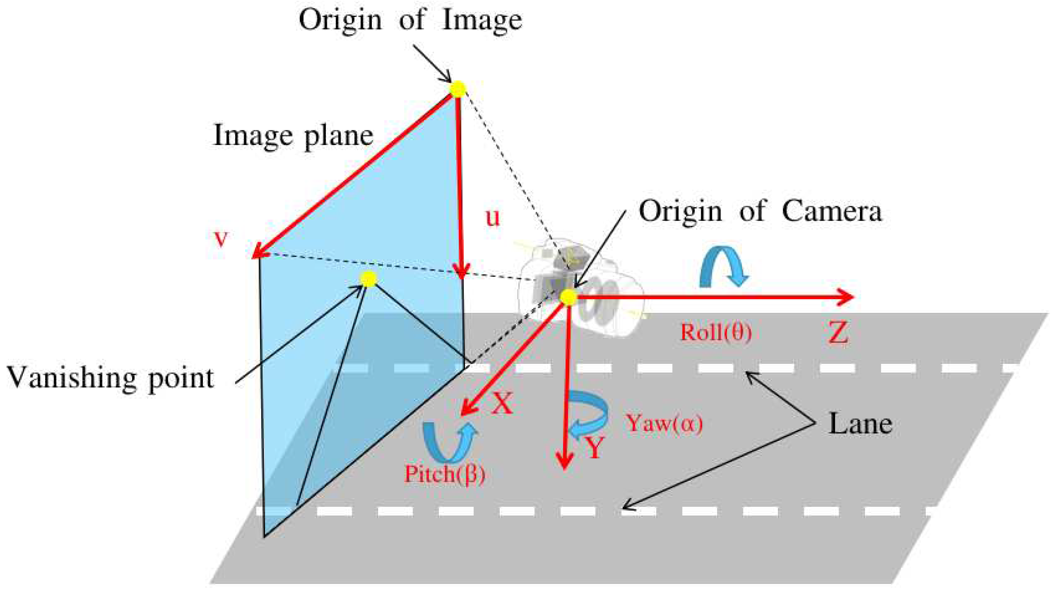
Figure 3.
performance with different camera FOV.
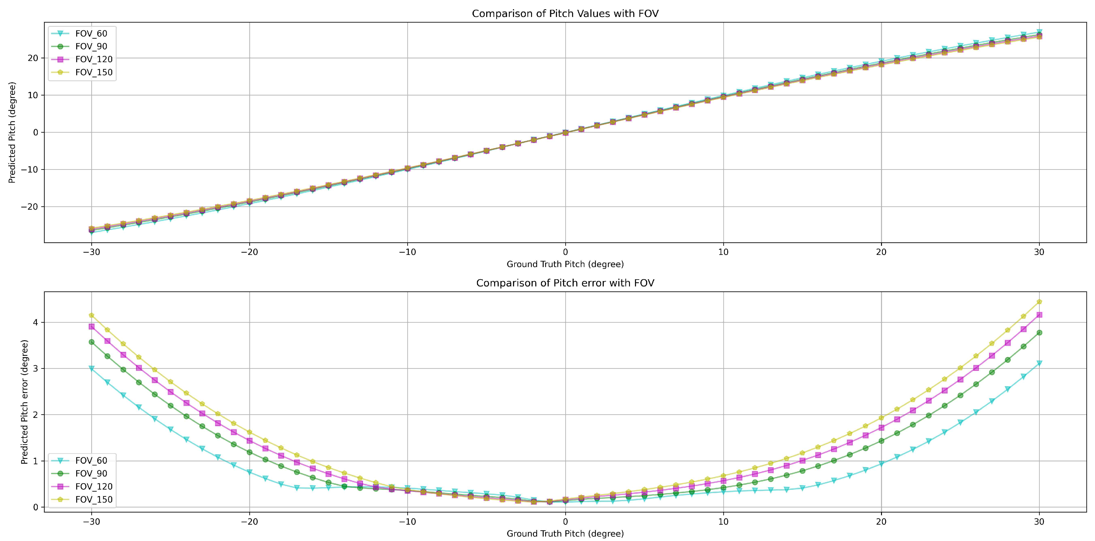
Figure 4.
performance with different camera FOV.
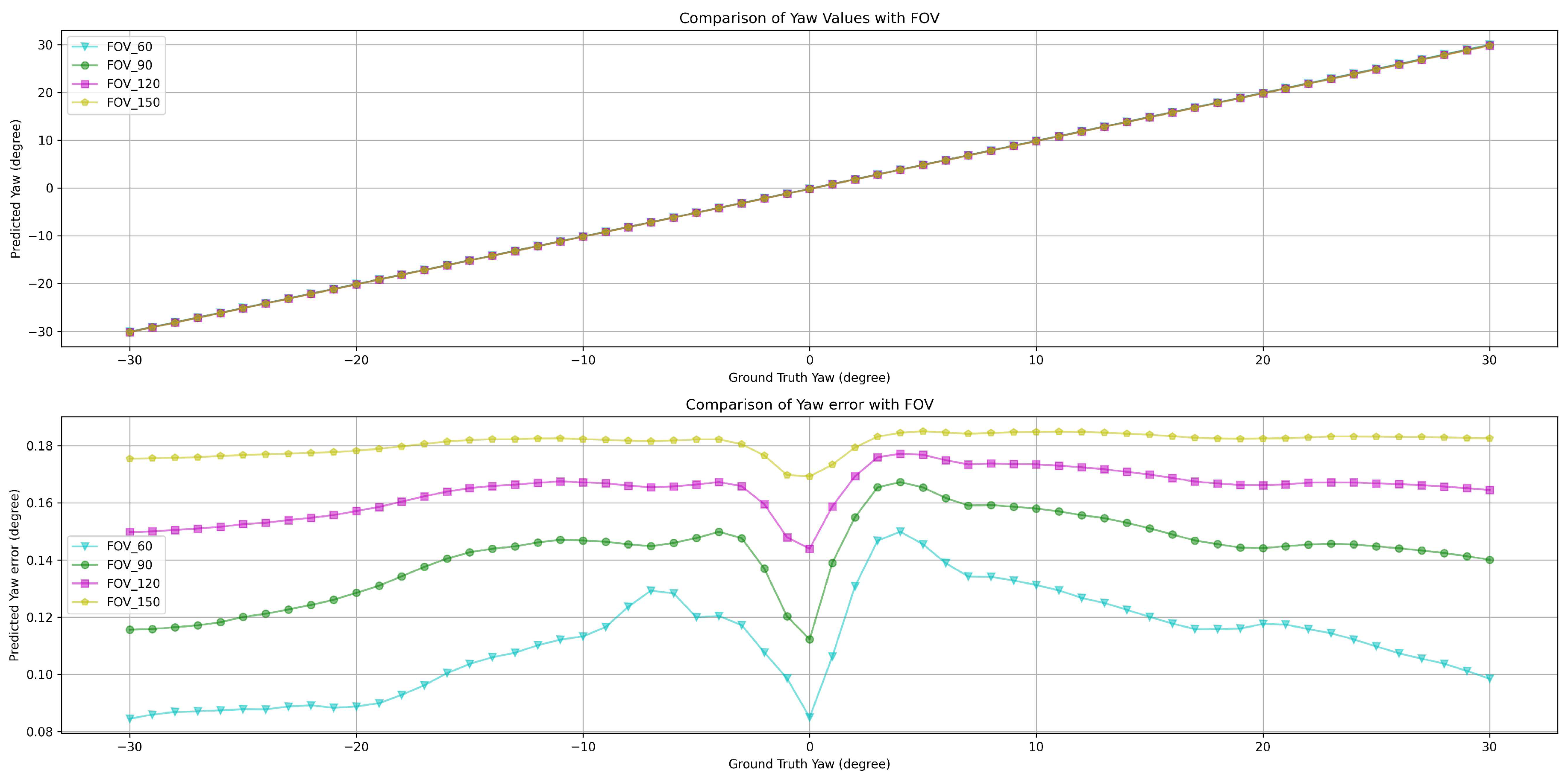
Figure 5.
The MLP model to estimate the error with the VP: The two inputs are the distance from the center point of the image to the VP, whose description as and on the image coordinates. The two outputs are the pitch and yaw error for error compensation, whose description is and on the image coordinates.
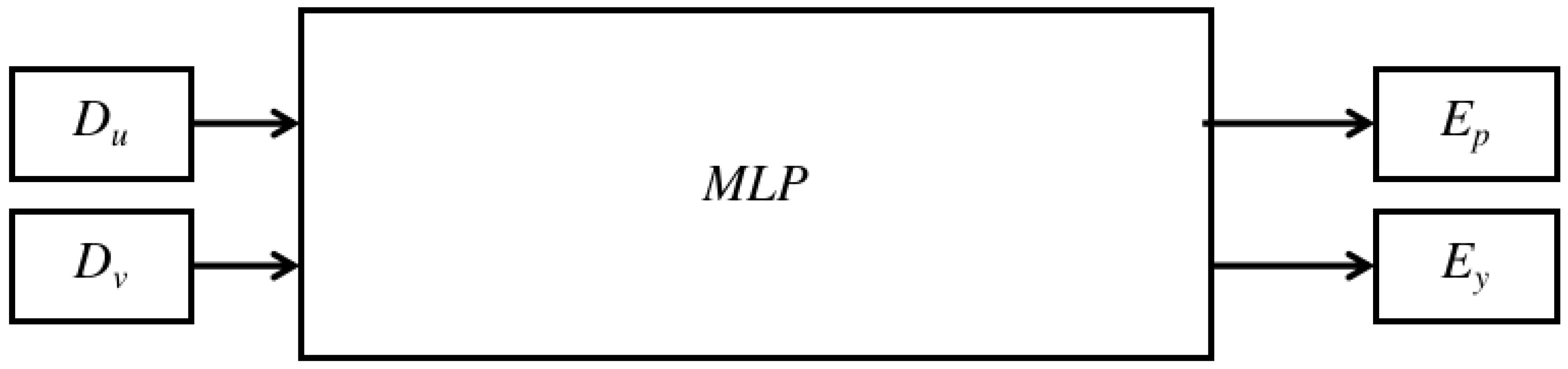
Figure 6.
The settings of MORAI environment and camera.
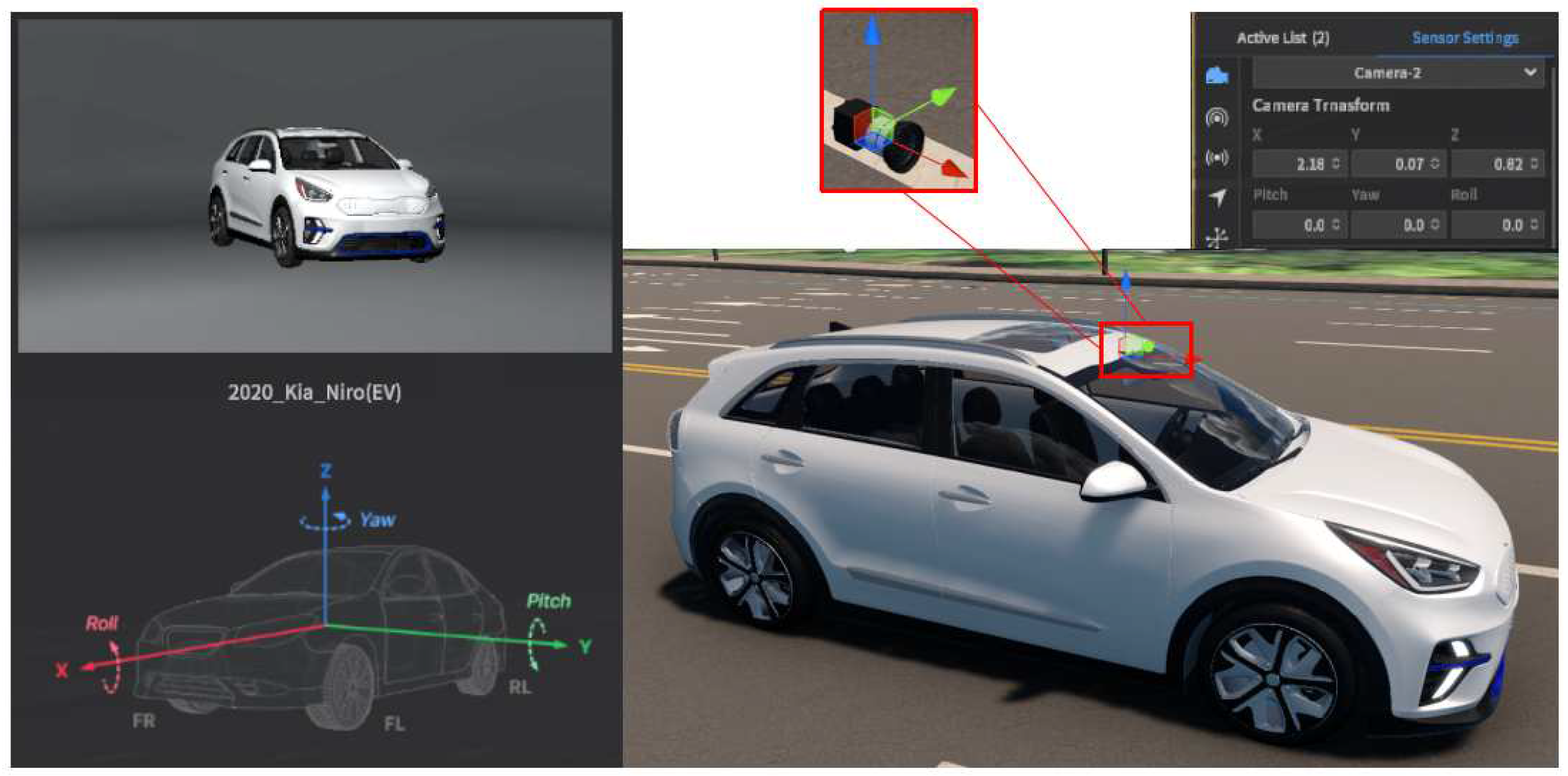
Figure 7.
Scene settings based on transformed angles and changing angles.
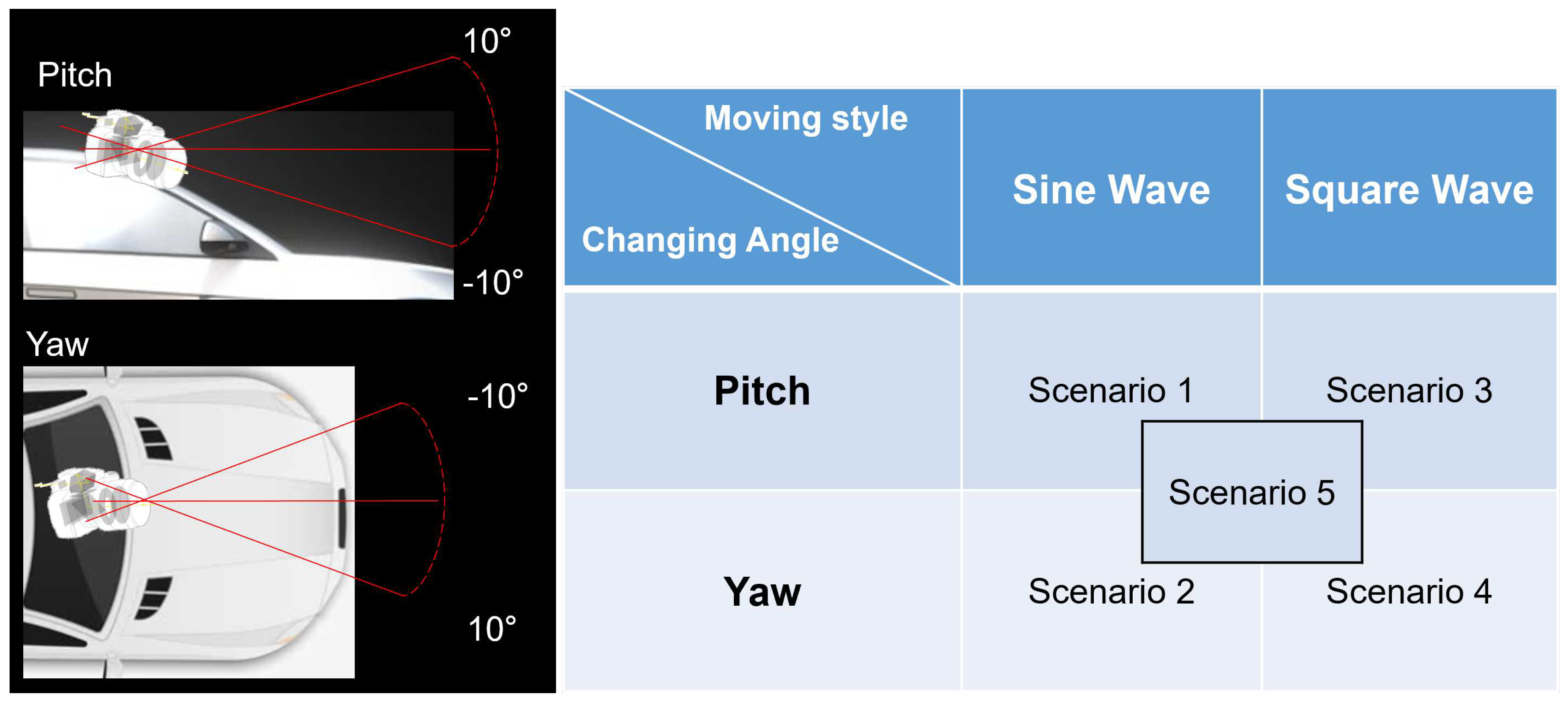
Figure 8.
The settings of real car and camera.
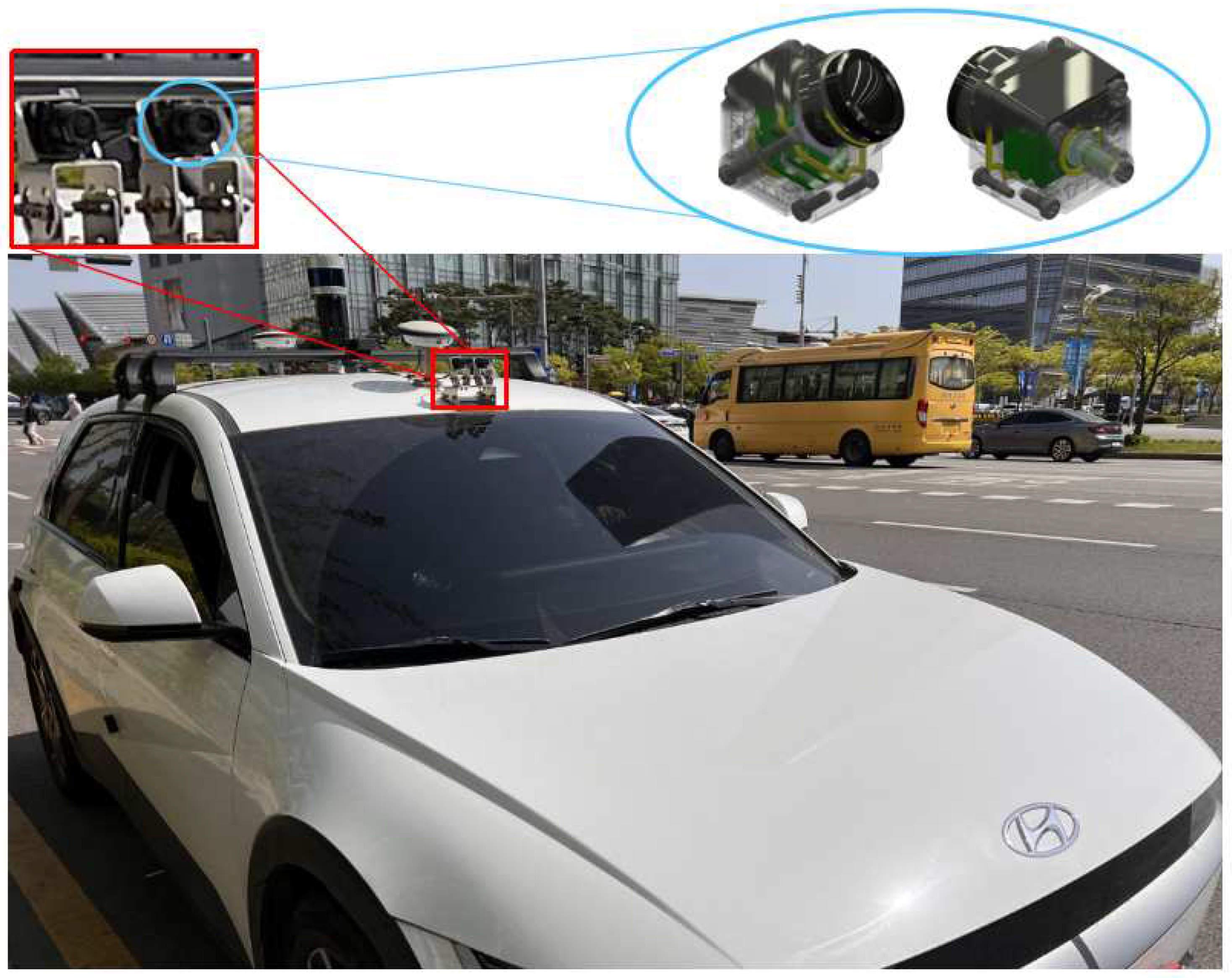
Figure 9.
Performance comparison of three algorithms with Scenario 1.
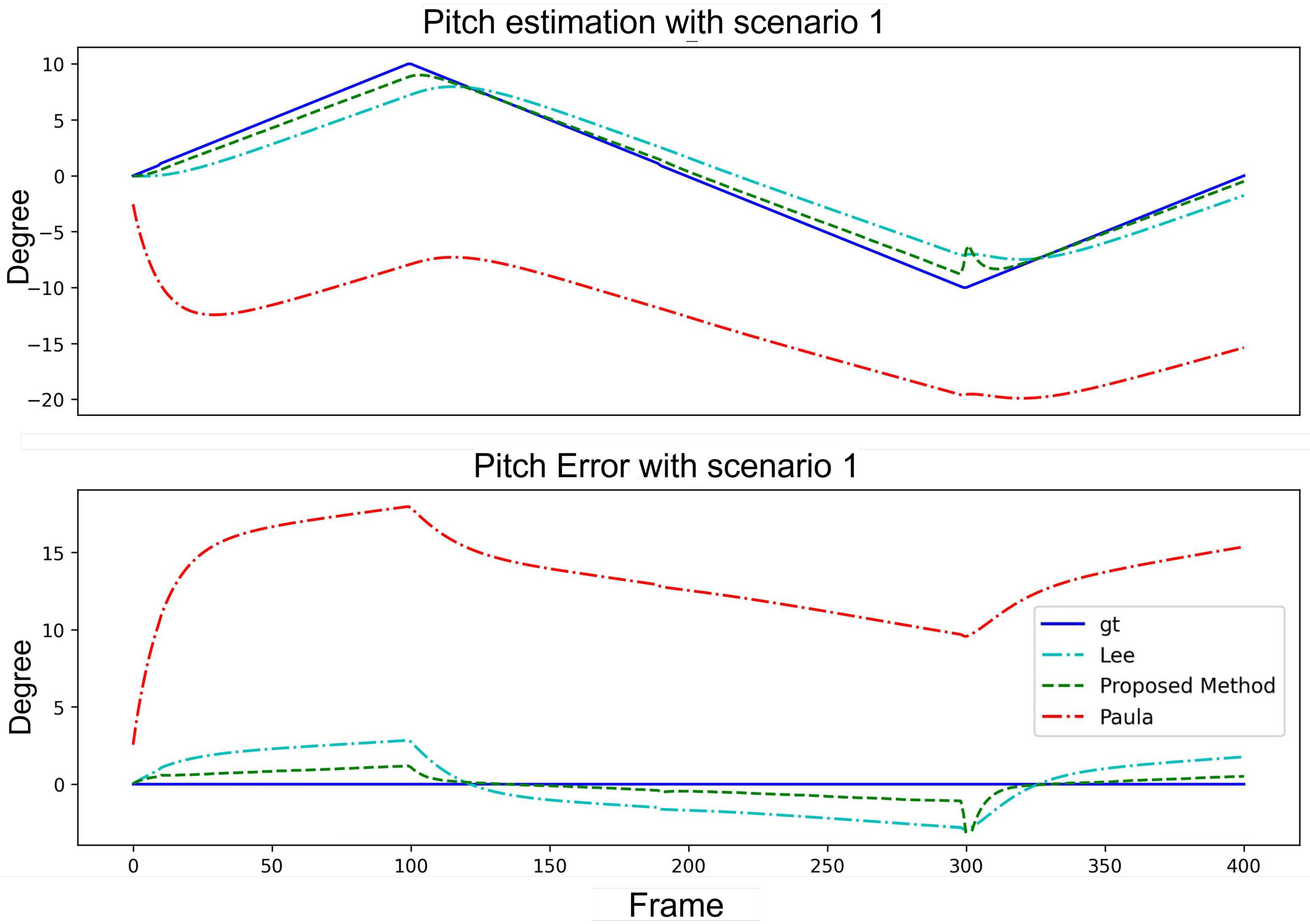
Figure 10.
Performance comparison of three algorithms with Scenario 2.
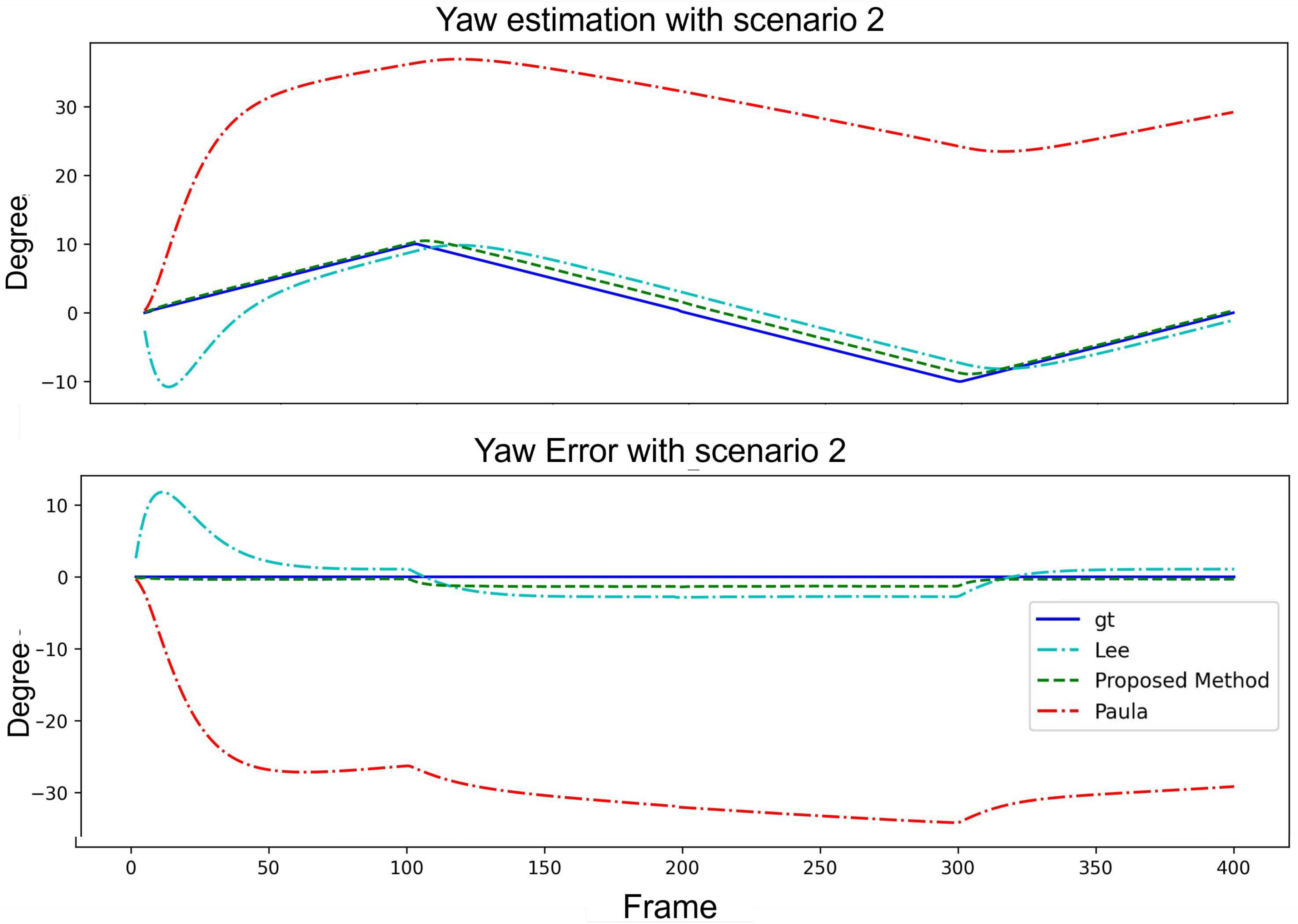
Figure 11.
Performance comparison of three algorithms with Scenario 3.
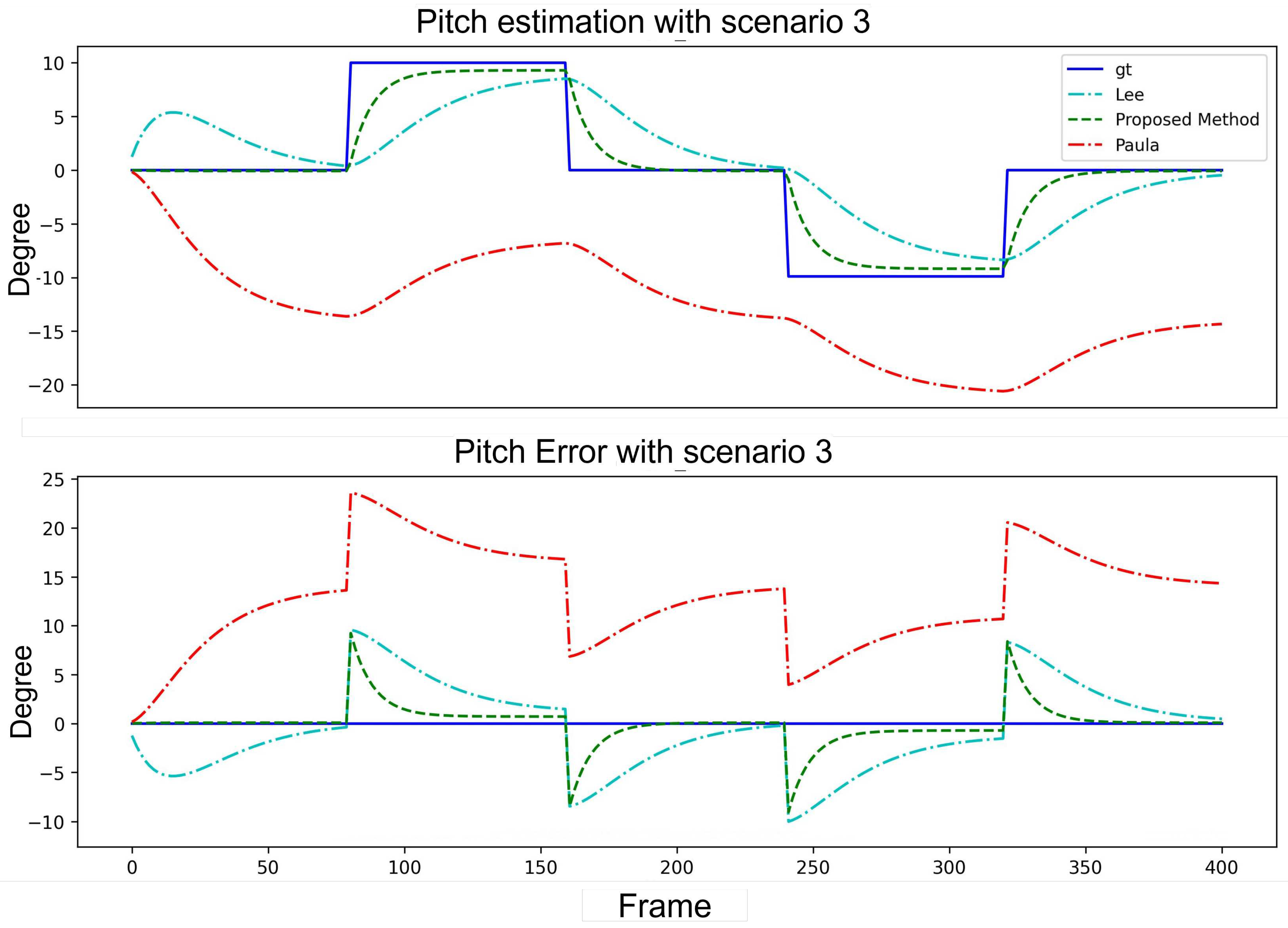
Figure 12.
Performance comparison of three algorithms with Scenario 4.
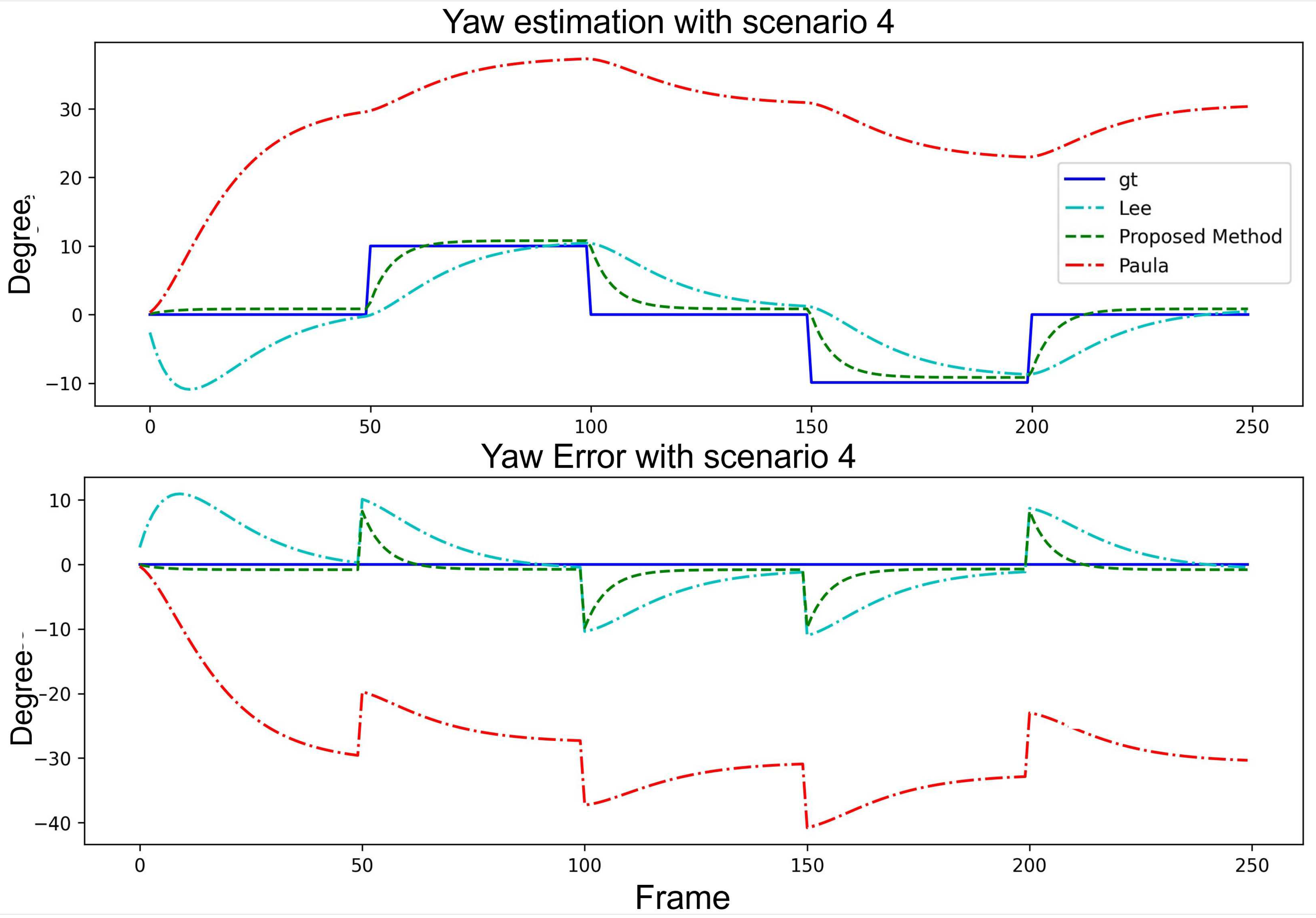
Figure 13.
Pitch performance comparison of three algorithms with Scenario 5.
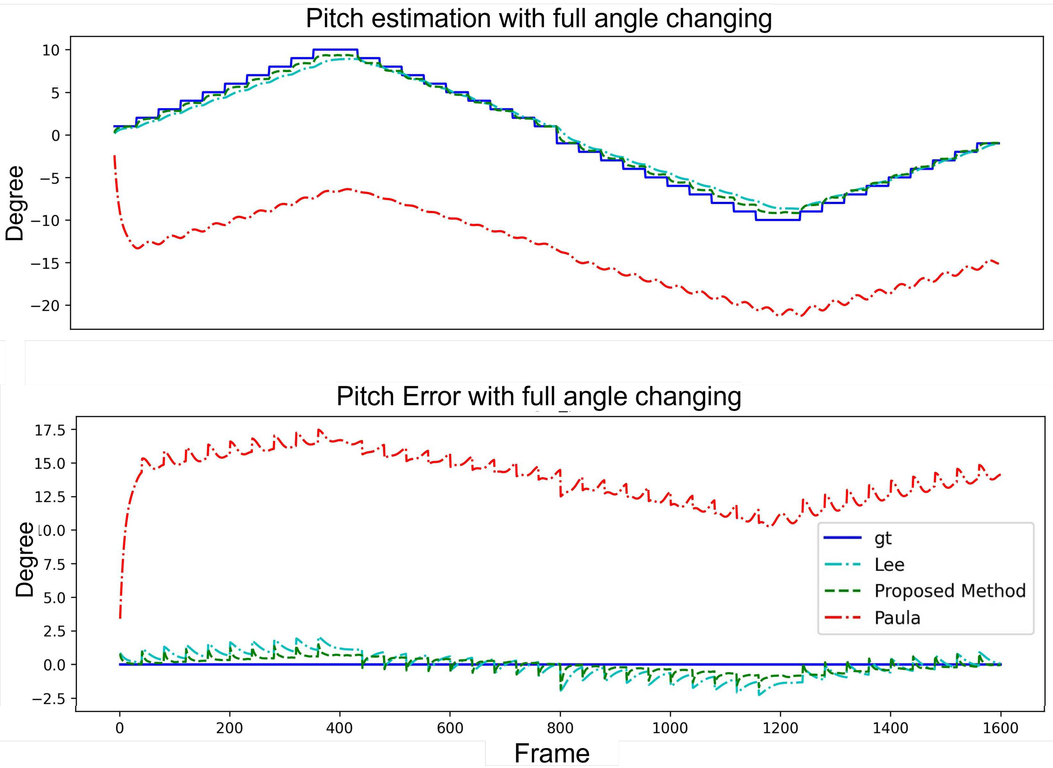
Figure 14.
Yaw performance comparison of three algorithms with Scenario 5.


Table 1.
Comparative Analysis Of Seven Simulators.
| Simulator | Image Resolution | FOV | Camera model | Camera Pose | Map generating | CPU / GPU Minimum Requirements |
|---|---|---|---|---|---|---|
| LGSVL [25] | 0∼1920 * 0∼1080 |
30∼90 | Idea | R(0.1) / T (0.1) | - | 4 GHz Quad core CPU / GTX 1080 8G |
| Carmaker [26] | 0∼1920 * 0∼1920 |
30∼180 | Physical | R(0.1) / T (0.1) | Unity | Ram 4G 1GHz CPU / - |
| CARLA [27] | 0∼1920 * 0∼1920 |
30∼180 | Physical | R(0.1) / T (0.1) | Unity / Unreal | Ram 8G Inter i5 / GTX 970 |
| NVIDIA DRIVE Sim [28] | 0∼1920 * 0∼1920 |
30∼200 | Physical | - | Unity / Unreal | Ram 64G / RTX 3090 |
| Isaac Sim [29] | 0∼1920 * 0∼1920 |
0∼90 | Physical | R(0.001) / T (10e-5) | Unity / Unreal | Ram 32G Inter i7 7th / RTX 2070 8G |
| Air Sim [30] | 0∼1920 * 0∼1920 |
30∼180 | Physical | R(0.1) / T (0.1) | Unity / Unreal | Ram 8G Inter i5 / GTX 970 |
| MORAI [31] | 0∼1920 * 0∼1920 | 30∼179 | Idea/Physical | R(10e-6) / T (10e-6) | Unity | Ram 16G I5 9th / RTX 2060 Super |
Table 2.
Quantitative Analysis Of Pitch Estimation With Scenario 1.
| Paula et al. [9] | Lee et al. [10] | Proposed Method | |
|---|---|---|---|
| AE | 2.551 | 0.020 | 0.015 |
| MINE | 3.865 | 0.130 | 0.120 |
| MAXE | 4.958 | 0.236 | 0.220 |
| STDEV | 2.525 | 1.817 | 1.352 |
Table 3.
Quantitative Analysis Of Yaw Estimation With Scenario 2.
| Paula et al. [9] | Lee et al. [10] | Proposed Method | |
|---|---|---|---|
| AE | -29.109 | -0.105 | -0.566 |
| MINE | 0.307 | 0.017 | 0.002 |
| MAXE | 34.221 | 11.810 | 6.211 |
| STDEV | 5.576 | 3.285 | 1.726 |
Table 4.
Quantitative Analysis Of Pitch Estimation With Scenario 3.
| Paula et al. [9] | Lee et al. [10] | Proposed Method | |
|---|---|---|---|
| AE | -10.392 | 1.465 | 1.731 |
| MINE | -13.210 | -0.088 | -0.057 |
| MAXE | -3.766 | 3.073 | 4.317 |
| STDEV | 5.013 | 5.051 | 5.009 |
Table 5.
Quantitative Analysis Of Yaw Estimation With Scenario 4.
| Paula et al. | Lee et al. | Proposed Method | |
|---|---|---|---|
| AE | -20.334 | 4.523 | 4.804 |
| MINE | 0.307 | 0.673 | 0.112 |
| MAXE | 38.270 | 20.763 | 14.877 |
| STDEV | 13.340 | 9.049 | 6.347 |
Table 6.
Quantitative Analysis Of Orientation Using Three Different Pitch And Yaw Estimation For Real Car Datasets.
Table 6.
Quantitative Analysis Of Orientation Using Three Different Pitch And Yaw Estimation For Real Car Datasets.
| Metric | Paula et al. [9] | Lee et al. [10] | Proposed Method | |||
|---|---|---|---|---|---|---|
| pitch | yaw | pitch | yaw | pitch | yaw | |
| AE | 9.241 | -22.823 | -2.573 | -0.297 | -2.567 | -0.256 |
| SSE | -14.266 | 24.854 | -0.836 | -1.400 | -0.847 | -1.395 |
| STDEV | 2.680 | 2.630 | 0.165 | 0.199 | 0.172 | 0.156 |
Table 7.
Computational Cost Analysis of Each Algorithm.
| FOV | Accuracy | Method | |||
|---|---|---|---|---|---|
| No process | Linear | Function | MLP | ||
| Pitch / degree | 1.572 | 1.944 | 7.606 | 0.881 | |
| 60 | yaw / degree | 0.111 | 0 | 0 | 0 |
| Processing time / ms | 0.025 | 0.098 | 0.003 | 0.063 | |
| FLOPs | 70 | 80 | 120 | 37318 | |
| Pitch / degree | 1.572 | 3.344 | 13.174 | 1.155 | |
| 90 | yaw / degree | 0.142 | 0 | 0 | 0 |
| Processing time / ms | 0.025 | 0.097 | 0.003 | 0.063 | |
| FLOPs | 70 | 80 | 120 | 37318 | |
| Pitch / degree | 1.572 | 5.793 | 22.817 | 1.336 | |
| 120 | yaw / degree | 0.164 | 0 | 0 | 0 |
| Processing time / ms | 0.024 | 0.094 | 0.003 | 0.061 | |
| FLOPs | 70 | 80 | 120 | 37318 | |
| Pitch / degree | 1.572 | 12.482 | 49.164 | 1.473 | |
| 150 | yaw / degree | 0.181 | 0 | 0 | 0 |
| Processing time / ms | 0.024 | 0.096 | 0.003 | 0.062 | |
| FLOPs | 70 | 80 | 120 | 37318 | |
Disclaimer/Publisher’s Note: The statements, opinions and data contained in all publications are solely those of the individual author(s) and contributor(s) and not of MDPI and/or the editor(s). MDPI and/or the editor(s) disclaim responsibility for any injury to people or property resulting from any ideas, methods, instructions or products referred to in the content. |
© 2023 by the authors. Licensee MDPI, Basel, Switzerland. This article is an open access article distributed under the terms and conditions of the Creative Commons Attribution (CC BY) license (http://creativecommons.org/licenses/by/4.0/).
Copyright: This open access article is published under a Creative Commons CC BY 4.0 license, which permit the free download, distribution, and reuse, provided that the author and preprint are cited in any reuse.


