
Submitted:
05 August 2025
Posted:
06 August 2025
You are already at the latest version
Abstract
Single-image based camera auto-calibration holds significant value for improving perception efficiency in traffic surveillance systems. However, existing approaches face dual challenges: scarcity of real-world datasets and poor adaptability to multi-view scenarios. This paper presents a systematic solution framework. First, we constructed a large-scale synthetic dataset containing 36 highway scenarios using the CARLA simulation engine, generating approximately 336,000 virtual frames with precise calibration parameters. The dataset achieves statistical consistency with real-world scenes by incorporating diverse view distributions, complex weather conditions, and varied road geometries. Second, we developed DeepCalib, a deep calibration network that explicitly models perspective projection features through the triplet attention mechanism. This network simultaneously achieves road direction vanishing point localization and camera pose estimation using only a single image. Finally, we adopted a progressive learning paradigm: robust pre-training on synthetic data establishes universal feature representations in the first stage, followed by fine-tuning on real-world datasets in the second stage to enhance practical adaptability. Experimental results indicate that DeepCalib attains an average calibration precision of 89.6%. Compared to conventional multi-stage algorithms, our method achieves a single-frame processing speed of 10 frames per second, showing robust adaptability to dynamic calibration tasks across diverse surveillance views.
Keywords:
highway scenes
; multi-view surveillance
; synthetic dataset
; single-image calibration
; deep learning
1. Introduction
The evolution of camera calibration technology has significantly advanced video-based analysis from 2D planar to 3D spatial domains, providing critical support for 3D vision tasks such as vehicle speed calculation [1,2], spatial coordinate localization [3,4], traffic flow counting [5], and vehicle pose estimation [6,7]. This progress has substantially enhanced the environmental awareness of traffic surveillance systems. While camera calibration has established a mature theoretical framework as a fundamental computer vision technique, automatic acquisition of intrinsic and extrinsic camera parameters remains challenging in traffic surveillance scenarios due to diverse observation perspectives and unpredictable environmental conditions.
Existing automatic calibration methods can be categorized into two technical paradigms: multi-stage approaches and single-image approaches. The former achieves calibration through modularized processes including 2D-3D feature point matching, vanishing point detection, and parameter optimization, while the latter directly derives camera parameters from geometric features in single image. Classic multi-stage approaches based on the Perspective-n-Point (PnP) principle [8,9] establish mapping relationships between 3D spatial points and 2D image points to estimate camera focal length and pose parameters [10,11]. In traffic scenarios, these methods typically rely on static landmarks [12,13] or moving vehicles [14,15,16,17] to construct geometric constraint models. However, their performance is highly dependent on accurate feature point detection, making them susceptible to environmental noise such as illumination variations and shadow interference. Even minor localization errors can lead to significant deviations in calibration results.
As the most distinctive geometric feature in panoramic images, vanishing points reflect the visual convergence characteristics of camera perspective projection, with their image positions determined by both intrinsic and extrinsic camera parameters. In traffic scenes, vanishing points typically arise from two orthogonal directions: the viewpoint direction and the horizontal direction. Consequently, numerous studies have creatively utilized these two vanishing point categories for automatic camera calibration [18,19,20,21,22]. Some approaches further attempt to extract the third vanishing point from vertical objects to satisfy the Manhattan World assumption [23,24]. Nevertheless, these methods encounter challenges in highway scenarios. For instance, geometric constraints from single/dual vanishing points remain limited, necessitating supplementary prior information such as landmark dimensions, lane widths, or camera heights. The Manhattan World assumption only applies to artificial structures rather than most natural environments. Additionally, multi-stage methods involve high computational complexity due to iterative optimization across modules. Particularly for Pan-Tilt-Zoom (PTZ) monitoring cameras, continuous detection of lane markings or vehicle targets to stabilize vanishing point acquisition often prematurely terminates calibration procedures during focal length/pose adjustments.
Therefore, developing efficient and robust fully automatic camera calibration methods holds significant practical value. Based on geometric principles of camera imaging, image perspective features provide critical constraints for solving camera parameters. Compared with traditional algorithms relying on scene priors, deep learning frameworks demonstrate stronger environmental adaptability through data-driven feature extraction mechanisms. Previous studies have demonstrated that convolutional neural networks (CNNs) can localize vanishing points. The work [25] directly regressed vanishing point coordinates from panoramic images. Another category of approaches [26,27] reformulates the vanishing point detection task as a classification problem by discretizing the image space into n×n grids, then using the softmax classifier to predict grid positions containing vanishing points. Similarly, vanishing point representation method [28] based on quadrant partitioning offers new insights for camera parameter estimation. In recent years, deep learning frameworks have extended to end-to-end single-image calibration through supervised learning, directly regressing camera focal lengths and other parameters [29]. The core motivation of these methods stems from utilizing observable visual cues in images, such as horizon features [30,31,32] and scene vector fields [33]. However, in highway scenarios, such visual cues are often weakened due to homogeneous road structures and diverse camera viewpoints, significantly degrading performance of existing methods. More critically, the scarcity of publicly available highway scene datasets remains a persistent challenge, leaving camera calibration research as an unresolved problem.
To address these challenges, this paper proposes an automatic calibration framework for highway surveillance cameras using single-image, featuring three primary contributions. (1) We constructed a large-scale synthetic dataset using the CARLA [34] simulation engine, containing 6 map categories and 36 representative highway segments. Through automated annotation pipelines, we generated 336,249 images with ground-truth calibration parameters. This dataset closely matches real-world highway scenarios in camera perspectives, road geometries, and weather conditions, significantly reducing deep learning models' reliance on real-world data. (2) We developed a deep calibration network (DeepCalib) that synergistically integrates the triplet attention module (TAM) [35]. This architecture enhances semantic representation of perspective projection features, enabling joint estimation of vanishing point coordinates and camera pose parameters from single images while automatically adapting to varying observation viewpoints. (3) We adopted a dual-stage training paradigm combining synthetic pre-training and real-data fine-tuning. Robust feature learning is first performed on synthetic data with augmentation strategies to improve generalization. Subsequent parameter fine-tuning on limited real-world data enables virtual-to-real transfer learning. Experimental results demonstrate this approach significantly enhances model adaptability in complex traffic environments.
The rest of this paper is organized as follows. Section 2 introduces the proposed synthetic dataset. Section 3 details the calibration model, network architecture, and training methodology. Section 4 presents experimental results including comprehensive comparisons with baseline models. Finally, section 5 concludes the study and explores future research directions.
2. Benchmark Dataset
Large-scale annotated datasets play a pivotal role in enhancing the generalization capability of deep learning models for visual perception tasks. However, existing public highway-scene datasets predominantly exhibit single-view limitations and lack complete annotations of camera intrinsic and extrinsic parameters, which hinders their capacity to support the training demands of high-precision visual perception models. While the prior work [3] has released Multi-View Camera Calibration Dataset (MVCCD), the sample sizes remain insufficient to cover the diversity of complex highway scenarios. To address this gap, we constructed a large-scale synthetic dataset using the CARLA [34] traffic simulation platform, employing virtual scene augmentation strategies to explicitly expand data distribution diversity.
We selected 36 arterial roads from 6 virtual city maps as foundational scenarios. Each road randomly deployed three camera groups (left/center/right) to achieve multi-view coverage. A comprehensive weather simulation system was developed using procedural generation for typical meteorological conditions including sunny, rainy, cloudy, foggy, and nighttime scenarios, ensuring deep networks maintain robust performance under diverse weather patterns. The traffic flow simulation module incorporated 33 standardized vehicle models with dynamic adjustment capabilities ranging from sparse to dense traffic conditions, maintaining consistency with real highway vehicle density parameters. To simulate operational boundaries of traffic surveillance cameras, we defined four parameter sampling spaces: field-of-view (FOV) [70°, 120°], pitch angle [-28°, 0°], yaw angle [-40°, 40°], and mounting height [10m, 14.5m]. Random parameter sampling ensures uniform label distribution across image regions, effectively mitigating training biases caused by imbalanced datasets. Figure 1 illustrates representative synthetic scenes that closely resemble real-world highway environments while exhibiting greater diversity in camera viewpoints and road geometries.
The final dataset comprises 336,249 pairs of 1920×1080 resolution RGB images with corresponding annotations. Each annotation file records vanishing point coordinates, pitch angle (), yaw angle (), camera focal length (f), and camera height (h). Data partitioning follows a stratified sampling strategy, allocating samples to training/validation/test sets in 7.5:1.5:1 ratios. Table 1 compares parameter distributions between the real-world dataset (MVCCD_R) and synthetic counterpart (MVCCD_S), demonstrating broader coverage across all dimensions for the proposed dataset.
We systematically demonstrate the parameter distribution characteristics of the constructed dataset by visualizing histograms of vanishing point coordinates, camera focal lengths, and pose parameters. Figure 2 reveals that vanishing point coordinates cover the majority of the image plane. Notably, due to the typical top-down installation of surveillance cameras, vanishing points exhibit a pronounced bias toward the upper image half. This distribution pattern closely aligns with the visual perception of roads receding into the distance in real-world scenarios.
Figure 3 presents statistical histograms of camera parameters in MVCCD_S. The two rotation angles (pitch/yaw) exhibit uniform distributions across their defined angular spaces. The focal lengths demonstrate a broad distribution across 500–1400 pixels, with equivalent focal lengths spanning the operational spectrum from wide-angle to medium-telephoto configurations typical of surveillance systems. Camera height parameters cluster within 10.0–13.5 meters, aligning with empirical deployment standards. The dataset maintains statistical equilibrium across critical parameters, providing an ideal benchmark for validating camera calibration algorithms based on geometric constraints.
3. Methods
3.1. Calibration Model for Traffic Surveillance Cameras
Calibration methods for traffic surveillance cameras have been extensively discussed, with detailed derivations referenced in the work [36]. This section provides a concise overview of the underlying principles. In the standard calibration model, a homogeneous 3D spatial point P = [X,Y,Z,1]T is projected onto the image plane as a 2D point p=[u,v,1]T through the projection matrix .
The general mathematical formulation of M is expressed as M = K[R|T], where K denotes the camera’s intrinsic parameters (including focal length and principal point coordinates), while R and T represent the extrinsic parameters (relative to the world coordinate system), corresponding to the rotation matrix and translation vector, respectively. For traffic surveillance cameras, the calibration parameters can be simplified by establishing a rational world coordinate system (refer to Figure 4). Furthermore, under the assumptions that the camera's principal point coincides with the image center and the roll angle remains zero, the projection matrix M is solely determined by the focal length f, pitch angle , yaw angle , and camera height h.
indicates the ground plane.
As a fundamental characteristic of perspective projection, vanishing points exhibit strong correlations with the camera's focal length, pitch angle, and yaw angle. Their coordinates (u,v) in the image plane can be derived using the following relationships:
where (cx,cy) denotes the coordinates of the principal point. As demonstrated in Equation (2), the focal length f can be derived given the vanishing point coordinates (u,v) , pitch angle , and yaw angle . When combined with the camera height h, these parameters enable the complete construction of the calibration matrix M.
3.2. Single-Image Calibration with DeepCalib
Three-dimensional objects exhibit distinct visual convergence effects after undergoing camera perspective projection transformations. In traffic scenes, geometric deformations and convergence directions of road structures vary significantly across different viewpoints, with these projection patterns universally present in both panoramic images and local objects. This implies that camera parameters can be derived from image projection features. According to this geometric regularity, we developed DeepCalib, a single-image based deep calibration network whose overall framework is illustrated in Figure 5. The DeepCalib architecture comprises three components: a backbone, a deconvolutional module and a multi-task detection head. The backbone network, built on the ConvNeXt [37] architecture, integrates the TAM [35] module for cross-dimensional feature fusion. After feature encoding, three-stage deconvolutional modules perform progressive upsampling, ultimately generating multi-scale feature maps at 1/16, 1/8, and 1/4 resolutions of the original image. The multi-task detection head contains a key point localization branch and a camera pose estimation branch to perform geometric inference from the captured features. Based on the established calibration model, the network outputs are decoded to obtain both intrinsic parameters (focal length) and extrinsic parameters (rotation angles, translation vectors).
3.2.1. Backbone
The backbone network adopts a ConvNeXt architecture to jointly capture global and local visual features. Its hierarchical design incorporates four cascaded ConvNeXt Block modules, constructing multi-scale feature representations through progressive down sampling and channel expansion. For feature extraction, each ConvNeXt Block replaces 3×3 convolutions with 7×7 kernels, maintaining local texture modeling capability while expanding receptive fields to capture long-range spatial dependencies. This design enables joint encoding of global semantic contexts and fine-grained local patterns through enhanced feature hierarchies.
To further enhance cross-dimensional feature interaction, we integrated a TAM module into each ConvNeXt Block. The TAM module comprises three parallel branches targeting channel-height (CH), channel-width (CW), and spatial attention interaction. The CH branch employs dimensional rotation operations to align channel features with height dimensions, while the CW branch performs channel-width dimensional reorganization. Each branch utilizes Z-Pooling for channel dimension reduction followed by sigmoid activation to generate attention weights. This architecture preserves spatial structural information in the original features while enabling adaptive feature recalibration through cross-dimensional attention modulation. The synergistic enhancement of channel-spatial feature representations allows the network to selectively focus on critical geometric structures in complex traffic scenes, significantly improving contextual perception capabilities.
3.2.2. Multi-Task Detection Head
The multi-task detection head adopts a dual-branch architecture comprising a keypoint branch and a camera pose branch, responsible for vanishing point detection and camera pose estimation. The keypoint branch treats the vanishing point along road extension directions as a critical geometric anchor in panoramic imagery. This branch processes 1/4-scale feature maps from the upsampling module, employing two cascaded 1×1 convolutional layers for channel dimension reduction, ultimately generating heatmap at 136×240 resolution. During ground truth generation, a 2D Gaussian kernel was used to construct the vanishing point response region, with peak coordinates corresponding to the true vanishing point location. Sub-pixel localization accuracy is achieved through heatmap peak response decoding, enabling precise geometric anchor localization in complex traffic environments.
For rotation angle estimation, direct regression of continuous angular values is prone to prediction instability. Inspired by the MultiBin [38] architecture, the camera pose estimation branch adopts a classification and central-residual regression strategy. As illustrated in Figure 6, the rotation angle space is discretized into n overlapping bins. The network first predicts a probability distribution over these bins, then performs residual () regression relative to the selected bin's central angle. The final rotation calibration is obtained through summation of the bin center value and predicted residual.
where represents the ground truth, denotes the center angle of the bin and refers to the residual with respect to the center of the bin .
Regarding camera height regression, a hybrid strategy combining global prior and local refinement was employed. We precomputed a mean height () across the entire dataset, with the network only required to predict residual offset () relative to this global prior. This approach significantly reduces parameter search space complexity while maintaining adaptive calibration capability. The absolute camera height for each input image is recomputed by combining the global mean value with the predicted residual offset.
where the height residual is activated using the sigmoid function . . o stands for the specific output of the network.
3.2.3. Multi-Task Loss Function
Based on the network outputs, the loss function of DeepCalib comprises four components: vanishing point classification loss , offset loss , multibin loss , and camera height residual loss . The vanishing point loss is computed using focal loss [39]:
where, (H,W) denotes the heatmap size, and N represents the number of positive samples. The terms and correspond to the ground truth and predicted responses at heatmap position (i,j), respectively. The hyperparameters and , which adjust the loss weights for positive and negative samples, respectively. To compensate for the quantization error due to feature map down sampling, the vanishing point offset loss is calculated as follows:
where P represents the actual vanishing point coordinates, R denotes the down sampling factor. is the true offset, while (the symbol indicates the floor operation).
where is the weighting factor, set to 0.5. The confidence loss is described by the softmax loss for each bin, while aims at eliminating the discrepancy between the predicted and true values within each bin. The calculation formula is as follows:
where m denotes the number of bins covering the true angle, and represents the ground truth angles. For the camera height residual loss , each regression quantity is evaluated using the Smooth L1 loss:
In summary, the total loss function of DeepCalib can be described as follows:
where , , , and are the weighting factors between the sub–loss functions, with .
3.3. Training Details
This section presents a two-stage progressive training paradigm: (1) end-to-end robust feature learning on MVCCD_S without pre-trained weight initialization, followed by (2) task-specific parameter fine-tuning of the multi-task detection head on MVCCD_R. The initial training phase involves the implementation of several data processing procedures.
Preprocessing: During synthetic data generation, viewpoint diversity was simulated through random perturbations of camera parameters. Despite constrained parameter perturbation ranges, certain samples exhibit vanishing points near image boundaries, causing their corresponding heatmap responses to exceed valid perceptual ranges after down sampling. To address this, a data purification step was first implemented to exclude such invalid samples. The retained valid image sequences were then resized to 544×960 pixels as standardized input for supervised training.
Data Augmentation: The training pipeline incorporated three data augmentation techniques: horizontal flipping, spatial translation, and color transformation. Horizontal flipping and random translation were applied with a probability of 0.4. Translation vectors were randomly combined from four directions (up/down/left/right), with two safety mechanisms: (1) a 50-pixel displacement threshold per direction, aborting transformations exceeding this limit, and (2) a maximum translation magnitude of 180 pixels. Void regions generated post-translation are filled using nearest-neighbor interpolation to maintain pixel continuity. During horizontal flipping, simultaneous sign inversion of the yaw angle ensures parameter validity. The color augmentation module includes random jittering of brightness/contrast/saturation and Gaussian noise injection. To prevent over-enhancement, this operation was activated with a probability of 0.2.
Hyperparameter Choice: Vanishing point heatmaps were generated using 2D Gaussian masks with radius r=8, where pixels with mask values ≥ 0.5 were defined as positive samples. For heatmap loss calculation, parameters were configured as and . For angular discretization, pitch angle and yaw angle were partitioned using 3 and 5 overlapping bins, respectively. The specific binning parameters were configured as: 12° width with 4° overlap for pitch angles, and 20° width with 5° overlap for yaw angles. Pre-computed statistical analysis yielded average camera height of 11.83 meters for MVCCD_S and 12.36 meters for MVCCD_R.
Training Strategy: The training process adopted a two-stage paradigm combining pre-training and fine-tuning. During the pre-training phase, comprehensive feature learning was conducted on large-scale synthetic datasets using a batch size of 32 across 20 epochs (157,600 iterations) with an initial learning rate of 2×10⁻³. This stage emphasizes robust representation learning through end-to-end optimization of all network parameters. The subsequent fine-tuning stage focused on task-specific parameter refinement for the multi-task detection head using real-world datasets. This phase employed a reduced batch size of 16 over 10 epochs (6,720 iterations) with an adjusted initial learning rate of 2×10⁻⁵. Both training stages utilized the AdamW [40] optimizer with weight decay regularization and implement dynamic learning rate adjustment: the learning rate was decayed by a factor of 0.1 when validation loss shows no improvement for three consecutive epochs. To accelerate convergence, distributed training was performed across four NVIDIA A800 GPUs using data parallelism.
4. Experiments
To validate the proposed method, we conducted four experiments: (1) ablation studies, (2) transfer learning, (3) camera calibration, and (4) time consumption. All experiments were performed under identical conditions using a unified test set (comprising both MVCCD_S and MVCCD_R datasets), consistent hardware configuration (NVIDIA A800 GPU) and hyperparameter settings to ensure direct comparability of results.
4.1. Ablation Studies
This experiment employed ConvNeXt_base as the baseline architecture and integrates the TAM module to construct an enhanced model. Ablation experiments systematically compared performance differences between baseline and improved models. The study was based on the test set of MVCCD_S, with quantitative analysis performed across four key metrics: vanishing point Euclidean distance, pitch angle absolute error, yaw angle absolute error, and height residual absolute error. Experimental results are presented in Figure 7.
Statistical analysis indicates that the integration of the TAM module significantly enhances the performance of the baseline network. In vanishing point detection, the ConvNeXt_base_TAM model demonstrates clear superiority. Its Euclidean distance errors predominantly fall within the 0-70 pixel range, with an average error of approximately 22 pixels. In contrast, the baseline ConvNeXt_base model exhibits errors spanning 0-150 pixels (average 40 pixels), with extreme cases exceeding 250 pixels. This improvement is attributed to the TAM module's enhanced capacity for capturing spatial features. Angle estimation performance also shows marked enhancements. For pitch angle estimation, the improved model achieves absolute errors concentrated in the 0°-6° range (mean 1.33°), representing a ~25% accuracy improvement compared to the baseline (0°-7°, mean 1.74°). For yaw angle estimation, the TAM module narrows the error range from 0°-12.5° (baseline) to 0°-10°, reducing the average error from 3.94° to 2.45° (~38% reduction). Height residual estimation shows relatively modest but consistent improvements. The improved model achieves errors within 0-2.5 meters (mean 0.89 meters), outperforming the baseline method. Notably, this limited enhancement may be associated with inherent properties of perspective projection features. Specifically, camera height does not directly influence perspective effects, resulting in reduced model sensitivity to height variations.
The ablation experiments indicates that the TAM module effectively strengthens the representation of spatial geometric relationships, with its advantages becoming particularly pronounced when addressing perspective transformations challenges in complex scenes.
4.2. Transfer Learning
This section presents experimental validation of the transfer learning strategy applied to the DeepCalib model. The implementation involved two training paradigms: 1) pre-training from scratch on MVCCD_S followed by fine-tuning on MVCCD_R, and 2) direct training exclusively on MVCCD_R as a baseline comparison.
Figure 8 systematically illustrates the evolution of loss functions under both strategies, including vanishing point heatmap loss, pitch angle estimation loss, yaw angle estimation loss, and camera height residual loss. Global analysis reveals that compared to direct training, the transfer learning model achieves consistently lower loss values across all metrics, with significantly reduced fluctuations in loss curves during training. Although the initial loss for rotation angle training is higher in the transfer learning approach, its curves demonstrate faster convergence. This indicates that pre-training on synthetic data effectively enhances generalization capability.
Figure 9 provides quantitative comparisons on MVCCD_R. For vanishing point detection, the transfer learning strategy constrains Euclidean distance errors within the [0,50] pixel range (mean 16 pixels), significantly outperforming direct training's [0,220] pixel range (mean 29 pixels). In camera extrinsic parameter estimation, absolute errors for pitch and yaw angles are confined to [0°,4°] (mean 1.18°) and [0°,4.2°] (mean 2°), respectively, substantially surpassing direct training results of [0°,13°] (mean 2.90°) and [0°,16°] (mean 3.28°). Camera height residuals are controlled within 1.2 meters (mean 0.42m), improving upon direct training's 0.48m average. All quantitative metrics confirm the superior performance of transfer learning across evaluated dimensions.
To intuitively verify transfer learning efficacy, Figure 10 compares qualitative results of both strategies in real-world vanishing point estimation. The experimental setup comprises four typical road scene groups arranged in side-by-side format: left panels show direct training predictions, while right panels display transfer learning results. Columns sequentially present input images, ground truth heatmaps, and predicted heatmaps. Observations indicate that transfer learning produces consistently stable vanishing point detection across diverse road environments, particularly excelling in complex curved scenarios with heatmap distributions showing greater consistency with ground truth. These qualitative findings align with quantitative results, conclusively demonstrating that the proposed synthetic dataset serves as a valuable complement to real-world data, enabling significant performance improvements in practical applications through transfer learning.
4.3. Camera Calibration
This section comprehensively evaluates DeepCalib's calibration performance in real-world road scenarios through two experiments. As a foundational validation, we first compared DeepCalib with two representative deep learning methods [3,27] that employ classification only and classification combined with central residual strategies, respectively. To assess model adaptability to complex road morphologies, we categorized test datasets into straight and curved road scenarios, using Euclidean distance as the primary evaluation metric. Table 2 systematically presents comparative results of the three methods.
Experimental results demonstrate that DeepCalib significantly reduces vanishing point estimation errors compared to baseline methods. Notably, all algorithms exhibit varying degrees of performance degradation on curved roads. This phenomenon likely arises from weakened linear features in curved roads, which compromises the network's ability to extract perspective transformation features. Despite this, DeepCalib maintains the lowest average Euclidean distance errors (approximately 13 pixels on straight roads and 34 pixels on curved roads), outperforming the second and third-ranked methods by 44/78 pixels and 39/85 pixels, respectively. Error extremes also demonstrate significantly narrower ranges compared to baseline approaches.
Based on the visualized experimental setup (Figure 11), we conducted line segment measurements at three distances (6m, 9m, 15m) along standardized highway lane markings. The reference benchmarks (6m marking intervals and 9m lane spacing) are explicitly annotated through short line segments and their combinations in the image. Critical measurement lines aligned with lane edges converging toward the vanishing point, enabling direct analysis of perspective projection effects. Table 3 presents quantitative results where DeepCalib achieves mean measurements of 6.56m, 9.96m, and 16.88m for the 6m, 9m, and 15m segments, with min-max ranges spanning 3.44-9.18m, 4.77-14.94m, and 9.05-23.43m. Calibration precision reach 90.67%/89.33%/88.80%, outperforming DeepCN [3] by 4.34%/3.44%/2.90%, respectively. Statistical analysis reveals that error fluctuations correlated with vanishing point detection deviations and camera pose inaccuracies under curved road conditions. In contrast, manual calibration achieves centimeter-level precision (≤6cm) with narrower error extremes. Notably, DeepCalib eliminates scene- and object-specific constraints, demonstrating superior adaptability. This enables high calibration accuracy while maintaining operational flexibility, achieving an optimal balance between precision and generality.
Figure 12 visually demonstrates the calibration performance of DeepCalib under various surveillance camera perspectives. Green circles mark the ground truth of vanishing points, while red circles indicate predictions. To qualitatively evaluate camera parameter prediction accuracy, we employed the line segment reprojection visualization strategy: green line segments represent reprojections of the predicted landmark lengths, and red line segments correspond to projections of the single lane width (3.75m). Experimental results indicate that DeepCalib exhibits excellent adaptability to camera perspective variations. Predicted vanishing points show high consistency with ground truth, and the line segment reprojections strictly adhere to perspective transformation principles. Notably, while the errors of vanishing point localization accuracy and projection experience slight increases in curved road scenarios compared to straight sections, overall errors remain within tolerance thresholds. Although current calibration precision still lags behind manual methods, DeepCalib's advantages lie in its computational efficiency and environmental adaptability. These characteristics make it particularly suitable for dynamic calibration of highway surveillance cameras, offering a practical and scalable solution for intelligent transportation systems.
4.4. Time Consumption
To validate the real-time performance of the DeepCalib model in processing 1920×1080 resolution image frames, we systematically recorded temporal consumption results for each processing stage in Figure 13. The experimental protocol decomposed the algorithm workflow into three core modules: vanishing point decoding (VP Decoding), extrinsic parameter decoding (EP Decoding), and camera calibration. Statistical measurements reveals that DeepCalib achieves processing times of 9.72×10⁻² seconds, 1.9×10⁻⁴ seconds, and 1.95×10⁻⁵ seconds for these respective stages. The cumulative processing duration reaches 9.74×10⁻² seconds (approximately 10 FPS), fully satisfying real-time operational requirements. In stark contrast, conventional roadside camera calibration methods typically require tens of seconds to complete calibration procedures due to their multi-stage operational pipelines, which include vehicle trajectory tracking (or lane line detection/vehicle edge detection), vanishing point localization, and parameter optimization. Notably, vehicle trajectory tracking demands prolonged accumulation of traffic flow to stabilize vanishing point coordinate extraction. DeepCalib circumvents these limitations entirely, requiring only a single highway image frame to accomplish rapid camera calibration within minimal temporal constraints. This remarkable efficiency gain stems from the model's end-to-end architecture design, enabling a substantial performance advantage over traditional methods in processing efficacy.
5. Conclusions
This study addresses the bottlenecks in existing automatic calibration methods for traffic surveillance cameras, focusing on resolving two critical challenges: the scarcity of labeled datasets and poor adaptability to multi-view scenes. We first constructed a large-scale synthetic dataset through simulation of highway scenarios, establishing an effective data augmentation framework. Subsequently, we proposed DeepCalib, a deep calibration network that integrates the triplet attention mechanism to enhance the representational capacity of geometric visual cues, enabling simultaneous vanishing point detection and camera extrinsic parameter estimation. The method operates on single highway images without requiring continuous object detection, significantly improving calibration efficiency. To enhance real-world robustness, we adopted the pre-training and fine-tuning strategies. Experimental results on proposed benchmark dataset demonstrate that DeepCalib adapts to diverse highway surveillance camera views. Its simple yet efficient architecture shows practical value for real-world applications. While achieving promising performance, calibration accuracy for curved road scenarios requires further improvement. Future work will focus on expanding the real-world highway dataset to better meet deep learning requirements. Additionally, we aim to strengthen utilization of local visual cues (e.g., vehicles) for more comprehensive perspective feature representation. Addressing these challenges will hold significant potential to advance automatic traffic surveillance camera calibration technology.
Author Contributions
Conceptualization, W.Z. and W.J.; methodology, W.Z.; software, W.Z.; validation, W.Z., W.L.; formal analysis, W.Z.; investigation, W.Z. and W.J.; resources, W.Z.; data curation, W.J. and W.L.; writing---original draft preparation, W.Z.; writing---review and editing, W.Z.; visualization, W.Z. and W.L.; supervision, W.J.; project administration, W.J.; funding acquisition, W.Z. All authors have read and agreed to the published version of the manuscript.
Funding
This research was funded by the Scientific Research Projects of the Education Department of Shaanxi Province (23JK0371), the Natural Science Basic Research Projects of Shaanxi Province (2024JC-YBQN-0725), and the Talent Launch Projects of Shaanxi University of Technology (SLGRCQD2318).
Data Availability Statement
The dataset used in this research has been published in https://github.com/WenTao10/Multi-View-Camera-Calibration-Dataset.
Acknowledgments
In the preparation of this manuscript, we used the CARLA simulation platform for dataset production and extend our appreciation to them. We have reviewed and edited the output and take full responsibility for the content of this publication.
Conflicts of Interest
The authors declare no conflicts of interest.
Abbreviations
| PnP | Perspective n point |
| PTZ | Pan tilt zoom |
| CNNs | Convolutional neural networks |
| TAM | Triplet attention module |
| MVCCD | Multi-view camera calibration dataset |
| FOV | Field of view |
| CH | Channel height |
| CW | Channel Width |
| VP | Vanishing point |
| EP | Extrinsic parameter |
References
- Sochor, J.; Juránek, R.; Špaňhel, J.; Maršík, L.; Široký, A.; Herout, A.; Zemčík, P. Comprehensive data set for automatic single camera visual speed measurement. IEEE Transactions on Intelligent Transportation Systems 2018, 20, 1633–1643. [Google Scholar] [CrossRef]
- Revaud, J.; Humenberger, M. Robust automatic monocular vehicle speed estimation for traffic surveillance. In Proceedings of the Proceedings of the IEEE/CVF International Conference on Computer Vision, Montreal, QC, Canada, 10-17 October 2021, pp. [CrossRef]
- Zhang, W.; Song, H.; Liu, L.; Li, C.; Mu, B.; Gao, Q. Vehicle localisation and deep model for automatic calibration of monocular camera in expressway scenes. IET Intelligent Transport Systems 2022, 16, 459–473. [Google Scholar] [CrossRef]
- Qin, L.; Lin, C.; Huang, S.; Yang, S.; Zhao, Y. Camera calibration for the surround-view system: a benchmark and dataset. The Visual Computer 2024, 40, 7457–7470. [Google Scholar] [CrossRef]
- Hu, Z.; Lam, W.H.; Wong, S.; Chow, A.H.; Ma, W. Turning traffic surveillance cameras into intelligent sensors for traffic density estimation. Complex & Intelligent Systems 2023, 9, 7171–7195. [Google Scholar] [CrossRef]
- Wang, Z.; Huang, X.; Hu, Z. Attention-Based LiDAR–Camera Fusion for 3D Object Detection in Autonomous Driving. World Electric Vehicle Journal 2025, 16, 306. [Google Scholar] [CrossRef]
- Hu, X.; Chen, T.; Zhang, W.; Ji, G.; Jia, H. MonoAMP: Adaptive Multi-Order Perceptual Aggregation for Monocular 3D Vehicle Detection. Sensors (Basel, Switzerland) 2025, 25, 787. [Google Scholar] [CrossRef] [PubMed]
- Lepetit, V.; Moreno-Noguer, F.; Fua, P. EPnP: An accurate O (n) solution to the PnP problem. International journal of computer vision 2009, 81, 155–166. [Google Scholar] [CrossRef]
- Li, S.; Xu, C.; Xie, M. A robust O (n) solution to the perspective-n-point problem. IEEE transactions on pattern analysis and machine intelligence 2012, 34, 1444–1450. [Google Scholar] [CrossRef] [PubMed]
- Zheng, Y.; Sugimoto, S.; Sato, I.; Okutomi, M. A general and simple method for camera pose and focal length determination. In Proceedings of the Proceedings of the IEEE Conference on Computer Vision and Pattern Recognition, Columbus, OH, USA, 23-28 June 2014, pp. [CrossRef]
- Penate-Sanchez, A.; Andrade-Cetto, J.; Moreno-Noguer, F. Exhaustive linearization for robust camera pose and focal length estimation. IEEE transactions on pattern analysis and machine intelligence 2013, 35, 2387–2400. [Google Scholar] [CrossRef] [PubMed]
- Li, S.; Yoon, H.S. Enhancing camera calibration for traffic surveillance with an integrated approach of genetic algorithm and particle swarm optimization. Sensors 2024, 24, 1456. [Google Scholar] [CrossRef] [PubMed]
- Guo, S.; Yu, X.; Sha, Y.; Ju, Y.; Zhu, M.; Wang, J. Online camera auto–calibration appliable to road surveillance. Machine Vision and Applications 2024, 35, 91. [Google Scholar] [CrossRef]
- Bhardwaj, R.; Tummala, G.K.; Ramalingam, G.; Ramjee, R.; Sinha, P. Autocalib: Automatic traffic camera calibration at scale. ACM Transactions on Sensor Networks (TOSN) 2018, 14, 1–27. [Google Scholar] [CrossRef]
- Bartl, V.; Herout, A. Optinopt: Dual optimization for automatic camera calibration by multi–target observations. In Proceedings of the 2019 16th IEEE International Conference on Advanced Video and Signal Based Surveillance (AVSS). IEEE, Taipei, Taiwan, 2019, 18-21 September; pp. 1–8. [CrossRef]
- Bartl, V.; Juranek, R.; Špaňhel, J.; Herout, A. Planecalib: Automatic camera calibration by multiple observations of rigid objects on plane. In Proceedings of the 2020 Digital Image Computing: Techniques and Applications (DICTA). IEEE, Melbourne, Australia, 29 November- 02 December 2020; pp. 1–8. [Google Scholar] [CrossRef]
- Bartl, V.; Špaňhel, J.; Dobeš, P.; Juranek, R.; Herout, A. Automatic camera calibration by landmarks on rigid objects. Machine Vision and Applications 2021, 32, 2. [Google Scholar] [CrossRef]
- Alvarez, S.; Llorca, D.F.; Sotelo, M. Camera auto–calibration using zooming and zebra–crossing for traffic monitoring applications. In Proceedings of the 16th International IEEE Conference on Intelligent Transportation Systems (ITSC 2013). IEEE, The Hague, Netherlands, 06-09 October 2013; pp. 608–613. [Google Scholar] [CrossRef]
- Dubská, M.; Herout, A.; Juránek, R.; Sochor, J. Fully automatic roadside camera calibration for traffic surveillance. IEEE Transactions on Intelligent Transportation Systems 2014, 16, 1162–1171. [Google Scholar] [CrossRef]
- Wang, N.; Du, H.; Liu, Y.; Tang, Z.; Hwang, J.N. Self–calibration of traffic surveillance cameras based on moving vehicle appearance and 3–D vehicle modeling. In Proceedings of the 2018 25th IEEE international conference on image processing (ICIP). IEEE, Athens, Greece, 07-10 October 2018; pp. 3064–3068. [Google Scholar] [CrossRef]
- Kocur, V.; Ftáčnik, M. Traffic camera calibration via vehicle vanishing point detection. In Proceedings of the International conference on artificial neural networks. Springer; 2021; pp. 628–639. [Google Scholar] [CrossRef]
- Zhang, W.; Song, H.; Liu, L. Automatic calibration for monocular cameras in highway scenes via vehicle vanishing point detection. Journal of transportation engineering, Part A: Systems 2023, 149, 04023050. [Google Scholar] [CrossRef]
- Tong, X.; Ying, X.; Shi, Y.; Wang, R.; Yang, J. Transformer based line segment classifier with image context for real–time vanishing point detection in Manhattan world. In Proceedings of the Proceedings of the IEEE/CVF conference on computer vision and pattern recognition, New Orleans, LA, USA, 18-24 June 2022, pp. [CrossRef]
- Wildenauer, H.; Hanbury, A. Robust camera self–calibration from monocular images of Manhattan worlds. In Proceedings of the 2012 IEEE Conference on Computer Vision and Pattern Recognition. IEEE, Providence, RI, USA, 16-21 June 2012; pp. 2831–2838. [Google Scholar] [CrossRef]
- Itu, R.; Borza, D.; Danescu, R. Automatic extrinsic camera parameters calibration using Convolutional Neural Networks. In 531 Proceedings of the 2017 13th IEEE International Conference on Intelligent Computer Communication and Processing (ICCP). [CrossRef]
- Borji, A. Vanishing point detection with convolutional neural networks. arXiv, 2016; arXiv:1609.00967. [Google Scholar]
- Chang, C.K.; Zhao, J.; Itti, L. Deepvp: Deep learning for vanishing point detection on 1 million street view images. In Proceedingsof the 2018 IEEE International Conference on Robotics and Automation (ICRA). IEEE, Brisbane, QLD, Australia, 21-, pp. 4496–4503. 25 May. [CrossRef]
- Lee, S.; Kim, J.; Shin Yoon, J.; Shin, S.; Bailo, O.; Kim, N.; Lee, T.H.; Seok Hong, H.; Han, S.H.; So Kweon, I. Vpgnet: Vanishing point guided network for lane and road marking detection and recognition. In Proceedings of the Proceedings of the IEEE international conference on computer vision, Venice, Italy, 22-29 October 2017, pp. [CrossRef]
- Workman, S.; Greenwell, C.; Zhai, M.; Baltenberger, R.; Jacobs, N. Deepfocal: A method for direct focal length estimation. In Proceedings of the 2015 IEEE International Conference on Image Processing (ICIP). IEEE, Quebec City, QC, Canada, 27-30 September 2015; pp. 1369–1373. [Google Scholar] [CrossRef]
- Hold–Geoffroy, Y.; Sunkavalli, K.; Eisenmann, J.; Fisher, M.; Gambaretto, E.; Hadap, S.; Lalonde, J.F. A perceptual measure for deep single image camera calibration. In Proceedings of the Proceedings of the IEEE Conference on Computer Vision and Pattern Recognition, Salt Lake City, UT, USA, 18-23 June 2018, pp. [CrossRef]
- Workman, S.; Zhai, M.; Jacobs, N. Horizon lines in the wild. arXiv, 2016; arXiv:1604.02129. [Google Scholar]
- Lee, J.; Sung, M.; Lee, H.; Kim, J. Neural geometric parser for single image camera calibration. In Proceedings of the Computer Vision–ECCV 2020: 16th European Conference, Glasgow, UK, Proceedings, Part XII 16. Springer, 2020, 23–28 August 2020; pp. 541–557. [Google Scholar] [CrossRef]
- Jin, L.; Zhang, J.; Hold–Geoffroy, Y.; Wang, O.; Blackburn–Matzen, K.; Sticha, M.; Fouhey, D.F. Perspective fields for single image camera calibration. In Proceedings of the Proceedings of the IEEE/CVF Conference on Computer Vision and Pattern Recognition, Vancouver, BC, Canada, 17-24 June 2023, pp. [CrossRef]
- Dosovitskiy, A.; Ros, G.; Codevilla, F.; Lopez, A.; Koltun, V. CARLA: An Open Urban Driving Simulator. In Proceedings of the Proceedings of the 1st Annual Conference on Robot Learning, Mountain View, United States, 2017, pp.
- Misra, D.; Nalamada, T.; Arasanipalai, A.U.; Hou, Q. Rotate to attend: Convolutional triplet attention module. In Proceedings of the Proceedings of the IEEE/CVF winter conference on applications of computer vision, Waikoloa, HI, USA, 03-08 January 2021, pp. [CrossRef]
- Kanhere, N.K.; Birchfield, S.T. A taxonomy and analysis of camera calibration methods for traffic monitoring applications. IEEE Transactions on Intelligent Transportation Systems 2010, 11, 441–452. [Google Scholar] [CrossRef]
- Liu, Z.; Mao, H.; Wu, C.Y.; Feichtenhofer, C.; Darrell, T.; Xie, S. A convnet for the 2020s. In Proceedings of the Proceedings of the IEEE/CVF conference on computer vision and pattern recognition, New Orleans, LA, USA, 18-24 June 2022, pp. [CrossRef]
- Mousavian, A.; Anguelov, D.; Flynn, J.; Kosecka, J. 3d bounding box estimation using deep learning and geometry. In Proceedings of the Proceedings of the IEEE conference on Computer Vision and Pattern Recognition, Honolulu, HI, USA, 21-26 July 2017, pp. [CrossRef]
- Lin, T.Y.; Goyal, P.; Girshick, R.; He, K.; Dollár, P. Focal loss for dense object detection. In Proceedings of the Proceedings of the IEEE international conference on computer vision, 2020, 42, 318–327. [CrossRef]
- Loshchilov, I.; Hutter, F. Decoupled weight decay regularization. arXiv, 2017; arXiv:1711.05101. [Google Scholar]
Figure 1.
Representative images of different scenarios in real dataset and synthetic dataset. (a) Real dataset; (b) Synthetic dataset.
Figure 1.
Representative images of different scenarios in real dataset and synthetic dataset. (a) Real dataset; (b) Synthetic dataset.
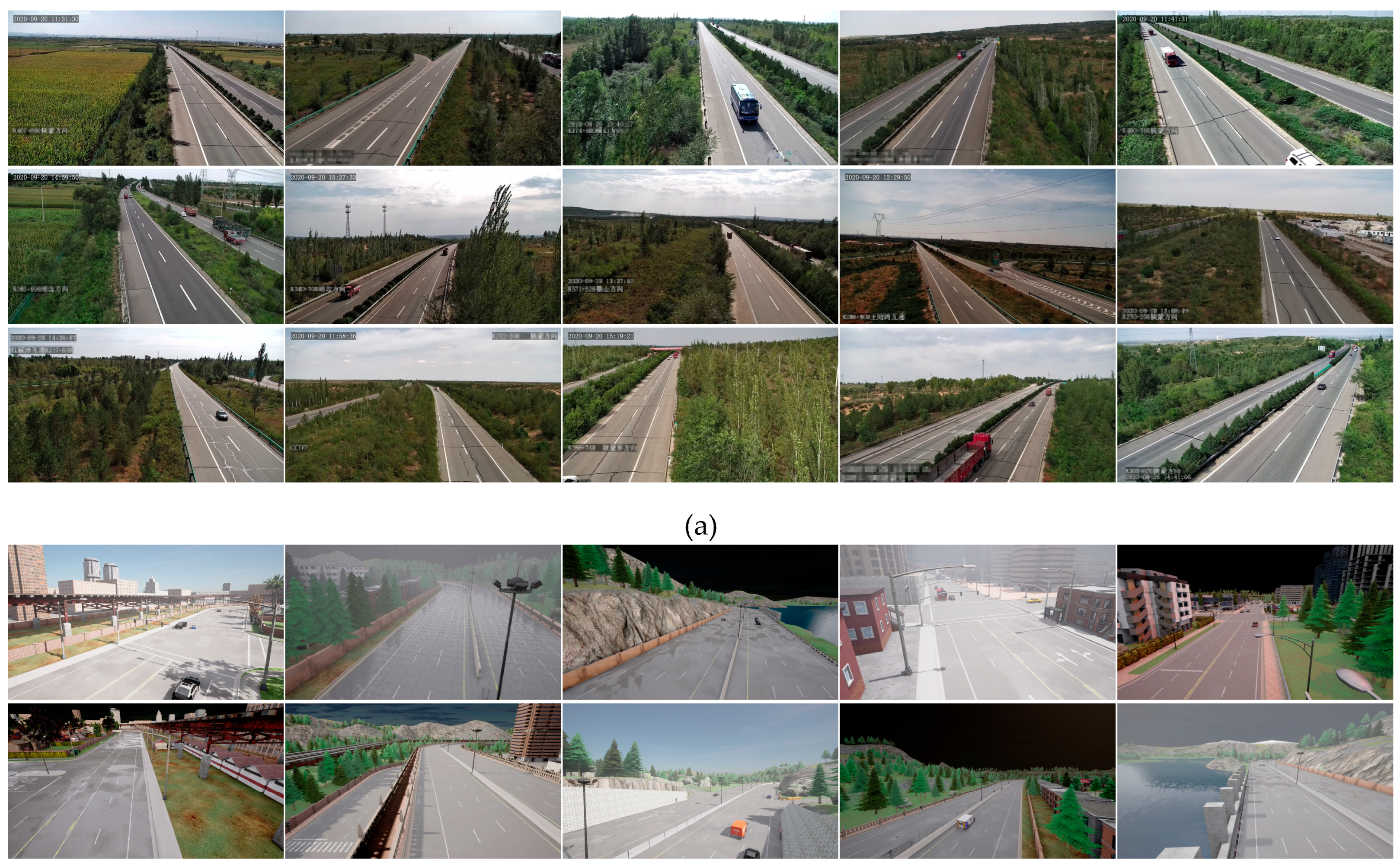
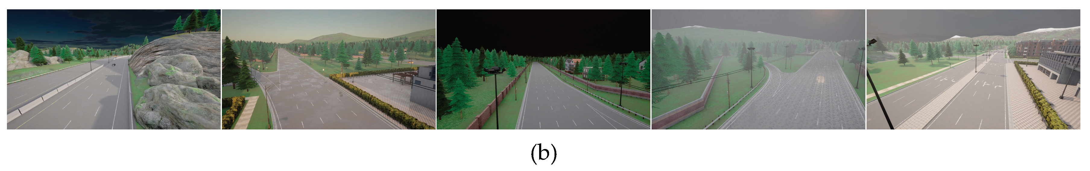
Figure 2.
Distribution of vanishing point coordinates in MVCCD_S.
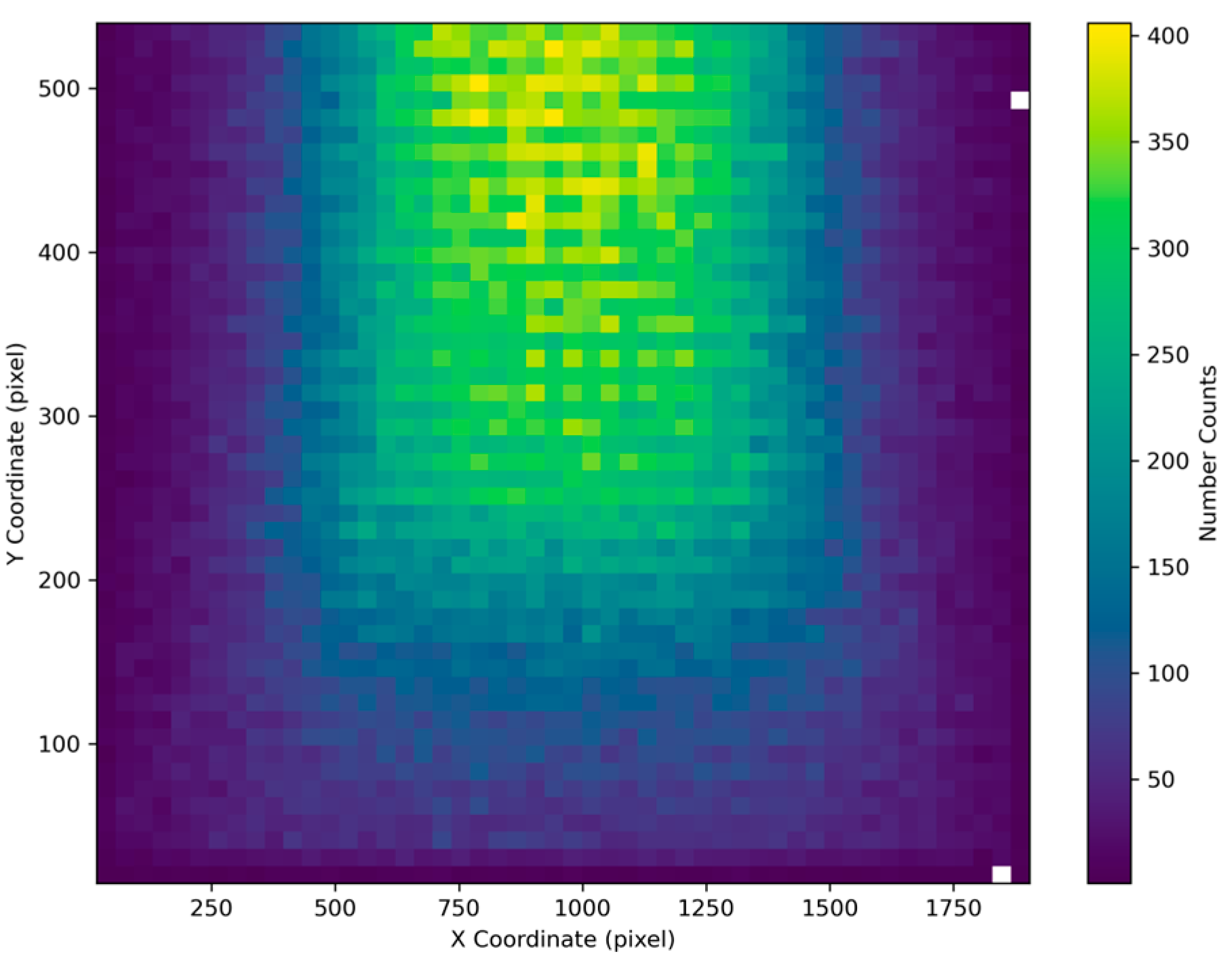
Figure 3.
Histograms of camera parameters in MVCCD_S.
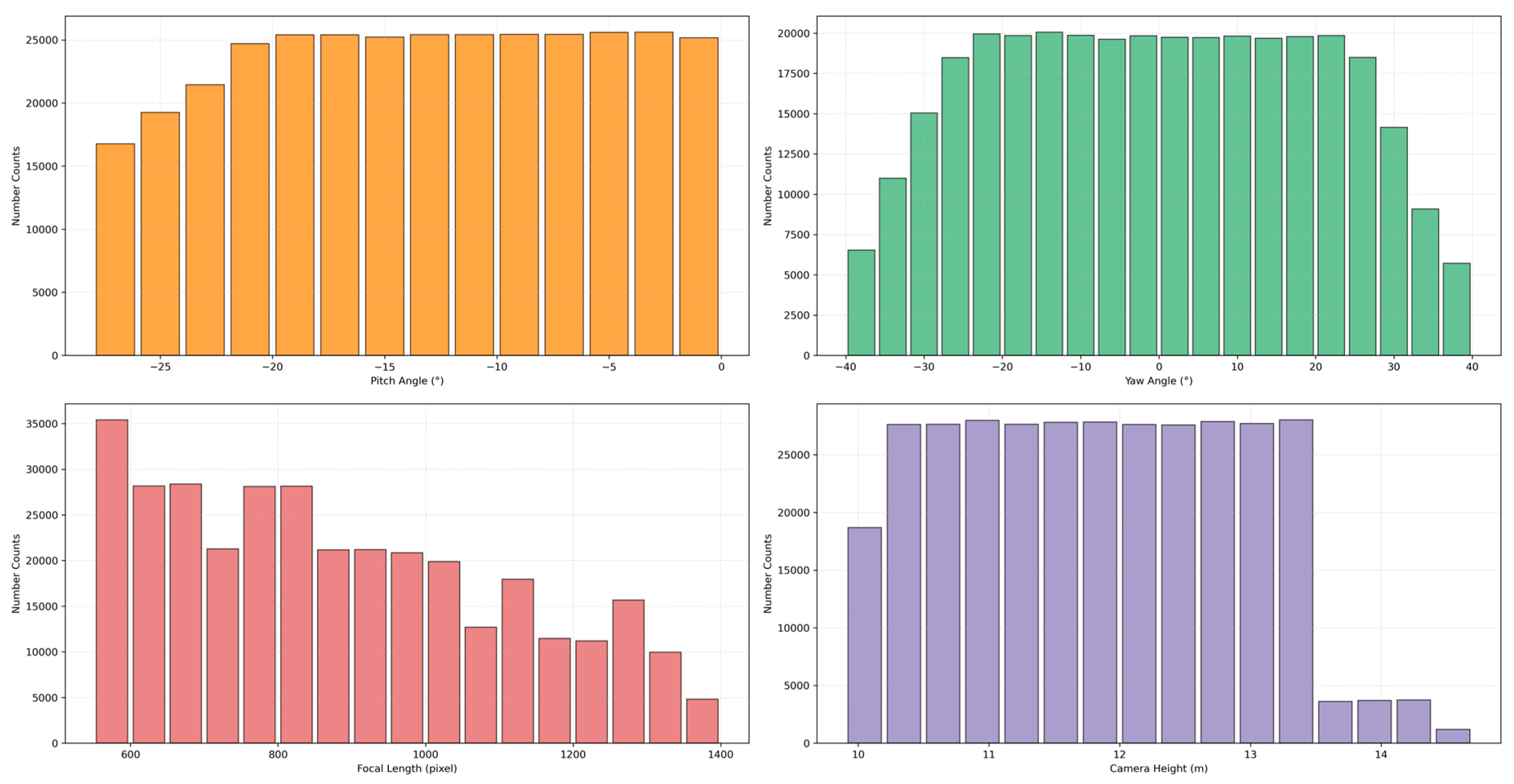
Figure 4.
Traffic surveillance camera calibration model. The camera is placed at a height of h meters above the ground plane. Xw-Yw-Zw axis represents the world coordinate system, while Xc-Yc-Zc axis represents the camera coordinate system. U denotes the vanishing point along the road direction.
Figure 4.
Traffic surveillance camera calibration model. The camera is placed at a height of h meters above the ground plane. Xw-Yw-Zw axis represents the world coordinate system, while Xc-Yc-Zc axis represents the camera coordinate system. U denotes the vanishing point along the road direction.
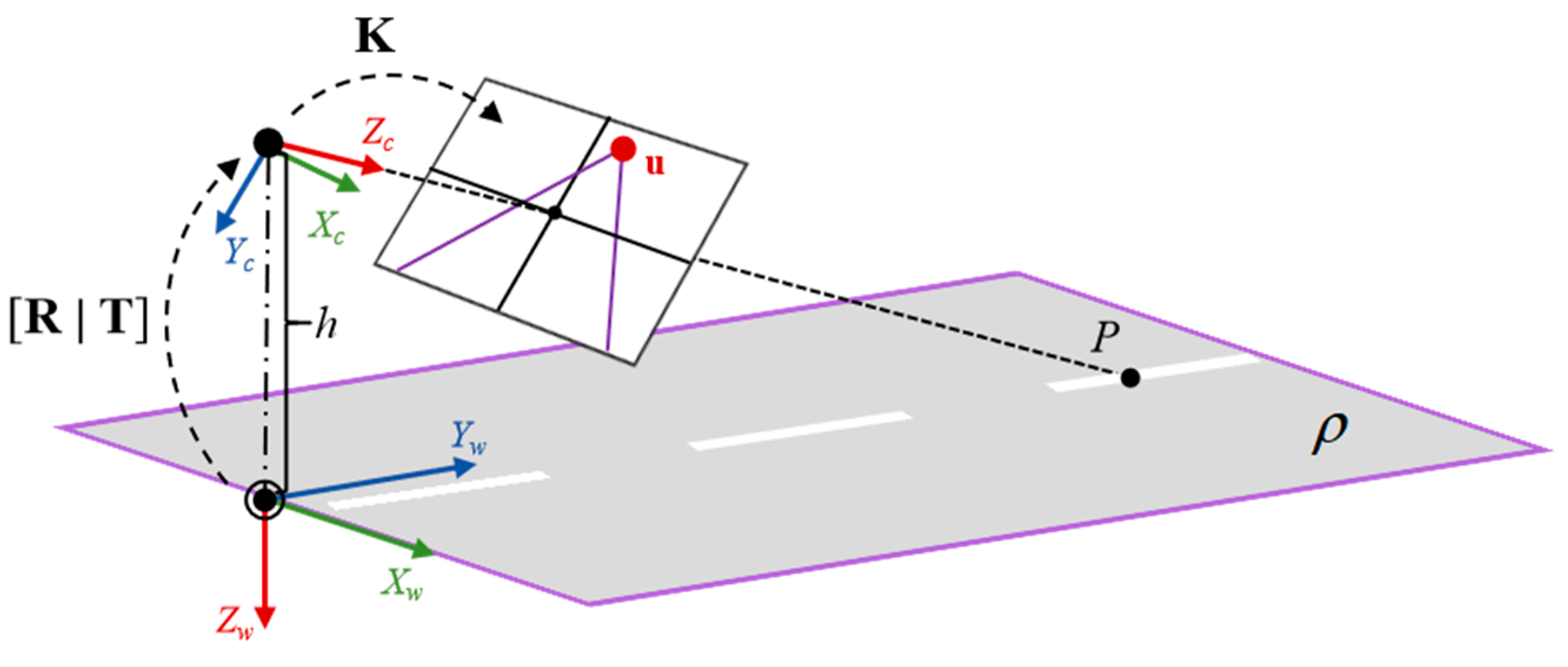
Figure 5.
The overall framework of DeepCalib. TAM stands for the triplet attention module. The symbol ⊕ denotes feature fusion and © indicates feature map connection. The keypoint branch outputs vanishing point heatmap, and the camera pose branch estimates extrinsic parameters.
Figure 5.
The overall framework of DeepCalib. TAM stands for the triplet attention module. The symbol ⊕ denotes feature fusion and © indicates feature map connection. The keypoint branch outputs vanishing point heatmap, and the camera pose branch estimates extrinsic parameters.
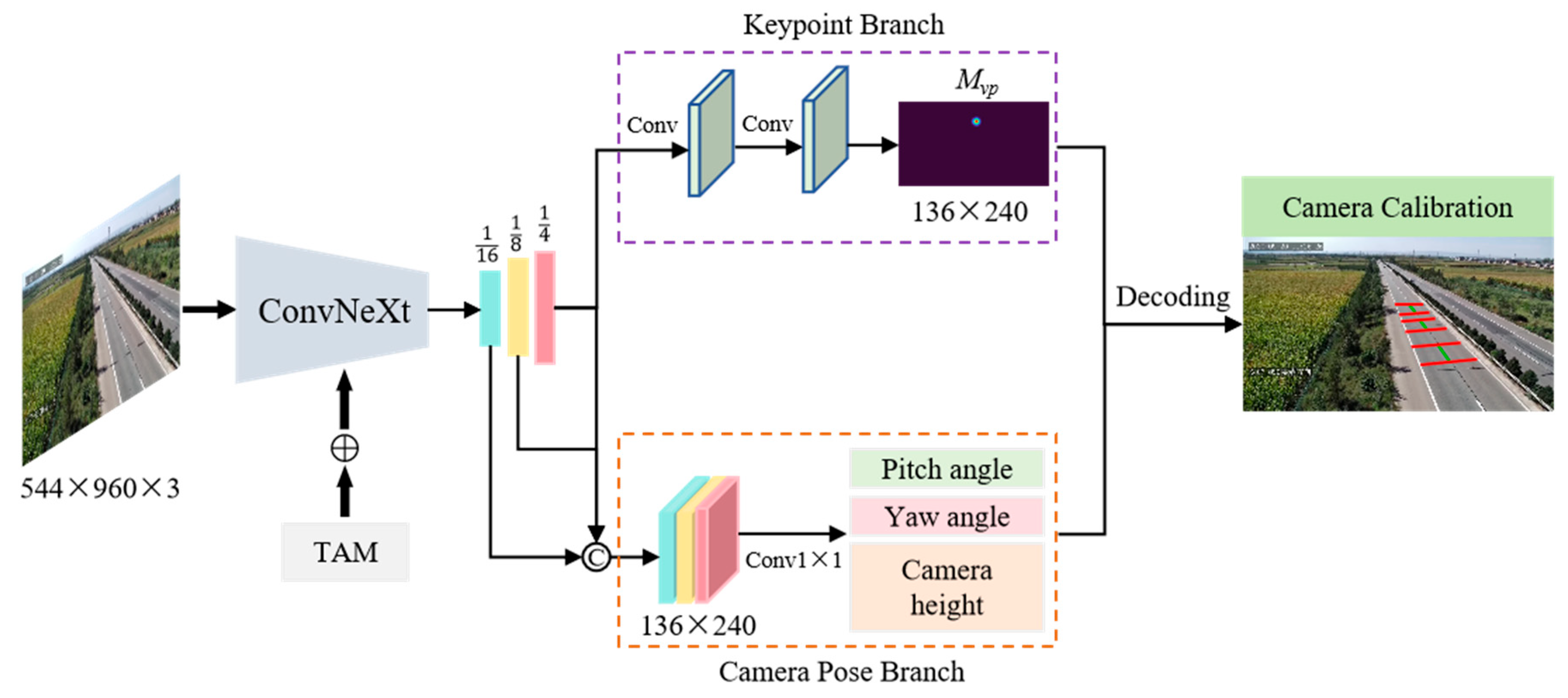
Figure 6.
Schematic diagram of rotation angle estimation.
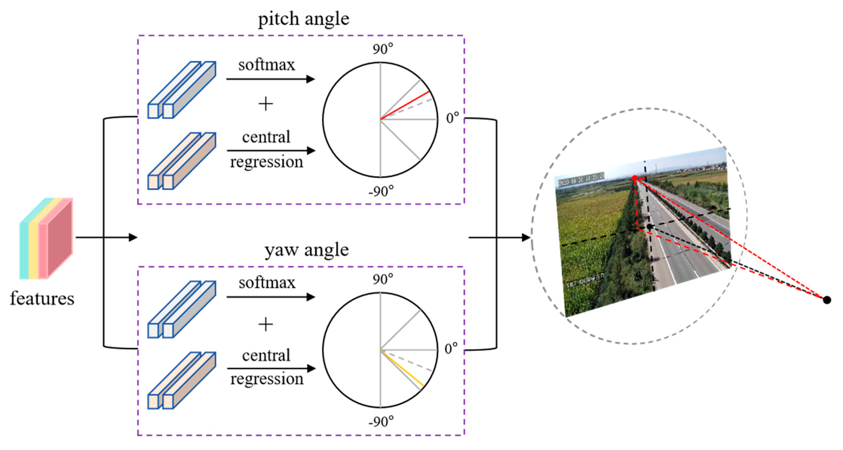
Figure 7.
Ablation study results.
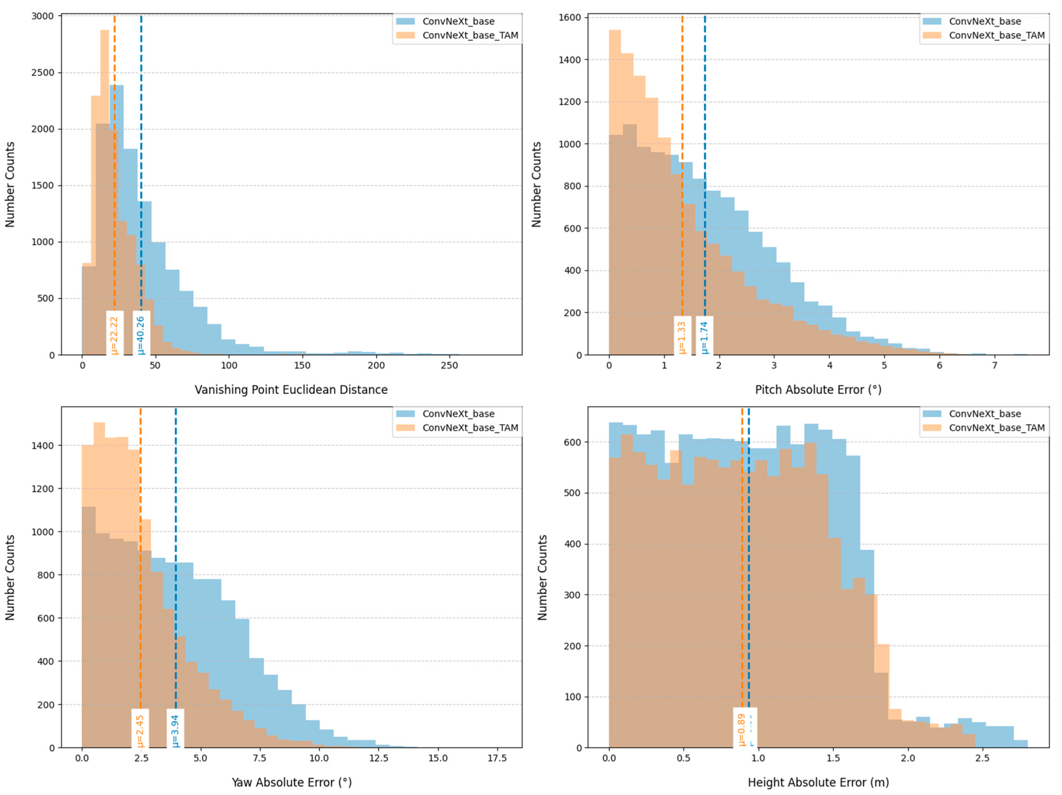
Figure 8.
Loss curves for direct training and transfer learning.

Figure 9.
Quantitative analysis of direct training and transfer learning.
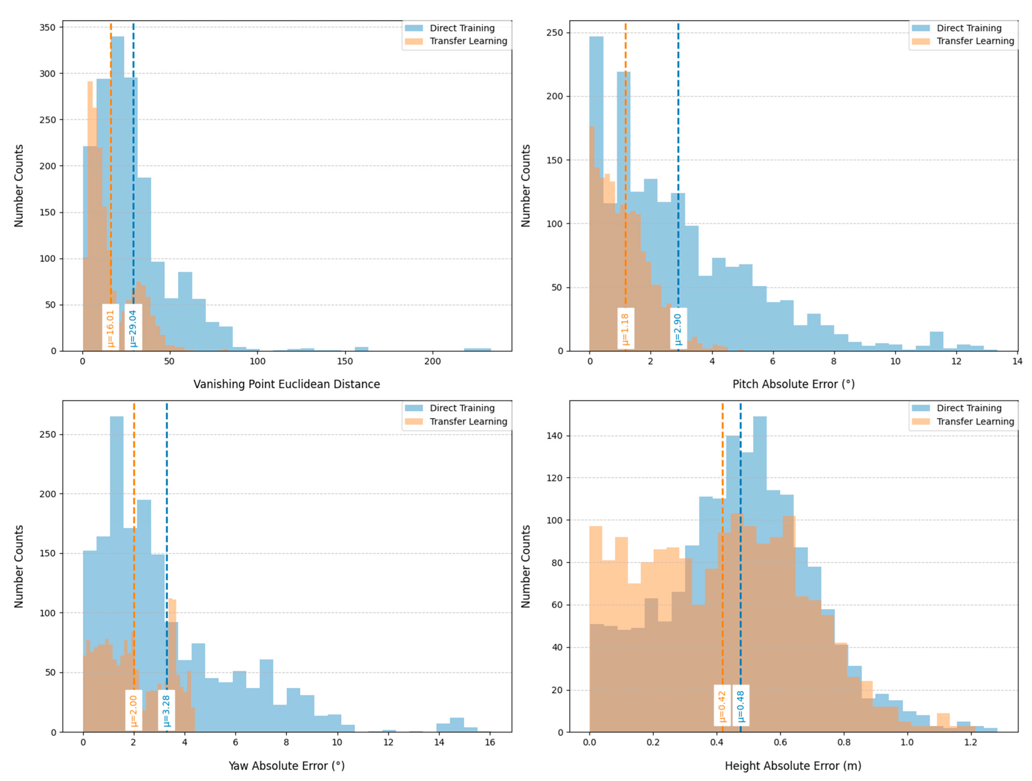
Figure 10.
Qualitative comparison of vanishing point detection performance by DeepCalib on real-world test images. (a) Straight road scenarios; (b) Curved road scenarios. For each row, the left image shows results from a model trained exclusively on MVCCD_R, while the right image demonstrates outcomes after pre-training on MVCCD_S followed by fine-tuning on MVCCD_R.
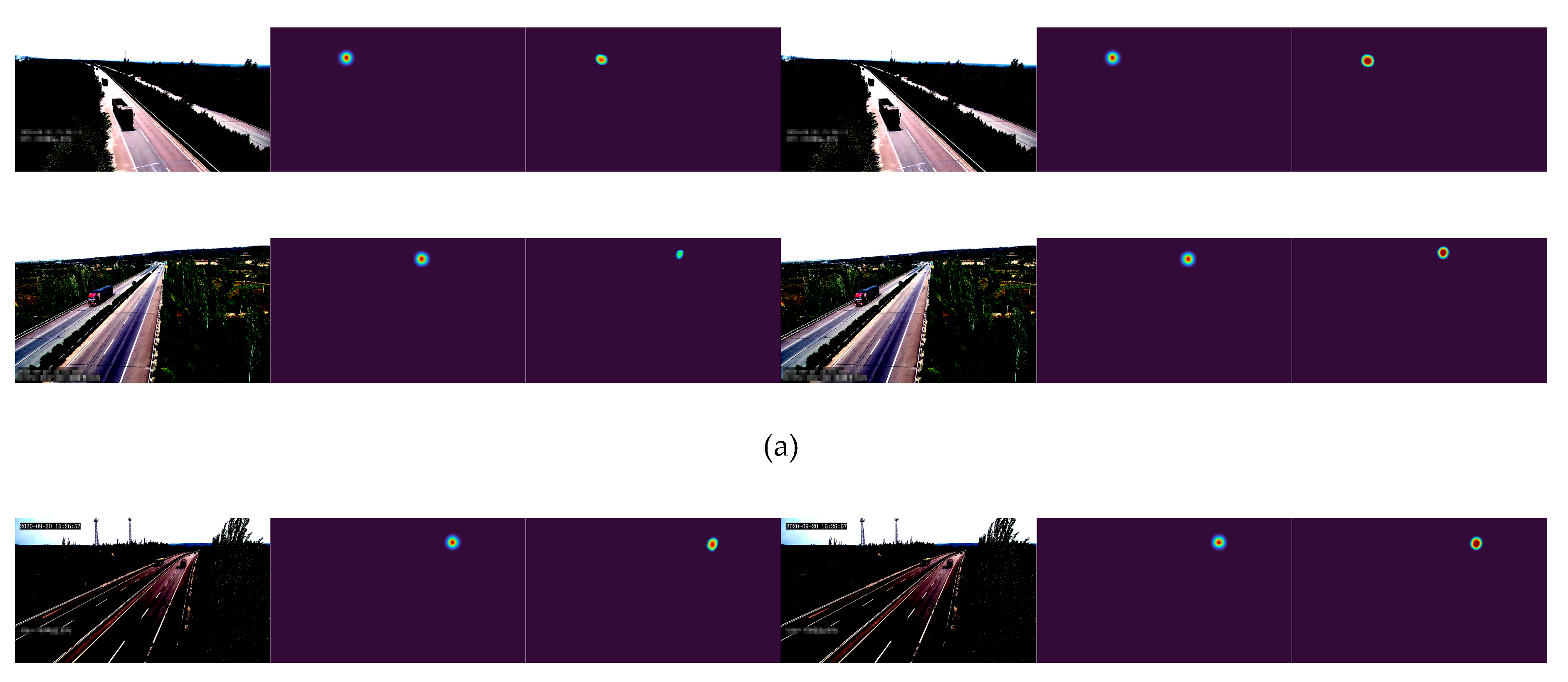
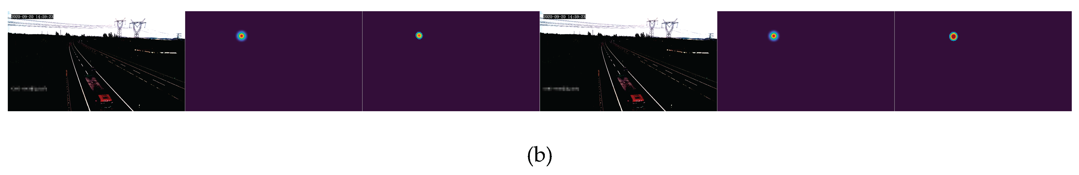
Figure 11.
Schematic diagram of three different measurement line segments on the lane.
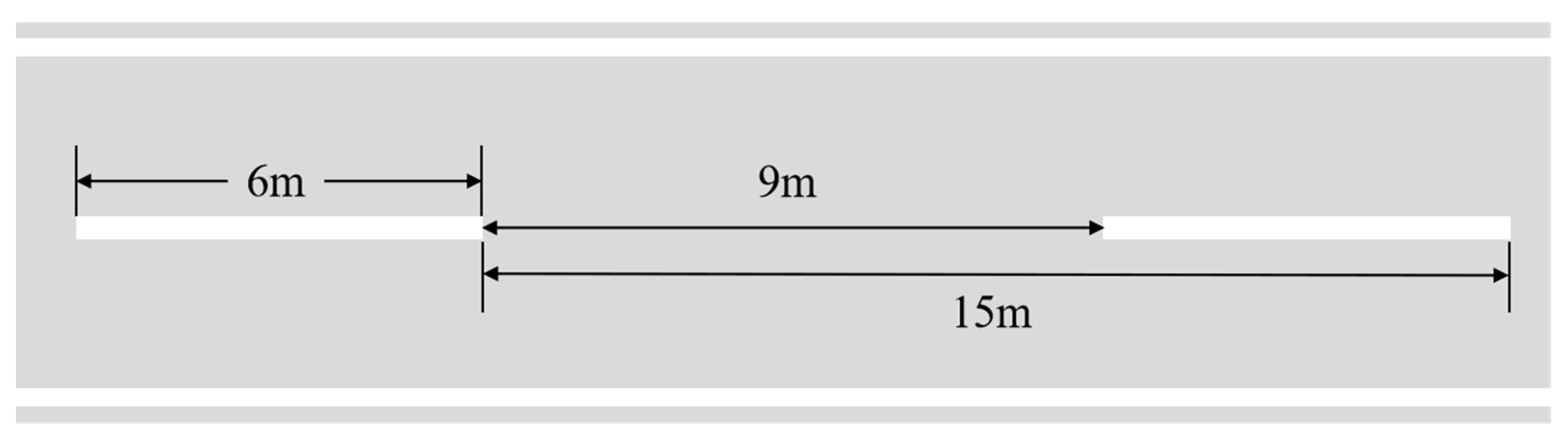
Figure 12.
Calibration results of the DeepCalib model in real-world scenarios. (a) Straight road environment; (b) Curved road environment.
Figure 12.
Calibration results of the DeepCalib model in real-world scenarios. (a) Straight road environment; (b) Curved road environment.
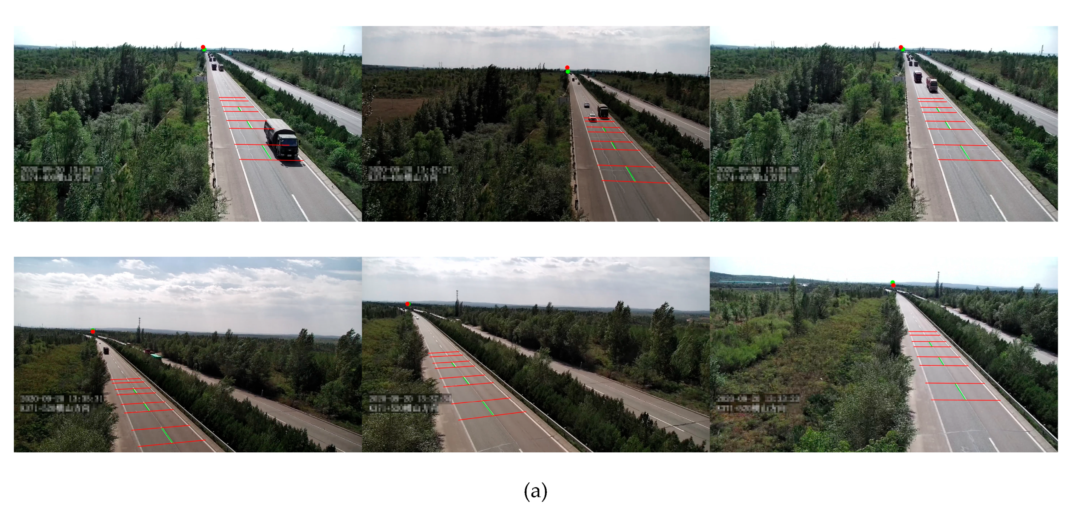
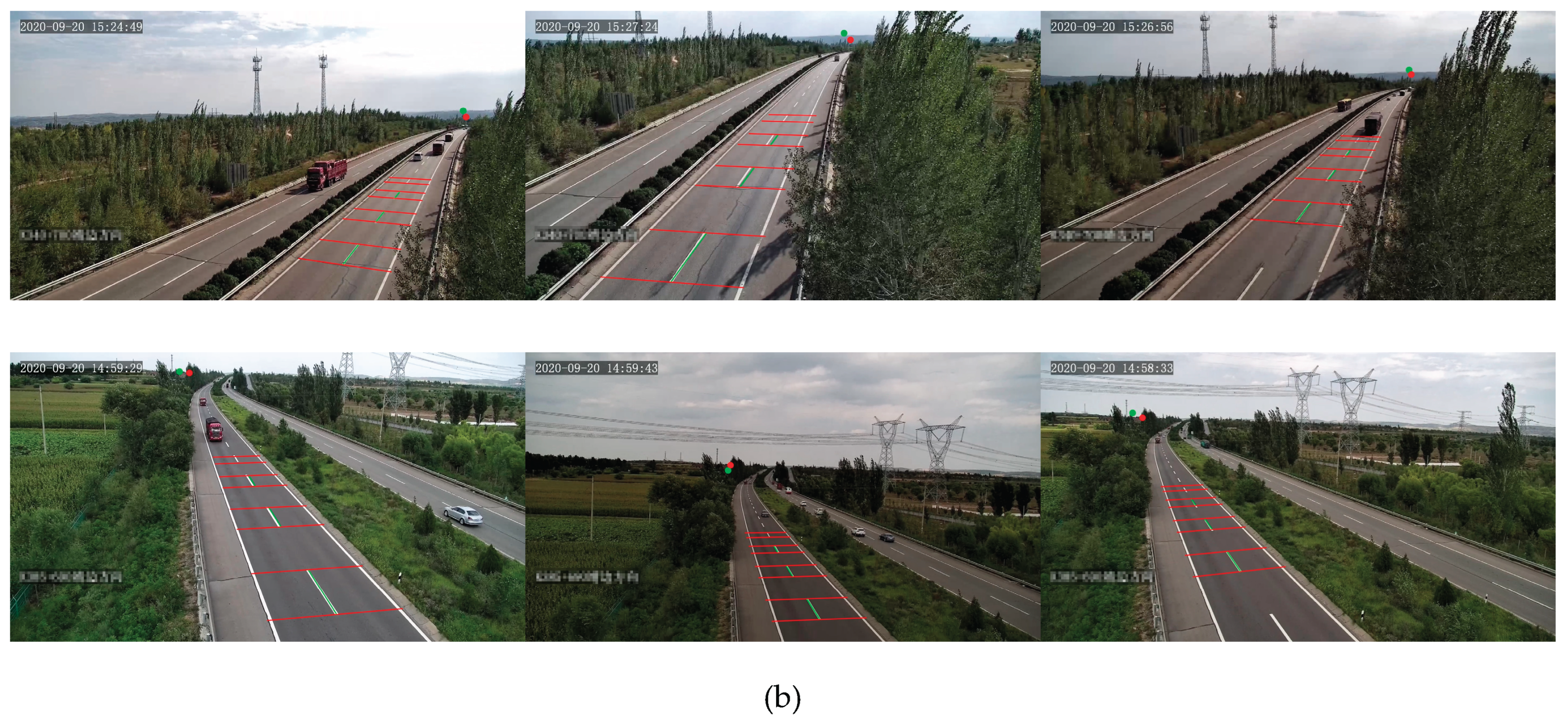
Figure 13.
Time consumption statistics for individual modules of the DeepCalib model.
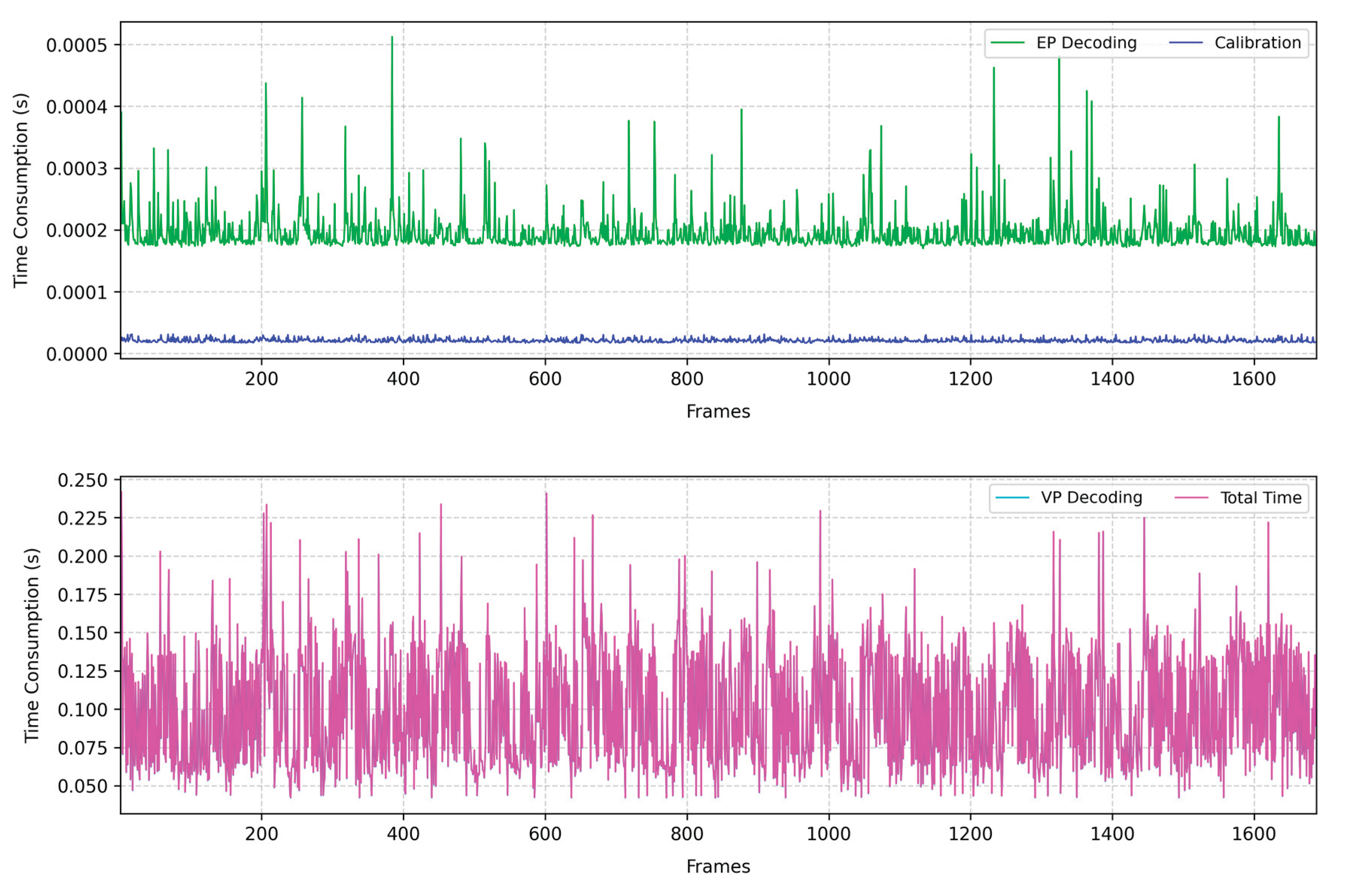

Table 1.
Comparison of the real-world and synthetic dataset parameters.
| Dataset | Sample Size | h | Format | Resolution | ||
| MVCCD_R [3] | 8,765 | [−18.4°, 0°] | [−29.3°, 29°] | [10.4m,13.9m] | RGB | 1920×1080 |
| MVCCD_S | 336,249 | [−28°, 0°] | [−40°, 40°] | [10m,14.5m] | RGB | 1920×1080 |
Table 2.
Comparison of vanishing point detection performance on straight and curved roads.
| Methods | Straight Roads | Curved Roads | ||||
| Minimum | Maximum | Mean | Minimum | Maximum | Mean | |
| DeepVP [27] | 8.58 | 235.22 | 91.08 | 20.39 | 336.06 | 119.43 |
| DeepCN [3] | 3.37 | 112.54 | 57.14 | 12.66 | 189.45 | 73.16 |
| DeepCalib | 1.34 | 58.73 | 13.11 | 7.07 | 79.21 | 34.29 |
Table 3.
Comparison of DeepCN, DeepCalib and manual methods for line segment measurement.
| Methods | 6m | 9m | 15m | ||||||
| Minimum | Maximum | Mean | Minimum | Maximum | Mean | Minimum | Maximum | Mean | |
| Manual | 5.87 | 6.22 | 6.05 | 8.53 | 9.09 | 8.91 | 14.71 | 15.15 | 14.96 |
| DeepCN [3] | 2.77 | 10.24 | 6.82 | 3.51 | 15.02 | 10.27 | 7.28 | 25.87 | 17.11 |
| DeepCalib | 3.44 | 9.18 | 6.56 | 4.77 | 14.94 | 9.96 | 9.05 | 23.43 | 16.68 |
Disclaimer/Publisher’s Note: The statements, opinions and data contained in all publications are solely those of the individual author(s) and contributor(s) and not of MDPI and/or the editor(s). MDPI and/or the editor(s) disclaim responsibility for any injury to people or property resulting from any ideas, methods, instructions or products referred to in the content. |
© 2025 by the authors. Licensee MDPI, Basel, Switzerland. This article is an open access article distributed under the terms and conditions of the Creative Commons Attribution (CC BY) license (http://creativecommons.org/licenses/by/4.0/).
Copyright: This open access article is published under a Creative Commons CC BY 4.0 license, which permit the free download, distribution, and reuse, provided that the author and preprint are cited in any reuse.


