
Submitted:
05 December 2023
Posted:
06 December 2023
You are already at the latest version
Abstract
Building deep learning models proposed by third parties can become a simple task when specialized libraries are used. However, a great deal of mystery still surrounds the design of new models or the modification of existing ones. These tasks require in-depth knowledge of the different components or building blocks as well as their dimensions. This information is limited and broken up in different literature. In this article, we collect and explain in-depth the building blocks to design deep learning models, starting from the artificial neuron to the concepts involved in building deep neural networks. Furthermore, the implementation of each building block is exemplified using the Keras library.
Keywords:
Deep learning
; artificial neural networks
; convolutional neural layer
; activation layer
; pooling layer
; forward propagation
; backpropagation.
1. Introduction
Artificial intelligence (AI) plays a vital role in successfully implementing Industry 4.0. Besides, in the last ten years (2013-2023), the leading branch of AI turned out to be deep learning (DL). DL is an important subfield of machine learning (ML) characterized by its layered structure of artificial neural networks (ANN). Each layer extracts helpful knowledge to make decisions or future predictions to solve self-supervised, semi-supervised, supervised, and unsupervised learning problems [1,2,3].
Currently, many industry sectors are experiencing a tremendous conversion and integrating DL models in their solutions [4,5,6]. For example, DL is used in the nuclear energy industry to predict cracking in hazardous areas. In the agriculture industry, DL is used to analyze historical rainfall patterns, wind direction, and atmospheric pressure to predict storms and river water levels [7]. In the manufacturing industry, it is used for predictive maintenance. In the food industry, it is used to understand current consumer preferences and behavior [8]. In the automotive industry, DL is used to guide autonomous vehicles [9]. In the medical industry, it is used to diagnose and predict illnesses [10,11,12]. The increase in popularity is mainly due to three factors: 1) the rapid evolution of the hardware with a highly parallel structure, 2) the development of open-source platforms for ML, and 3) the predominance of the DL models in terms of accuracy and flexibility to represent the world with concepts that range from the simplest to the most complex. All this is powered by a huge amount of data [13].
Despite this importance, DL models are considered black boxes whose components or building blocks are unclear and difficult to understand. Much of the research is based on the straight application of deep networks that have already been developed. The authors do not contemplate modifications and avoid discussing a new network design for a specific input signal type. Furthermore, the explanation of the building blocks to carry out new model designs or modifications to the current ones is limited, light, and dispersed in the different literature. In this paper, we describe the building blocks to construct DL models, from the main component, the artificial neuron (AN), to the formalization to analyze deep neural networks (DNN). Examples of implementations in Keras accompany all this [14].
2. Materials and Methods
In this section, the building blocks to design convolutional layers, pooling layers, and fully connected layers are discussed, commencing with the formalization of the main building block, which is the AN.
2.1. The Artificial Neuron
The AN is the backbone of deep neural network (DNN) algorithms and bases their operation on a collection of interconnected artificial neurons organized in layers, where each connection transmits a signal to the neurons in the next layer. Figure 1 represents an artificial neuron (also known as a unit), and to are learnable weights or learnable parameters. Furthermore, is the offset or bias that allows other influences to be included in the model, and is an input set permanently to 1, meaning that the bias is always on. The input features are to , and is the output of the non-linear activation function.
Two operations are conducted in an artificial neuron: 1) a linear combination of the input features with the weights or parameters w and 2) a non-linear mapping. The linear operation is expressed as,
The non-linear mapping is carried out by adding a non-linear activation function to process the linear combination z further and to approximate complex patterns. Then, the output moves to the succeeding layer through the next learnable weights. This process is known as forward propagation. Subsequently, a backward pass or backpropagation of the errors is performed to adjust the weights to correct errors and improve accuracy. The backpropagation is based on a gradient that requires continuously differentiable activation functions [15,16]. Table 1 shows some common activation functions.
The following code defines a nine-input neuron with bias and sigmoid activation function in Keras.
model = Sequential()
model.add(Dense(1, input_dim=9,
use_bias=True, activation=’sigmoid’))
2.2. Convolutional Layer
A convolutional neural network (CNN) is a type of DNN used for finding patterns in images to recognize objects, classes, and categories. This network performs a convolution operation of trained filters with the input signal to extract patterns. Each filter extracts a different pattern and forms a convolutional layer, the major building block of the CNNs. After training, the layers are able to extract patterns from the data without human intervention. The convolution operation consists of sliding trainable convolutional filters over the receptive field, producing a layer of features that indicates the strength and positions of the detected features. Besides, complex patterns are detected by adding activation functions to process further the filtered signal [17,18,19].
2.2.1. Convolutional Filters (Kernels)
The core of a CNN are the trainable filters, also known as kernels, whose weights or parameters are learned during the training process. The input to the filters is known as the receptive field that, convolved with the filter parameters, yields a set of feature maps that is further processed with activation functions. The output can be used as the receptive field for the next set of trainable filters used to extract a different set of features. The filter parameters depend on the characteristics of the input. They are trained to extract features from structures in the receptive field, such as vertical, horizontal, or diagonal edges. However, one filter can represent only a single structure. Hence, we must train multiple filters to represent multiple structures from a single receptive field.
Processing grayscale images of size requires two-dimensional (2D) kernel windows of height and width coefficients. Figure 2 shows the convolution process to obtain three features from a one-channel 2D receptive field. The lines represent the learnable parameters (weights) and the black dot, joining the lines, the sum of products of Equation (2) with and .
The pixels in the receptive field are multiplied by the parameters, and the result is added to yield one feature. The filter is slid row- and column-wise over a valid area of the receptive field by a factor S known as the convolution stride. After the convolution operation over the complete receptive field, one map of features is obtained. This map is also called a channel.
Observe that the filter coefficients convolved with values inside the valid area of the receptive field produce a feature map of smaller than the receptive field. To keep the same size, the receptive field must be padded around with P rows and columns of zeros before convolution. After the convolution operation, the resulting feature map is of size,
where is the floor operation. Three-channel receptive fields, such as the color images, are processed by programming one filter per channel. The filter outputs are added to produce a single feature map or channel. Notice that the number of channels is reduced from three to one while the number of parameters is multiplied by a factor equal to the number of channels.
Figure 3 shows the filtering process to extract one feature from a three-channel receptive field. Each filter carries out the sum of products inside their corresponding window. The three results are added to yield one feature. Afterward, the filter is shifted to the number of pixels defined by S. The three channels must be padded to keep the output feature map size equal to the receptive field.
Before training, the filter parameters are randomly initialized. One popular technique is the He initialization [20]. Here, the normal probability distribution is used with zero mean and standard deviation of , where is the number of hidden units in the previous layer .
During training, the feature maps are calculated and stored together with the parameters or learnable weights in the forward propagation step. The filter parameters are updated using the stored feature maps during backpropagation. Our example shows that the operation is a 2D convolution even though the filter moves over a 3D receptive field. The filter has the same depth as the receptive field and is shifted only along the rows and columns. The convolution does not occur along the depth, reducing the feature map to 2D.
One filter can extract features from only one structure of the receptive field. For example, if the extracted features belong to vertical edges and we want to extract features from other structures, we must add more filters. Therefore, each filter produces one channel or feature map. Hence, the resulting feature map can be seen as a volume of bi-dimensional feature maps with the number of channels (depth) defined by the number of filters utilized to produce the output volume.
Figure 4 shows an example of the convolution of a 3D filter of size over a valid area of a three channels receptive field of size samples each. The filters are represented as a 3D grid of trainable parameters to , and the bias term is omitted. According to Equation (3), the resulting 2D feature map is of size . The arrows point to the representation of the convolution in terms of volumes. The orange and yellow blocks are the volumetric representation of the receptive field and the filter respectively. Observe that the output is only one channel or 2D map of size .
If we add more filters, the number of output channels increases as shown in Figure 5, where three filters are convolved with a volumetric receptive field on a valid area of size to yield three feature maps or channels of size , represented by the green volume.
Convolutional filters possess two important characteristics: 1) parameter sharing and 2) sparsity of connections. Parameters sharing means that if a trained filter can extract certain features in one part of the receptive field, extracting the same features in another part of the same receptive field is also helpful. Therefore, the same weights are used for the kernel independently where the kernel is placed. Hence, each filter can use the same parameters in different positions in our receptive field. The sparsity of connections means that each feature of the feature map is computed using an area of samples (see Figure 5). The remaining values outside the area do not affect the output. These two mechanisms allow a model to be defined with a reduced number of parameters and to reduce the variance of parameters, reducing the possibility of overfitting.
It is important to highlight that the classical filters are handcrafted to produce a result such as detecting edges and removing noise. The difference with convolutional filters is that the parameters of the filters are learned during training by looking at the scene of a specific problem.
2.2.2. 2D Convolutional Layer
For the model to learn complex functional mappings, a layer of activation functions is required after filtering. In some cases, a bias term is added to the linear combination. Figure 6 shows the process of obtaining a 2D convolutional layer. Suppose the receptive field is a color image of size pixels. The convolution with three filters of size , over the valid area of the receptive field, with and will yield three feature maps of size each (see Equation (3)). This feature map is also called a map of activations or a convolutional layer. Moreover, to learn complex parameters, it is necessary to process the feature map further using an activation layer whose output is also called the convolutional layer. Therefore, the output volume of Figure 6 is called a 2D convolutional layer.
If we want the layer to be the same size as the receptive field, we use zero-padding P around the image before convolution. Figure 7 shows a portion of a receptive field padded around with one row and one column of zeros and three steps of convolution with a stride of one . The gray squares at the output of the activation layer represent the output features of the convolutional layer. For a color image, each channel must be padded, and the convolution operation must be carried out beyond the limits of the valid area of each channel. The activation unit shown represents a layer of activation functions and not only a single unit. Figure 8 shows the convolution operation with and .
CNN models add one convolutional layer after another to extract features from the previous layers. The greater the depth, the greater the complexity of the extracted features. However, the complexity of the model increases as the number of parameters increases. The number of parameters used in any of the layers can be calculated as,
where l is the current layer number, is the previous layer number, is the number of parameters in the current layer, the number of channels in the current layer and the number of channels in the previous layer. The dimension of a convolutional layer can be determined by using Equation (3). For example, if the input image is of size , grayscale, the filter size is , the stride is one, and no padding is used, the dimension of the output feature map is,
Hence, the dimension of the layer is . Observe that the number of parameters is determined by the number of weights of the filter plus the bias if it is used. According to Equation (4), the total number of parameters is (. Figure 9 shows an example of obtaining a convolutional layer after the convolution operation of the receptive field with a filter and the activation layer. The size of the convolutional layer is determined by Equation (5).
One filter is insufficient to capture most of the features in a receptive field. Hence, multiple filters must be used to create multiple feature maps, as shown in Figure 10. The gray shade grids represent the filter coefficients. The receptive field is convolved with four filters. Each output is passed through an activation layer to yield a convolutional layer of size,
Below is a piece of Keras code utilized to implement a two-layer CNN. The first layer accepts 2D receptive fields of size and learns 32 convolutional filters of size with bias term. The convolution is carried out over a padded area with a convolution stride of 1 along rows and columns. The activation map is passed through a ReLU activation layer to remove negative values and produce a convolutional layer of the same size as the input receptive field. This layer is the receptive field of the next layer. The second layer learns 64 filters of . The convolution operation is performed over a valid receptive field area, followed by a ReLU activation layer.
model=Sequential()
model.add(Conv2D(32,(3,3),padding=’same’,
strides=(1,1), activation=’relu’,
kernel_initializer=’he_normal’,
input_shape=(28,28,1)))
model.add(Conv2D(64,(5,5),padding=’valid’,
strides=(1, 1),activation =’relu’,
kernel_initializer=’he_normal’))
2.3. 3D Convolutional Layer
Three-dimensional (3D) convolutional neural networks are mostly used in 3D data. Such as Positron Emission Tomography (PET) Imaging, Magnetic Resonance Imaging (MRI) and Computerized Tomography (CT) Scan [21]. Typically, 3D architectures use the 3D convolution operation to extract features from three dimensions data. 3D convolutions apply three-dimensional filters to the data. The kernels may not be the same depth as the receptive field. For example, filters could be smaller in size than the input image.
Figure 11 shows the convolution of a volumetric receptive field (voxels of a 3D image) of size () with a filter of size (). The feature in the color blue is obtained by adding the sum of products inside the volume engulfed by the 3D filter in the receptive field (orange color). The filter is shifted by the number of voxels defined by S, and the calculation is repeated to compute a new feature. The size of the output volume depends on the values of P and S. The 3D CNN layer is obtained after a 3D activation layer.
Dimensions of the output volume are related to the dimensions of the previous volume by Eq. (6).
where is the height of the input volume. The width and depth of the volume are calculated similarly. Feature maps often increase with the depth of the network, which can result in a considerable increase in the number of parameters. As a result, the computation complexity is exacerbated when filters of larger sizes are used (, , etc.).
Following is a piece of Keras code to implement a two-layer model. The input shape () has four dimensions. The fourth dimension is the number of input channels. The input data is sized (). The layers learn 16 and 32 filters with kernel sizes of and , respectively. The parameters are randomly initialized [20]. Finally, the extracted 3D feature maps are passed through a 3D ReLU activation layer.
model = Sequential()
model.add(Conv3D(16,(5,5,5),padding=’valid’,
activation=’relu’,
kernel_initializer=’he_normal’,
input_shape = (16,16,16,3)))
model.add(Conv3D(32,(3,3,3),padding=’valid’,
activation=’relu’,
kernel_initializer=’he_normal’))
The number of parameters learned in the first layer is and the layer size is . This layer is the receptive field of the second layer. The second layer learns parameters, and the output layer is of size , where the fourth dimension is the number of channels yielded. In both layers, the convolution operation is performed on the valid area of the receptive field. Therefore, the dimension of the convolutional layers is smaller than its receptive field.
2.3.1. 1×1 Convolutional Layer
Stacking convolutional layers is computationally expensive and prone to overfitting. A strategy to reduce the complexity is to apply convolution to multi-channel receptive fields. It is implemented using filters of size , where D is the depth of the receptive field. The convolution is carried out along rows and columns of the volume, creating a linear projection of a stack of channels or feature maps. Hence, the output is a feature map with the same spatial dimension as the receptive field with the number of channels D collapsed to one, as shown in Figure 12. It does not make sense to apply convolution to a single-channel receptive field because, in this case, the convolutional filter consists of one coefficient only [22].
The convolution layer can be added to a model architecture in Keras as follows,
model.add(Conv2D(16,(1,1),use_bias=False,
activation=’relu’,
kernel_initializer=’he_normal’,
input_shape=(256,256,3)))
The layer processes three channels input of size . The bias factor in each filter is not used. Hence, the number of parameters is 48. The output layer is a volume of dimension .
Figure 13 shows an inception module of the GoogLeNet or Inception V1 network [23] that uses three filters ( and ), one Max Pool operation and one concatenation layer. The convolution is implemented with a stride of one () yielding and the output layer keeps the same size ( ’’ ) as the receptive field.
Suppose we want to obtain a convolutional layer, similar to the yellow block in the second branch of Figure 13. Furthermore, assume we do not use the 96 filters of size in the middle. Therefore, we must use 128 filters of . Hence, we carry out a total of multiplications. On the other hand, if we insert the middle block, the number of multiplications is reduced to .
2.4. Polling Layer
After the activation layer, the convolutional layer contains the precise position of the features. Hence, if small movements in the receptive field occur, the resulting features change. This problem has been addressed in signal processing by using the so-called downsampling operation, which is carried out by using a stride different from one during the convolution operation to keep important features and discard details that may not be useful. A similar operation is carried out by adding a pooling layer after the activation layer [24]. However, in the convolution operation, some generative models replace this layer with a stride different from one.
The pooling layer reduces the spatial resolution of a feature map and provides limited invariance to rotation and small shifts. Pooling acts on a convolutional layer separately to create a reduced set of feature maps and to lower the memory requirements. The main mechanisms used by this layer are Max Pooling, Average Pooling, and Global Pooling, which are explained below.
2.4.1. Max Pooling and Average Pooling
Pooling operations are applied on a fixed-shaped window, known as a pooling window, that is shifted in the feature map according to its stride and computing a single value in each window location. Max pooling preserves the maximum value inside the windows, and average pooling preserves the average value inside the window.
Figure 14 shows the max pooling operation on a valid area of a receptive field, without padding and with a stride of one and two, respectively. The red square represents the initial pooling windows. Notice how the window pools the four values into one.
Figure 15 shows the average pooling operation with strides of one and two, respectively. The output is the reduced feature map or max pooling layer. Notice that when , each resolution is halved, reducing the number of values in each feature map to one-quarter the number of values in the receptive field.
Pooling in 3D is carried out upon a volumetric receptive field by extracting the maximum or the average value in a window of size that moves along x, y, and z axis. A pooling layer can be added after a convolution operation carried out with a stride equal to one , to reduce the size of a feature map.
More complex feature maps can be extracted using the convolutional layers as the receptive field of another set of filters. Hence, we can stack several layers by extracting features from previously generated layers. This process is called a hierarchical representation of features because the initial layers detect simple patterns like edges, and the higher layers detect more abstract features. Max Pooling layer with a windows size of and stride of 2 can be added to a model as follows,
model.add(MaxPooling2D(pool_size=(2,2),
strides =(2, 2)))
and the average pooling layer as,
model.add(AveragePooling2D(pool_size=(2,2),
strides =(2,2)))
2.4.2. Global Pooling
Global pooling reduces the entire feature map into a single sample. This mechanism is utilized as an alternative to a fully connected (FC) layer. It consists of converting the entire feature maps to a single output prediction that sums up the presence of a feature in a feature map. Global pooling can be performed by a global average pooling operation, which consists of taking the average of the entire feature map, or the global max pooling operation, which takes the maximum value of a feature map. The resulting values of the global pooling operations are applied to each feature map. The resulting vector can be applied directly into the softmax layer in the case of multiclass classification. Some advantages of global pooling are that it is more robust to spatial translation of the receptive field, there are no parameters to optimize, and it is more native to convolution structure because there is a direct correspondence between feature maps and classes. One example of global pooling is the inception network that uses the global average pooling operation after the last inception module instead of FC layers.
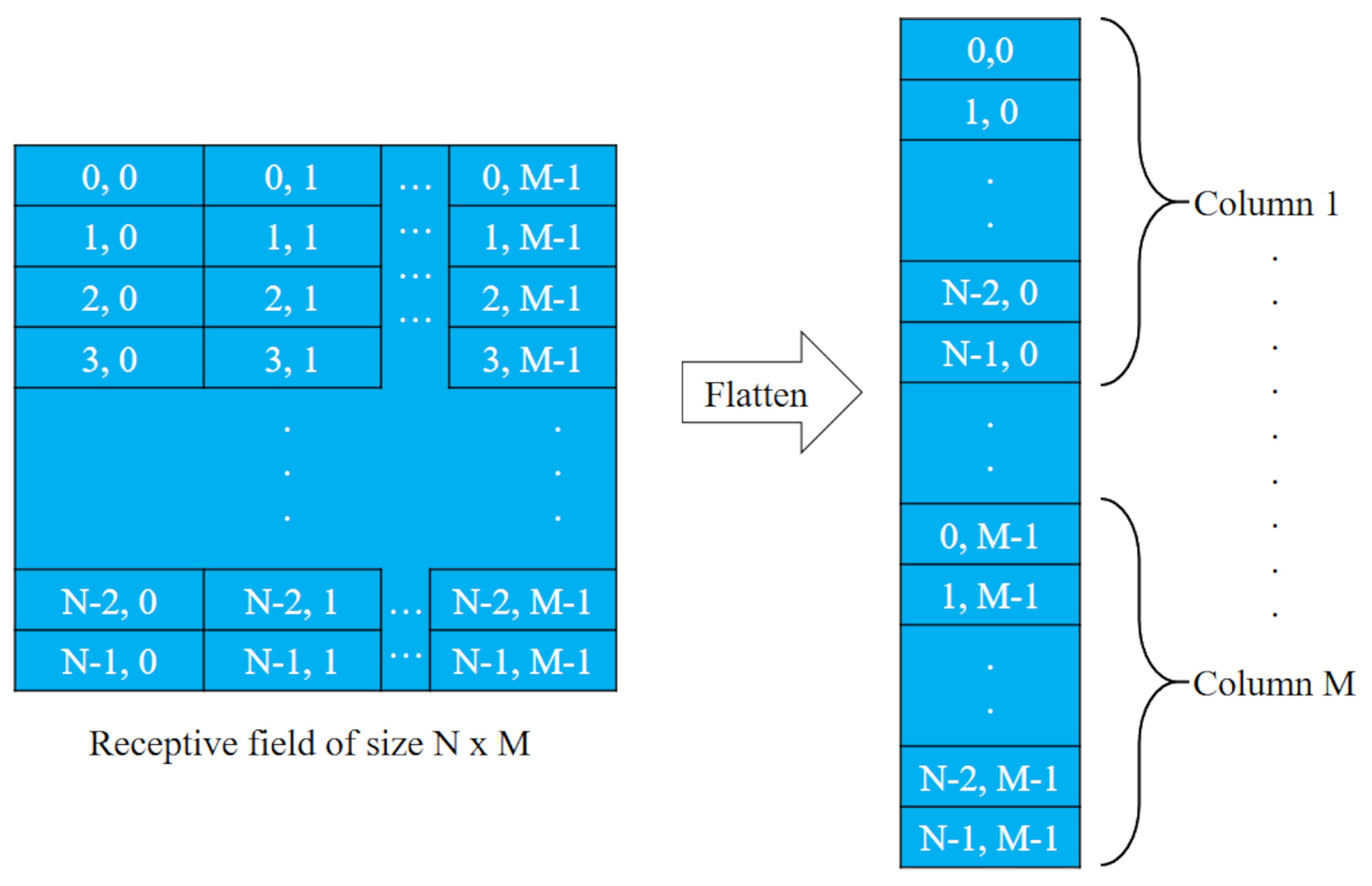
2.5. Flattening Layer
In classification models, the last stage is built of fully connected layers. Hence, the input must be a one-dimensional linear vector. If the input to the fully connected layer has a different dimension, it has to be converted into a one-dimensional array to create a single feature vector. This process is known as flattening. Figure 16 shows the process of flattening a two-dimensional receptive field. It consists of concatenating the receptive field column by column (or rows by row) one after the other to obtain a one-dimensional vector of size . In Keras, a flattened layer can be added using the function,
model.add(Flatten())
Figure 16.
Flattening by columns of a 2D receptive field.
2.6. Fully Connected Layer
Figure 17 shows a four-layer shallow network. The lines are the weights conveying information from one layer to another in the direction of the arrows. The green, blue, and orange circles represent the input, hidden, and output units, respectively. The white circles are the bias units. Notice that the output units from a previous layer are connected to every layer in its preceding layer. This type of layer is known as the dense or fully-connected layer (FC) layer.
Typically, the ANNs are built with one or more FC layers. The computations are carried out using vectorized algorithms. However, when building ANN models, one frustrating problem is obtaining the correct shape of the vectors and matrices of each layer. Even when using software like Keras [14], Caffe [25], or PyTorch [26], model design can result overwhelming if the dimensions of each layer are not considered. In this section, we explain how to calculate the dimensions of the matrices and vectors of FC layers.
Here, we introduce the superscript to denote the layer and the subscript j to denote the unit number in the layer. Therefore, the notation denotes the linear combination operation of the neuron, located in the layer. Hence, Equation (1) can be modified as,
Let us review the modeling of an ANN. Our goal is to describe the network by finding the equations that define the forward propagation from the input to the output layer. We first construct the input vector in , also known as feature vector or input example. The weights connecting the input features with each hidden unit can be placed in a column vector to end up having a total of the column vectors, where is the number of hidden units in layer 1. Consider the weights matrix mapping the input vector from the layer to the layer with rows being the set of transpose vectors and the bias vector the set of weights . Then, the linear combination in the first layer is the vector and the activation output is .
By letting the output of some activation function, we can express the forward propagation equations of the network in terms of the input example as,
The dimension of the weights matrix is the number of neurons in the current layer l multiplied by the number of neurons in the previous layer . The dimension of the bias vector , the linear combination vector , and the output vector is the number of neurons in the current layer multiplied by one . Eventually, we can calculate the number of parameters as .
Observe the similarity of Equations (8) and (9) with the process shown in Figure 6. Analogously, we can say that the receptive field is the input image , are the filter coefficients, are bias terms and is the activation layer. Therefore, is the output volume convolutional layer, which can be the input or receptive field to the next layer.
The following code implements the sequential model of Figure 17 using Keras software, assuming that the network accepts 50 inputs, the two hidden layers have 32 nodes each with ReLU activation function, and the output layer has ten nodes with the softmax activation function. The weights are initialized using the He algorithm with normal distribution.
model=Sequential()
model.add(Dense(32,use_bias=True,
activation=’relu’,
kernel_initializer=’he_normal’,
input_shape=(50,)))
model.add(Dense(32,use_bias=True,
activation=’relu’,
kernel_initializer=’he_normal’))
model.add(Dense(10,activation=’softmax’))
2.7. Deep Neural Networks
Deep neural networks (DNN) are composed of many layers that allow for increasing the performance in the accuracy of the model. However, the greater the number of layers, the greater the computational complexity. Hence, using loops during training to iterate over all the input examples in the data set makes the process very slow. Therefore, vectorization is an important strategy to help improve the time performance of a DL model.
Consider the matrix with columns being a subset or the complete data set of m input vectors . Equations (8) and (9) can now be generalized in matrix form as,
where and . When , then is considered the output of the prediction model. Figure 18 shows a DNN with L dense layers. The units or neurons are grouped into layers as follows: the green circles represent the input features, the blue ones are the hidden units in hidden layers, the white ones are the biases of each layer and the orange circles are the units belonging to the output layer. The arrows indicate the flow of information from one layer to the next throughout the parameters. For binary classification, the last layer has one activation function, typically the sigmoid function, and for multiclass classification, it could be a layer with softmax functions.
In supervised learning, the data are labeled, meaning that, for each input example, there is a label that indicates to which class it belongs. Therefore, we can consider the matrix whose columns are the set of m vectors with the number of output labels per vector.
After forward propagation, we measure how the model is performing concerning the training set by using a cost function which depends on the parameters we wish to adjust. The goal is to minimize the cost. For this, we measure the variation of the cost concerning the variation of the parameters and from the last to the first layer to update such parameters with the appropriate values that minimize the cost function,
where is a column vector of ones. In other words, we want to find the best parameters such that the cost function is minimum,
The cost is the average loss over the entire training dataset. For example, in binary classification, the loss function is the cross entropy denoted by,
where ⊗ is the element-wise product operation. Often we want to predict a continuous value function instead of ‘1’ or ‘0’. Then, we have to use the mean squared error (MSE) as our loss function to measure the divergence between the predicted and the true output.
We can use the backpropagation algorithm with gradient descent or any variant, such as stochastic gradient descent with momentum, RMSprop, Adam, etc., to minimize Equation (13) [27]. The following equations are used to update the parameters provided that is given, where is the partial derivative of the cost with respect to . For one input example . Then is the vector of all derivatives . By letting , , , we can easily calculate the update equations as follow,
Then, we update the parameters using the gradient descent [16] with an adjustable learning rate .
Let us assume binary classification, then . Notice that and .
2.8. Comments on Training DNN
For a large number of input vectors, we can split the data set into K subsets of data called minibatches with M examples each. Therefore, the set of minibatches are the matrices . In supervised learning, each minibatch is composed of pairs of training vectors. Each pair contains an input example vector and its truth output label or target output.
This technique is useful for huge training sets because it allows us to observe the progress of the model with each training minibatch before processing the entire training set, i.e., it allows us to take one gradient descent step with each minibatch. Also, to make the learning process fast, it is recommended to normalize the input features and the activations in each layer of the network.
During training, underfitting and overfitting must be avoided so that the network can correctly generalize new examples. Underfitting occurs when the network has not been trained for enough time or the number of parameters is not enough to establish the correct relationship between input and output variables. Underfitting is avoided by increasing the training time and/or increasing the number of model parameters. The overfitting problem is common when considering DNN because of the huge amount of parameters in the model. There are strategies to avoid overfitting. For example, we can employ data augmentation strategies such as random cropping, mirroring, rotating, and flipping the input data. In addition, we can add a regularization term to the loss function. Equation (17) shows the most common term of regularization known as -norm, weight decay, or Ridge Regression. It is nothing but the Euclidean norm of the weight matrices. Observe that, as the value of increases, the weights approach zero. This tends to cancel neurons, which reduces the number of parameters.
The Lasso Regression or -norm is another regularization technique that uses the absolute values of the weight parameters as a regularizer as shown in Eq. 18.
A similar effect can be seen when the dropout technique is used. During training, some of the outputs of some layers are probabilistically ignored (dropped out). Hence, these layers have a reduced number of units and reduced connectivity to the next layer, which means that the number of parameters is reduced, which prevents overfitting. The effect is similar to regularization. The following Keras code implements the neural network discussed in Section 2.6, using a dropout of 0.25. The architecture is configured to use the categorical cross-entropy loss function and the stochastic gradient with momentum and a learning rate of 0.01. The metric used to monitor and measure the performance of the classification model is ‘accuracy’. Finally, during training, the model is going to iterate the data ( ) with 40 epochs in minibatches ( ) of 8 input vectors each with their corresponding labels. There are three dense layers. However, only the middle one has a regularizer. Notice that the expression keras.regularizers.l2(l =0.01) denotes the regularizer with regularization parameter .
model = Sequential()
model.add(Dense(32, activation=’relu’,
kernel_initializer=’he_normal’,
input_shape=(50,)))
model.add(Dropout(0.25))
model.add(Dense(32, activation=’relu’,
kernel_initializer=’he_normal’,
kernel_regularizer =keras.regularizers.l2(l =0.01)))
model.add(Dropout(0.25))
model.add(Dense(10, activation= ’softmax’ ))
opt = SGD(lr=0.01, momentum=0.9)
model.compile(loss=’binary_crossentropy’,
optimizer=opt, metrics=[’accuracy’])
model.fit(data, labels, epochs=40, batch_size=8)
2.9. Tensors
Even though tensors are not a building block for deep networks, they are important since the input to deep learning-based models requires a large amount of high-dimensional data, and tensors are special containers for this kind of data. Tensors are able to store multidimensional arrays with uniform types. For example, a 0-dimensional tensor stores a scalar with zero axes and rank zero. An array is a 1-dimensional tensor for data of the same type, with one axis and rank one. A matrix is a 2-dimensional tensor of rank 2 with two axes. In general, an n-dimensional tensor is a tensor of rank n. An axis is a specific dimension and the length is the number of indexes available along that axis [28].
Figure 19 shows six tensors. We have tensors of 0-, 1-, 2-, and 3 dimensions in the upper part. The 2-dimensional tensor can be used to contain a grayscale image. The 3-dimensional tensor can be used to contain a color image or a color filter. The first dimension of the tensor expresses the number of channels. However, this dimension can be used to signal n different 2-dimensional matrices, which could be n grayscale images. This type of tensor is used to store a batch of images. The first dimension indicates the batch size. In the lower part of Figure 19, we see 4- and 5-dimensional tensors. A 4-dimensional tensor may contain color images, chunks of color images, or, in the case of a volumetric receptive field, hold the entire volume or small pieces of the volume.
The following Keras code defines tensors from the ranks 0 through 3 shown in Figure 19 respectively,
rank_0_tensor=tf.constant(5)
rank_1_tensor=tf.constant([2,3,4])
rank_2_tensor=tf.constant([[2,5],[3,6],[4,7]])
rank_3_tensor=tf.constant([[[1,2,3,4,5],
[6,7,8,9,10]], [[11,12,13,14,15],
[16,17,18,19,20]],[[21,22,23,24,25],
[26,27,28,29,30]],])
3. Conclusions
Data-driven solutions are playing an increasingly important role in solving practical problems in multiple fields. Particularly in the deep learning area, a vast number of applications with powerful predictive models have emerged. However, the descriptions of the different build blocks to modify or design new deep learning models are mild and dispersed in the literature. In this article, we presented an in-depth description and analysis of the building blocks of deep learning, aiming to carry out solutions and serve as a reference for new models. The analysis begins with the artificial neuron’s model and exemplifies how a ten-parameter neural network, including bias, is used as a filter to produce a feature map.
Furthermore, the process of filtering or convolution in two- and three-dimensional input signals is described. Besides, the convolution is explained and its use is exemplified in a simple inception module. Finally, the forward and backpropagation process with vectorization is exemplified in a deep neural network context. To complement the descriptions, we explain the implementation of the building blocks using the Keras library.
Author Contributions
Conceptualization, H.J.O.D., V.G.C.S., and O.O.V.V.; methodology, H.J.O.D., V.G.C.S., and O.O.V.V.; validation, H.J.O.D., V.G.C.S., and O.O.V.V.; investigation, H.J.O.D., V.G.C.S., and O.O.V.V.; writing—original draft preparation, H.J.O.D.; writing—review and editing, V.G.C.S., and O.O.V.V. All authors have read and agreed to the published version of the manuscript.
Funding
This research received no external funding.
Conflicts of Interest
The authors declare no conflict of interest.
References
- Xiaoyue, J.; Abdenour, H.; Yanwei, P.; Eric, G.; Xiaoyi, F. Deep learning in object detection and recognition; Springer Nature: Singapore, 2019. [Google Scholar]
- Rawat, W.; Wang, Z. Deep convolutional neural networks for image classification: A comprehensive review. Neural Computation 2017, 29, 2352–2449. [Google Scholar] [CrossRef] [PubMed]
- Schmarje, L.; Santarossa, M.; Schröder, S.M.; Koch, R. A Survey on semi-, self- and unsupervised learning for image classification. IEEE Access 2021, 9, 82146–82168. [Google Scholar] [CrossRef]
- Sorin, G.; Bogdan, T.; Tiberiu, C.; Macesanu, G. A survey of deep learning techniques for autonomous driving. Journal of Field Robotics 2020, 37, 362–386. [Google Scholar] [CrossRef]
- Sun, Q.; Ge, Z. Deep learning for industrial KPI prediction: When ensemble learning meets semi-supervised data. IEEE Transactions on Industrial Informatics 2021, 17, 260–269. [Google Scholar] [CrossRef]
- Daud, M.; Saad, H.; Ijab, M. Conceptual design of human detection via deep learning for industrial safety enforcement in manufacturing site. 2021 IEEE International Conference on Automatic Control Intelligent Systems (I2CACIS);, 2021; pp. 369–373. [CrossRef]
- Masrur, A.; Deo, R.; Ghahramani, A.; Feng, Q.; Raj, N.; Yin, Z.; Yang, L. New double decomposition deep learning methods for river water level forecasting. Science of The Total Environment 2022, 831, 154722. [Google Scholar]
- Shiuann-Shuoh, C.; Bhaskar, C.; Vinay, S. A neural network based price sensitive recommender model to predict customer choices based on price effect. Journal of Retailing and Consumer Services 2021, 61, 102573. [Google Scholar] [CrossRef]
- Turay, T.; Vladimirova, T. Toward performing image classification and object detection with convolutional neural networks in autonomous driving systems: A survey. IEEE Access 2022, 10, 14076–14119. [Google Scholar] [CrossRef]
- Samira, P.; Saad, S.; Yilin, Y.; Haiman, T.; Yudong, T.; Maria, P.; Mei-Ling, S.; Shu-Ching, C.; Iyengar, S. A survey on deep learning: algorithms, techniques, and applications. ACM Computing Surveys 2019, 51, 1–36. [Google Scholar] [CrossRef]
- Shi, D.; Ping, W.; Khushnood, A. A survey on deep learning and its applications. Computer Science Review 2021, 40, 100379. [Google Scholar] [CrossRef]
- Piccialli, F.; Di Somma, V.; Gianpaolo, F.; Cuomo, S.; Fortino, G. A survey on deep learning in medicine: Why, how and when? Information Fusion 2021, 66, 111–137. [Google Scholar] [CrossRef]
- Gary, M. The next decade in AI: Four steps towards robust artificial intelligence. Accessed date: Jan. 22, 2022. [Online]. Available: https://arxiv.org/abs/2002.06177, Feb. 2020.
- Keras Team. Developer Guides. https://keras.io/guides/, 2022. [Accessed: 2022-02-20].
- Maclaurin, D.; Duvenaud, D.; Adams, R. Gradient-based hyperparameter optimization through reversible learning. In Proceedings of the 32nd International Conference on International Conference on Machine Learning - Volume 37; JMLR.org: Lille, France, 2015; pp. 2113–2122. [Google Scholar]
- Sebastian, R. An overview of gradient descent optimization algorithms. Accessed date: Feb. 02, 2022. [Online]. Available: http://arxiv.org/abs/1609.04747, June 2017.
- Hengyi, L.; Xuebin, Y.; Zhichen, W.; Wenwen, W.; Hiroyuki, T.; Lin, M. A survey of convolutional neural networks — from software to hardware and the applications in measurement. Measurement: Sensors 2021, 18, 100080. [Google Scholar] [CrossRef]
- Khan, A.; Sohail, A.; Zahoora, U.; Qureshi, A. A survey of the recent architectures of deep convolutional neural networks. Artificial Intelligence Review 2020, 53, 5455–5516. [Google Scholar] [CrossRef]
- Li, Z.; Liu, F.; Yang, W.; Peng, S.; Zhou, J. A survey of convolutional neural networks: Analysis, applications, and prospects. IEEE Transactions on Neural Networks and Learning Systems 2021, Early Access, 1–21. [Google Scholar] [CrossRef]
- He, K.; Zhang, X.; Ren, S.; Sun, J. Delving deep into rectifiers: Surpassing human-level performance on ImageNet classification. 2015 IEEE International Conference on Computer Vision (ICCV);, 2015; p. INSPEC Accession Number: 15802053. [CrossRef]
- Khagi, B.; Kwon, G. 3D CNN design for the classification of alzheimer’s disease using brain MRI and PET. IEEE Access 2020, 8, 217830–217847. [Google Scholar] [CrossRef]
- Serkan, K.; Onur, A.; Osama, A.; Turker, I.; Moncef, G.; Daniel, J. 1D convolutional neural networks and applications: A survey. Mechanical Systems and Signal Processing 2021, 151, 107398. [Google Scholar]
- Szegedy, C.; Liu, W.; Jia, Y.; Sermanet, P.; Reed, S.; Anguelov, D.; Erhan, D.; Vanhoucke, V.; Rabinovich, A. Going deeper with convolutions. 2015 IEEE Conference on Computer Vision and Pattern Recognition (CVPR), 2015, pp. 1–9. [CrossRef]
- Rajendran, N.; Siyamalan, M.; Amirthalingam, R.; Ruixuan, W. Pooling in convolutional neural networks for medical image analysis: A survey and an empirical study. Neural Computing and Applications 2022, 1, 1–27. [Google Scholar] [CrossRef]
- Berkeley AI Research. Caffe. https://caffe.berkeleyvision.org/, 2022. [Accessed: 2022-02-25].
- Facebook’s AI Research. From research to production. https://pytorch.org/, 2022. [Accessed: 2022-03-10].
- LeCun, Y.; Boser, B.; Denker, J.; Henderson, D.; Howard, R.; Hubbard, W.; Jackel, L. Backpropagation applied to handwritten zip code recognition. Neural Computation 1989, 1, 541–551. [Google Scholar] [CrossRef]
- Google Developers. Introduction to Tensors. https://www.tensorflow.org/guide/tensor, 2020. [Accessed: 2022-01-26].
Figure 1.
The artificial neuron.
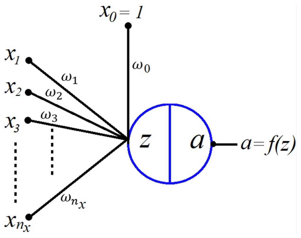
Figure 2.
Three steps of 2D convolution over a valid area of a kernel with one channel receptive field.
Figure 2.
Three steps of 2D convolution over a valid area of a kernel with one channel receptive field.
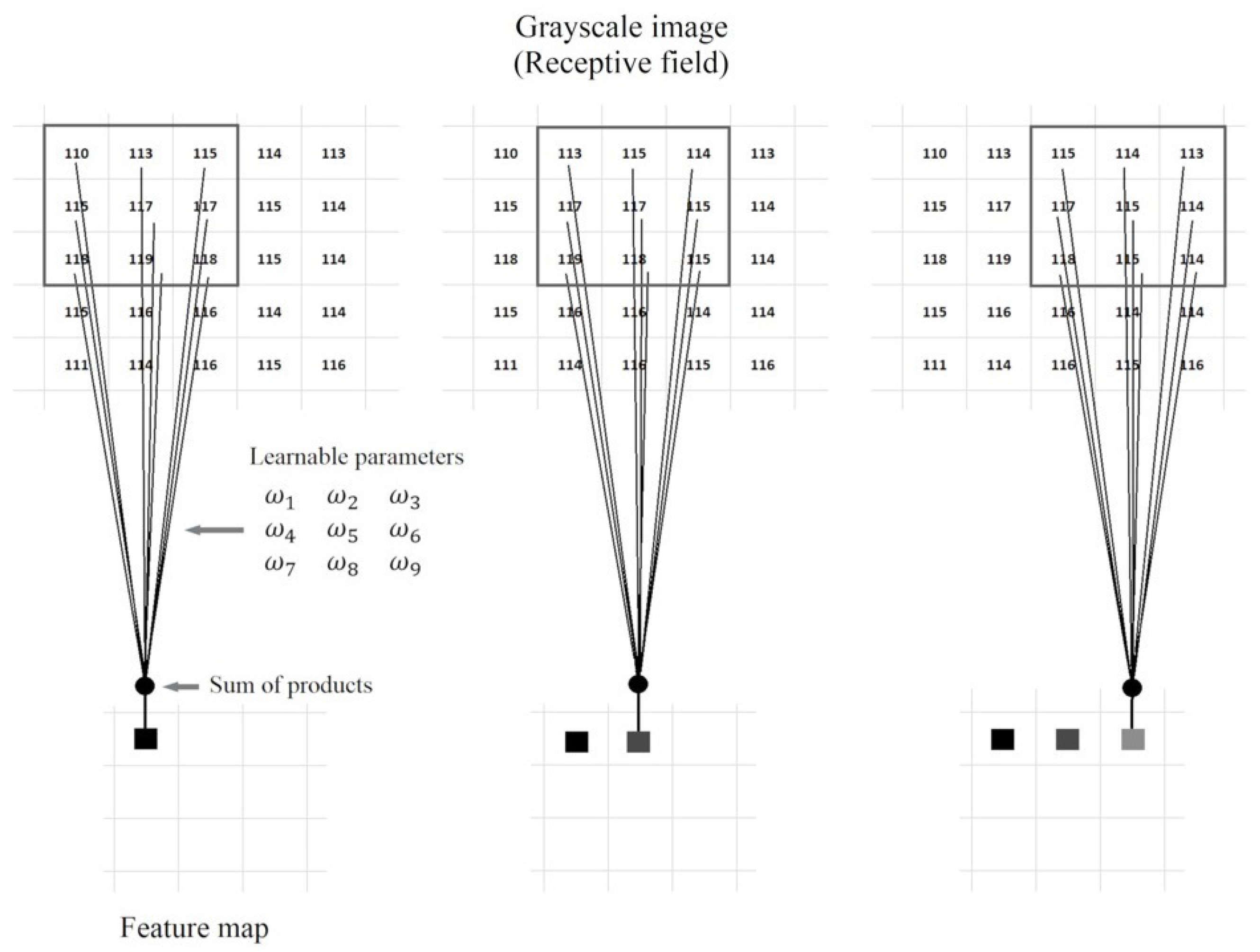
Figure 3.
One step of 2D convolution of a kernel with a three channels receptive field. The red, green, and blue squares represent the output of each filter, and the brown square is the final result or extracted feature. Notice that we need one filter per channel to produce one channel of features.
Figure 3.
One step of 2D convolution of a kernel with a three channels receptive field. The red, green, and blue squares represent the output of each filter, and the brown square is the final result or extracted feature. Notice that we need one filter per channel to produce one channel of features.
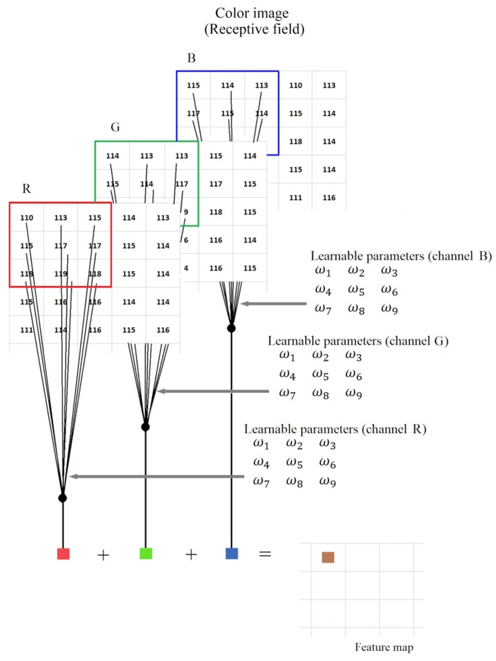
Figure 4.
2D filtering of 3D data over a valid area of the receptive field and their representation using volumes.
Figure 4.
2D filtering of 3D data over a valid area of the receptive field and their representation using volumes.
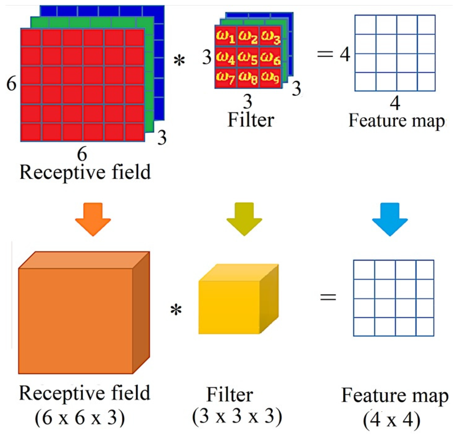
Figure 5.
The convolution of three 3D filters over a valid area of a 3D receptive field and the resulting feature maps represented by the green volume with three channels.
Figure 5.
The convolution of three 3D filters over a valid area of a 3D receptive field and the resulting feature maps represented by the green volume with three channels.
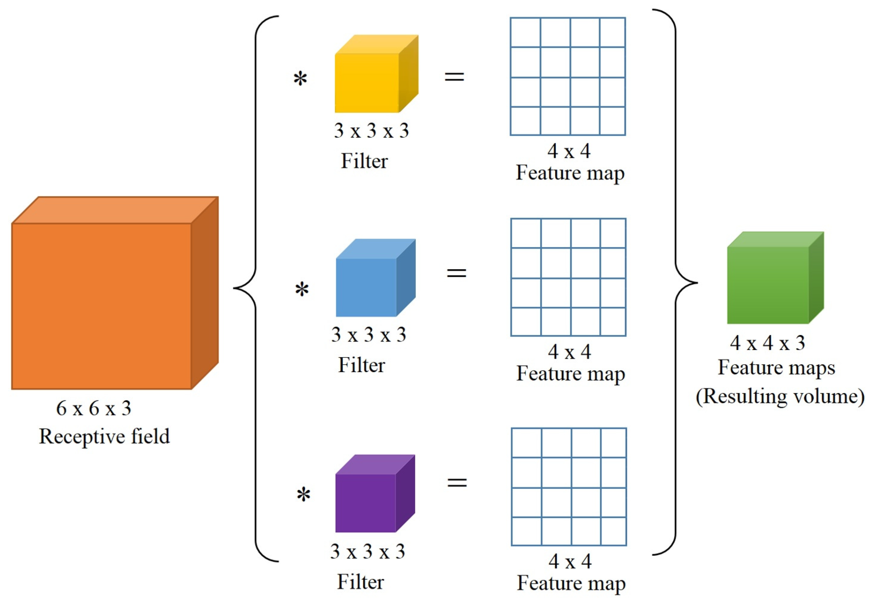
Figure 6.
Process for building one convolutional layer of size .
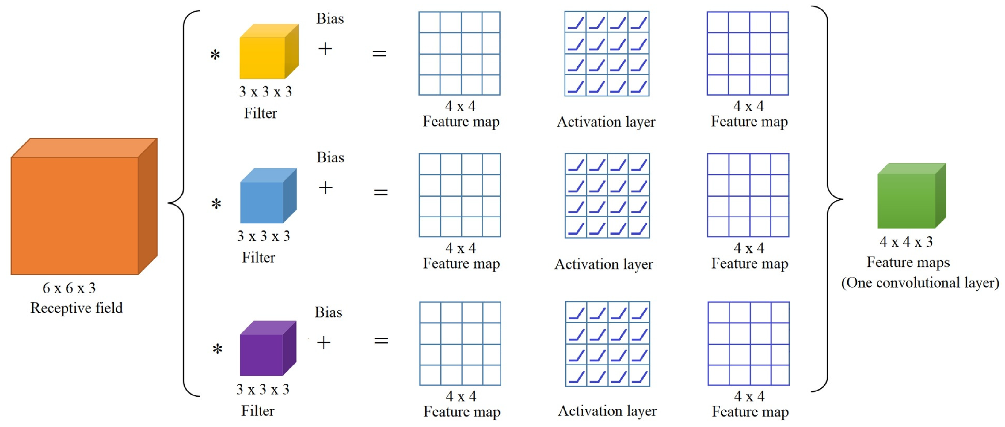
Figure 7.
Feature extraction to yield a 2D convolutional layer using a filter with zero padding of and stride in the receptive field.
Figure 7.
Feature extraction to yield a 2D convolutional layer using a filter with zero padding of and stride in the receptive field.
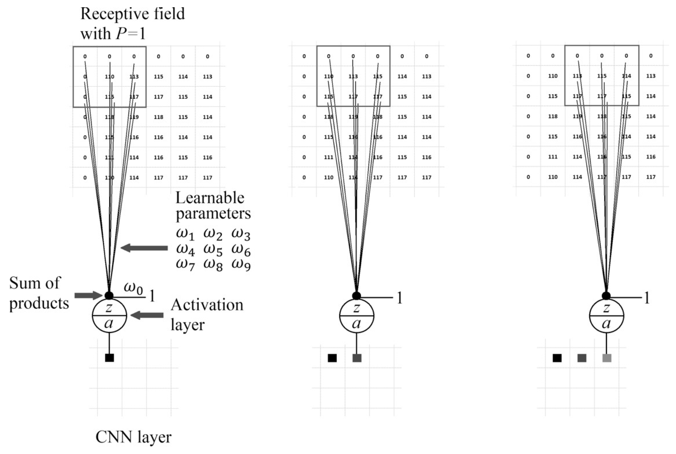
Figure 8.
Feature extraction to yield a 2D convolutional layer using a filter with zero padding of and stride in the receptive field.
Figure 8.
Feature extraction to yield a 2D convolutional layer using a filter with zero padding of and stride in the receptive field.
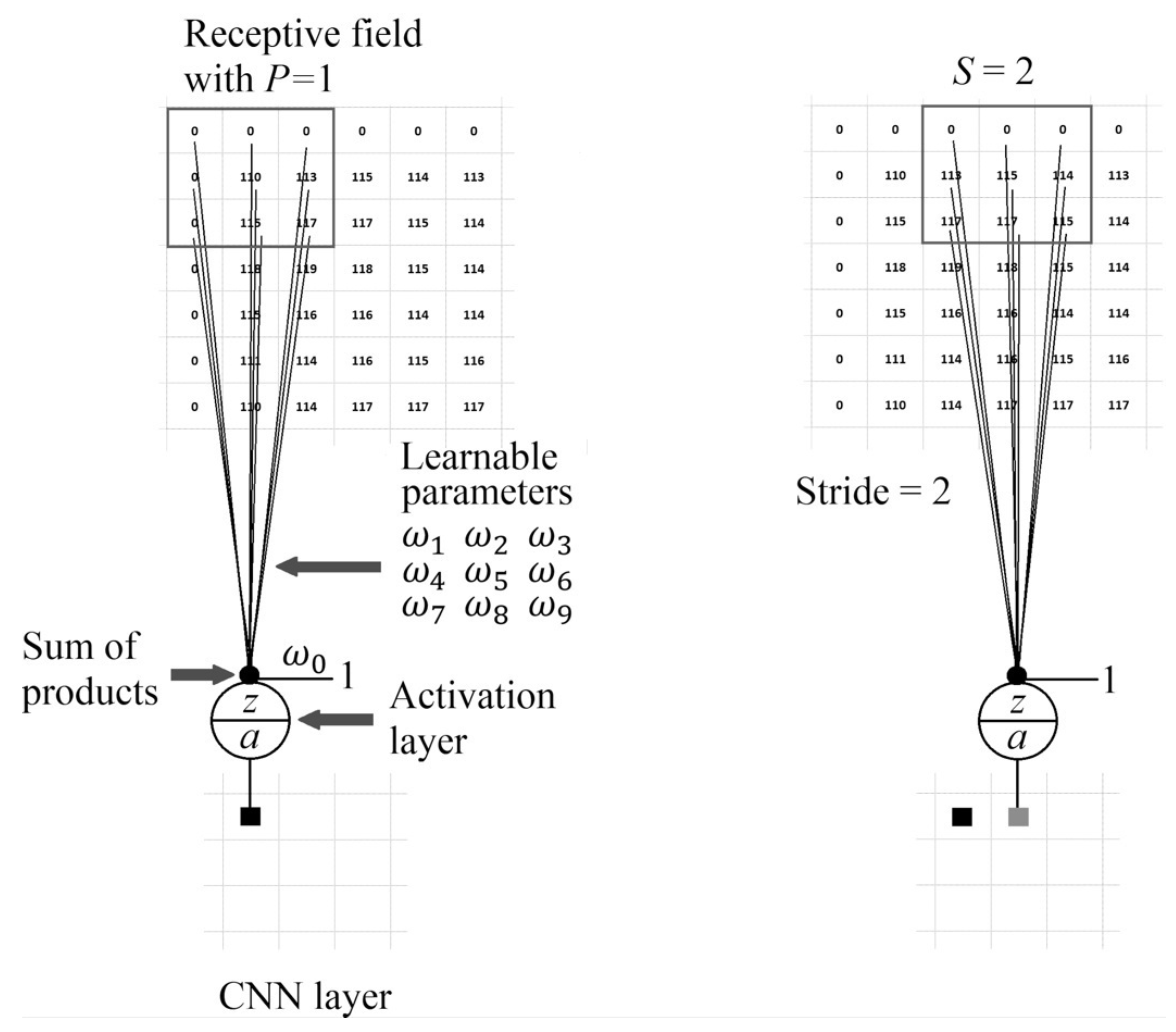
Figure 9.
One 2D convolutional layer obtained after filtering and the activation layer.
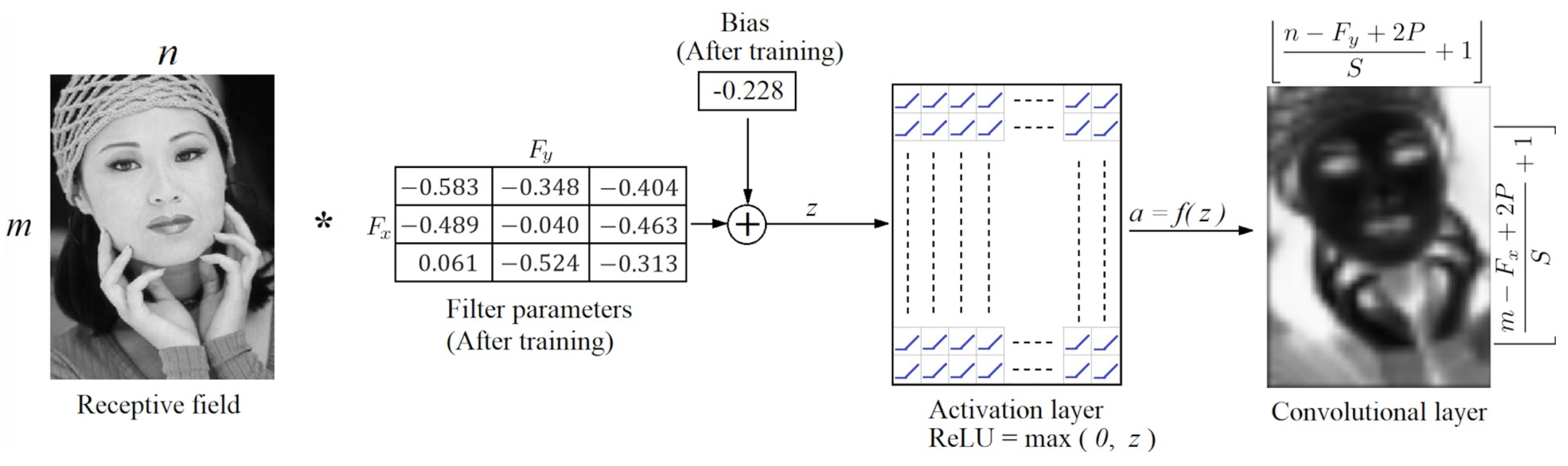
Figure 10.
One volumetric convolutional layer of size , obtained after convolving the receptive field with the learned parameters of 4 filters and the activation layers.
Figure 10.
One volumetric convolutional layer of size , obtained after convolving the receptive field with the learned parameters of 4 filters and the activation layers.
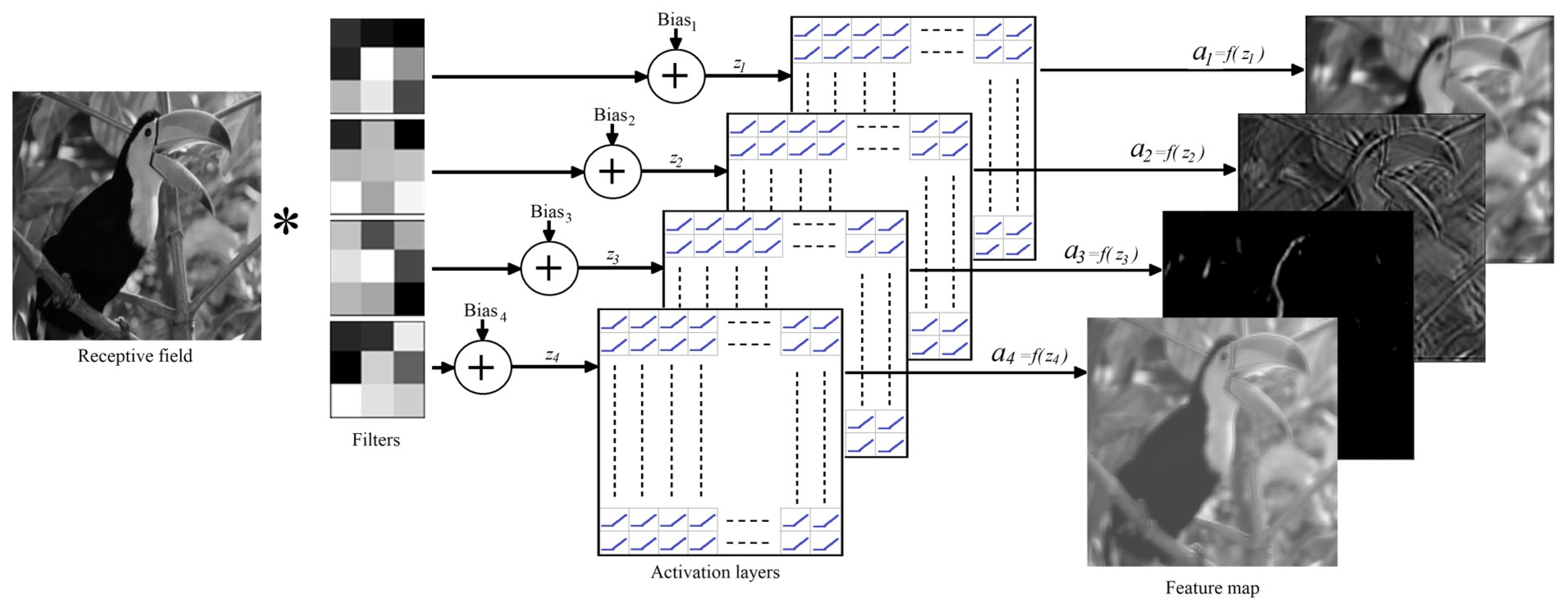
Figure 11.
3D Convolution and output features volume. The blue feature is yielded after the first convolution operation.
Figure 11.
3D Convolution and output features volume. The blue feature is yielded after the first convolution operation.
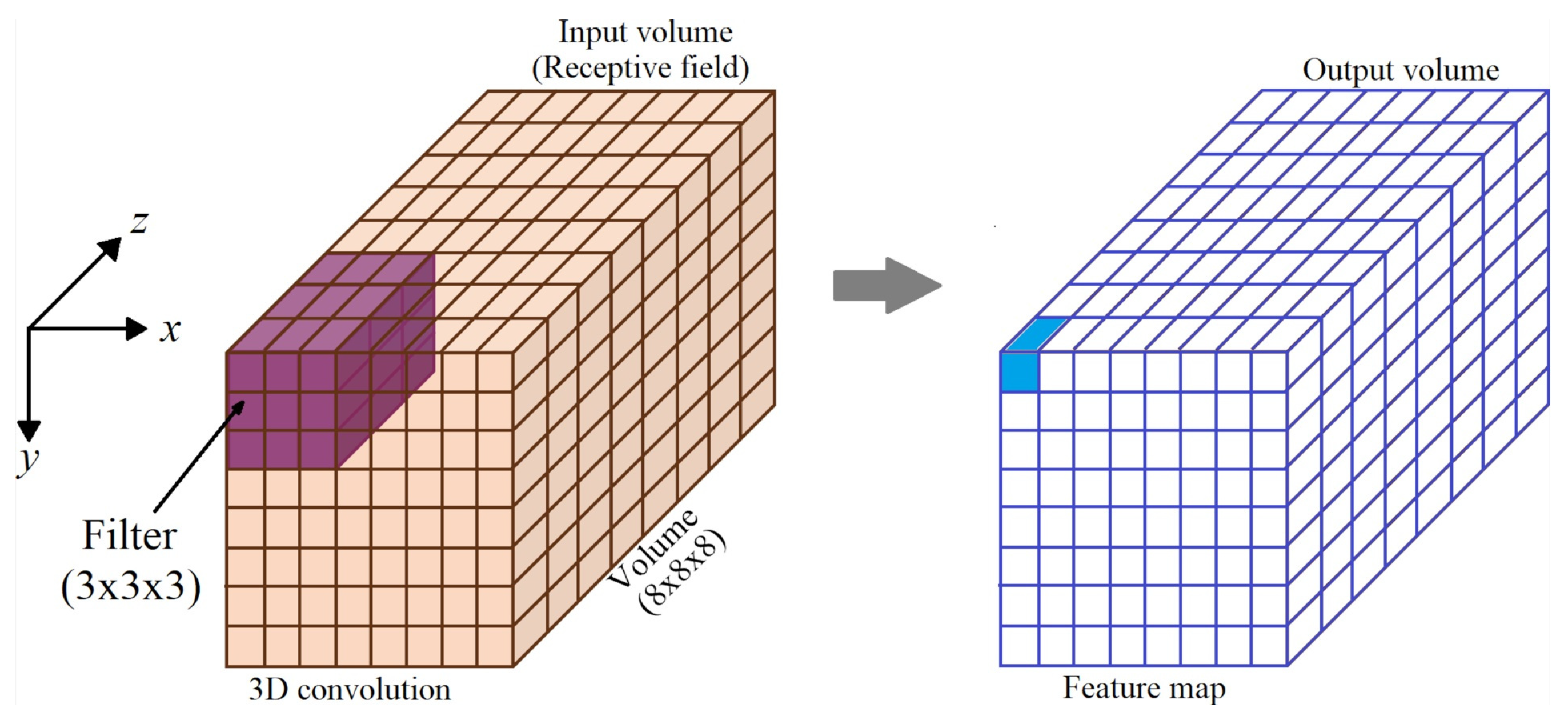
Figure 12.
1x1 convolution is used to reduce the dimension of a 3D receptive field to a 2D feature map. The blue squares are the output features that are yielded after 17 convolution operations. Notice that the depth of the filter is equal to the depth of the receptive field.
Figure 12.
1x1 convolution is used to reduce the dimension of a 3D receptive field to a 2D feature map. The blue squares are the output features that are yielded after 17 convolution operations. Notice that the depth of the filter is equal to the depth of the receptive field.
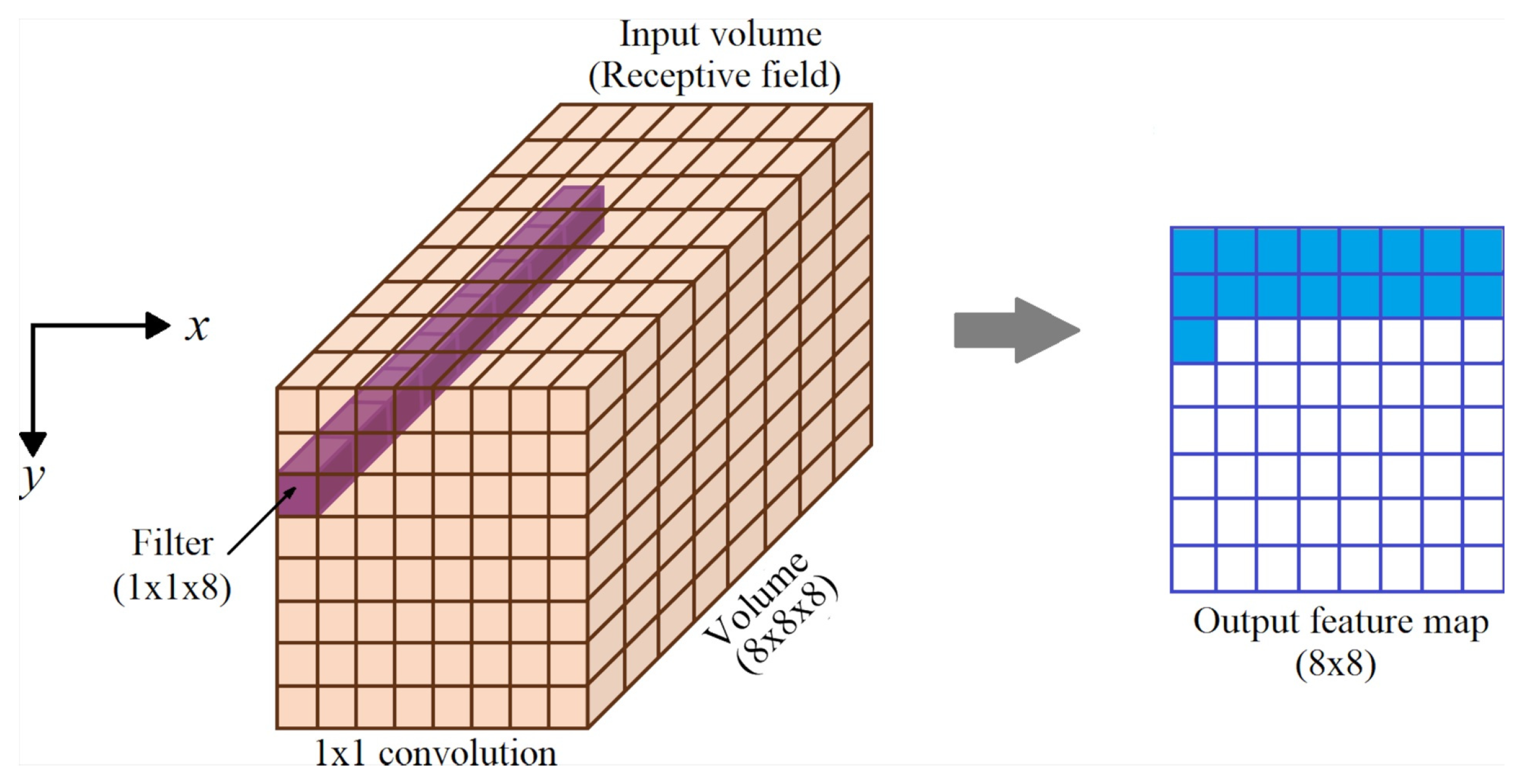
Figure 13.
Inception module with dimensionality reduction [23].
Figure 13.
Inception module with dimensionality reduction [23].
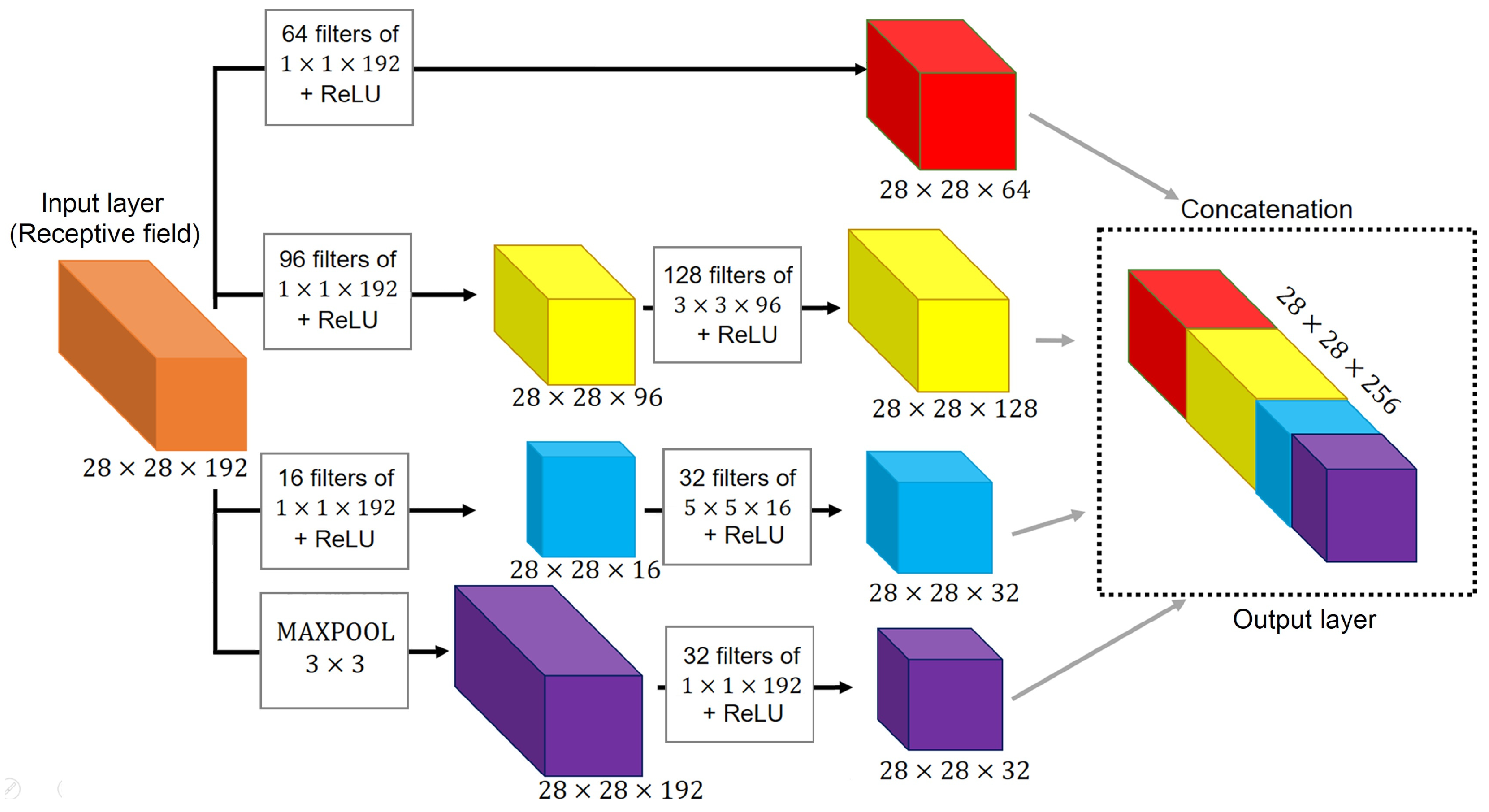
Figure 14.
Max pooling operation using a 2x2 window with no padding () and a stride ().
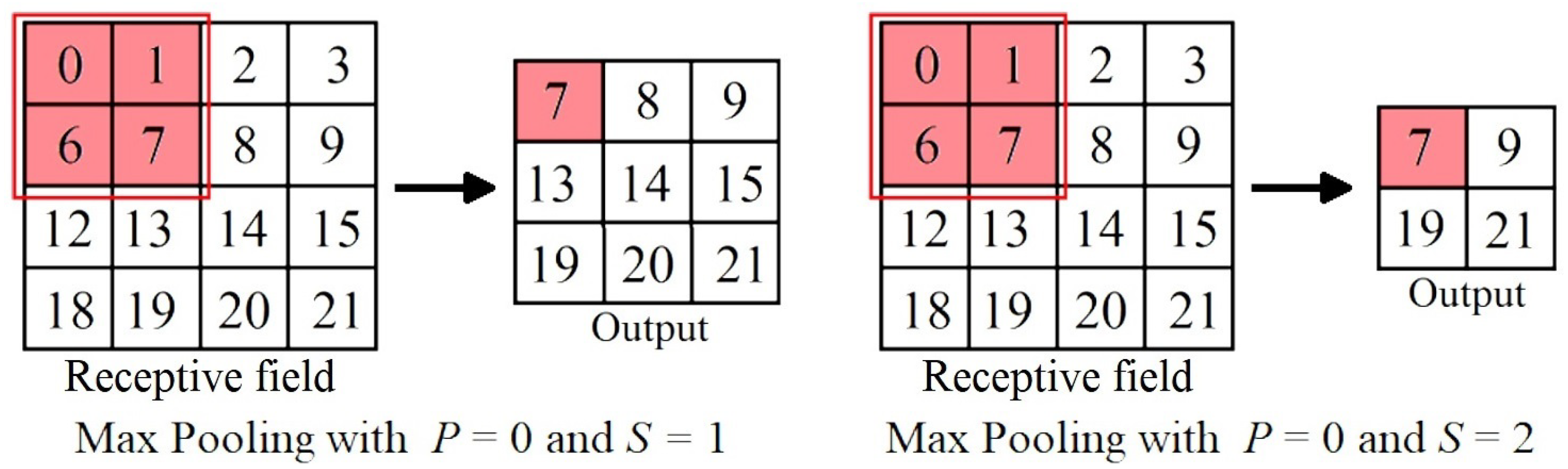
Figure 15.
Average pooling operation using a 2x2 window with no padding () and a stride ().
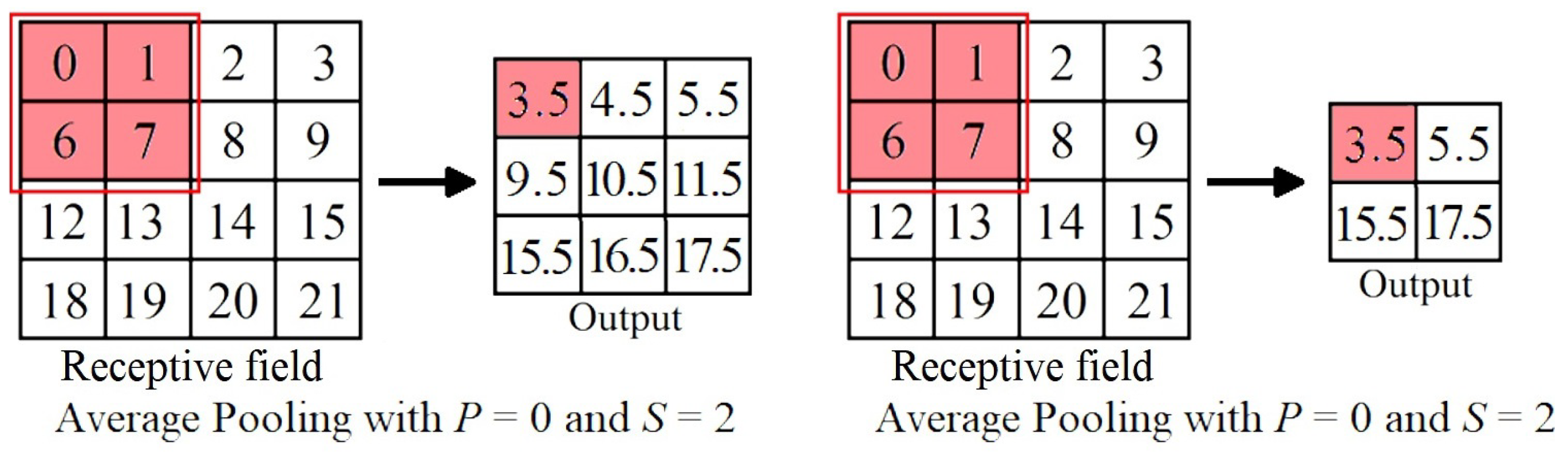
Figure 17.
Artificial neural network with four fully connected layers.
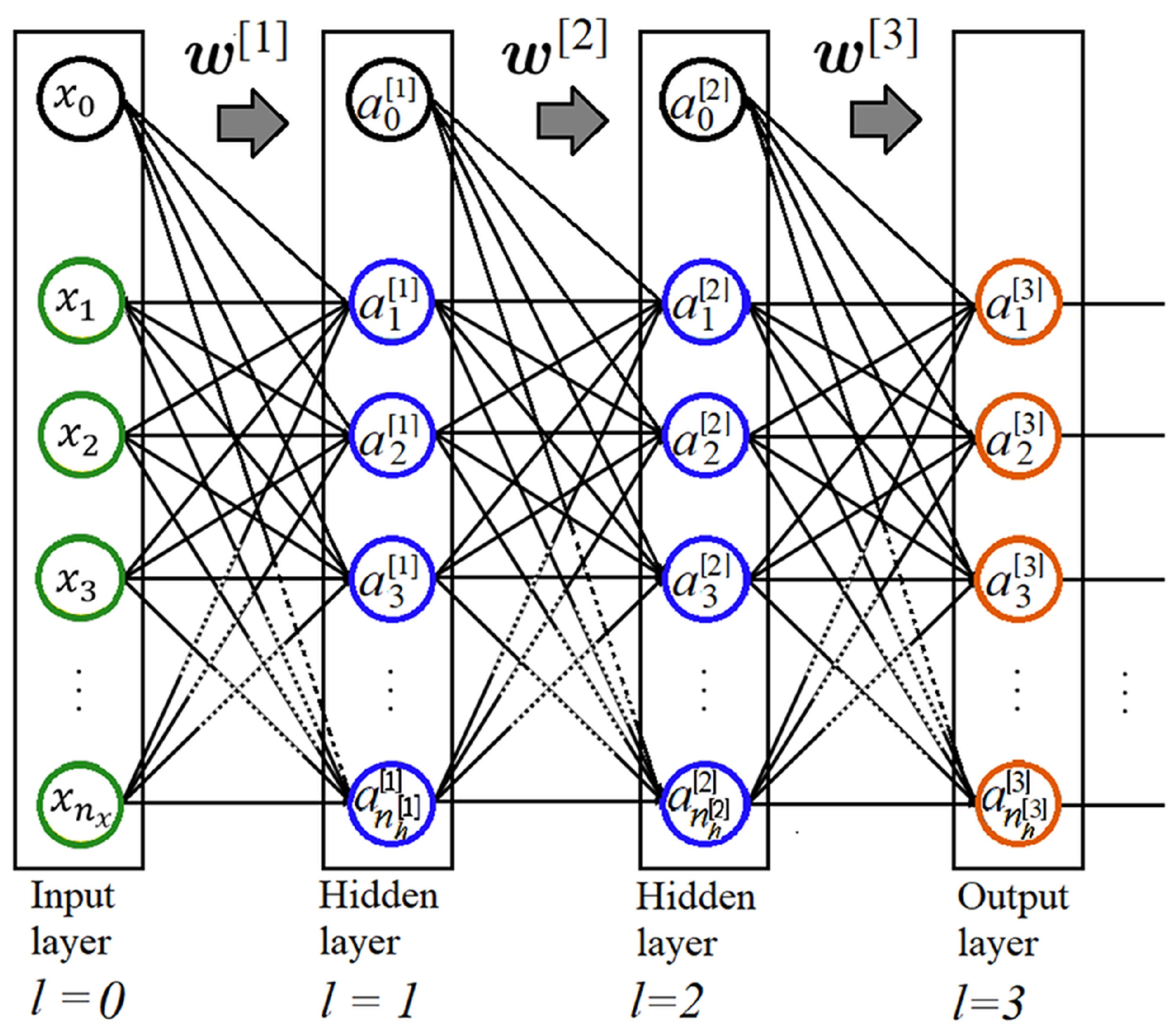
Figure 18.
Standard feed-forward DNN architecture with L dense layers.
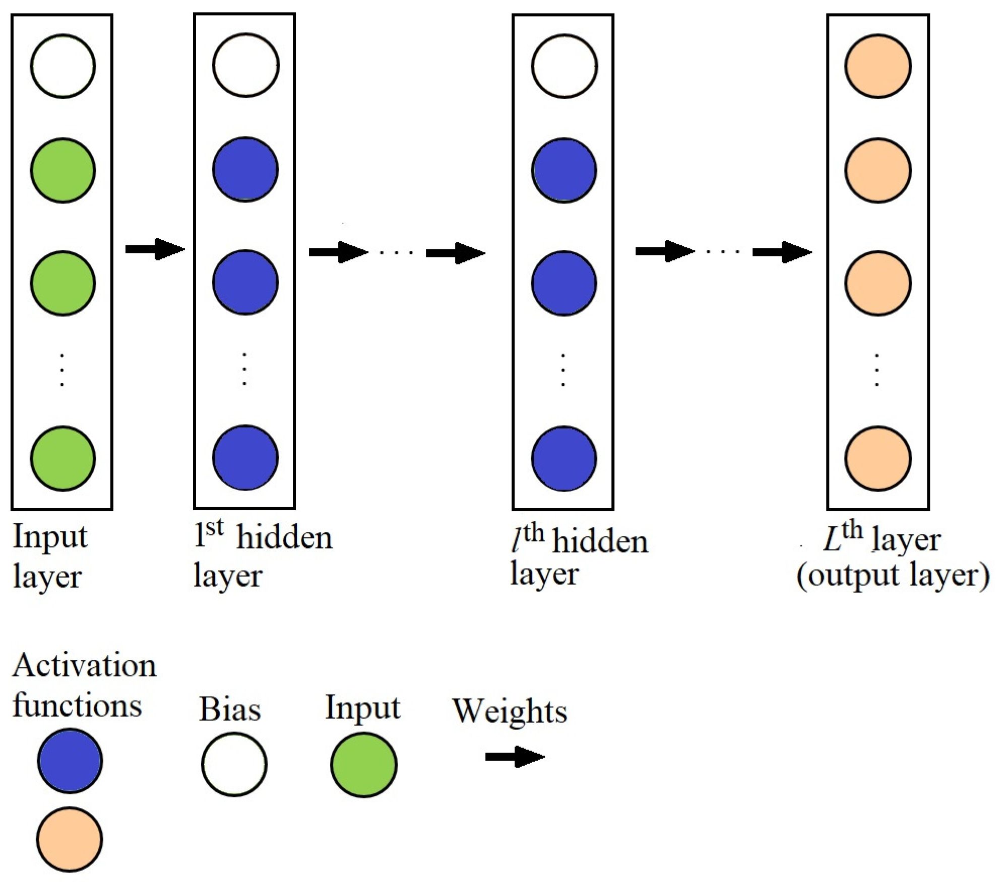
Figure 19.
Example of six tensors with different dimensions.
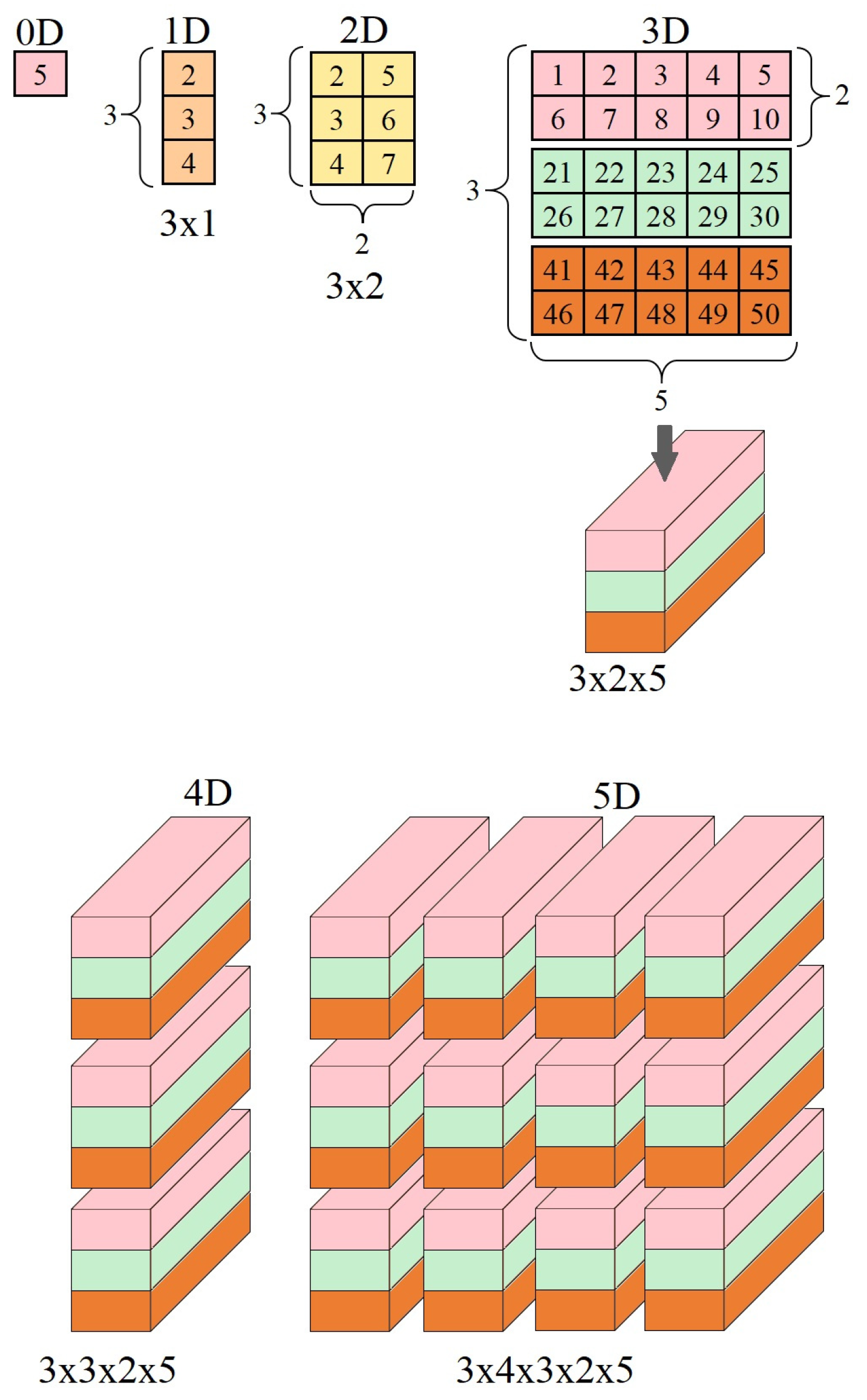

Table 1.
Some common activation functions.
| Name | Definition |
|---|---|
| Sigmoid | |
| Hyperbolic tangent | |
| Softmax | , |
| ReLU |
*K is the number of classes.
Disclaimer/Publisher’s Note: The statements, opinions and data contained in all publications are solely those of the individual author(s) and contributor(s) and not of MDPI and/or the editor(s). MDPI and/or the editor(s) disclaim responsibility for any injury to people or property resulting from any ideas, methods, instructions or products referred to in the content. |
© 2023 by the authors. Licensee MDPI, Basel, Switzerland. This article is an open access article distributed under the terms and conditions of the Creative Commons Attribution (CC BY) license (http://creativecommons.org/licenses/by/4.0/).
Copyright: This open access article is published under a Creative Commons CC BY 4.0 license, which permit the free download, distribution, and reuse, provided that the author and preprint are cited in any reuse.


