Deformable Riverbeds: A Numerical Study

1. Introduction

In most cases, the river channel position and depth change over time owing to channel deformation. Therefore, a forecast of channel deformations is required for the high-quality design of relevant structures and work performance. In addition, most rivers are regulated by the construction of reservoirs for energy and agricultural purposes. A large number of water-intake structures affect flow dynamics. The unique flow aspects of these rivers change the natural course of the riverbed process, and a forecast of riverbed change is required. Therefore, the study and development of the theory of channel processes and the dynamics of channel flows have always attracted the attention of researchers [1,2].

However, despite the abundant work devoted to forecasting channel deformations, its solution is still far from practical because of the complex and multifactorial nature of riverbed processes in space and time. In particular, great difficulties arise when designing various river structures, the bed of which, due to large bottom slopes, high flow velocities, and easy erosion of bottom sediments (represented by fine sandy soft soils), is subject to highly complex and intense deformations. An example of such a river in Uzbekistan is the Amu Darya.

The behavior of channel processes in easily eroded soils is very complex. Owing to the complexity and multifactorial causes that determine channel processes, as well as the lack of a rigorous theoretical solution to the problems of river hydraulics and the dynamics of channel flows, methods of physical and numerical modeling of channel processes are often used [3,4]. Both these methods complement each other, and as a result, it is possible to obtain more reliable solutions to the problem posed by the deformation of the channel in a specific section.

Numerical or physical modeling is used to solve the problem of channel processes, which can provide a specific forecast of channel deformations in the area of the structure. Despite such long practical experience, achieving an acceptable balance between the requirements of water transportation systems and the structures themselves, especially in meandering channels composed of easily eroded soils, is a complex and pressing engineering task [5,6].

A typical research object of channel processes is the Amu Darya River, which is easily eroded in the middle reaches. Numerical and physical methods are the most essential directions in channel-process research. However, significant problems with similar and distinctive features arise in both research directions.

The general problem is to find the fundamental physical laws and create a mathematical model (closed system of equations) to describe the process accurately. Based on this finding, the mathematical model can be both stochastic and deterministic. After drawing up such a model, the problems of the two modeling methods become entirely different.

Physical modeling is based on finding the conditions for connecting the model and nature by analyzing the system of equations under study [7,8,9]. This analysis was based on the following:

• The use of a similarity transformation would show that a process on a smaller scale (on a model) is equivalent to a process on a larger scale (in reality).
• finding modeling criteria based on it;
• establishing areas of self-similarity according to various criteria if they exist.

Ultimately, the rules for converting the model to the actual were obtained. Very often, a considerable model scale or expensive materials are required, which is associated with significant material costs.

Currently, hydraulics is experiencing a period of rapid development in numerical models. The numerical model represents a method of calculating the quantities necessary for practice, as described by the above system of equations. A numerical model can be either an exact or an approximate solution to a system of equations. In more or less complex cases, exact solutions are impossible. Therefore, it is necessary to use approximate numerical models. The most developed numerical models are based on discretizing temporal and spatial variables.

The main disadvantage of such models is the unknown degree of approximation of the solution to the original equations. It is almost impossible to prove strictly the convergence of a discrete problem to the original solution. It is necessary to demonstrate such convergence empirically by comparing it with the test problems. However, compared with physical modeling, numerical modeling requires less time and labor, allowing for more multivariate studies and considering more factors influencing the process. Therefore, numerical modeling of physical processes and numerical modeling of channel processes play an increasingly important role.

The fastest and most robust way to describe river flow or open channel flow is based on 1D Saint-Venant equations [10,11,12], also called shallow water equations. On the one hand, this approach has low computational cost and can provide results quickly. However, this method cannot capture complex flow with 3-dimensional inertial effects. The next logical step is the 2D shallow water equation, which can be significantly more accurate [13]. 2D models provide more accuracy through more computational cost, so hybrid methods also couple 1D and 2D approaches [14,15,16] to obtain more robustness than 1D methods and less computational cost than 2D methods.

Specific numerical codes have been designed to describe various river flows. For example, HEC-RAS 2D (Hydrologic Engineering Center's River Analysis System from U.S. Army Corps of Engineers)[17,18,19,20], LISFLOOD-FP[19] and SRH-2D [20] (developed by U.S. Bureau of Reclamation) The two turbulence models that SRH-2D suggests are the depth-averaged parabolic and k-epsilon models. Since the parabolic model is the only turbulence model utilized by Hydro_AS-2D and a proper comparison requires the same parameters, it is employed in this study. A wetting drying front limit of 0.001 m was used in the SRH-2D. The water depth on the cell is regarded as 0 m below this value, and SRH-2D is unable to solve shallow water equations. These codes are based on two-dimensional shallow water equations and employ finite-volume or finite-difference methods to solve them. This approach is known for its robustness and mass and momentum conservation (for F.V.M. methods only); however, it requires a digital elevation map (D.E.M.) as a boundary condition. The most common application of these software packages is to predict the consequences of floods.

When solving the conjugated model with bed deformation, the 2D model is preferable because it accurately predicts near-wall friction. Turbulence is considered to obtain even higher accuracy in terms of friction [21]. There are also several approaches for turbulence modeling in shallow water equations, all of which are similar to Navier-Stokes-based equations. Depth-averaged shallow water equations with turbulence models based on transport equations were based on the RANS approach. Large-scale turbulent structures can also be modeled directly, as they occur in the LES/DES family methods [22]. There were also modifications to the DA SWE method [23].

The studies [24,25] have revealed that the process of deformation, including the flattening of an underwater slope with a rectilinear generatrix directed along the flow velocity, can be effectively described by a one-dimensional diffusion equation governing the bottom elevation within a watercourse:

$$(1-\mathrm{p}){\displaystyle \frac{\partial {\mathrm{Z}}_{\mathrm{b}}}{\partial \mathrm{t}}}={\displaystyle \frac{\partial }{\partial y}}D{\displaystyle \frac{\partial Z_b}{\partial y}},$$

(1)

Where:

p is the soil porosity coefficient.

Z_b (t,y) is the bottom elevation.

- t denotes the signified time

y is the coordinate across the slope;(

D is the diffusion coefficient characterizing the specific transverse sediment flow rate.

Furthermore, studies [26] established the relationship for the diffusion coefficient D. Analytical solutions to the initial boundary value problem associated with Equation (1) were also obtained, specifically for the hypothetical case of deformation of an underwater slope with an initial profile in the form of a vertical step in a channel of unlimited width.

The work in [27] facilitated the derivation of analytical solutions for a slot of a finite width. Additionally, the performance of the model was rigorously verified against a substantial dataset of field observations, demonstrating its effectiveness in solving practical problems.

$$(1-\mathrm{p}){\displaystyle \frac{\partial {\mathrm{Z}}_{\mathrm{b}}}{\partial \mathrm{t}}}=-{\displaystyle \frac{\partial U{S}_{*}h}{\partial x}}-{\displaystyle \frac{\partial V{S}_{*}h}{\partial y}},$$

(2)

Where:

• U and V are the components of the depth-averaged water velocity vector along the x- and y-axes, respectively.
• h (x,y,t) is the flow depth
• S (x,y,t)* is the saturation turbidity, which denotes the vertical average volume concentration of the sediment in an equivalent uniform flow.

Equation (2) has been instrumental in predicting channel transformations by assuming that saturation turbidity or equilibrium sediment concentration primarily depends on local flow characteristics and is related to them, such as uniform flow conditions. Using Equation (2) in conjunction with the two-dimensional Saint-Venant equations yielded satisfactory results in predicting channel transformations for various scenarios [28,29].

Equation (2) presents the limitations for describing planned deformations in channels that feature bottom sections with relatively steep slopes. Such slopes include dredging slots, quarries, or steep banks at bends. In a straight channel with an underwater slope, where the generatrix aligns with the velocity vector (and both the velocity vector and flow depth remain constant along the longitudinal coordinate x), Equation (2) implies that Z_b=const. Consequently, Equation (2) does not account for a well-recognized phenomenon: the alteration of an underwater slope with a generatrix parallel to the flow velocity vector. Non-accounting arises from the assumption in Equation (2) of the collinearity of water velocity and solid-phase flow vectors, which is not valid in all cases.

Equation (2) was enhanced by introducing terms that enable the Equation to account for the effect of the noncollinearity of water velocity and solid-phase flow vectors [30,31]. The incorporation of the diffusion terms into Equation (2) is theoretically justified. The incorporation of the diffusion term led to the derivation of an expression for the diffusion coefficient of the bottom mark, represented as a spherical tensor, with proportionality to the longitudinal specific sediment flow rate in the direction of the velocity vector:

$$(1-\mathrm{p}){\displaystyle \frac{\partial {\mathrm{Z}}_{\mathrm{b}}}{\partial \mathrm{t}}}+{\displaystyle \frac{\partial U{S}_{*}h}{\partial x}}+{\displaystyle \frac{\partial V{S}_{*}h}{\partial y}}={\displaystyle \frac{\partial }{\partial x}}D{\displaystyle \frac{\partial Z_b}{\partial x}}+{\displaystyle \frac{\partial }{\partial y}}D{\displaystyle \frac{\partial Z_b}{\partial y}}$$

(3)

Where $D=ahS{}_{*}\left|\overrightarrow{U}\right|$, $\left|\overrightarrow{U}\right|=\sqrt{U^2+V^2}$, and $\alpha$ is proportionality factor.

An alternative model was introduced in [32,33], which diverges notably from the prior model. The key distinction lies in the formulation of the diffusion term exclusively in the direction orthogonal to the flow velocity vector. Additionally, an extra term was incorporated to consider the impact of streamline curvature on alterations in bottom elevations. The diffusion coefficient is proportional not to the flow velocity but to the value of the non-shearing flow velocity. Applying this alternative model yielded remarkable results in predicting channel reformations. The previously mentioned deformation models [32,33] all operate assuming that the sediment particle concentration in the flow closely approximates equilibrium conditions. In [10], it was established that the specific sediment flow from the bottom to the flow thickness is proportional to the value ($S-S_{*}$).

This study aims to amalgamate the strengths of various previously mentioned models and propose a mathematical model for sediment transport in dynamic river flows. It is recommended to conduct numerical simulations of river flows characterized by deformable bottoms, as proposed in [8], to employ a mathematical model governed by a system of two-dimensional Saint-Venant equations [21] incorporating partial derivatives and closing relations.

Simulations of the hydrodynamic and dynamic changes in the relief of the riverbed were carried out, and models for the accurate calculation of changes in the layer level and area of deposition and erosion were proposed [34,35,36,37]. In [38,39,40], a hydraulic experiment was conducted to study the hydraulic phenomena of a dam by comparing hydraulic surges and flow characteristics. Although the sluice gates generated hydraulic surges similar to those in stationary dams, their supercritical flow increased downstream, which ultimately lengthened the overall hydraulic surge.

This study addresses the research gap in developing a comprehensive mathematical model that accurately predicts the behavior of mobile riverbed deformation, encompassing all pertinent effects. Previous models have either been overly simplistic or focused on specific aspects of riverbed deformation without considering the broader context.

This study aims to develop a comprehensive mathematical model that can accurately predict the behavior of mobile riverbed deformation, encompassing all pertinent effects. The model can describe deformations in uneven and unsteady river flows, including the movement of the dredging slots and channel quarries.

Based on the analysis above, the numerical research method was identified as the primary research method for this study. According to the purpose of the study, the main objectives of the study are outlined in the following interpretation:

• selection of the elementary flow equation;
• conducted numerical studies on the reformation of inclined channel walls with a moving bottom.
• conducting experimental studies
• comparison of the obtained results with the results of experimental studies.

2. Methods

2.1. Analytical studies

The analytical approach employed in this work involves:

• Choice of Flow Equation: The selection of the Equation governing flow movement in the riverbed is represented by a system of two-phase hydrodynamic equations of Saint-Venant. These equations were complemented by including equations related to sediment balance, transport, and the Bagnold Equation.
• Numerical and Experimental Studies: Numerical and experimental studies were conducted under the conditions of a moving bottom by utilizing the chosen equations.
• Comparison of Results: The results obtained from both the numerical and experimental studies were thoroughly compared and analyzed.

This analytical approach aims to comprehensively understand and model the dynamics of riverbed processes and deformations.

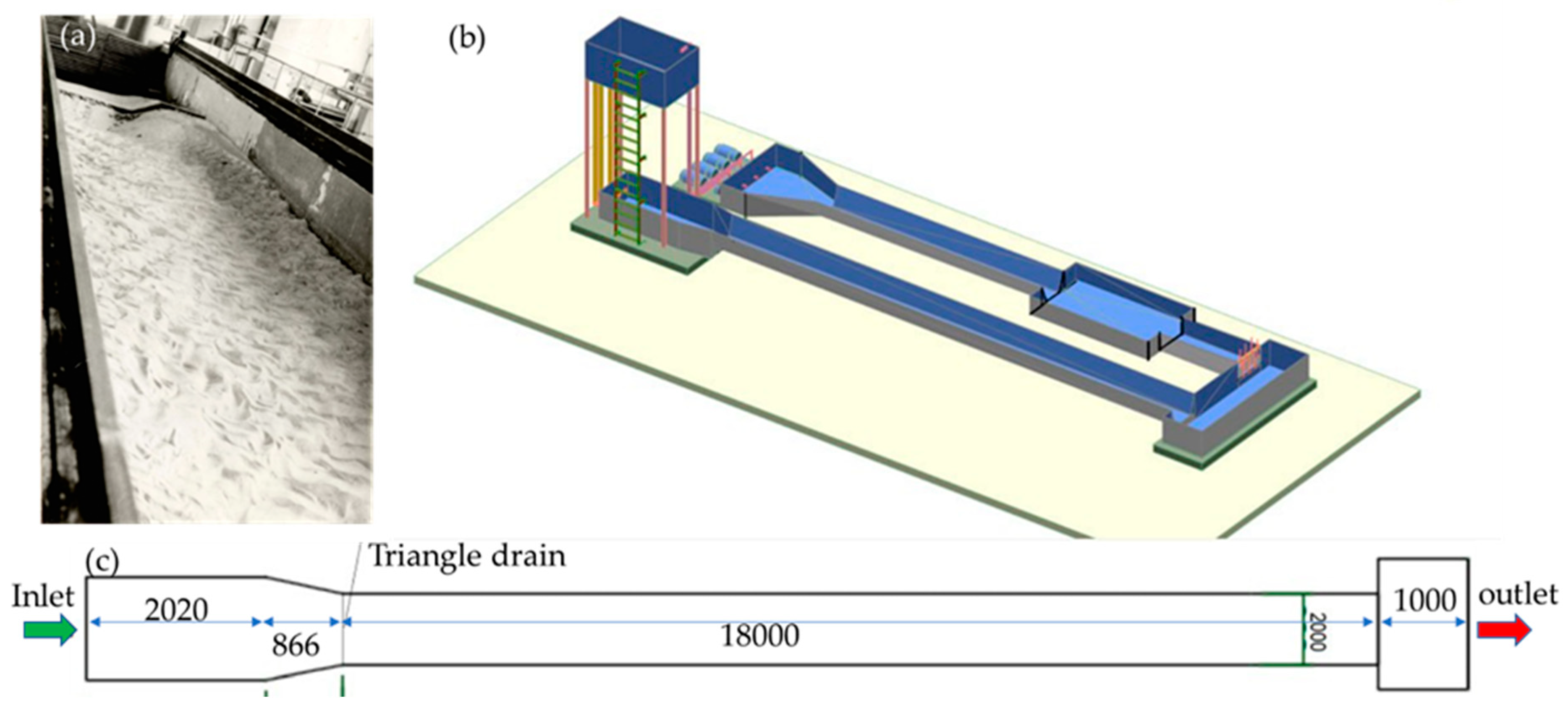
2.1. Experimental studies

Laboratory experiments were conducted to validate the model. The experiments focused on slope erosion by a current, where the current velocity vector aligns with the slope's generatrix. These experiments were conducted at the Hydraulics Laboratory of the Moscow State University of Civil Engineering, Moscow, Russia. The experimental setup and procedures were consistent with those previously documented in references [37,38,39].

The laboratory experiments were conducted within a channel featuring variable slope dimensions, with the following primary specifications: length of 18 m, width of 2 m, and wall height of 0.8 meters. The channel capacity allowed for a flow rate of up to 4 cubic meters per second, and the slope ranged from 0 to 0.1. Water flow measurements were performed using a triangular weir positioned at the outlet of the channel. A specialized pocket was integrated at the end of the working section of the flume to collect sediment and accommodate the experiments. A swinging shield was employed during the experiments to regulate the flow level of the channel. The longitudinal slope was maintained at 0.0027 during the experiment.

Figure 1 illustrates the eroded model. Table 1 shows the granulometric composition of sand. Specifically, sand had a mean diameter of 0.24 millimeters.

The cross-sectional shape of the model closely resembled half of the cross-section of a trapezoidal channel with a slope coefficient of m=2. Before commencing water flow, a thorough horizontal survey of the bottom was conducted. Water was incrementally introduced into the flume simultaneously from the upper and lower tails to ensure minimal disturbances to the bottom before the start of each experiment. Throughout the experiments, measurements were taken at defined intervals to record the bottom surface and free surface of the water in fixed sections. These measurements were then averaged to obtain comprehensive data for analysis.

3. Results

3.1. Mathematical model

As recommended in [8], a mathematical model based on a system of two-dimensional Saint-Venant equations [10] incorporating partial derivatives and closing relations to perform numerical calculations of river flows characterized by deformable bottoms was employed. This mathematical model serves as a foundational framework for understanding and predicting the complex dynamics of river flow.

$${\displaystyle \frac{\partial hS}{\partial t}}+{\displaystyle \frac{\partial USh}{\partial x}}+{\displaystyle \frac{\partial VSh}{\partial y}}=-K(S-S_{*})$$

(4)

$$(1-\mathrm{p}){\displaystyle \frac{\partial {\mathrm{Z}}_{\mathrm{b}}}{\partial \mathrm{t}}}=K(S-S_{*})+{\displaystyle \frac{\partial }{\partial x}}D{\displaystyle \frac{\partial Z_b}{\partial x}}+{\displaystyle \frac{\partial }{\partial y}}D{\displaystyle \frac{\partial Z_b}{\partial y}}$$

(5)

$$K=\left\{\begin{array}{c}\alpha U_{*}+(1-\alpha )W,U_{*}\ge W\\ W,U_{*}\le W\end{array}\right.;0\le \alpha <1$$

(6)

$$D=\beta \tilde{S}hW$$

(7)

$$S_{*}={\alpha }_1{\displaystyle \frac{\lambda \rho }{2{\rho }_s}}{\displaystyle \frac{{(\left|\overrightarrow{U}\right|-U_N)}^2}{gh}}\left({\displaystyle \frac{0.13}{tg\varphi }}+0.01{\displaystyle \frac{\left|\overrightarrow{U}\right|}{W}}\right),\lambda =2g{n}^2{h}^{-1/3}$$

(8)

where

• $t$ is the time; $h$ is the flow depth;
• U and V are the components of the flow velocity along the X and Y axis, respectively.
• $\left|\overrightarrow{U}\right|=\sqrt{U^2+V^2}$;
• $S$ is the volumetric concentration of sediment particles in the flow;
• $S_{\mathrm{*}}$ Is the equilibrium volume concentration of particles (saturation concentration) calculated according to the modified Bagnold formula:
• $K$ is the intensity coefficient of vertical sediment exchange between the bottom and the stream, $p$ is the soil porosity (the ratio of the volume of pores to the volume of the entire soil with pores).
• ${\rho }_s,\rho$ is the densities of soil and water, respectively;
• φ is the angle of internal friction of the soil.
• $W$ is the hydraulic soil coarseness;
• $U_{\mathrm{*}}$ Is the dynamic speed;
• $\left|\overrightarrow{U}\right|$, $U_N$ These are the modules of the average vertical flow velocity and non-shear velocity, respectively.
• $\lambda$ is the coefficient of hydraulic friction calculated using the Manning formula, $n$ is the roughness coefficient.

The Saint-Venant equations [10] are as follows:

$$\left\{\begin{array}{c}{\displaystyle \frac{\partial \left(\rho h\right)}{\partial t}}+{\displaystyle \frac{\partial \left(\rho h{v}_i\right)}{\partial x_i}}=0\\ {\displaystyle \frac{\partial \left(\rho h{v}_i\right)}{\partial t}}+{\displaystyle \frac{\partial \left(\rho h{v}_i{v}_j\right)}{\partial x_j}}={\displaystyle \frac{\partial }{\partial x_j}}\left({\displaystyle \frac{\mu }{\rho }}h{\displaystyle \frac{\partial v_i}{\partial x_j}}+h{\displaystyle \frac{{\tau }_{ij}}{\rho }}\right)-gh\left({\displaystyle \frac{\partial h}{\partial x_i}}+{\displaystyle \frac{\partial Z_b}{\partial x_i}}\right)-{\displaystyle \frac{{\tau }_i^b}{\rho }}\end{array}\right.$$

(9)

where $v_i=\left[U,V\right],v_j=\left[V,U\right],x_i=\left[X,Y\right],x_j=\left[Y,X\right],$ ${\tau }_{ij}$ is the depth-averaged effective stress; $\mu$ is the viscosity; Zb is the bed elevation; ${\tau }_i^b$ These are the two components of the bed friction stress from the Manning formula.

To determine the non-shear velocity in the calculations, the formula provided by representatives of channel hydraulics is utilized, which, considering standard coefficient values, is expressed in two formally equivalent forms:

$$U_N=\lg {\displaystyle \frac{8.8h}{d_{90}}}\sqrt{{\displaystyle \frac{2}{3.5}}\left[({\rho }_s-\rho )g{d}_{50}+1.25C_y^H\right]}$$

(10)

$$U_N=0.18\sqrt{{\displaystyle \frac{2}{3.5\lambda }}\left[({\rho }_s-\rho )g{d}_{50}+1.25C_y^H\right]}$$

(11)

where $C_y^H$ is soil adhesion in t/m², $d_{50}$ is the average diameter of soil particles, $d_{90}$ is 90% of the soil particle diameter.

In the calculations of the diffusion coefficient (Equation 7), three variants of the formulas for $\tilde{S}$ are employed:

a) Based on the total equilibrium concentration of transportable and suspended sediments:

$$\tilde{S}=S_{*}$$

(12)

b) Derived from bottom equilibrium concentration:

$$\tilde{S}={\alpha }_1{\displaystyle \frac{\lambda \rho }{2{\rho }_s}}{\displaystyle \frac{{(\left|\overrightarrow{U}\right|-U_N)}^2\cdot 0.13}{ghtg\varphi }}$$

(13)

c) Utilizing bottom concentration "without square."

$$\tilde{S}={\alpha }_1{\displaystyle \frac{\lambda \rho }{2{\rho }_s}}{\displaystyle \frac{(\left|\overrightarrow{U}\right|-U_N)\left|\overrightarrow{U}\right|\cdot 0.13}{ghtg\varphi }}$$

(14)

The initial conditions are defined for the initial bottom surface $Z(x,y,0)$, the corresponding instantaneous fields of velocity. $\overrightarrow{U}(x,y,0)$, depth h(x,y,0), and concentration S (x,y,0).

The boundary conditions for (9-13) are as follows:

–

On solid boundaries, the condition of no flow is specified.

–

For liquid boundaries, flow rates or water levels are typically specified.

–

Water flowed into the computational domain through the boundaries of the computational domain, and the precipitation concentration was set at these boundaries.

–

Complex boundary conditions are also occasionally used. Complex boundary conditions can link costs with levels and non-reflective boundary conditions.

The solution for equations (4) and (5) concerning sediment concentration and bottom marks was obtained using the finite volume method on mixed triangular-quadrangular grids combined with the Saint-Venant equations.

The developed numerical scheme aligns with the scheme for the continuity equation of the liquid phase, which helps prevent the occurrence of the so-called dipoles as sources and sinks of mass. It utilizes a directed difference-type scheme to eliminate unphysical oscillations in the bottom topography, maintain transportability, and implement a difference analog of mass conservation for the solid phase.

Equations (4) and (5) represent a minimal approach for modeling the processes of bottom deformation in uneven and non-stationary river flows. Disregarding Equation (4) implies that the concentration in the flow is close to equilibrium and does not permit the specification of boundary conditions for the concentrations. Eliminating terms from Equation (5), which describes the diffusion of bottom marks, makes it impossible to account for the processes of transformation (flattening) of underwater slopes. Moreover, to describe three distinct physical processes (uplift-sedimentation, longitudinal sediment transport, and transverse diffusion of bottom marks), at least three empirical coefficients are required. In this model, the empirical coefficients were α, β, α₁. The choice of closing relations for models (6)–(13) remains an open question and requires further research.

Calculations for identical conditions were conducted, assuming a value of 0.5 for the test problems. The types of closing relations (7)–(13) and parameters were varied during the calculation process.

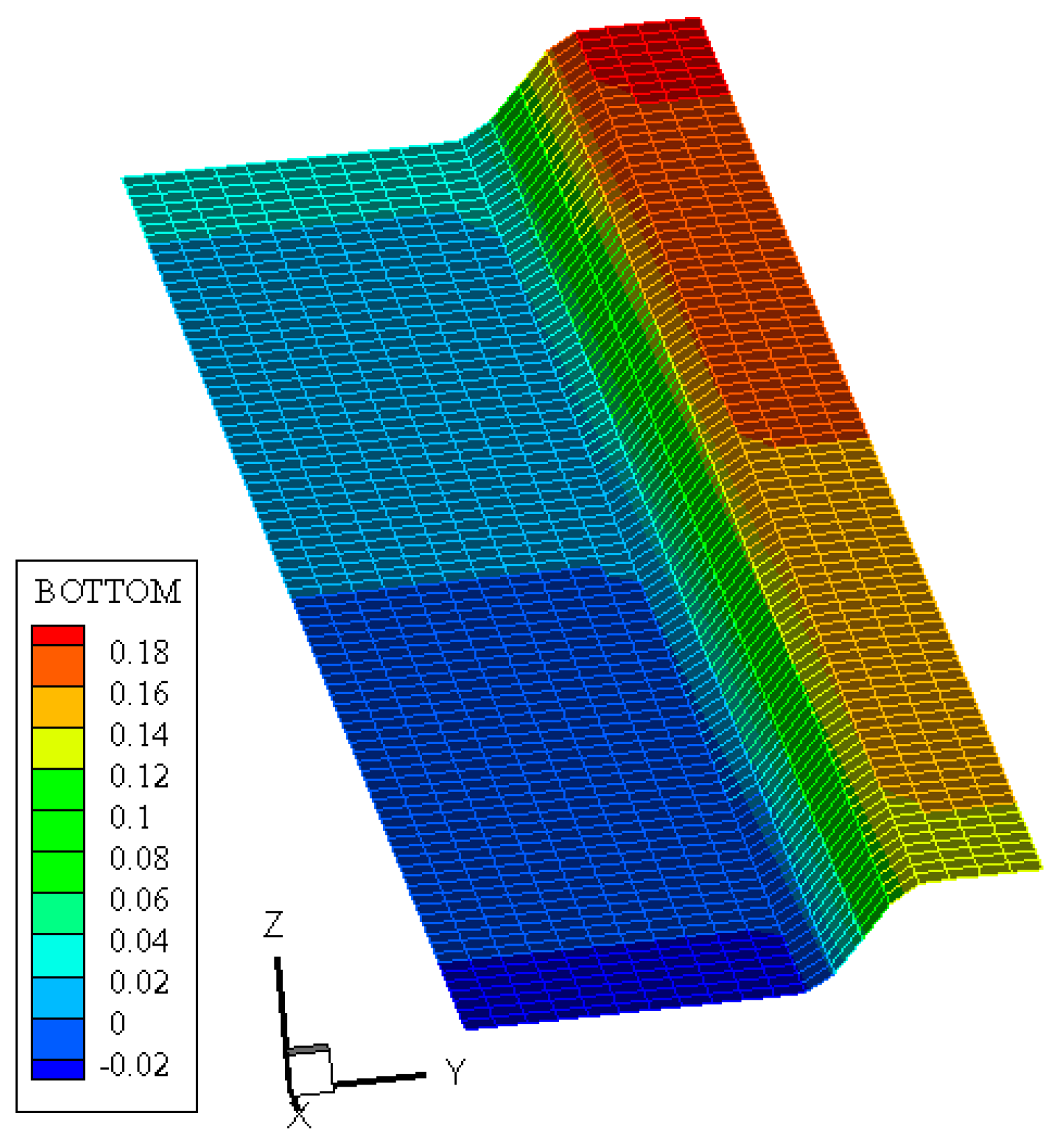
3.2. Numerical model

The calculations were conducted using Equations (4) and (5): A rectangular grid consisting of 1800 cells measuring 0.1 m × 0.2 m was constructed for a tray with 18.0 m × 2.0 m dimensions. At the entrance boundary corresponding to the first row of cells, it was assumed that the bottom was not eroded, which matched the entrance section of the tray reinforced with cement crust in the laboratory experiment. "Figure 2 illustrates the bottom marks and the rectangular grid employed in the numerical model of an eroded slope."

In the first step, the water flow rate at the inlet boundary was set to Q = 112 l/s, and the flow was set as specified (S = 0). The parameters of the numerical model, α_1 and β, were selected during the calculation process to achieve the best agreement in the average diameter of the flume between the calculated profile of the eroded slope and the experimental data. The calculation results are presented in Figure 3, Figure 4 and Figure 5.

Figure 3, Figure 4 and Figure 5 illustrate the different scenarios and parameters used in the calculations and their impacts on the flattening or leveling of the slope. The results demonstrated the importance of selecting appropriate parameters to achieve the best agreement with the experimental data.

The interaction between the flow and the moving bottom in the quarry zone, which typically occupies only a part of the river's width, has been studied in detail. In actual conditions, the interaction between the flow and the moving bottom in the quarry area is spatial, making the physical picture of the processes more complex and not fully describable in a one-dimensional setting.

The results of model studies conducted at the State Hydrological Institute, Moscow, Russia, in a hydraulic tray (2.0 m × 50.0 m) with a moving bottom were utilized to test the models. The bottom slope of the tray was 0.00125. The flow rate at the flume inlet was set to Q = 40 l/s. During the establishment of the flow, a stable ridge relief was formed, which acquired a three-dimensional structure and a scaly character. The average water depth increased from 6.65 cm to 8.86 cm, and the average flow speed decreased from 30.1 cm/s to 22.5 cm/s.

After achieving a quasi-uniform regime in the hydraulic flume, a riverbed quarry with a width of 0.7 m, which occupied 35% of the flume width, was mined. The quarry was initially located in the axial part of the tray at a depth of approximately 14 cm. The thickness of the sand layer at the bottom of the quarry is 3.0 cm. The sediment supply at the entrance boundary was 1.82 l/h (S = 0.02 kg/m³), with an average diameter of the initial soil being 0.32 mm.

The experiment in [8] described the process of bottom transformation, with background erosion deformations developing in the areas above and below the quarry. Above the quarry, erosion began in the axial part of the flow, whereas below the quarry, erosion occurred more intensively. The highest bottom marks are observed in the edge areas near the upper ledge, which moved downstream.

For the numerical simulation of these experimental studies, a rectangular grid of 5250 cells was constructed, and the roughness coefficient was set to 0.027 to match the steady-state depths and fluid velocities to the experimental data without a quarry. The calculations were then performed in the presence of a quarry. The diffusion coefficient was determined from the bottom concentration (12) and non-shear velocity using Equation (9) with β = 15 and α_1 = 1.0. A comparison of the results between the calculations and experiments showed almost complete qualitative and quantitative agreement.

This extensive analysis and comparison demonstrates the model's ability to accurately represent and predict the behavior of flow and bottom interactions in complex real-world scenarios.

4. Conclusions

This study developed a comprehensive mathematical model to depict riverbed deformation behavior accurately. The conclusions of this study can be summarized as follows.

• The proposed mathematical model (Section 3.1) and numerical model (Section 3.2) for bottom deformations in uneven and unsteady river flows are suitable for calculating deformable channels, making them applicable to scenarios such as easily eroded beds. The models are characterized by their simplicity, with a minimum number of equations and empirical constants.
• Two-dimensional mathematical and numerical models of a deformable channel were developed and successfully verified.
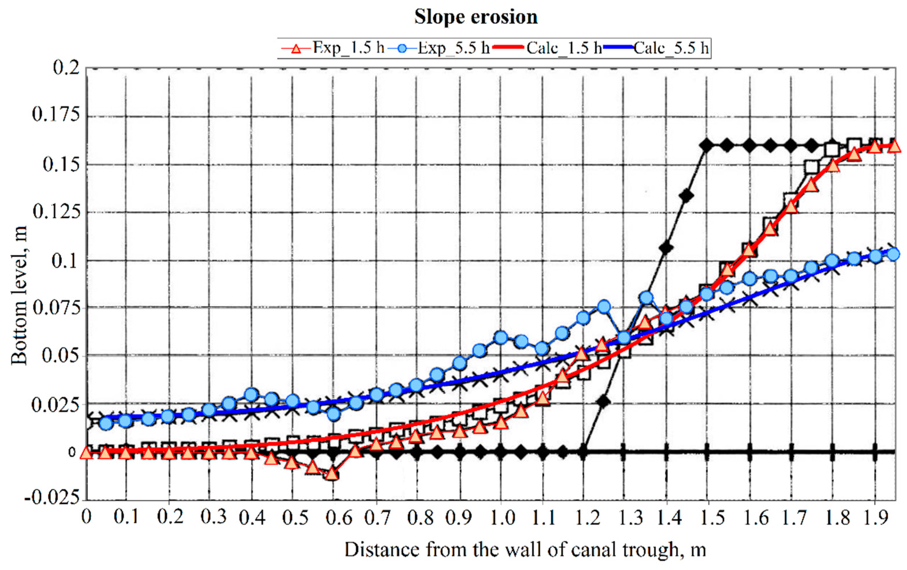
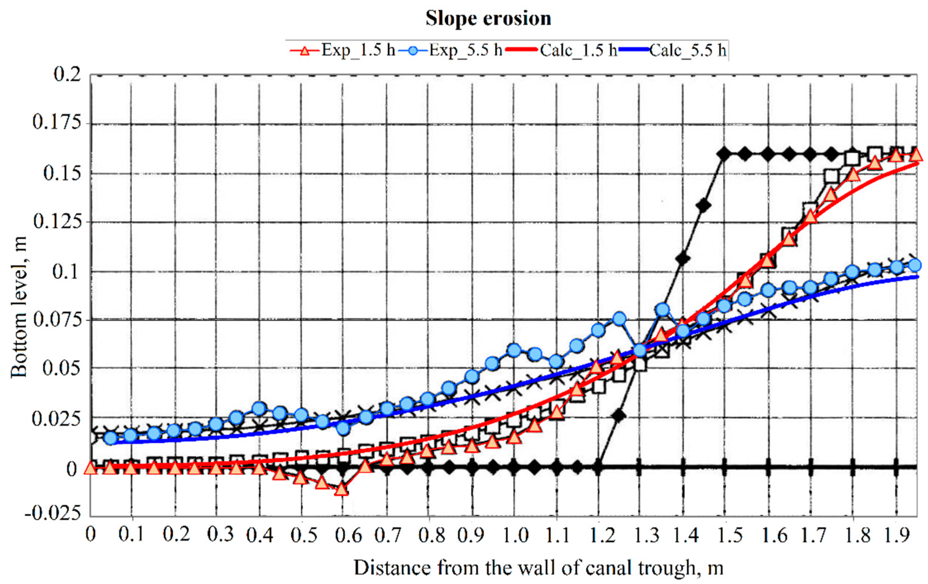
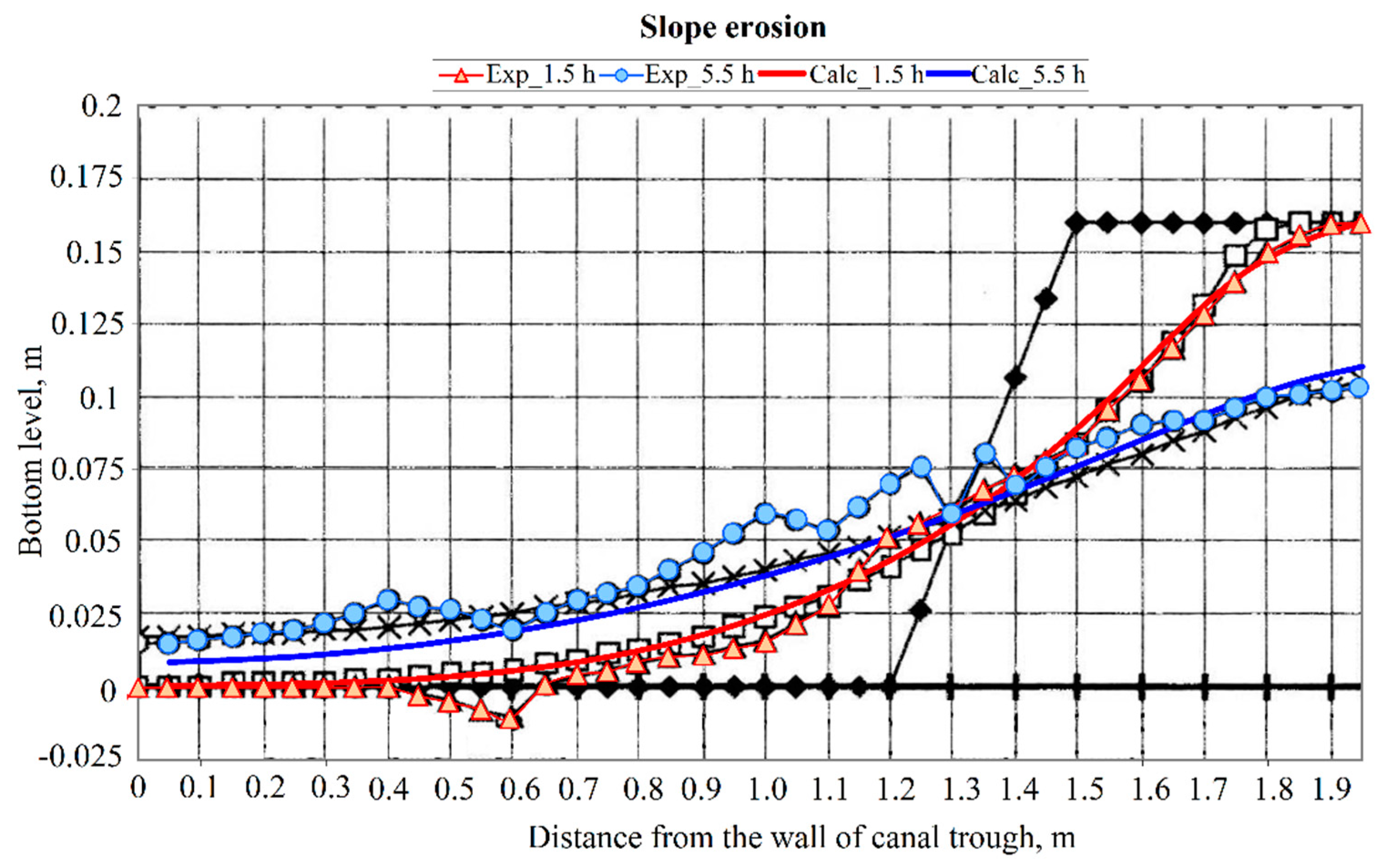
• Numerical studies were conducted to investigate the channel deformation, providing insights into the nature and intensity of these deformations. A comparison with the experimental data demonstrated a good agreement with the experimental results. However, it is worth noting that the optimal values of the empirical coefficients varied between the different experiments, highlighting the need for further work to establish more universal closing relations for the model.
• Verifying the model using field data is crucial for enhancing its applicability and reliability. Additionally, the extension of the model to account for hydraulically heterogeneous soils is a promising avenue because the concentration transfer equation (Equation 4) allows for independent calculations of different particle fractions, assuming that the total concentration of particles in the flow is not excessively high.

References

1. Belikov, V. V.; Zaitsev, A. A.; Militeev, A. N. Mathematical modeling of complex reaches of large river channels. Water Resources 2002, 29, 643–650. [Google Scholar] [CrossRef]
2. Ivanenko, S. A.; Koryavov, P. P.; Militeev, A. N. Modern computational technologies for calculating open flow dynamics. Water Resources 2002, 29, 518–530. [Google Scholar] [CrossRef]
3. Strelkoff, T. Numerical solution of Saint-Venant equations. Journal of the Hydraulics Division 1970, 96, 223–252. [Google Scholar] [CrossRef]
4. Cooley, R. L.; Moin, S. A. Finite element solution of Saint-Venant equations. Journal of the Hydraulics Division 1976, 102, 759–775. [Google Scholar] [CrossRef]
5. Bastin, G.; Coron, J. M.; d'Andréa-Novel, B. On Lyapunov stability of linearized Saint-Venant equations for a sloping channel. Networks and Heterogeneous Media 2009, 4, 177–187. [Google Scholar] [CrossRef]
6. Ying, X.; Khan, A. A.; Wang, S. S. Upwind conservative scheme for the Saint-Venant equations. Journal of Hydraulic Engineering 2004, 130, 977–987. [Google Scholar] [CrossRef]
7. Liu, H.; Wang, H.; Liu, S.; Hu, C.; Ding, Y.; Zhang, J. Lattice Boltzmann method for the Saint–Venant equations. Journal of Hydrology 2015, 524, 411–416. [Google Scholar] [CrossRef]
8. Litrico, X.; Fromion, V.; Baume, J. P.; Arranja, C.; Rijo, M. Experimental validation of a methodology to control irrigation canals based on Saint-Venant equations. Control Engineering Practice 2005, 13, 1425–1437. [Google Scholar] [CrossRef]
9. Belikov, V. V.; Zaitsev, A. A.; Militeev, A. N. Numerical modeling of flow kinematics in a segment of inerodable channel. Water Resources 2001, 28, 640–648. [Google Scholar] [CrossRef]
10. Saleh, F.; Ducharne, A.; Flipo, N.; Oudin, L.; Ledoux, E. Impact of river bed morphology on discharge and water levels simulated by a 1D Saint–Venant hydraulic model at regional scale. Journal of Hydrology 2013, 476, 169–177. [Google Scholar] [CrossRef]
11. Brisset, P.; Monnier, J.; Garambois, P. A.; Roux, H. On the assimilation of altimetric data in 1D Saint–Venant river flow models. Advances in Water Resources 2018, 119, 41–59. [Google Scholar] [CrossRef]
12. Kader, M. Y. A.; Badé, R.; Saley, B. Study of the 1D Saint-Venant equations and application to the simulation of a flood problem. Journal of Applied Mathematics and Physics 2020, 8, 1193. [Google Scholar]
13. Vila, J. P.; Chazel, F.; Noble, P. 2D versus 1D models for shallow water equations. Procedia IUTAM 2017, 20, 167–174. [Google Scholar] [CrossRef]
14. Fernandez-Nieto, E. D.; Marin, J.; Monnier, J. Coupling superposed 1D and 2D shallow-water models: Source terms in finite volume schemes. Computers & Fluids 2010, 39, 1070–1082. [Google Scholar]
15. Chen, Y.; Wang, Z.; Liu, Z.; Zhu, D. 1D–2D coupled numerical model for shallow-water flows. Journal of Hydraulic Engineering 2012, 138, 122–132. [Google Scholar] [CrossRef]
16. Morales-Hernández, M.; García-Navarro, P.; Burguete, J.; Brufau, P. A conservative strategy to couple 1D and 2D models for shallow water flow simulation. Computers & Fluids 2013, 81, 26–44. [Google Scholar]
17. Ongdas, N.; Akiyanova, F.; Karakulov, Y.; Muratbayeva, A.; Zinabdin, N. Application of HEC-RAS (2D) for flood hazard maps generation for Yesil (Ishim) River in Kazakhstan. Water 2020, 12, 2672. [Google Scholar] [CrossRef]
18. Mihu-Pintilie, A.; Cîmpianu, C. I.; Stoleriu, C. C.; Pérez, M. N.; Paveluc, L. E. Using high-density LiDAR data and 2D streamflow hydraulic modeling to improve urban flood hazard maps: A HEC-RAS multi-scenario approach. Water 2019, 11, 1832. [Google Scholar] [CrossRef]
19. Shustikova, I.; Domeneghetti, A.; Neal, J. C.; Bates, P.; Castellarin, A. Comparing 2D capabilities of HEC-RAS and LISFLOOD-FP on complex topography. Hydrological Sciences Journal 2019, 64, 1769–1782. [Google Scholar] [CrossRef]
20. Thalakkottukara, N. T.; Thomas, J.; Watkins, M. K.; Holland, B. C.; Oommen, T.; Grover, H. Suitability of the height above nearest drainage (HAND) model for flood inundation mapping in data-scarce regions: A comparative analysis with hydrodynamic models. Earth Science Informatics 2024, 1–15. [Google Scholar] [CrossRef]
21. Vazquez-Cendon, M. E.; Cea, L.; Puertas, J. The shallow water model: The relevance of geometry and turbulence. Monografias de la Real Academia de Ciencias de Zaragoza 2009, 31, 217–236. [Google Scholar]
22. Nadaoka, K.; Yagi, H. Shallow-water turbulence modeling and horizontal large-eddy computation of river flow. Journal of Hydraulic Engineering 1998, 124, 493–500. [Google Scholar] [CrossRef]
23. Pu, J. H. Turbulence modelling of shallow water flows using Kolmogorov approach. Computers & Fluids 2015, 115, 66–74. [Google Scholar]
24. Camporeale, C.; Canuto, C.; Ridolfi, L. A spectral approach for the stability analysis of turbulent open-channel flows over granular beds. Theoretical and Computational Fluid Dynamics 2012, 26, 51–80. [Google Scholar] [CrossRef]
25. Becchi, I. Considerations on the limits of integration field of de Saint Venant's equation for free surface flows. Meccanica 1972, 7, 147–150. [Google Scholar] [CrossRef]
26. Militeev, A. N.; Bazarov, D. R. A two-dimensional mathematical model of the horizontal deformations of river channels. Water Resources 1999, 26, 17–21. [Google Scholar]
27. Bazarov, D.; Markova, I.; Raimova, I.; Sultanov, S. Water flow motion in the vehicle of main channels. IOP Conference Series: Materials Science and Engineering 2020, 883, 012001. [Google Scholar] [CrossRef]
28. Lyatkher, V. M.; Militeev, A. N.; Togunova, N. P. Investigation of the distribution of currents in the lower pools of hydraulic structures by numerical methods. Hydrotechnical Construction 1978, 12, 585–593. [Google Scholar] [CrossRef]
29. Bazarov, D.; Vatin, N.; Norkulov, B.; Vokhidov, O.; Raimova, I. Mathematical model of deformation of the river channel in the area of the damless water intake. In Springer International Publishing 2022, pp. 1–15.
30. Duc, B. M.; Wenka, T.; Rodi, W. Numerical modeling of bed deformation in laboratory channels. Journal of Hydraulic Engineering 2004, 130, 894–904. [Google Scholar] [CrossRef]
31. Duan, J. G.; Julien, P. Y. Numerical simulation of meandering evolution. Journal of Hydrology 2010, 391, 34–46. [Google Scholar] [CrossRef]
32. Darby, S. E.; Alabyan, A. M.; Van de Wiel, M. J. Numerical simulation of bank erosion and channel migration in meandering rivers. Water Resources Research 2002, 38. [Google Scholar] [CrossRef]
33. Wang, B.; Xu, Y. J.; Xu, W.; Cheng, H.; Chen, Z.; Zhang, W. Riverbed changes of the uppermost Atchafalaya River, U.S.A.—A case study of channel dynamics in large man-controlled alluvial river confluences. Water 2020, 12, 2139. [Google Scholar] [CrossRef]
34. Kaveh, K.; Reisenbüchler, M.; Lamichhane, S.; Liepert, T.; Nguyen, N. D.; Bui, M. D.; Rutschmann, P. A comparative study of comprehensive modeling systems for sediment transport in a curved open channel. Water 2019, 11, 1779. [Google Scholar] [CrossRef]
35. Kim, Y.; Choi, G.; Park, H.; Byeon, S. Hydraulic jump and energy dissipation with sluice gate. Water 2015, 7, 5115–5133. [Google Scholar] [CrossRef]
36. Gladkov, G.; Habel, M.; Babiński, Z.; Belyakov, P. Sediment transport and water flow resistance in alluvial river channels: Modified model of transport of non-uniform grain-size sediments. Water 2021, 13, 2038. [Google Scholar] [CrossRef]
37. Wang, S.; Yang, B.; Chen, H.; Fang, W.; Yu, T. LSTM-based deformation prediction model of the embankment dam of the Danjiangkou Hydropower Station. Water 2022, 14, 2464. [Google Scholar] [CrossRef]
38. Qi, H.; Yuan, T.; Zhao, F.; Chen, G.; Tian, W.; Li, J. Local scour reduction around cylindrical piers using permeable collars in clear water. Water 2023, 15, 897. [Google Scholar] [CrossRef]
39. Jiang, H.; Zhao, B.; Dapeng, Z.; Zhu, K. Numerical simulation of two-dimensional dam failure and free-side deformation flow studies. Water 2023, 15, 1515. [Google Scholar] [CrossRef]
40. Bai, Y.; Xu, H. A study on the stability of laminar open-channel flow over a sandy rippled bed. Science China Series E-Technological Sciences 2005, 48, 83–103. [Google Scholar] [CrossRef]
41. Dalla Barba, F.; Picano, F. Direct numerical simulation of the scouring of a brittle streambed in a turbulent channel flow. Acta Mechanica 2021, 232, 4705–4728. [Google Scholar] [CrossRef]
42. Camporeale, C.; Canuto, C.; Ridolfi, L. A spectral approach for the stability analysis of turbulent open-channel flows over granular beds. Theoretical and Computational Fluid Dynamics 2012, 26, 51–80. [Google Scholar] [CrossRef]
43. Becchi, I. Considerations on the limits of integration field of de Saint Venant's equation for free surface flows. Meccanica 1972, 7, 147–150. [Google Scholar] [CrossRef]
Figure 1. The washed-out model, (a) the working part view, (b) the 3-dimensional overall model, (c) the principal scheme of the working part.
Preprints 144555 g001
Figure 2. Bottom marks and rectangular grid for a numerical model of an eroded slope.
Preprints 144555 g002
Figure 3. Flattening the slope when calculating the diffusion coefficient (6) from the bottom concentration (12) and non-shear velocity according to formula (9): β =40, α 1 = 0.25 .
Preprints 144555 g003
Figure 4. Slope flattening when calculating the diffusion coefficient based on bottom concentration (12) and non-shear velocity using formula (10): β=15, α 1 = 0.25 .
Preprints 144555 g004
Figure 5. Slope leveling when calculating the diffusion coefficient based on bottom concentration (12) and non-shear velocity using formula (10): β = 30 , α 1 = 0.25 .
Preprints 144555 g005