1. Introduction
The world is undergoing a significant transition away from fossil fuels, embracing modern renewable energy technologies to meet its escalating energy needs and demands. Bioenergy, derived from sources such as woody biomass, agricultural residues, and organic materials and waste, is pivotal in this paradigm shift, constituting the largest share (two−thirds) of global renewable energy utilization [
1]. It is anticipated that bioenergy continues to have a decisive share in future net zero emission scenarios and that its contribution to energy supply will further increase. This transition underscores the growing significance of biomass energy within the global energy landscape. However, it is worth noting that billions of people still rely on the inefficient use of traditional biomass for cooking and heating [
1]. The combustion of biomass produces air pollutants similar to those emitted by fossil fuels, with the exception of sulfur oxides [
2]. Furthermore, research has shown that the health impacts attributed to emissions from biomass and wood combustion can be more harmful than those from fossil fuels [
3]. These emissions primarily result from incomplete biomass combustion and the release of solid particulate matter.
The adoption of woody biomass and non-wood biomass such as agricultural residues, coupled with efficient combustion energy technologies, holds the potential to substantially reduce harmful emissions into the atmosphere while increasing its contribution to energy supply, making it a viable alternative to fossil fuels. Due to efficiency increase as compared to traditional biomass use, it is an important cornerstone of future scenarios. Despite significant investments in the research and development of biomass energy technologies, a knowledge gap persists, particularly concerning efficient, low cost determination of biomass properties, including its elemental compositions (carbon (C), hydrogen (H), nitrogen (N), oxygen (O), sulfur (S) and others). During inefficient and incomplete combustion, harmful pollutants such as carbon monoxide, sulfur oxides (SOx), nitrogen oxides (NOx), along with particulate matter (PM
2.5 and PM
10) are continuously released into the environment as smoke, posing significant health risks through indoor and outdoor exposure, with women and children being the most vulnerable [
4,
5,
6].
The elemental composition of biomass has a profound impact on combustion efficiency and the emission levels released into the environment. These emissions, in turn, carry significant consequences for both the energy industry and the natural surroundings. Energy release during biomass combustion correlates positively with carbon and hydrogen contents, as they are the primary contributors to its energy value [
7]. High carbon content is desirable for energy production [
8], and hydrogen's high energy content makes it valuable [
9]. During combustion, oxygen reacts with carbon and hydrogen, reducing the available energy in biomass. Elevated oxygen and nitrogen contents decrease the calorific value, thereby reducing energy potential [
10]. Nitrogen and sulfur are undesirable elements in biomass due to their contribution to the formation of harmful NOx and sulfur dioxide [
11,
12]. To minimize environmental impact and ensure sustainable operation and maintenance of combustion systems, low sulfur content in biomass is preferred [
12]. Hence, it is crucial to rapidly, accurately, and non-invasively assess the elemental composition of biomass, including C, N, O, H, and S. This assessment is essential for understanding biomass elemental composition and the potential emissions risks during energy production.
In our
previous research [
13], an investigation was conducted into the application of NIR spectroscopy (NIRS) for the comprehensive analysis of the ultimate analysis parameters of ground biomass intended for energy utilization. The study concludes that NIRS offers a reliable and non-destructive alternative method for rapidly assessing the elemental composition of ground biomass for energy−related purposes. Despite the valuable findings from previous research, these finding primarily served academic and research institutions. However, biomass normally is made into pellet form for export and to increase energy density where the grinding is necessary before making pellets Woodchips are especially useful, as they are easy to use and some time, ground wood is not suitable in power operations due to the high cost and length of time necessary for sample preparation, therefore, it is a popular source of energy for power plants because of low preparation costs [
14]. Meanwhile, woodchip quality could be more effectively examined to achieve higher levels of plant efficiency [
14]. Hence, this study aims at improving the applicability of NIR spectroscopy to assess the ultimate analysis parameters of chipped biomass, i.e. biomass with particle sizes commonly found in industrial applications. In consequence, this research outcome may directly benefit traders and energy companies, facilitating the utilization of research outcomes without the need for extensive biomass preparation such as grinding.
The data structure of samples used for model development in this present work were in two forms i.e. non-wood and wood samples. As reported, the non-wood and wood species were different in their lignocellulosic constituents. Non−wood material of agricultural waste compost of lignin, holocellulose, α−cellulose, pentosan and ash [
15]. For example, agricultural residues, such as hemp and sugarcane bagasse, contained higher concentrations of cellulose and lower levels of recalcitrant lignin when compared to the average woody biomass [
16,
17]. However, Hawanis et. al [
18] reported the non-wood contained lower cellulose and lignin while wood contained higher [
19,
20]. Therefore, the wider range of energy parameters such as heating value and definitely the ultimate analysis parameters, C, H, N, O and S. This may make the model more robust. Though, the effect of combined non-wood and wood spectra of biomass chips on rapid prediction of ultimate analysis parameters using NIR spectroscopy was investigated in this study.
Literatures which were explored in the Google Scholar data up to end 2023 base showed a few research has combined the non−wood such as agricultural residue and agricultural industrial residue and forest residue e.g., leaves, barks and so on and wood such as fast-growing tree and wood from forest. Generally, only one specific species of biomass was used for prediction modeling and the determination of ultimate analysis constituents by NIR spectroscopy was rarely reported. Only two reports were found including Posom and Sirisomboon [
22], who optimized the PLS models using NIR spectra of 80 bamboo chip samples for evaluation of C, H, N, S and O content. The models showed the coefficient of determination of prediction set (R
2P) and ratio of prediction to deviation (RPD) of 0.803 and 2.31 for C; 0.856 and 2.65 for H; 0.973 and 6.6 for N; 0.785 and 2.19 for S and 0.522 and 1.46 for O, respectively. Similarly, the models developed by Zhang et al. (2017) [
23] using 100 accessions of sorghum biomass with R
2P of 0.96 for wt.% of C, 0.87 for wt.% of H, 0.86 for wt.% of N, and 0.83 for wt.% of O.
There were two reports found in the available data base that developed a model for two similar species to evaluate ultimate analysis parameters, C, H, N, O and S. A total of 222 rice straw and wheat straw, collected from 24 provinces of China, were used for NIRS calibration and validation in this study where R
2P and standard error of predictions (SEP) of independent validation were, respectively, 0.97 and 0.37% for C, 0.77 and 0.17% for H, 0.87 and 0.10% for N [
24]. Saha et al [
25] developed models by using 276 wood chip ground samples of pine tree of two species (Loblolly (
Pinus taeda) and slash (
Pinus elliottii)) where the biomass spectra (400 to 2498 nm at 2−nm intervals). The samples were a mix of bark, branch, needle, wood or whole tree biomass. The prediction results show for C (sample number (n) = 43; coefficient of R
2P = 0.90; RPD = 3.14; ratio of prediction to interquartile (RPIQ) = 3.23); for N (n = 44; R
2P = 0.95; RPD = 4.33; RPIQ = 5.96); and for S (n = 42; R
2P = 0.93; RPD = 3.67; RPIQ = 3.24).
There were two reports of our group contributed the research results of NIR prediction models for ultimate analysis parameters of the non-wood and wood samples including Pitak et al [
26] who developed the PLS regression using the spectra obtained by line-scan NIR hyperspectral imager in which the most effective model for the prediction of C, H and N content of 160 non−wood and wood biomass pellets including filter cake (15 pellets),
Leucaena leucocepphala (10 pellets), bamboo (15 pellets), cassava rhizome (15 pellets), bagasse (15 pellets), sugarcane leaves (15 pellets), straw (15 pellets), rice husk (15 pellets), eucalyptus bark (15 pellets), napier grass (15 pellets) and corn cob (15 pellets) developed using iGA wavelength selection and standard normal variate (SNV) spectral pretreatment and provided the highest accuracy with R
2Pp and SEP of 0.83 and 1.33% for C; 0.84 and 0.17% for H and 0.90 and 0.098% for N; respectively. The second report was contributed by Shrestha et al [
13] where the ground non-wood and wood samples spectra which were 110 samples of agricultural residues and 90 samples of fast−growing trees were used to develop the PLSR models combined with multi-preprocessing methods for ultimate analysis showed R
2P and RPD for C of 0.7217 and 1.9, for N of 0.8410 and 2.7, for H of 0.7678 and 2.1 and for O of 0.6289 and 1.7, respectively.
The main objectives of this research include:
- (1)
develop PLSR models using NIR raw spectra, traditional preprocessing, MP 5−range, MP 3−range, GA, and SPA for assessing chip biomass properties for energy usage by employing NIRS while the spectra of the biomass were from non−wood (agricultural residue and bamboo) and wood (fast growing trees) samples.
- (2)
compare the performance of the PLSR models based on R2C, RMSEP, R2P, RMSEP, RPD, and bias.
- (3)
study the effect of combined non-wood and wood species in model development on model performance by scatter plot analysis.
- (4)
select the better performing PLSR−based model for each ultimate analysis parameter, compared with the performance of the ground biomass for rapidly assessing biomass properties for energy usage.
- (5)
determine the limit of quantification (LOQ) value of the proposed model calibration set for each ultimate analysis parameter in chip biomass.
3. Results and Discussion
Table 1 shows the number of non-wood samples and wood samples in calibration set and validation set. The wood sample number is about 33-35% of total sample number, hence, non-wood samples number is 65-67%. Out of 120 samples, the number of outlier samples can be evaluated by the data in
Table 1.
Table 2 presents statistical data for the ultimate analysis parameters of chip biomass obtained using CHNS/O elemental analyzer (Thermo ScientificTM FLASH 2000). This data was used in both the calibration and prediction sets
for model development. S content in the chip biomass was not detected, possibly due to its very low content falling below the detection threshold. Therefore, a PLSR−based model for S content in the chip biomass was not developed in this study. The wt.% of O is calculated using equation (1).
Table 3 shows results of the PLSR-based model for ultimate analysis (wt.%) of chip biomass, where bolded model showing the best performance. However, it is essential to consider the recommendation provided by Williams et al. [
34], where with an R
2P value between 0.66-0.81, the model can be used for rough screening and other suitable calibration purposes. Therefore, C, O and N model were. For H model, by Williams et al. guideline [
34], a model with a R
2P value between 0.50−0.64 is only suitable for very rough screening. Likewise, every model of biomass chips for ultimate analysis parameters was in alignment with the recommendation from Zornoza et al. [
35], which any model with an RPD value below 2 was deemed insufficient for any application.
3.1. wt.% of C
Table 3 presents the results of the PLSR−based model within the full wavenumber range of 3594.87–12,489.48 cm
−1 for the wt.% C of chip biomass, with the best−performing model highlighted in bold.
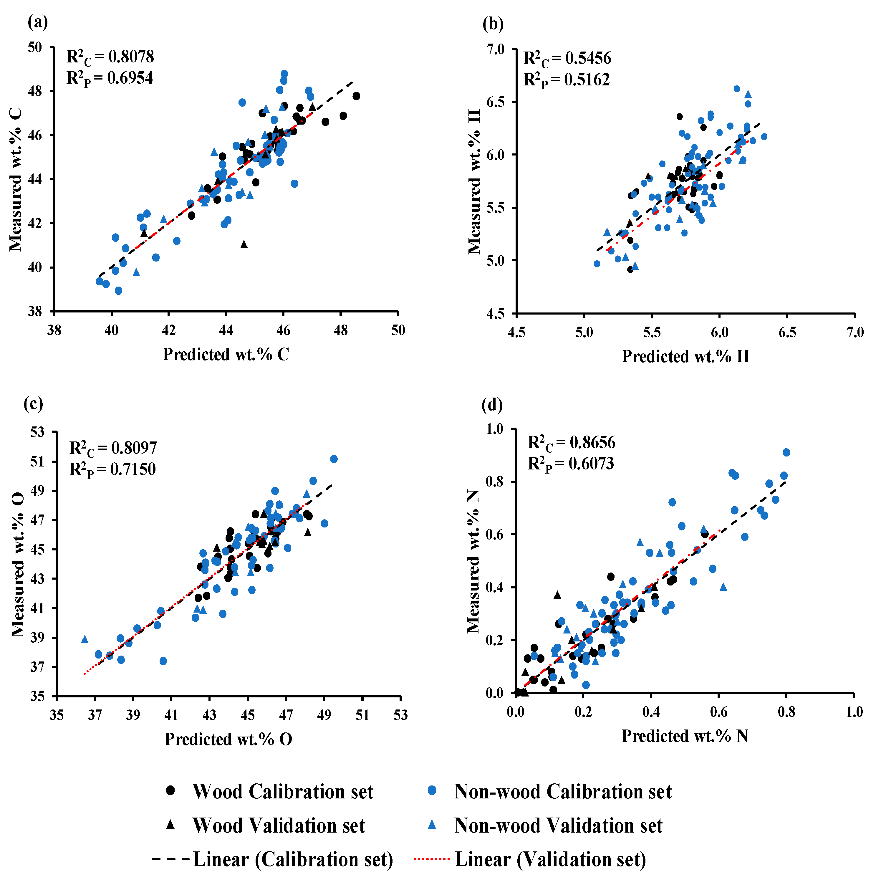
The model, developed using GA−PLSR with spectrum preprocessing involving the sd2, a gap, and segments of five each, along with nine LVs, provided better results. It achieved R2C, RMSEC, R2P, RMSEP, RPD, and bias values of 0.8078, 0.9320 wt.%, 0.6954, 1.1252 wt.%, 1.8, and 0.0053 wt.%, respectively. By determining RMSEP, these results represent a 6.8566 % improvement in the model performance compared to Full−PLSR. Utilizing equation (3), the LOQ value was calculated as 9.3724 wt.% for C. Notably, the LOQ value is lower than the minimum wt.% C value used during model development, indicating that the model exhibits high sensitivity and can reliably detect and quantify wt.% C starting from 9.3724 wt.%.
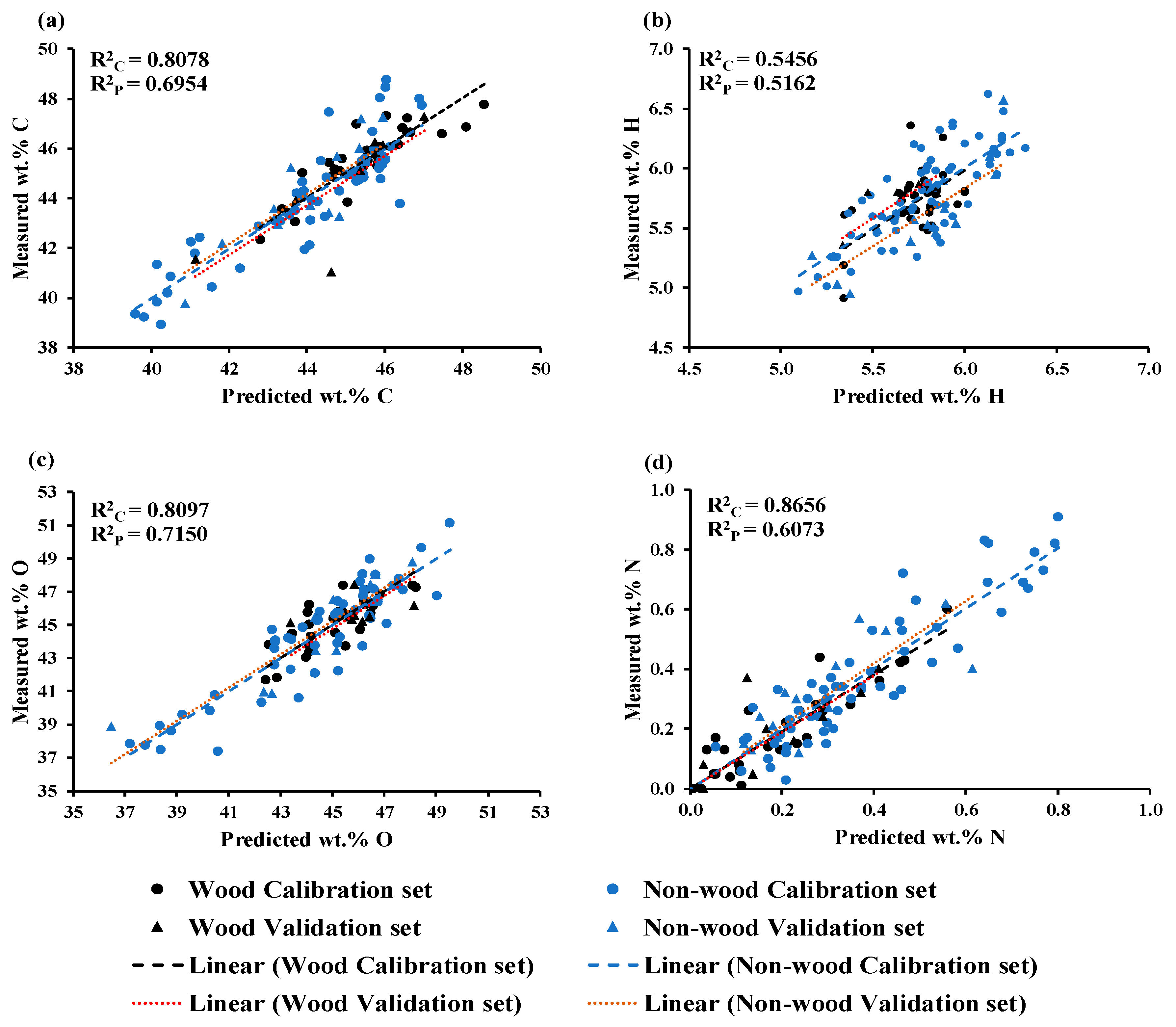
Figure 2a shows a scatter plot comparing the predicted and measured wt.% of C, which was obtained using GA−PLSR. The trend line for the prediction set and calibration set is overlap indicating same slope. The slope shows the rate of change of Y (measured value) as a function of the rate of change of X (predicted values) [
34] or vice versa, hence, indicating predicted values of both sets of data have changed with the same rate and this characteristic is same for the models for O and N shown in
Figure 2c,d.
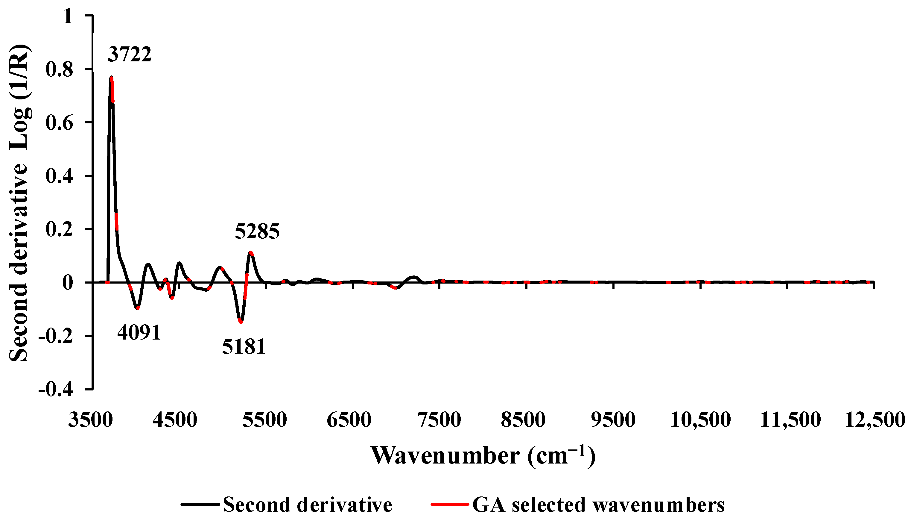
Figure 3 displays the average sd2 absorbance values obtained after preprocessing, highlighting 306 selected wavenumbers (marked in red) identified through GA. These wavenumbers fall within the full spectral range of 3594.87–12,489.48 cm
−1. Peaks were observed at 3722, 4091, 5181, and 5285 cm
−1, all of which might have the potential to enhance the model's performance. The wavenumbers 3722 cm
−1 and 4091 cm
−1 are associated with the C−H aromatic functional group, specifically C−H aryl material type. The peak at 5181 cm
−1 corresponds to a combination of O−H stretching and HOH bending, indicative of polysaccharides. Similarly, the peak at 5285 cm
−1 is associated with the functional group of O−H hydrogen bonding between water and exposed polyvinyl alcohol OH groups [
36].
Previous studies by Zhang et al. [
37] and Posom and Sirisomboon [
38] have demonstrated that vibrational bands related to C−H aromatic, C−H stretching, N−H stretching, N−H deformation, O−H stretching, HOH bending, O−H hydrogen bonding, and similar factors play a crucial role in predicting the wt.% of C in various biomass varieties. These findings align with the vibration bands observed in our study, providing support for our results and suggesting that these selected peaks likely have a significant influence on the model performance.
3.2. wt.% of H
The model developed using GA−PLSR with vector normalization as preprocessing showed the best performance with 11 LVs (
Table 3). It selected 67 important wavenumbers using GA. The model's performance, in terms of R
2C, RMSEC, R
2P, RMSEP, RPD, and bias values, was 0.5456, 0.02336 wt.%, 0.5162, 0.2322 wt.%, 1.5, and −0.0781 wt.%, respectively. Compared with Full−PLSR, the GA improved the PLSR model accuracy by 1.6743 %.
The LOQ value was calculated as 2.3484 wt.%, which is lower than the minimum reference value used for the model development. This suggests that the selected model is sensitive and can sensitively quantify H from 2.3484 wt.%.
Figure 2b displays a scatter plot comparing the predicted and measured wt.% of H, which was obtained using GA−PLSR. It is clear that the trend line for the prediction set exhibits an offset in relation to the trend line of the calibration set and the 45−degree line. This offset raises concerns about the model constant bias along the range of the data indicating the over−estimating model.
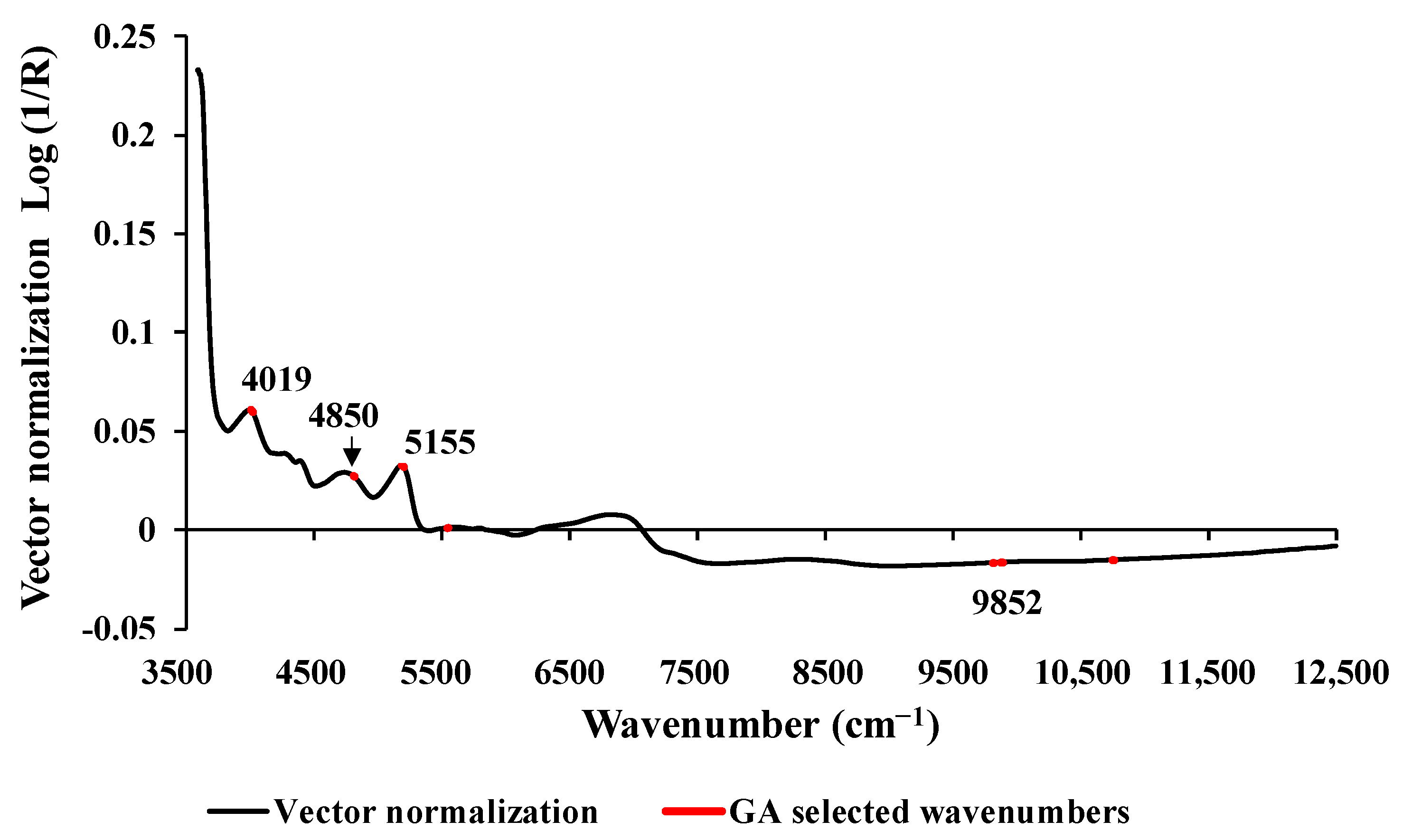
Figure 4 displays the average absorbance values within the range of 3594.87–12,489.48 cm
−1. These values were obtained after preprocessing using vector normalization and highlight 67 selected wavenumbers, marked in red, which were identified using GA. Significant peaks were observed at the wavenumbers 4019, 4850, 5155, and 9852 cm
−1, respectively, and these may have an influence on the model performance. The peak at 4019 cm
−1 is associated with the spectra−structure combination of C–H stretching and C–C stretching, with the material type being cellulose. The peak at 4850 cm
−1 corresponds to the functional group of N–H combination bands found in secondary amides within proteins. The peak at 5155 cm
−1 is related to the combination of O–H stretching and HOH bending, with the material type being water. Finally, the peak at 9852 cm
−1 is associated with the second overtone of the fundamental stretching band of N–H asymmetric stretching, and the material type is aromatic amine [
36].
In comparison to previous studies conducted by Shrestha et al. [
13], Zhang et al. [
37], and Posom and Sirisomboon [
38] that focused on measuring the wt.% of H in biomass using NIRS, our study discovered similar peaks within the range of 4000−9900 cm
−1 and vibration bands such as O–H stretching, HOH bending, C–H stretching, and C–C stretching. Therefore, our study findings align with these earlier studies on this specific aspect.
However, when evaluating the overall performance of various PLSR−based models, this study suggests that the wt.% of H was not sufficiently explained by the vibration of those mentioned bonds.
3.3. wt.% of O
Assuming that the S content in chip biomass is negligible, as its wt.% is too low to be detected by the instrument, we calculated the wt.% of O in the chip biomass for 120 samples using equation (1). The wt.% of ash content for each biomass was determined using a TGA.
Table 3 presents the optimal results from five different types of PLSR−based models. The most effective model was developed using the MP PLSR 5−range method, incorporating a spectral preprocessing combination set of 2, 5, 2, 1, and 5, which corresponded to the following ranges: 3625.72–5392.30 cm
−1 with SNV, 5400.02–7166.59 cm
−1 with the sd2, 7174.31–8940.89 cm
−1 with SNV, 8948.60–10,715 cm
−1 with raw spectra, and 10,722.9–12,489.48 cm
−1 with the sd2. This model employed 15 LVs.
Figure 2c illustrates the scatter plot comparing measured versus predicted wt.% of O obtained from the MP PLSR 5−range method. This method yielded R
2C of 0.8097, RMSEC of 1.2366 wt.%, R
2P of 0.7150, RMSEP of 1.3088 wt.%, RPD of 1.9, and a bias of 0.0733 wt.%. Compared with Full−PLSR method performance, the MP PLSR 5−range method significantly improved the model accuracy by 11.4913 %. The LOQ value for wt.% of O was calculated as 12.4424 wt.%, which is lower than the minimum wt.% of O used during model development. This indicates that the model is highly sensitive and can accurately quantify O content in chip biomass from 12.4424 wt.%.
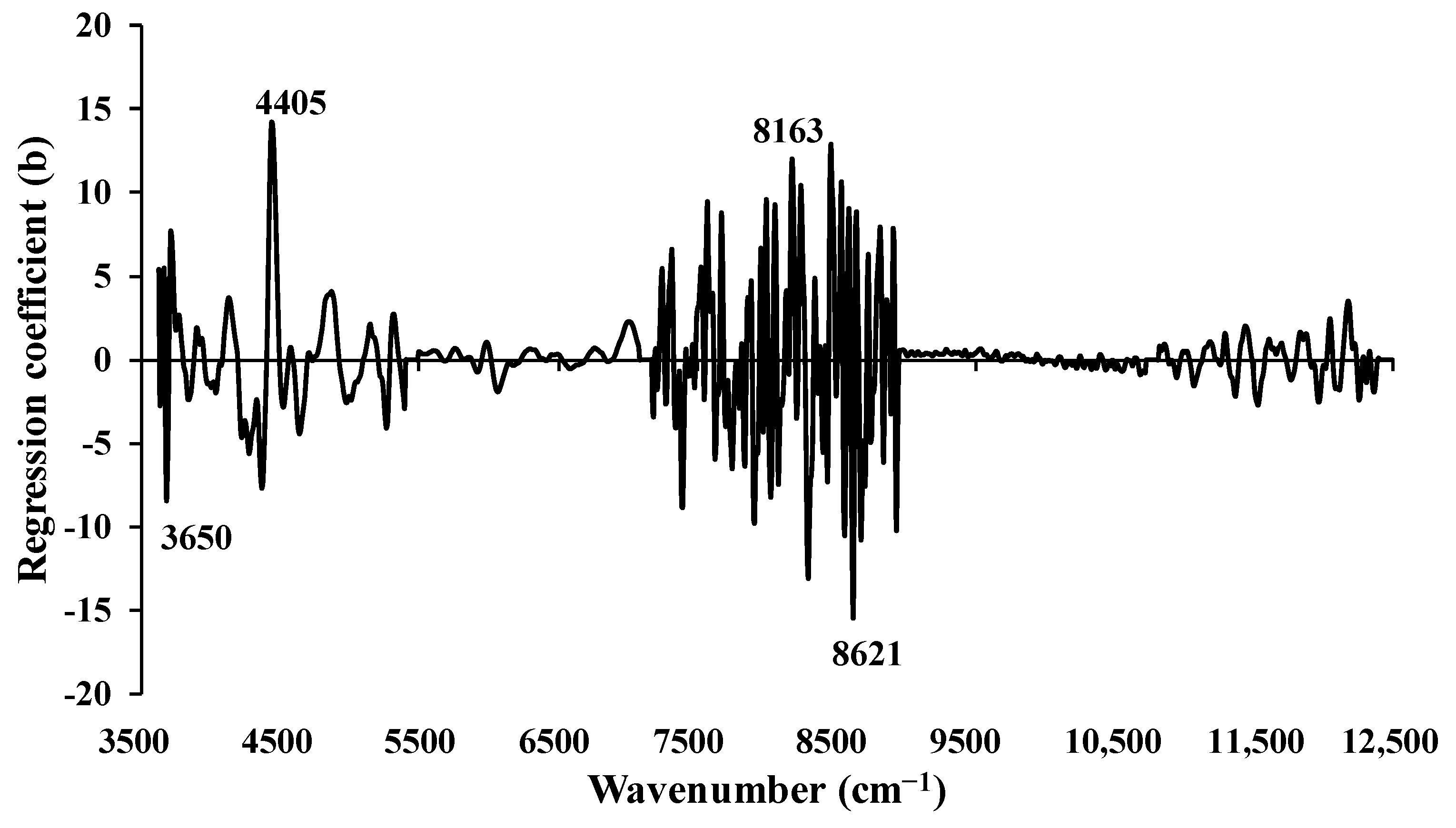
Figure 5 displays the regression coefficient plot for wt.% of O content in chip biomass, obtained from the MP PLSR 5−range method. Several notable peaks were observed at 3650, 4405, 8163, and 8621 cm
−1, each potentially exert a significant influence on the model’s performance. Specifically, the peak at 3650 cm
−1 corresponds to the O–H functional group found in the primary alcohols, characterized by the fundamental stretching vibrational absorption band of O–H. The peak at 4405 cm
−1 represent the combination of O–H stretching and C–O stretching, with cellulose as the material type. The peaks at 8163 cm
−1 and 8621 cm
−1 are associated with the second overtone of the fundamental stretching band of C–H and the fourth overtone of the fundamental stretching band of C=O, respectively, which are typically found in hydrocarbons and aliphatic compounds [
36].
When compared with previous studies on wt.% of O in biomass, such as those by Shrestha et al. [
13], Zhang et al. [
37], and Posom and Sirisomboon [
38], this study reveals some contradictory peaks. However, the vibrational bands, such as O−H from primary alcohol, C=O stretching, and C−H stretching, among others, were similar. These finding supports the research result of this study, suggesting that the significant peaks observed in this study have an impact on the development of the model for assessing wt.% of O in chip biomass.
3.4. wt.% of N
The best model for rapid prediction of wt.% of N was obtained using the MP PLSR 3−range method with a spectral preprocessing combination set of 4, 0, and 0 (
Table 3). This set corresponds to the sd1 from 3594.87 to 5492.59 cm
−1, and zero absorbance from 7498.314 to 12,489.48 cm
−1.
Figure 2d illustrates the scatter plot of measured versus predicted wt.% of N content in the chip biomass, obtained from the MP PLSR 3−range method with 15 LVs, the best−performing model achieved an R
2C of 0.8656, RMSEC of 0.0820 wt.%, R
2P of 0.6073, RMSEP of 0.1008 wt.%, RPD of 1.6, and a bias of 0.0191 wt.%. These results indicate that within the range 3594.87-5492.59 cm
−1 (refer
Figure 6), by effectively correcting baseline shifts, and assigning zero absorbance value within the remaining wavenumber range, the model performance is enhanced. Compared with full−PLSR
using RMSEP value, the MP PLSR 3−range method improved the model performance by 2.5473%. However, based on R2C and R2P values, the selected model indicates overfitting. This suggests that out model fits the training data too closely, capturing noise and irrelevant patterns that do not hold true in the other dataset. Therefore, we highly recommend research for the error occurred during scanning and reference measurement.
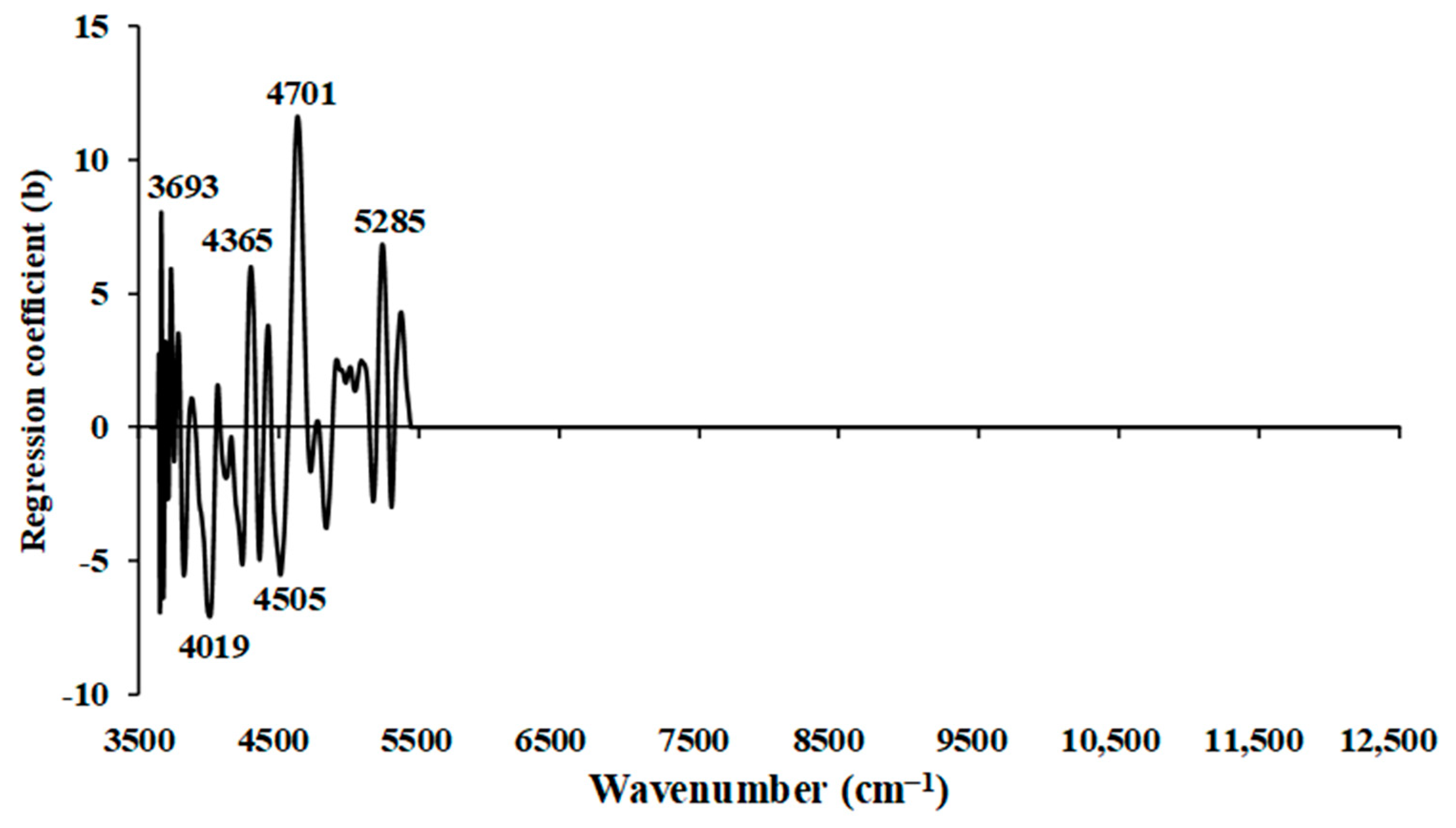
Figure 6 illustrates the regression coefficient plot for the wt.% of N in chip biomass, obtained using the multi−preprocessing PLSR 3−range method. Significant peaks that could potentially influence the model performance were observed within the wavenumber range of 3594.87–5492.59 cm
−1 only. These significant peaks were noticed at wavenumbers 3693, 4019, 4365, 4505, 4701, and 5285 cm
−1. Specifically, the peak at 3693 cm
−1 is associated with function group of C–H aromatic C–H bands, characterized by the material type C–H aryl. At 4019 cm
−1, the peak represents functional groups with a combination of C–H stretching and C–C stretching from cellulose as the material type.
The peak at 4365 cm−1 corresponds to CONH2, specifically due to C=O bonded to the N–H of the peptide link termed the α−helix structure. The peak at 4505 cm−1 is associated with the N–H combination band. Similarly, the peak at 4701 cm−1 corresponds to the function group of N–H/C=O combination from polyamide II. Lastly, the peaks at 5285 cm−1 are associated with O–H hydrogen bonding between water and exposed polyvinyl alcohol OH. These peaks are crucial in understanding the composition of the chip biomass and are important for model development and analysis. Furthermore, in the range of 7498.314–12,489.48 cm−1, the regression coefficient value equals zero. This indicates an insufficient linear relationship between the dependent (spectral information) and independent (reference value) variables in this range, and it does not significantly contribute to the predictive model for prediction of wt.% of N.
The previous study conducted by Posom and Sirisomboon [
38], which aimed to evaluate the wt.% of N in bamboo, also revealed significant peaks within the range of 4424 to 6920 cm
−1. Similarly, Shrestha et al. [
13] conducted a study on wt.% of N in ground biomass from the same source and exhibited important peaks within a similar range, specifically within 4019 to 6711 cm
−1. This finding aligns with the results of our study, providing additional support for our research. It is noteworthy that in both studies, common vibrational bands, such as N–H stretching, C=O stretching, C–H stretching, C–C stretching, aromatic C–H, and O–H bonds between water and alcohol, among others, were identified. This consistency in vibration bonds reinforces our study findings and suggests that these specific peaks likely play a crucial role in influencing the model performance.
4. Effect of non-wood and wood samples on model performance
Table 4 shows the reference values of wt.% of C, H, N and O of non-wood and wood samples in calibration and validation sets. From
Figure 2 and
Table 4, it is obvious that the range of every element content is wider after the two sets were combined for modeling. Therefore, the models can now be regarded as robust models. From
Figure 2a,c the range of wt.% of C and O of wood samples was narrower than those of the non-wood samples which were extended more to the lower wt%.
Figure 2d illustrates in the opposite way where the value range of N of wood samples was lower and narrower than those of the non-wood samples. Therefore, models for wt% of C, O and N were better performance than that of H model. The wood sample reference values of H were group together and more or less had the same range to the range of non-wood samples. (
Figure 2b).
Literatures show that the one specie model of non-wood which were bamboo wood chips [
22] and sorghum [
23] for evaluation of ultimate analysis parameters, C, H, N, O and S had better performance than our combined non-wood and wood model as the results described in Introduction of this manuscript. Similarly, the two similar species of rice straw and wheat straw model [
24] and pine tree of two species (Loblolly (
Pinus taeda) and slash (
Pinus elliottii)) model [
25] indicated the better prediction performance, though they were homogeneous ground samples which might make their model performance better than the chip ones due to less scattering problem. Shrestha et al [
13] worked with ground samples of the same batch of non-wood and wood samples. Spectra from this experiment showed better R
2P and RPD for C, N, H and O which is clamied to be due to the same merit of homogeneous samples.
Using larger biomass particles sizes, Pitak et al [
26] combined the non−wood and wood biomass pellet NIR spectra obtained by averaging every pixel spectrum of the pellets from hyperspectral image (HSI). This approach provided better performance in predicting elements from the ultimate analysis than our model, i.e. in detail data collection by the HSI leads to significant improvements.
Figure 7 shows the scatter plots of the highest performance models in this study in predicting the C, H, O and N content of the wood and non-wood samples which is same as
Figure 2 but the different is
Figure 7 shows the simple regression lines of each group of non-wood and wood samples both for calibration set and prediction set. For better vision,
Table 5 shows the numeric data of R
2, slope, intercept calculated from the scatter plots of wood and non-wood calibration and prediction sets. Williams et al explained that the slope of the trend line plotted between Y (measured value) and X (NIR predicted value) indicated the rate of change of Y as a function of the rate of change of X [
34]. The intercept of different species illustrated the same trend as slope interpretation especially when the slope is more than 1 the intercept was with minus sign and if less than 1 the intercept was with plus sign. While the slope was 1 the intercept was low closed to zero and when the slope was more or less than 1 the intercept was high far from zero.
The perfect relationship of the reference values and the predicted values is when the correlation coefficient (R) and slope equal to 1 and the intercept equal to zero [
34].
From
Table 5, for C model, the non-wood samples contributed slightly more merit on calibration model performance than wood samples for more R and slope was more closed to 1 and intercept was more closed to zero. But the prediction set of non-wood provided steeper slope and intercept far more from zero.
By the same way of interpretation, the model for H got more merit from non-wood samples, while the wood samples, the R of the trend line was very low and the slope was far from 1 and the intercept was slightly far from zero. The incongruous of the trend lines of both sets make overall performance of the model worst as shown in
Table 3.
For N model, the wood and non-wood calibration set samples more or less had the same trend line characteristics which supplement the good calibration model performance, though the prediction sample set of both biomass species trend line characteristics shows less R and slope far from 1 led to overfit calibration models of both biomass groups (
Table 5).
For O model, the non-wood group had better trend line characteristics contributed good merit to model while the poorer trend line characteristics of the wood group made the overall model inferior but by small portion due to the number of samples in non-wood group was much more (
Table 5). By the strong merit of non-wood group the overall model performance for O prediction was fairly acceptable (
Table 3).
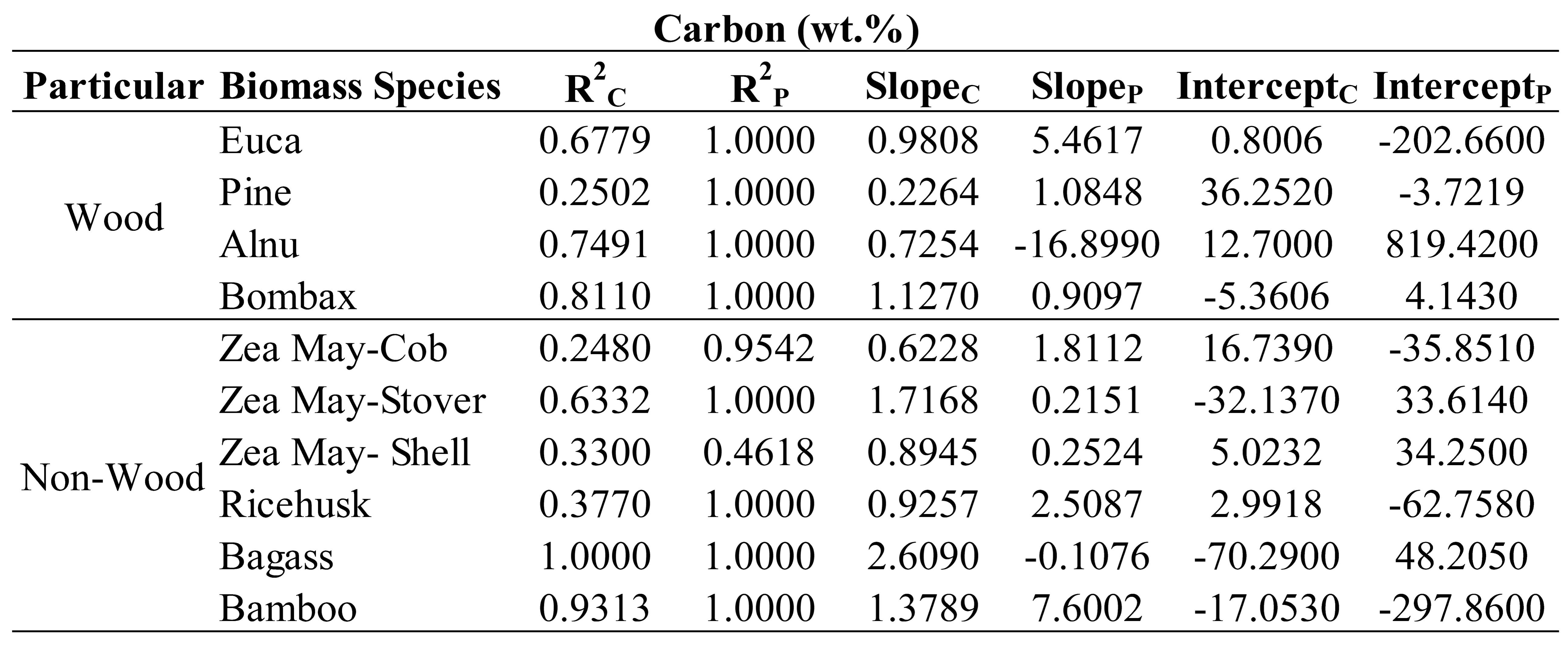
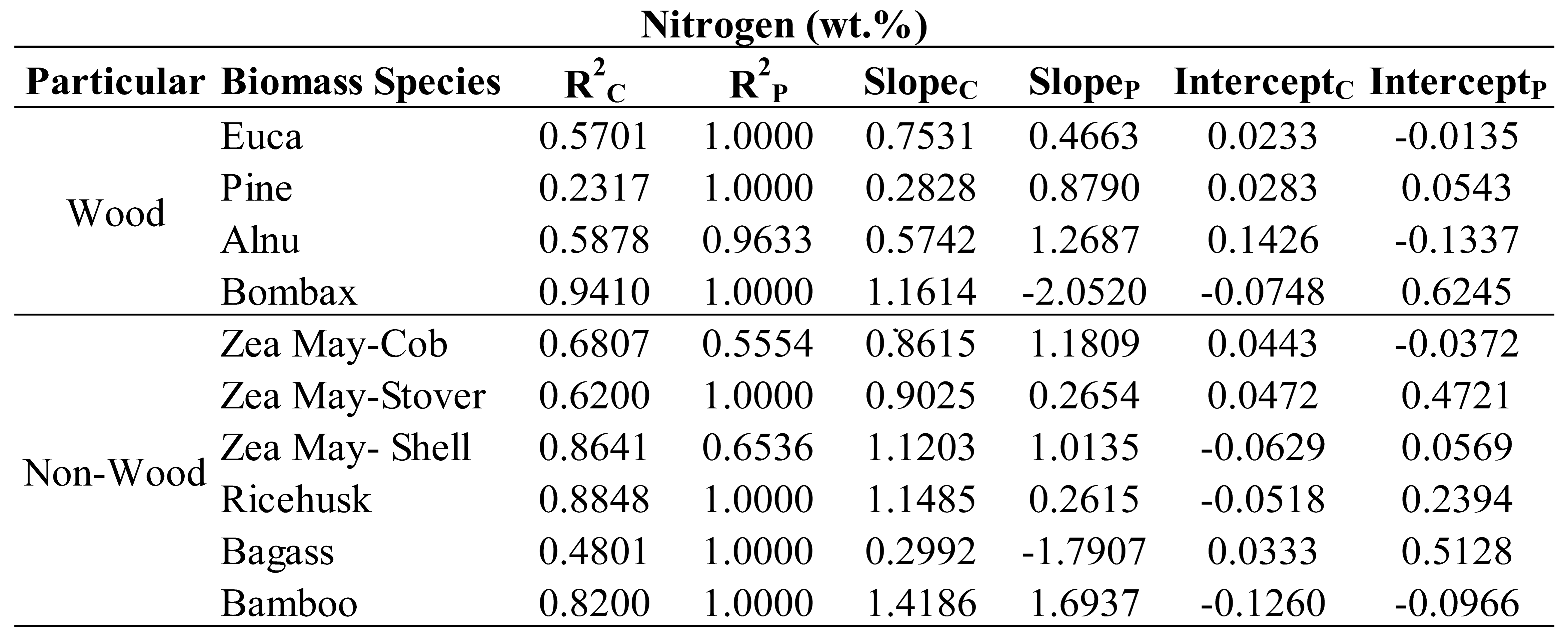
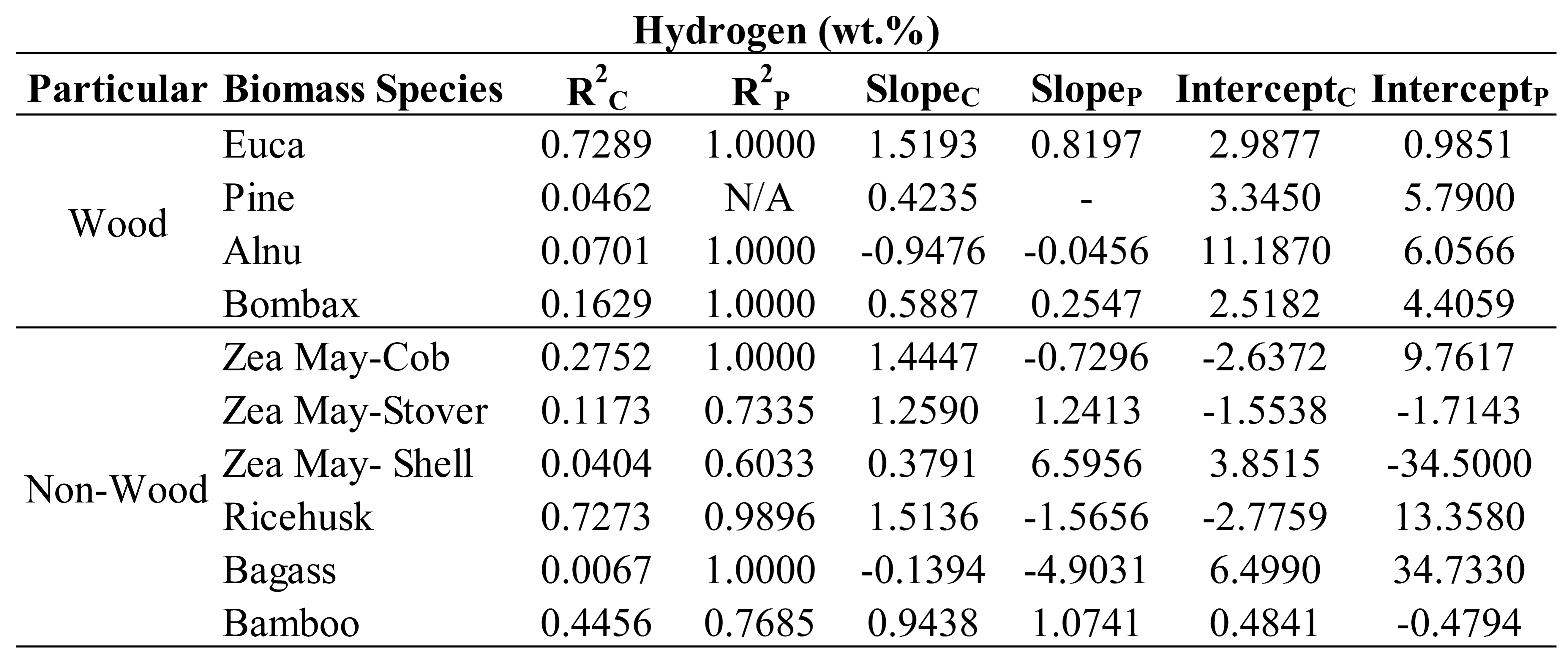
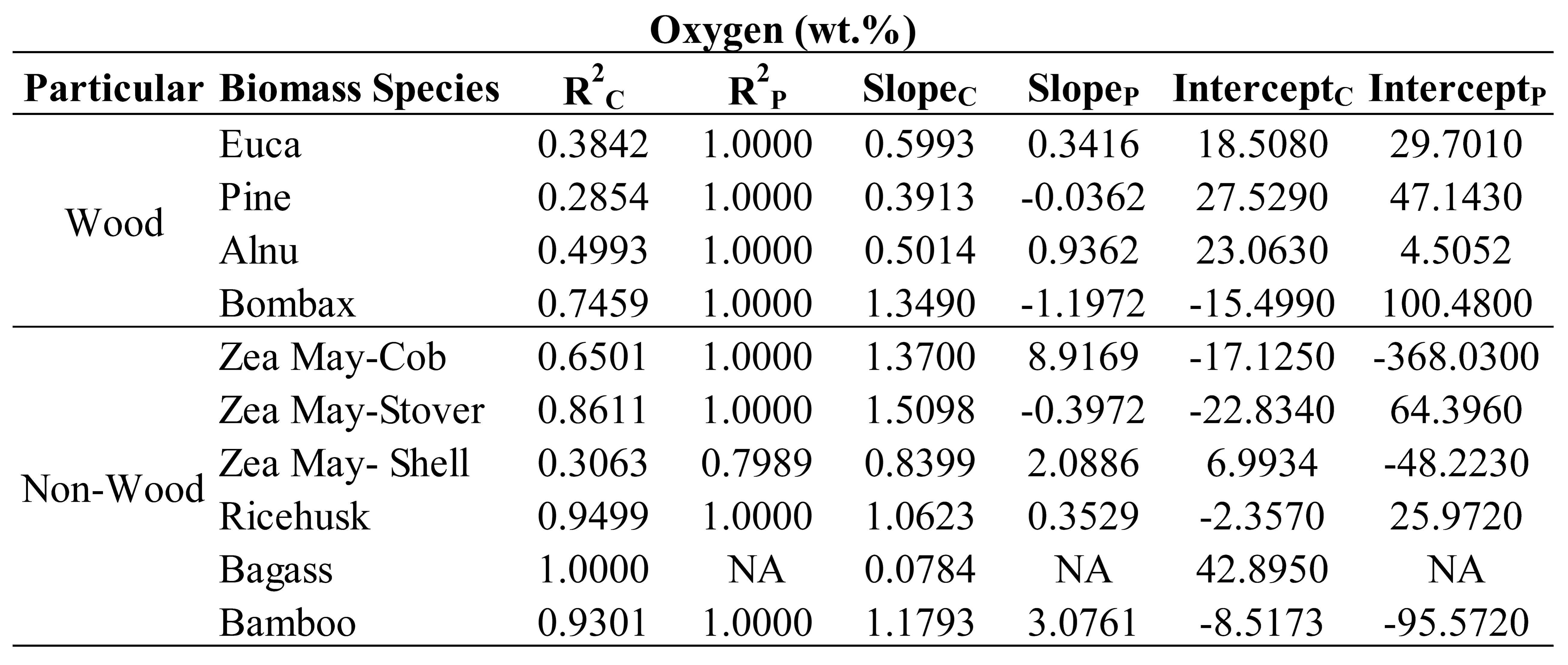
Table 6,
Table 7,
Table 8 and
Table 9 show the trend line characteristics including R
2, slope and intercept of each specific plant of wood and non-wood samples used in the optimized models for evaluation of C, N, H and O, respectively. It was observed that most of the R
2P of every plant was equaled to 1 for the samples of those plants in the optimized model was only 2 samples connected to straight line. Therefore, we ignored to interpret the trend line characteristics of prediction set and only R
2C , slope and intercept of calibration set will be interpreted. As indicating by Williams et al [
34] when the R approached to 1 and slope approached to 1 and intercept approached to zero, the model was approached excellent. Therefore, to include different species in a model the species have to be not only in the different values of the constituents to make a wider range for robust model but also they must provide the characteristic of the same rate of change of NIR predicted values with the measured values (same slope and slope should approached to 1 and intercept is same (no gap) and approached zero). As expected, the trend of R
2, of slope and of intercept of different species were not the same for their different characteristics. However, some species which their characteristics were similar, the trends were in common but depend on the element the model was used for prediction.
From
Table 6,
Table 7,
Table 8 and
Table 9, as expected the intercept of different species illustrated the same trend as slope interpretation especially when by the fact, the slope is more than 1 the intercept was with minus sign and if less than 1 the intercept was with plus sign. While the slope was 1 the intercept was low closed to zero and when the slope was more or less than 1 the intercept was high far from zero.
Therefore, the following were the effects of specific species on performance of the optimized models interpreted by scatter plot analysis using the R2 and slope of the trend line of the specific plant in the model developed.
For C (
Table 6), by R
2C interpretation, most of non-wood species (agricultural waste) except bagasse and bamboo show un-acceptable trend lines compared to wood species samples except pines. Therefore, to include the mentioned non-wood species caused the poor effect on C model. By interpretation of slope, there were 3 groups of slope (by value round up) i.e. 1 including Eucalyptus, Alnus and Bombax in wood species and corn cob, corn shell, rice husk and bamboo in non-wood species, less than 1 including pine in wood specie and more than 1 including corn stover and bagasse indicating unequal slope different species in the same optimized model show the effect of specific species on model performance. These can be summarized that for model to be better, pine and corn stover should not be included in modeling for C prediction.
By the same way of interpretation, from
Table 7, the optimized model for N, pine and bagasse should be not included, from
Table 8, for H, pine, Alnus, corn shell and bagasse should not be included and from
Table 9, for O, pine should not be included for better performance of the models. These were due to the poor both R and slope of the eliminated species which were not in accordance with the other species.
These results show that the different species affected the model performance of each parameter prediction in a different manner and by scatter plot analysis which of these species were affecting the model negatively and how to improve the model performance were indicated.
5. Comparison of model performance between using chipped and ground biomass spectra
In this section, the model performance of chipped biomass for ultimate analysis parameters to the model of ground biomass [
13] derived from the same sample varieties is compared. The comparison is based on the metrics R
2C, RMSEC, R
2P, RMSEP, and RPD. The results demonstrate that chipped biomass generally performs less effectively in these models compared to ground biomass, except for wt.% of O.
For wt.% of C and wt.% of H, both chipped and ground biomass models demonstrated better performance when employing the GA−PLSR model. This outcome aligns with expectations, as GA optimizes feature selection to maximize fitness, while PLSR maximizes covariance between absorbance values and areas of interest [
39].
For wt.% of C, the GA−PLSR model applied to ground biomass yield an R
2C of 0.7851, RMSEC of 0.9753 wt.%, R
2P of 0.7217, RMSEP of 0.9740 wt.%, and RPD of 1.93 [
13]. In contrast, the model applied to chipped biomass performed less effectively (refer
Table 2). Therefore, it is recommended to adopt the GA−PLSR model with sd2 preprocessing on ground biomass when evaluating wt.% of C.
Similarly, the GA−PLSR model applied to ground biomass outperforms that of chipped biomass for wt.% of H. Ground biomass yielded an R
2C of 0.8814, RMSEC of 0.1041 wt.%, R
2P of 0.7678, RMSEP of 0.1434 wt.%, and RPD of 2.14 [
13], whereas chipped biomass lagged behind (refer
Table 2). Hence, for wt.% of H, the GA−PLSR model with spectral preprocessing from SNV on ground biomass is recommended.
Regarding wt.% of N, the MP PLSR 5−range method exhibited superior model performance on ground biomass, as evidenced by R
2C, RMSEC, R
2P, RMSEP, and RPD values of 0.8682, 0.0675 wt.%, 0.8410, 0.0973 wt.%, and 2.65, respectively [
13], when compared to chipped biomass performance obtained from the MP PLSR 3−range method (refer
Table 2). This underscores the suitability of ground biomass for evaluating wt.% of N.
Surpricingly, in contrast, for wt.% of O, the model derived from chipped biomass excelled, despite both models utilizing the MP PLSR 5−range method. In ground biomass, R
2C, RMSEC, R
2P, RMSEP, and RPD values were 0.6674, 1.4461wt.%, 0.6289, 1.5275 wt.%, and 1.71 respectively [
13], which fell short of chipped biomass results. Hence, it is recommended to adopt the MP PLSR−5 range method with the preprocessing combination set of 2, 5, 2, 1, and 5 for assessing wt.% of O in chipped biomass. This could be due to ash determination where ash directly influences %O determination based on Eq 1. Also, ash is typically accumulating in small particles, i.e. time of grinding in conjunction with subsampling can have an influence on ash determination.
All the above comparison and findings underscore the importance of selecting the appropriate PLSR−based model for precise analysis of ultimate analysis parameters, depending on the specific parameter of interest. There could be several factors that contribute to the lower performance of the chipped biomass model, which can be addressed to improve the model performance. The key contributing factor to this performance difference is obviously the particle size of the biomass samples. Chipped biomass typically consists of larger and different sizes of particles, leading to increased scattering of NIR light during sample scanning [
40]. Consequently, the spectra generated from chipped biomass can be of lower quality, resulting in weaker correlations between spectral data and reference data [
41]. Additionally, ground biomass exhibits a more compact and uniform sample structure, reducing the likelihood of NIR light leakage during scanning. Another significant factor affecting the lower model performance is the moisture content in biomass samples. Chipped biomass often contains higher moisture levels, and water has the property of absorbing NIR light in the near−infrared region [
42]. This NIR absorption interferes with the measurements and can introduce inaccuracies, particularly for elements like C, H, O and N.
In the chipped biomass models, it is evident that the performance of the prediction set consistently lags behind that of the calibration set. This suggests that the model closely overfits the calibration data, capturing both valuable information and noise or random variations [
43]. In the machine learning context, Cawley and Talbot [
44] emphasized that overfitting in model selection is likely to be most severe when the sample size is small and the number of hyperparameters to be tuned is relatively large [
45]. Like in our case, the number of latent variables of the best models were high.
Consequently, when new samples are introduced into the prediction set, the model may struggle to generalize and provide accurate predictions. Furthermore, the presence of outliers in the prediction set, which were not accounted for in the calibration set, can further negatively impact the model performance [
46].
The performance of ground biomass is better compared to chipped biomass due to several factors. Ground biomass allows for better sample homogenization, ensuring uniformity and consistent composition. Additionally, it offers more control over sample thickness, as chips may vary in thickness, affecting accuracy. Moreover, ground samples reduce light scattering effects and enables improved penetration of the NIRS signal, allowing for precise and accurate logging of spectral information.
6. Conclusion
In this study, PLSR−based models were developed and compared using FT−NIRS to analyze the ultimate analysis parameters of combined non-wood and wood chip biomass, specifically focusing on wt.% of C, H, O, and N content. All chipped biomass samples were scanned within 3594.87−12,489.48 cm−1 on the diffuse reflectance with sphere macro sample rotating mode, with a particular emphasis on their suitability for energy application. The model with the optimum performance was selected based on trade off parameters of R2C, RMSEC, R2P, RMSEP, RPD and bias.
The optimum model performance analysis reveals that the model selected for predicting the wt.% of C, H, N, and O in chipped biomass are suitable primarily for initial rough screening. It is recommended to adopt the multi−preprocessing PLSR 5−range method chipped biomass model for wt.% of O content analysis as an alternative method for rapid assessment. However, for evaluation of wt.% of C, H, and N content, the chipped biomass model performance falls short of the model developed for ground biomass by Shrestha et al. [
13]. Thus, it is advisable to use the chipped biomass model solely for initial screening before biomass trading. For a more comprehensive and accurate analysis, it is recommend grinding the chip biomass samples and employing the GA−PLSR model with sd1 for wt.% of C, GA−PLSR with SNV for wt.% of H and the multi-preprocessing PLSR 5−range method with combination set of 4, 4, 5, 3, and 4 for wt.% of N, as developed by Shrestha et al. [
13].
The LOQ values for C, H, and O were below the model minimum reference value, demonstrating high model sensitivity. However, the LOQ value for N exceeds the minimum reference value, indicating the model detection limit to the minimum value in the calibration sample set range.
By analysis of scatter plot of measured constituent and NIR predicted constituent, the effect of including different biomass species (non-wood and wood species) in the modeling samples was studied. It was concluded that to include different species in a model, the species had to be not only in the different values of the constituents to be predicted to make a wider range for robust model but also the different sample species must provide the same rate of change of NIR predicted values with the measured values in the scatter plot (same slope and slope approached to 1 and intercept is same (no gap) and approached zero) for the high performance model if R is approached to one. The results show that the different species affected on model performance of each parameter prediction in a different manner and by scatter plot analysis, which of the species affecting the model negatively were identified and dictated how to improve the model performance.
Author Contributions
B.S.; conceptualization, methodology, software, formal analysis, investigation, resources, data curation, writing the original draft, writing–review & editing. J.P.; conceptualization, software, formal analysis, data curation, writing–review & editing, supervision. P.S.; conceptualization, data curation, writing the original draft, writing–review & editing, validation, supervision, project administration, funding acquisition. B.P.S.; conceptualization, writing–review & editing, and supervision. A.F.; writing–review & editing, visualization, supervision. All authors have read and agreed to the published version of the manuscript.
Figure 1.
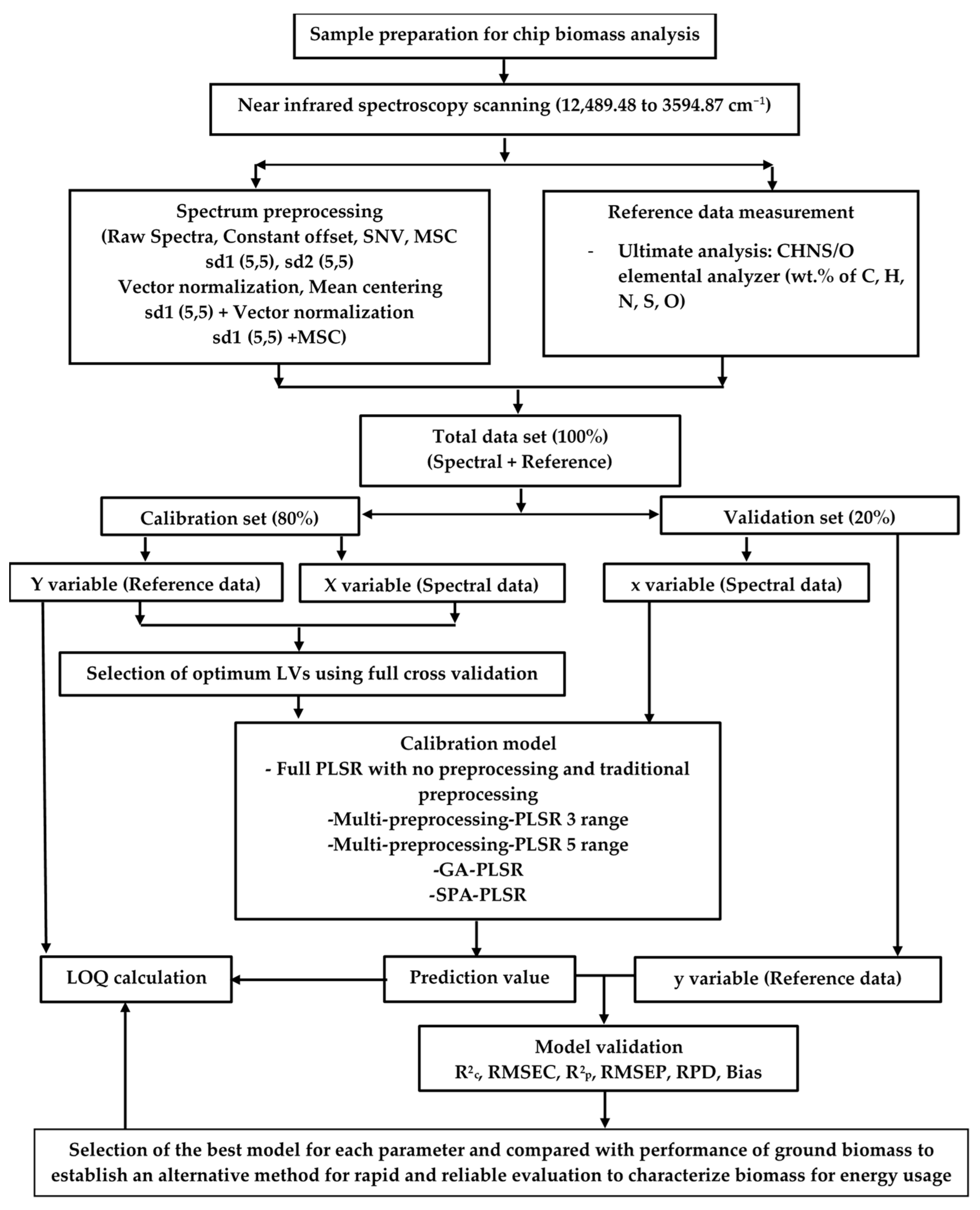
Flowchart of the overall research methodology for the rapid prediction of the ultimate analysis parameters of chip biomass for energy usage by NIRS using PLSR.
Figure 1.
Flowchart of the overall research methodology for the rapid prediction of the ultimate analysis parameters of chip biomass for energy usage by NIRS using PLSR.
Figure 2.
Measured versus predicted value in calibration and prediction sets for (a) wt.% of C, (b)wt.% of H, (c) wt.% of O, and (d) wt.% of N.
Figure 2.
Measured versus predicted value in calibration and prediction sets for (a) wt.% of C, (b)wt.% of H, (c) wt.% of O, and (d) wt.% of N.
Figure 3.
The second derivative absorbance value of studied biomass obtained using the sd2 preprocessing with a selection of important wavenumber obtained from GA for prediction of wt.% of C, within the full wavenumber range of 3594.87 −12,489.48 cm−1.
Figure 3.
The second derivative absorbance value of studied biomass obtained using the sd2 preprocessing with a selection of important wavenumber obtained from GA for prediction of wt.% of C, within the full wavenumber range of 3594.87 −12,489.48 cm−1.
Figure 4.
The vector normalization absorbance value of studied biomass obtained using the vector normalization preprocessing with a selection of important wavenumber obtained from GA for prediction of wt.% of H, within the full wavenumber range of 3594.87 −12,489.48 cm−1.
Figure 4.
The vector normalization absorbance value of studied biomass obtained using the vector normalization preprocessing with a selection of important wavenumber obtained from GA for prediction of wt.% of H, within the full wavenumber range of 3594.87 −12,489.48 cm−1.
Figure 5.
The regression coefficient for the wt.% O of chip biomass using the MP PLSR 5−range method.
Figure 5.
The regression coefficient for the wt.% O of chip biomass using the MP PLSR 5−range method.
Figure 6.
The regression coefficient for the wt.% N of chip biomass using the MP PLSR 3−range method.
Figure 6.
The regression coefficient for the wt.% N of chip biomass using the MP PLSR 3−range method.
Figure 7.
The scatter plots of optimized model for wt% of C, H, O and N where the simple regression lines of non-wood group and wood group illustrated both in calibration set and validation set.
Figure 7.
The scatter plots of optimized model for wt% of C, H, O and N where the simple regression lines of non-wood group and wood group illustrated both in calibration set and validation set.
Table 1.
The number of non-wood samples and wood samples in calibration set and validation set.
Table 1.
The number of non-wood samples and wood samples in calibration set and validation set.
| Parameter Total Sample |
Calibration set |
Validation set |
| Wood |
Non-Wood |
Total |
Wood |
Non-Wood |
Total |
| wt.% C |
111 |
31 |
58 |
89 |
8 |
14 |
22 |
| wt.% H |
119 |
32 |
63 |
95 |
8 |
16 |
24 |
| wt.% N |
116 |
31 |
62 |
93 |
9 |
14 |
23 |
| wt.% O |
102 |
28 |
54 |
82 |
8 |
12 |
20 |
Table 2.
The statistical data of the ultimate analysis parameters of the chip biomass obtained using CHNS/O elemental analyzer used in PLSR model development.
Table 2.
The statistical data of the ultimate analysis parameters of the chip biomass obtained using CHNS/O elemental analyzer used in PLSR model development.
| Parameter |
NT
|
Calibration set |
|
Validation set |
| NC
|
Max |
Min |
Mean |
SD |
|
NP
|
Max |
Min |
Mean |
SD |
| C (wt.%) |
111 |
89 |
48.7500 |
38.9300 |
44.6330 |
2.1380 |
|
22 |
47.2800 |
49.7550 |
44.4439 |
2.0878 |
| H (wt.%) |
119 |
95 |
6.6200 |
4.9100 |
5.7620 |
0.3485 |
|
24 |
6.5700 |
4.9500 |
5.6490 |
0.3411 |
| O (wt.%) |
102 |
82 |
51.1200 |
37.3600 |
44.6322 |
2.8521 |
|
20 |
48.8000 |
38.8500 |
45.1159 |
2.5149 |
| N (wt.%) |
116 |
93 |
0.9100 |
0.0000 |
0.2987 |
0.2250 |
|
23 |
0.6200 |
0.0000 |
0.2714 |
0.1645 |
Table 3.
Results of the PLSR-based model for ultimate analysis (wt.%) of chip biomass, bolded model showing the best performance.
Table 3.
Results of the PLSR-based model for ultimate analysis (wt.%) of chip biomass, bolded model showing the best performance.
| Parameter |
Algorithm |
Preprocessing |
LVs |
Calibration Set |
|
Prediction Set |
| R2C
|
RMSEC |
|
R2P
|
RMSEP |
RPD |
bias |
| wt.% C |
Full−PLSR |
Second derivative
(g = 5, s = 5) |
10 |
0.8215 |
0.8982 |
|
0.6489 |
1.2081 |
1.7 |
0.0854 |
| |
GA−PLSR |
Second derivative (SW:306) |
9 |
0.8078 |
0.9320 |
|
0.6954 |
1.1252 |
1.8 |
0.0053 |
| |
SPA−PLSR |
Second derivative (SW: 634) |
10 |
0.8030 |
0.9435 |
|
0.6520 |
1.2028 |
1.7 |
0.1036 |
| |
MP−PLSR: 3 range |
Combination set: 4,2,4 |
9 |
0.7132 |
1.1386 |
|
0.5514 |
1.3655 |
1.5 |
−0.1433 |
| |
MP−PLSR: 5 range |
Combination set: 4,1,4,3,1 |
13 |
0.8628 |
0.7875 |
|
0.5467 |
1.3727 |
1.5 |
−0.1226 |
| wt.% H |
Full−PLSR |
First derivative
(g = 5, s= 5) |
6 |
0.5086 |
0.2429 |
|
0.4996 |
0.2361 |
1.5 |
−0.0660 |
| |
GA−PLSR |
Vector normalization (SW: 67) |
11 |
0.5456 |
0.2336 |
|
0.5162 |
0.2322 |
1.5 |
−0.0781 |
| |
SPA−PLSR |
Second derivative (SW: 22) |
15 |
0.5172 |
0.2408 |
|
0.4478 |
0.2481 |
1.4 |
−0.0586 |
| |
MP−PLSR: 3 range |
Combination set: 5,5,0 |
7 |
0.5179 |
0.2406 |
|
0.4711 |
0.2428 |
1.4 |
−0.0644 |
| |
MP−PLSR: 5 range |
Combination set: 5,4,4,0,4 |
8 |
0.5964 |
0.2201 |
|
0.4877 |
0.2389 |
1.4 |
−0.0625 |
| wt.% O |
Full−PLSR |
Second derivative
(g = 5, s = 5) |
8 |
0.6243 |
1.7376 |
|
0.6362 |
1.4788 |
1.7 |
0.0814 |
| |
GA−PLSR |
Mean Centering (SW: 1025) |
11 |
0.6347 |
1.7134 |
|
0.6064 |
1.5381 |
1.6 |
0.2414 |
| |
SPA−PLSR |
Min−max normalization (SW:354) |
11 |
0.5800 |
1.8370 |
|
0.5815 |
1.5860 |
1.6 |
0.3466 |
| |
MP−PLSR: 3 range |
Combination set: 4,5,0 |
11 |
0.6572 |
1.6597 |
|
0.6153 |
1.5207 |
1.6 |
0.1064 |
| |
MP−PLSR: 5 range |
Combination set: 2,5,2,1,5 |
15 |
0.8097 |
1.2366 |
|
0.7150 |
1.3088 |
1.9 |
0.0733 |
| wt.% N |
Full−PLSR |
MSC |
10 |
0.7232 |
0.1177 |
|
0.5865 |
0.1035 |
1.6 |
−0.0065 |
| |
GA−PLSR |
SNV (SW: 39) |
10 |
0.5916 |
0.1429 |
|
0.5625 |
0.1064 |
1.5 |
−0.0132 |
| |
SPA−PLSR |
Min−max normalization (SW:413) |
7 |
0.6396 |
0.1343 |
|
0.5869 |
0.1034 |
1.6 |
−0.0190 |
| |
MP−PLSR: 3 range |
Combination set: 4,0,0 |
15 |
0.8656 |
0.0820 |
|
0.6073 |
0.1008 |
1.6 |
0.0191 |
| |
MP−PLSR: 5 range |
Combination set:1,4,4,1,0 |
7 |
0.6436 |
0.1335 |
|
0.5700 |
0.1055 |
1.5 |
0.0143 |
Table 4.
The range of wt.% of C, H, N and O of non-wood and wood samples in calibration and validation sets.
Table 4.
The range of wt.% of C, H, N and O of non-wood and wood samples in calibration and validation sets.
| Parameter |
Calibration set |
Validation set |
| Wood |
Non-Wood |
Wood |
Non-Wood |
| wt.% C |
47.77-42.33 |
48.75-39.93 |
47.28-41.02 |
47.24-39.76 |
| wt.% H |
6.36-4.91 |
6.62-4.97 |
6.57-4.95 |
5.87-5.36 |
| wt.% N |
0.60-0.00 |
0.91-0.00 |
0.40-0.00 |
0.62-0.12 |
| wt.% O |
47.40-41.68 |
51.12-37.36 |
47.43-45.14 |
48.80-38.85 |
Table 5.
The trend line characteristics of the wood and non-wood species in scatter plots of the best models for C, H, N, and O.
Table 5.
The trend line characteristics of the wood and non-wood species in scatter plots of the best models for C, H, N, and O.
| Element |
Wood |
|
Non-wood |
| R2C |
R2P |
SlopeC |
SlopeP |
InterceptC |
InterceptP |
|
R2C |
R2P |
SlopeC |
SlopeP |
InterceptC |
InterceptP |
| C |
0.7243 |
0.6456 |
0.8353 |
1.0139 |
7.5532 |
-0.8994 |
|
0.7962 |
0.7681 |
1.0243 |
1.2109 |
-1.0960 |
-9.1465 |
| H |
0.2683 |
0.5028 |
0.7876 |
0.7066 |
1.2085 |
1.7444 |
|
0.6111 |
0.7185 |
1.0342 |
1.1318 |
-0.1925 |
-0.9224 |
| N |
0.8335 |
0.5486 |
0.8915 |
0.7670 |
0.0197 |
0.0502 |
|
0.8454 |
0.6289 |
1.0368 |
0.8541 |
-0.0139 |
0.0708 |
| O |
0.6187 |
0.0992 |
0.8272 |
0.1840 |
7.8316 |
37.2740 |
|
0.8311 |
0.8063 |
1.0209 |
0.9519 |
-0.9462 |
2.3866 |
Table 6.
The trend line characteristics of specific biomass species for Carbon evaluation optimized model.
Table 6.
The trend line characteristics of specific biomass species for Carbon evaluation optimized model.
Table 7.
The trend line characteristics of specific biomass species for Nitrogen evaluation optimized model.
Table 7.
The trend line characteristics of specific biomass species for Nitrogen evaluation optimized model.
Table 8.
The trend line characteristics of specific biomass species for Hydrogen evaluation optimized model.
Table 8.
The trend line characteristics of specific biomass species for Hydrogen evaluation optimized model.
Table 9.
The trend line characteristics of specific biomass species for Oxygen evaluation optimized model.
Table 9.
The trend line characteristics of specific biomass species for Oxygen evaluation optimized model.
