
Submitted:
30 November 2023
Posted:
01 December 2023
You are already at the latest version
Abstract
Currently, many researchers have an interest in the investigation of the electric field in the fair-weather electric environment, along with its diurnal and seasonal variations across all regions of the world. However, a similar study in the southern part of Siberia has not yet been carried out. In this regard, the study aims to estimate the mean values of the electric field and their variations in the mountain and steppe landscapes using measurement data from the Khakass-Tyva expedition in 2022. The maximum values of positive ion density were noted at the site in the Iyussko-Shirinsky steppe between Belyo and Tus salt lakes in the Khakass-Minusinsk ba-sin. The maximum values of negative ion density were observed at site in the Shol tract in the center part of the Tyva depression. The potential gradient tends to increase with altitude and reaches a maximum in the highlands. The maximum values of the potential gradient were noted in the highlands plateau near the Mongun-Taiga mountain massif and Khindiktig-Khol lake. The diurnal cycles of potential gradient at different observation sites were divided into two groups: 1) a diurnal cycle in the form of a double wave; 2) a daily cycle with a more complex course due to the strong influence of local factors.
Keywords:
atmospheric electricity
; Global Electric Circuit
; Carnegie curve
; air ions
; fair-weather condition
; main meteorological quantities
; Siberia
; mountain landscapes
1. Introduction
Measurements of the characteristics of atmospheric electricity in the surface layer, usually the electric field, provide information on both the local electrical state and the functioning of the entire Global Electric Circuit (GEC). The first measurements of a predominantly experimental nature began more than 150 years ago. The modern level of instrumentation contributed to the organization of global systematic observations of electrical quantities such as the potential gradient, electrical conductivity of air, ion concentration, current density, and others [1,2,3,4,5,6,7,8]. Today, the ground-based measurements provide information about the electrical state of the atmosphere, and different approaches to data selection and processing have allowed us to draw fundamental conclusions about the influence of fair-weather [1,2,3,4,5,6,7,8,9,10,11,12,13,14,15,16,17,18,19,20,21,22] and disturbed weather conditions [6,11,12,13,14,15,16,17,18,19,23,24,25,26,27,28,29,30,31,32,33,34,35,36,37,38,39,40] on the surface atmospheric electricity.
For example, studies carried out at the beginning of the 20th century on board the Carnegie geophysical vessel made it possible to discover one of the global mechanisms that affect the electric field of the atmosphere [1]. This is the average daily variation in the potential gradient, widely known as the Carnegie curve or unitary variation. It represents the global daily contribution of electrical activity in areas of disturbed weather [1,41] and follows universal time, globally independent of the measurement position [1].
However, the contribution of regional and local factors can significantly affect the diurnal variations in the surface electric field in different regions of the Earth. There is a strong relationship between atmospheric aerosols and the atmospheric electrical characteristics: air ions sink on aerosol particles, which leads to a decrease in conductivity, and, consequently, the electric field potential gradient should increase. Thus, in the polluted urban environment, the surface values of the potential gradient are higher than those in the countryside and are subject to additional fluctuations due to changes in aerosol concentrations in the boundary layer. This effect has been found in many locations in the world [2,6,9,42,43,44]. Rising smoke plumes from wildland fires [45], intense dust storms [46,47], and eruptive clouds from volcanoes [48] spreading in the middle and upper troposphere are all factors that act above the boundary layer and contribute to a decrease in the potential gradient near the surface.
Meteorological factors have a special place in the study of atmospheric electricity. They are characterized by greater temporal and spatial variability. Fog, mist, and haze contribute to an increase in the surface value of the potential gradient [9,10,49]. Short-lived (up to several hours) convective clouds, especially cumulonimbus clouds, cause short-term deviations of the potential gradient, both positive and negative [11,35,36,37,38,39,40]. Mesoscale convective systems and cloudiness associated with atmospheric fronts and tropical cyclones, which are accompanied by strong thunderstorm activity, cause a strong disturbance of the normal atmospheric electric field over long periods of time and space [50,51,52,53].
Diurnal variations of the potential gradient on fair-weather days recorded in different regions of the globe are generally divided into three types. Diurnal variations having a minimum of about 04 UTC and a maximum of about 19 UTC (as in the case of the Carnegie curve) are Type 1. Variations having two minima, one at ~02 UTC and another at ~10 UTC, and two maxima, one at ~06 UTC and the other at ~19 UTC, belong to Type 2. Diurnal variations with a wide depression centered at ~11 UTC belong to type 3 [6,13,54].
Another quantity characterizing the electrical state of the atmosphere is the electrical conductivity of air, which is more than 90% determined by small air ions [55]. Air ions play a key role in atmospheric chemistry, taking part, for example, in ion-catalyzed and ion-molecular chemical reactions and in the formation of aerosol particles induced by ions [56]. The electrical conductivity of air also depends on many factors, both global and local. The formation of ions in the atmosphere (air ionization) is mainly associated with ionizing radiation (gamma radiation) and particle fluxes (alpha, beta, neutrons, etc.). In the surface layer, natural sources of ionizing radiation are, first of all, the spontaneous decay of radionuclides, in particular, radon and its daughter products. In the free atmosphere, with increasing altitude, galactic cosmic rays become the predominant source of ionizing radiation.
At the same time, it should be taken into account that in the troposphere, air ionization significantly depends on the geographical location and meteorological conditions. According to [57], fluctuations in the ionizing capacity of the environment are due to the dynamics of the mixing layer, soil type and moisture content, meteorological conditions, atmospheric transport, the presence and change of snow cover, and precipitation. At the same time, measurements carried out in Paris [58] and Shanghai [59] show that aerosol particles reduce the concentration of small ions. Cloudiness [60] and fogs also lead to a decrease in the concentration of ions. Studies carried out in [61,62] showed that seasonal fluctuations in ionization were caused mainly by the presence of various air masses with relatively different chemical compositions.
As can be seen, the electrical state of the atmosphere varies greatly depending on various regional and local factors. Therefore, to fully understand the functioning of the GEC and its connection with modern climate changes, observations and analysis of the variability of atmospheric-electric quantities in different regions of the Earth are necessary.
The variability of atmospheric-electrical quantities in electrically undisturbed atmospheric conditions (fair-weather conditions) in Siberia today remains poorly understood. This is especially true of Southern Siberia, which has a complex relief and includes various natural zones and types of landscapes. In this regard, the purpose of this work is to estimate the average values and variability of atmospheric-electrical quantities in fair-weather conditions in Southern Siberia.
2. Materials and Methods
2.1. Object and Approach
Our research is based on field measurements of atmospheric-electrical quantities in July–August 2022 in Southern Siberia (a central part of Eurasia). The region of study was located in Tyva and Khakassia Republics, Russia (Figure 1a). The region is characterized by unique physical and geographical conditions.
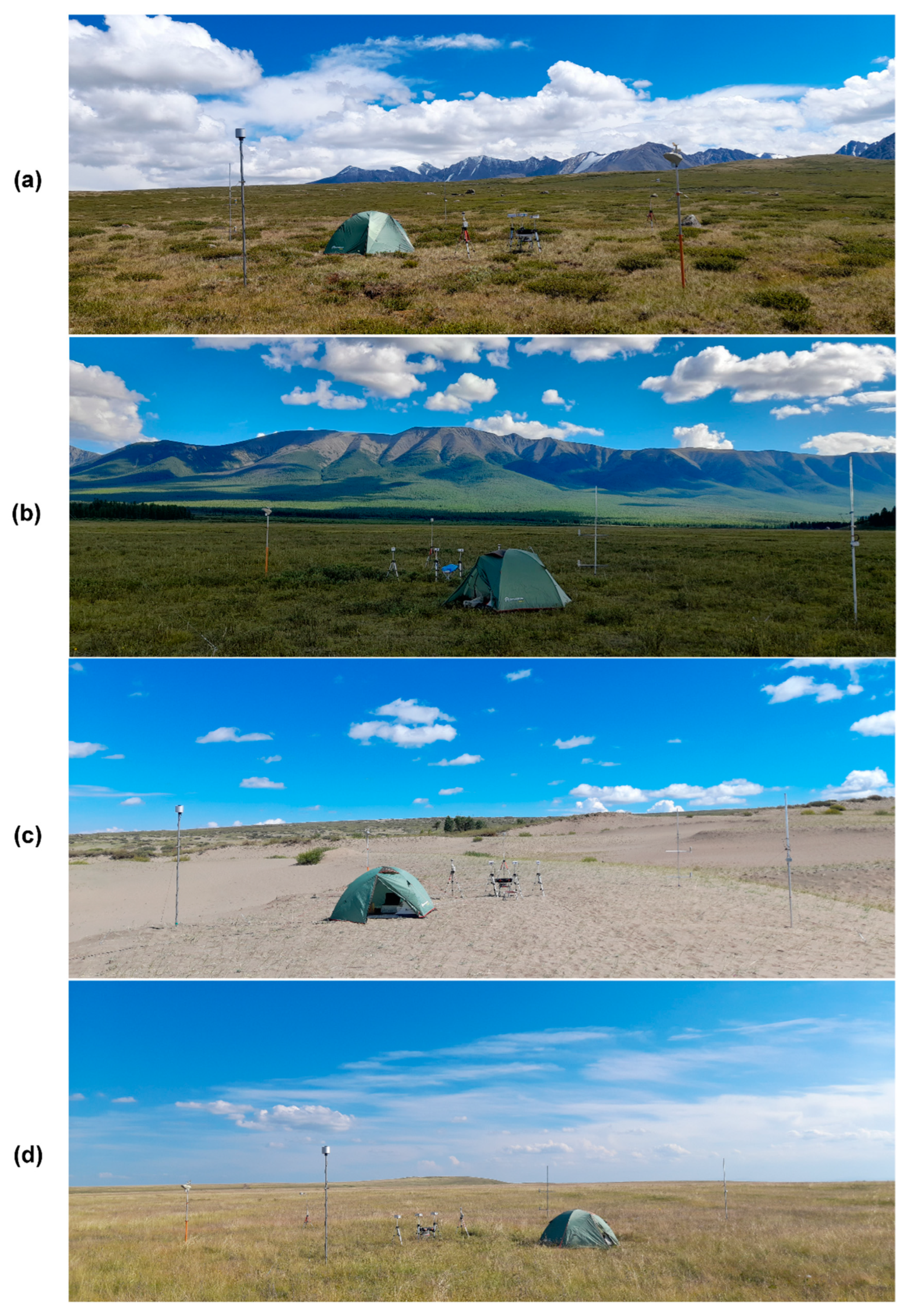
The measurements were carried out at four observation sites (Table 1, Figure 1b) at different altitudes above sea level and with different forms of landscape. Site 1 was located near Khindiktig-Khol lake and the Mongun-Taiga mountain massif, the landscape of which is mountainous tundra and alpine meadows (Figure A1). Point 2 was located in the Bayan-Tala tract, which is a steppe in the foothills of the Tannu-Ola ridge (Figure A2). Site 3 was located in the Shol tract, represented by a semi-desert landscape in the center of the Tyva depression (Figure A3). Site 4 was located in the Krasnaya Sopka tract between Belyo and Tus salt lakes in the Khakass-Minusinsk basin, represented by a steppe landscape (Figure A4).
For measurements at each of the observation sites, open homogeneous areas with a landscape characteristic of the area, not subject to anthropogenic impact, were selected. The location of the measuring equipment at each of the sites is shown in Figure A5.
At each of the sites, measurements were made under the conditions of an electrically undisturbed atmosphere of the main atmospheric-electrical and meteorological quantities, aerosol content, and gamma radiation background. In addition, video recording of the sky state and measurements of solar irradiance in the UV and visible ranges were carried out. Observations at each site ranged from 4 to 7 days (Table 1). In general, the obtained estimates can be considered representative for these territories and the season of the year. The only exception is the estimates of ion density variability at site 2, which are based on measurement data lasting less than a day (due to technical problems) and need to be refined.
2.2. Instruments
The positive (n+) and negative (n–) ion densities were measured with two air ion counters AIC2 (Alpha Lab, USA) [64]. This instrument is a true ion density meter, based on a Gerdien tube condenser design, and it contains a fan that draws air through the meter at a calibrated rate. A counter measures the number of positive or negative ions in air whose mobility is greater than 1 cm2∙V–1∙s–1. The maximum measurement of ion density is two million cm-3, the accuracy is about 20%. The counters were placed on tripods at a height of 1 m and measured the concentration of air ions with a time averaging of 1 s.
The electric field potential gradient (∇φ = –Ez = dφ/dz, where Ez and φ are the strength vertical component and potential of atmospheric electric field; the values under fair-weather conditions are positive) was measured using a portable electric field mill EFS-2/50 (NTCR, Russia). The field mill was preliminary calibrated using a calibration stand (plate capacitor) and brought to the readings of an electric field mill CS110 (Campbell Scientific, USA) [65] operating in monitoring mode at the geophysical observatory of IMCES SB RAS [66]. EFS-2/50 measures the potential gradient in the range of 0…±20 kV/m with an error of ±1%. The field mill was placed on a grounded tripod at a height of 2 m and measured with a time averaging of 1 s.
The main meteorological quantities (air temperature (t) and relative humidity (f), wind speed (V) and direction (D), atmospheric pressure, amount of precipitation, global solar radiation (SI), and UV index) were measured with 1-min averaging using an AW003 automatic weather station (Amtast, USA).
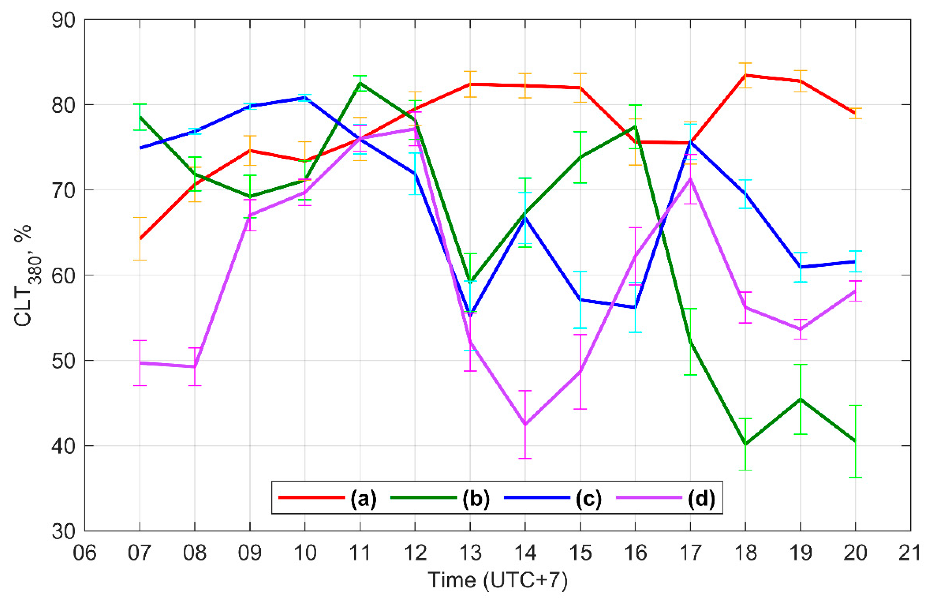
A NILU-UV-6T multichannel filter radiometer (Geminali, Norway) was used to measure solar radiation at 305, 312, 320, 340, and 380 nm and in the range of 400–700 nm, as well as to determine the average and maximum values of solar irradiance in the ranges of UV-A (315–400 nm), UV-B (280–315 nm), PAR (400–700 nm), erythemal and biologically active UV radiation, and also total ozone column, and transparency (CLT) of the atmosphere at 340 or 380 nm due to the cloud cover and aerosols. In our case, the CLT was calculated at 380 nm as
where Ee(meas.) and Ee(clear) are the measured and model (for a clear sky) irradiance at 380 nm.
Mass concentrations of particles with a diameter of less than 2.5 and 10 µm (PM2.5 and PM10) were measured using the SDS011 dust sensor (Shandong Nova Technology, China). SDS011 using the principle of light scattering measures the concentration of 0.3–10-µm particles in the air according to which concentrations of PM2.5 and PM10 values are calculated. The error in determining PM2.5 and PM10 is 20%.
The equivalent dose of gamma radiation (accumulation time of 3 h) was measured by a DT9501 radiation scanner (Shenzhen Everest Machinery Industry, China). DT9501 is a precision instrument that measures not only gamma, but alpha, beta, and X-ray radiation as well. The operation of the device is based on a Geiger-Muller counter converting ionizing radiation energy into electrical impulses and radiation dose.
Radon and its decay products were measured with a Ramon-02 radiometer (Solo LLP, Kazakhstan). The radiometer is a portable instrument measuring in semi-automatic mode the equivalent equilibrium volumetric activity of radon in the air in the range of 4−5·105 Bq/m3 with an error of ±30%.
2.3. Data Processing
The mathematical processing of measurement data included data sampling and statistical analysis. To interpret the variability and correlation of meteorological and geophysical quantities at different observation sites, the measurement data were synchronized. Then multi-day average hourly values were calculated. Using these data, statistical processing, correlation, and regression analyses of the daily variability of meteorological and geophysical quantities were carried out.
Also, the average hourly values of n± and ∇φ were used to calculate the conduction current density (Jλ) in the atmosphere using the formula [23]
where e is an elementary charge (1.6·10−19 C); k+ and k– are a mobility of positive and negative air ions which were taken equal to 1.2·10–4 V–1∙m–1∙s–2 [23].
3. Results
3.1. Variability and Diurnal Variation of n+
As seen in Figure 2 and Table B1, the average value of n+ at site 1 is 35·103 cm–3 (the median is 6.5·103 cm–3) and its typical range of variability, limited by the interval P25–P75, is (4–30)·103 cm–3. At site 2, the average value of n+ is 3.6·103 cm–3 (the median is 3.7·103 cm–3) and the typical range of variability is (3.0–4.2)·103 cm–3. At site 3, the average value of n+ is 23·103 cm–3 (the median is 3.7·103 cm–3) and, as a rule, varies in the range of (2.7–8.4)·103 cm–3. At site 4, the average value of n+ is 180·103 cm–3 (the median is 25·103 cm–3) and its typical range of variability corresponds to (4.3–51)·103 cm–3.
The probability distribution of n+ at sites 1–3 can be approximately described by a lognormal function (Figure 2). Moreover, at site 4, the distribution is bimodal.
According to Figure 3, the maximum values of n+ during the days are usually observed at night at 23-03 local time (LT), and the minimum – in the daytime at 10–19 LT. At the same time, during sunrise at 04–06 LT and after one at 05–08 LT, the secondary minimum and maximum were observed, respectively. At site 3, the secondary maximum n+ was comparable to the main one, and at site 4 it even exceeded it. In addition, at all observation sites in the afternoon at 15–17 LT, and at site 4 also in the evening at 19–21 LT, an increase of n+ was noted.
3.2. Variability and Diurnal Variation of n-
As seen in Figure 4 and Table B2, the average value of n– at site 1 is 0.6·103 cm–3 (the median is 0.3·103 cm–3) and its typical range of variability P25−P75 is limited in (0.1−0.9)·103 cm–3. At site 2, the average n– is 1.2·103 cm–3 (the median is 1.0·103 cm–3) and the typical range of variability is (0.8−1.5)·103 cm–3. At site 3, the average n– is 1.4·103 cm–3 (the median is 1.2·103 cm–3) and as a rule values vary in the range of (0.7−2.0)·103 cm–3. At site 4, the average value of n– is 1.0·103 cm–3 (the median is 0.7·103 cm–3) and its typical range of variability is (0.4−1.3)·103 cm–3.
The probability distribution of n– at sites 2 and 3 can be approximately described by a lognormal function (Figure 4). Moreover, at sites 1 and 4, the distribution, in general, is described by a power function and has a “heavy tail”.
According to Figure 5, in the daily variation of n– at observation sites, in general, increased values were noted at night and decreased values were observed during the day. However, in contrast to n+, the daily variations of n– at observation sites differ significantly from each other. Thus, at site 1, the maximum values of n– were observed in the periods of 23–02 LT, and the minimum values were observed at 17–20 LT. At the same time, the secondary maximum n– turned out to be higher than the main one. In point 3, the maximum values of n– were noted at 22–02 LT, and the minimum values at 11–16 LT. In addition, a secondary maximum was also observed at this site at 17–18 LT. At site 4, the maximum values of n– took place at 21–23 LT, the minimum values at 02 and 04 LT.
3.3. Variability and Diurnal Variation of ∇φ
As seen in Figure 6 and Table B3, the average value of ∇φ at site 1 is 120 V/m (the median is 110 V/m), and its typical range of variability limited by the interval P25−P75 is 100−130 V/m. At site 2, the average ∇φ is equal to 75 V/m (the median is 69 V/m) and the typical range of variability is 60−80 V/m. At site 3, the average value of ∇φ is 92 V/m (the median is 89 V/m) and, as a rule, one varies in the range of 80−110 V/m. At site 4, the average value of ∇φ is 77 V/m (the median is 68 V/m) and its typical range of variability corresponds to 50−90 V/m.
The probability distribution of ∇φ at all observation sites can be approximately described by the normal function (Figure 6). At the same time at site 4 an additional mode is superimposed on this distribution, the values of ∇φ in which are more than two times lower in the main mode.
According to Figure 7, at sites in the daily course ∇φ the main maximum is noted in the afternoon at 13–17 LT, and the main minimum is after midnight at 00‒01 LT. In addition, in the predawn hours at 03–04 LT and at sunrise at 05–07 LT, secondary maximum and minimum are observed, respectively. According to the classification [6,13,51], the observed diurnal variation of ∇φ can generally be attributed to the continental type with two maxima and two minima.
In addition to the observed maxima and minima, during the period at 09–12 LT with intense heating of the surface and boudary layer, a rapid increase in the potential gradient is observed, followed by stabilization or a slight decrease (“shoulder”), caused by a convective generator [3] (Figure 7).
At sites 2 and 4, during dawn and/or sunset, a significant increase of ∇φ was also observed (Figure 7). Moreover, at site 4, the value of ∇φ during these periods exceeded the main (afternoon) maximum. The cause of this effect is presumably the radiative cooling and formation of haze (fog) observed in anticyclonic conditions. Our assumption is confirmed by the daily variation of relative humidity at observation sites, the maximums of which, in general, are consistent with increasing the values of ∇φ. Due to orographic conditions and the relative proximity of water objects, increased air humidity is observed at these sites, which contributed to the formation of haze (fog). Thus, the average daily values of relative humidity at these sites were significantly (more than 10%) higher than the values at other sites.
Hourly average absolute and relative (% of the mean) values of the potential gradient under fair-weather conditions at observation sites are shown in Table C4.
3.4. Variability and Diurnal Variation of Jλ
The obtained values of Jλ at site 1 are in the range of (12‒130)·10−12 A/m2, the average is 70·10−12 A/m2, the median is 40·10−12 A/m2. Respectively, the values of Jλ at site 3 are (8‒43)·10−12 A/m2, 43·10−12 A/m2 и 11·10−12 A/m2, at site 4 are (12‒130)·10−12 A/m2, 70·10−12 A/m2 и 40·10−12 A/m2.
According to Figure 8, the daily variation of Jλ at observation sites, in general, resembles the daily variation of n+. The maximum values of Jλ are observed at night at 23–03 LT, and the minimum values are observed during the day at 10–19 LT. During sunrise at 04–06 LT and after sunrise at 05–08 LT, secondary minimum and maximum are observed, respectively. Moreover, at site 4, the secondary maximum Jλ exceeded the main maximum both in amplitude and in duration. The increasing of Jλ at site 4 in the afternoon at 15–17 LT and evening at 20–21 LT was also observed.
4. Discussion
The results of our studies of the daily cycle of small ions in the territory of Southern Siberia generally coincide with the results of similar studies conducted in other regions [67,68,69]. As in these works, the minimum ion concentrations we observed during the day and the increased concentrations in the evening, with a maximum at night, can be explained by the diurnal variability of radon concentrations and turbulent mixing during the day. These effects were reflected in the results of our observations. So, the observation sites 1 and 4 were located near relatively large lakes (Figs. A1 and A4) where breeze circulation was observed, when during the day the wind (an advective transport) was from the water surface to the land, and at night ‒ vice versa (Figs. E1j and E4j).
Since the main source of small ions on land is radon released from the soil, due to the transfer of “clean” air from the water area, where there is no radon emission, n+ and n− during this period in the surface layer will decrease. In addition, thermal turbulence, more intense in the daytime over land, enhances vertical mixing, which also leads to a “dilution” of the radon concentration in the surface layer and, accordingly, a decrease in the concentration of small ions. When southeastern advection from the mountain ridge at site 1 and western advection from the steppe at site 4 were observed, the ion concentration increased significantly.
As can be seen in Figure 3, the highest values of n+ were observed at site 4 in the steppe, located close (about 5 km) to salt lakes, which presumably can influence on n+. Also increased values of n+ in the daytime are observed at site 1 in the highlands near the Mongun-Taiga ridge. In general, there is a similarity in the daily variations of n+ at all observation sites. The Pearson correlation coefficient for sites 3 and 4 is 0.77, and for sites 1 and 3 it is 0.36 (Table С3). The highest values of n– are observed at site 3 in the Tyva depression, and the lowest values – at site 1 in the highlands. As can be seen in Figure 5, daily variations in n– at observation sites are weakly consistent with each other. The correlation for sites 1 and 3 is 0.35, for sites 1 and 4 – 0.30, and for sites 3 and 4 – 0.33 (Table C3).
A comparative analysis of the average values of ∇φ at observation sites showed the following. In general, the increase in the absolute altitude above sea level of observation sites coincides with an increase in the average (median) values of ∇φ. A similar relationship was previously noted in the Caucasus [19].
Based on the type of daily cycle of ∇φ, observation sites can be divided into two groups:
1) observation sites with a daily cycle for typical continental regions, having two maxima and two minima (sites 1 and 3);
2) sites with a more complex daily cycle due to the strong influence of local factors (sites 2 and 4).
The first group includes observation sites with a relatively dry climate, located in open, slightly winding terrain (the central part of the basin, a high mountain plateau). The second group, on the contrary, includes sites with a more humid climate, located in areas with complex terrain (mountain valley, shady slope of a mountain range), as well as near large bodies of water.
The obtained estimates of atmospheric-electrical quantities at observation sites, in general, are consistent with estimates of the characteristics of the radiation background at these sites. Thus, high values of n+ at sites 1 and 4 correspond to high values of γ-radiation dose (Figs. 2, 3, and D1). At sites 2 and 3, which are characterized by relatively low n+ values, the γ-radiation dose is also low. In this case, the distribution of average values of volumetric radon activity at observation sites is the inverse of γ-radiation dose and is in better agreement with the values of n− than with n+. The minimum values of radon volumetric activity, as well as n−, are noted at site 1, and the maximum at site 3 (Figs. 4, 5, and D2). A presumable explanation for the noted difference in the average values of volumetric radon activity at observation sites is the different permeability of the soils at the sites. The sandy soil at site 3 facilitates the emission of radon, and the rocky surface at site 1, on the contrary, hinders it. Based on the foregoing, the above-mentioned increase in average values of ∇φ with altitude can presumably be explained by a decrease in radon emission, which is associated with a change in the type of soil with an increase in the absolute altitude of the area. In the daily variation of γ-radiation dose and volumetric activity of radon, as well as in the daily variation of n+ and n−, the maximum, in general, occurs at night and early morning hours, and the minimum – in the daytime. Only the daily variation of the volumetric activity of radon at site 1 stands out from this dependence. This is presumably due to the weak emission of radon directly at this site and its transfer from adjacent territories. The daily variation of ∇φ, in general, is opposite to the daily variation of the above values, which is explained by the inverse relationship between the potential gradient and the electrical conductivity of the air, which is determined by n+ and n−.
There is also some consistency between atmospheric-electrical quantities, the aerosol content in the air, and the transparency of the atmosphere. The maximum values of PM2.5 and PM10 in the surface layer (at a height of 1 m) were recorded at site 4, which has the lowest altitude above sea level and is located on a steppe area near salt lakes, and the minimum values were recorded at site 1, located at a high mountain plateau (see Figure D3). Lower aerosol content was observed at site 2, located at the foot of the mountain range. Atmospheric transparency at a wavelength of 380 nm, on the contrary, was maximum at site 1 and minimum at site 4 (see Figure D4). At the same time, a direct relationship was noted between the absolute altitude of the sites and the average values of CLT380, which is most clearly manifested in the afternoon (13‒15 LT). Since the measurements were carried out mainly in clear and partly cloudy weather, the increase in CLT380 with altitude is mainly due to a decrease in the aerosol content with altitude. The latter should lead to a decrease in the electrical resistance of the atmosphere and an increase in the conduction current from the ionosphere to the Earth’s surface. The noted feature, in general, is consistent with the results obtained, according to which Jλ in the daytime increases with increasing absolute altitude of the area (see Figure D4).
Next, we will estimate the variability and relationship of hourly average values of atmospheric-electric quantities during the day with the main meteorological quantities (t, f, V, D), SI, CLT380, PM2.5 and equivalent dose of gamma radiation at each observation site. The average daily variations of these quantities are shown in Figure E1, Figure E2, Figure E3 and Figure E4, and the results of regression analysis are presented in Table F1, Table F2, Table F3 and Table F4.
Basically, at observation sites, the daily variability of n+, n− and ∇φ correlates with the variability of other measured quantities as moderate (R = 0.4‒0.6) and strong (R > 0.6). However, there is a weak relationship (R < 0.4) at some sites.
Thus, at site 1, the correlation between n− and ∇φ with PM2.5 is 0.33 and 0.30, respectively. At site 2, we observe a weak connection between ∇φ and V and D (0.45 and 0.42, respectively). At site 3, weak connections are noted between n+ and CLT380 (0.39), n− and t (0.49), n− and CLT380 (0.47), ∇φ and CLT380 (0.40). At site 4, the correlation is weak between n+ and SI (0.42), n+ and PM2.5 (0.32), n− and CLT380 (0.35), as well as between ∇φ and CLT380 (0.44), V (0.40) and D (0.37), f (0.33) and SI (0.32).
5. Conclusions
Using the field measuring data in the southern part of Siberia in the mountain-steppe landscapes of Khakassia and Tyva in July–August 2022, estimates of the general and daily variability of atmospheric electrical quantities under electrically undisturbed atmospheric conditions were obtained.
The maximum values of n+ were noted at the site in the Iyussko-Shirinsky steppe between Belyo and Tus salt lakes in the Khakass-Minusinsk basin. The maximum values of n– were observed at the site in the Shol tract in the center part of the Tyva depression.
The values of ∇φ tend to increase with altitude and reach a maximum in the highlands. The maximum values of ∇φ were noted in the highlands plateau near the Mongun-Taiga mountain massif and Khindiktig-Khol lake.
The maximum values of n+ during the day at observation sites are mainly observed at night (23–03 LT), and the minimum values are observed during the day at 10–19 LT. At 04–06 and 05–08 LT, a secondary minimum and maximum of n+ are observed, respectively. The daily cycles of n– are similar to n+, but differ from each other at different observation sites.
The main maximum of ∇φ is observed in the afternoon at 13-17 LT, and the main minimum ‒ after midnight at 00-01 LT. In addition to the main extremes of ∇φ, at 03–04 and 05–07 LT there are secondary maximums and minimums, respectively. An increase in humidity at dawn (sunset) led to an increase of ∇φ.
The diurnal cycles of ∇φ at different observation sites can be conditionally divided into two groups: 1) a diurnal cycle in the form of a double wave; 2) a daily cycle with a more complex course due to the strong influence of local factors.
The Jλ values at the observation sites varied in the range of 10−12 –10−9 A/m2, the maximum of Jλ in the daily variation, as a rule, was observed at night at 23–03 LT, the minimum during the day at 10–19 LT.
Author Contributions
Conceptualization, K.P.; methodology, K.P., P.N., M.O. and S.S.; software, K.P.; validation, K.P., P.N. and S.S.; formal analysis, K.P.; investigation, K.P.; resources, K.P., S.S., A.S. and M.O.; data curation, K.P., S.S., A.S. and M.O.; writing—original draft preparation, K.P. and M.O.; writing—review and editing, K.P., P.N., M.O. and S.S.; visualization, K.P.; supervision, K.P. and P.N.; project administration, K.P.; funding acquisition, K.P. All authors have read and agreed to the published version of the manuscript.
Funding
This research is supported by the Russian Science Foundation (Russia), project No.22-27-00482, https://www.rscf.ru/en/project/22-27-00482 (accessed on 1 August 2023).
Conflicts of Interest
The authors declare no conflict of interest.
Appendix A
Figure A1.
Location of site 1 (red star) on a plateau near the Mongun-Taiga mountain massif and Khindiktig-Khol lake.
Figure A1.
Location of site 1 (red star) on a plateau near the Mongun-Taiga mountain massif and Khindiktig-Khol lake.
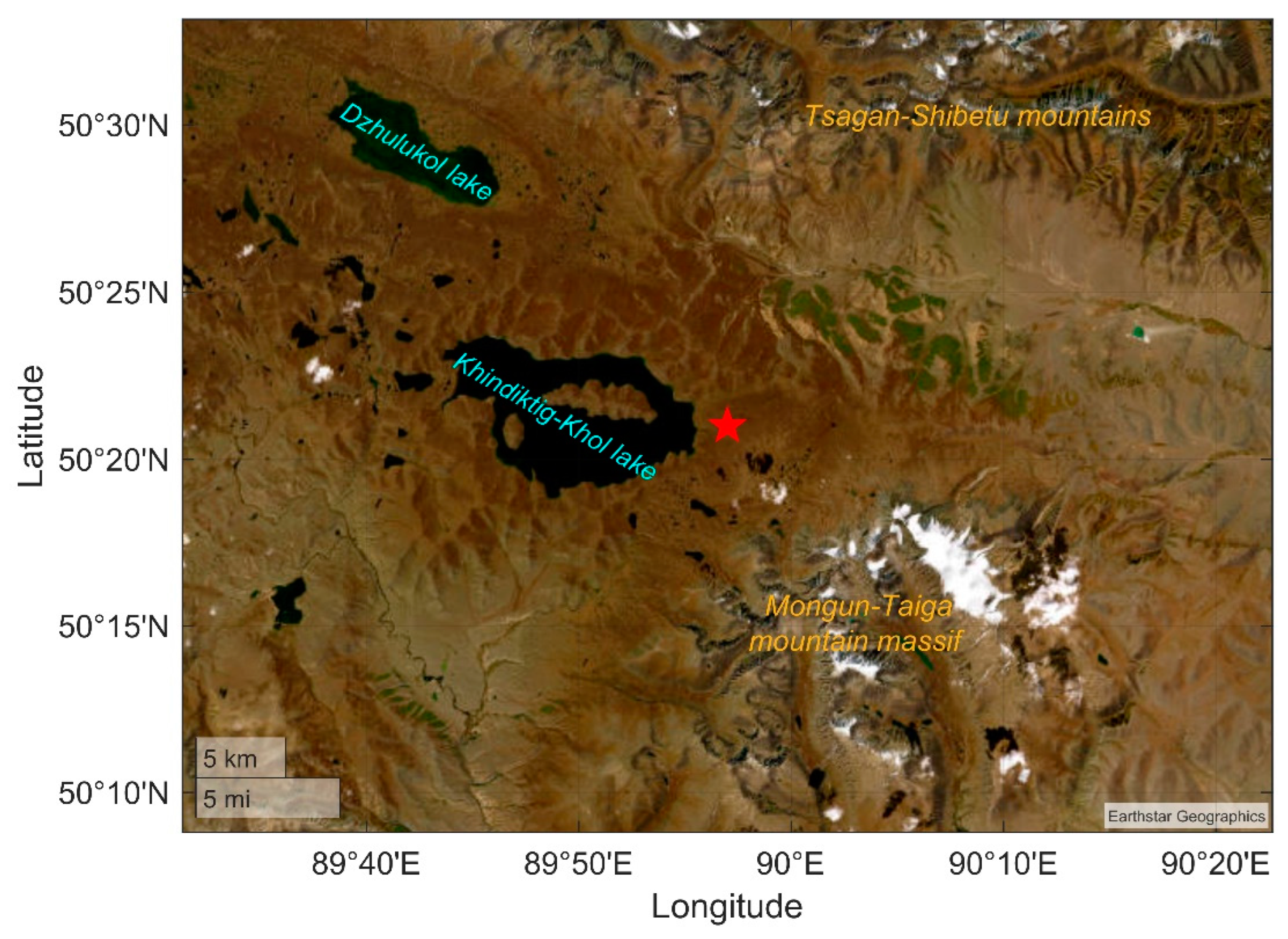
Figure A2.
Location of site 2 (red star) in the Bayan-Tala tract in the foothills of the Tannu-Ola ridge.
Figure A2.
Location of site 2 (red star) in the Bayan-Tala tract in the foothills of the Tannu-Ola ridge.
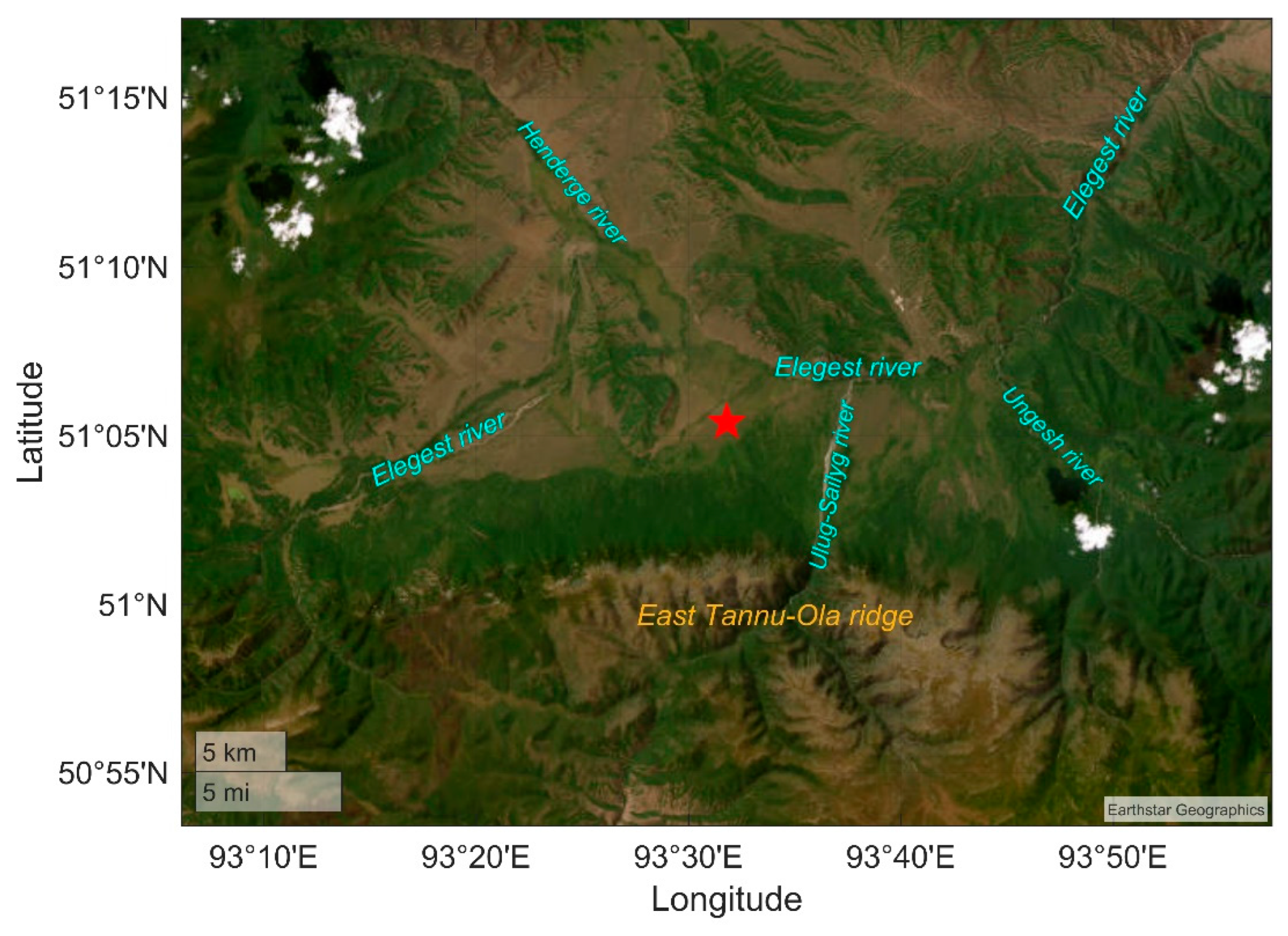
Figure A3.
Location of site 3 (red star) in the Shol tract in the center of the Tyva depression.
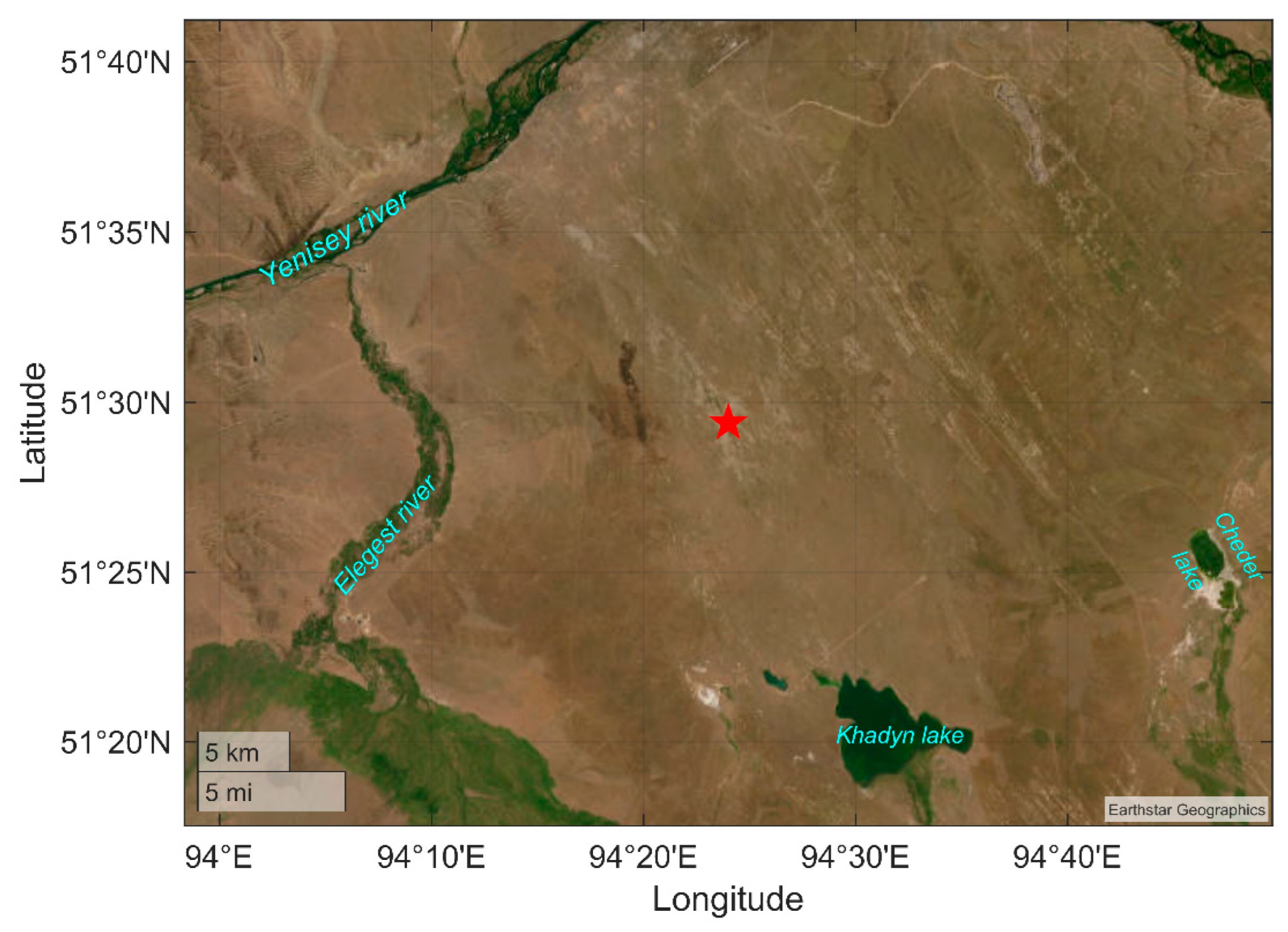
Figure A4.
Location of site 4 (red star) in the Krasnaya Sopka tract between Belyo and Tus salt lakes in the Khakass-Minusinsk basin.
Figure A4.
Location of site 4 (red star) in the Krasnaya Sopka tract between Belyo and Tus salt lakes in the Khakass-Minusinsk basin.
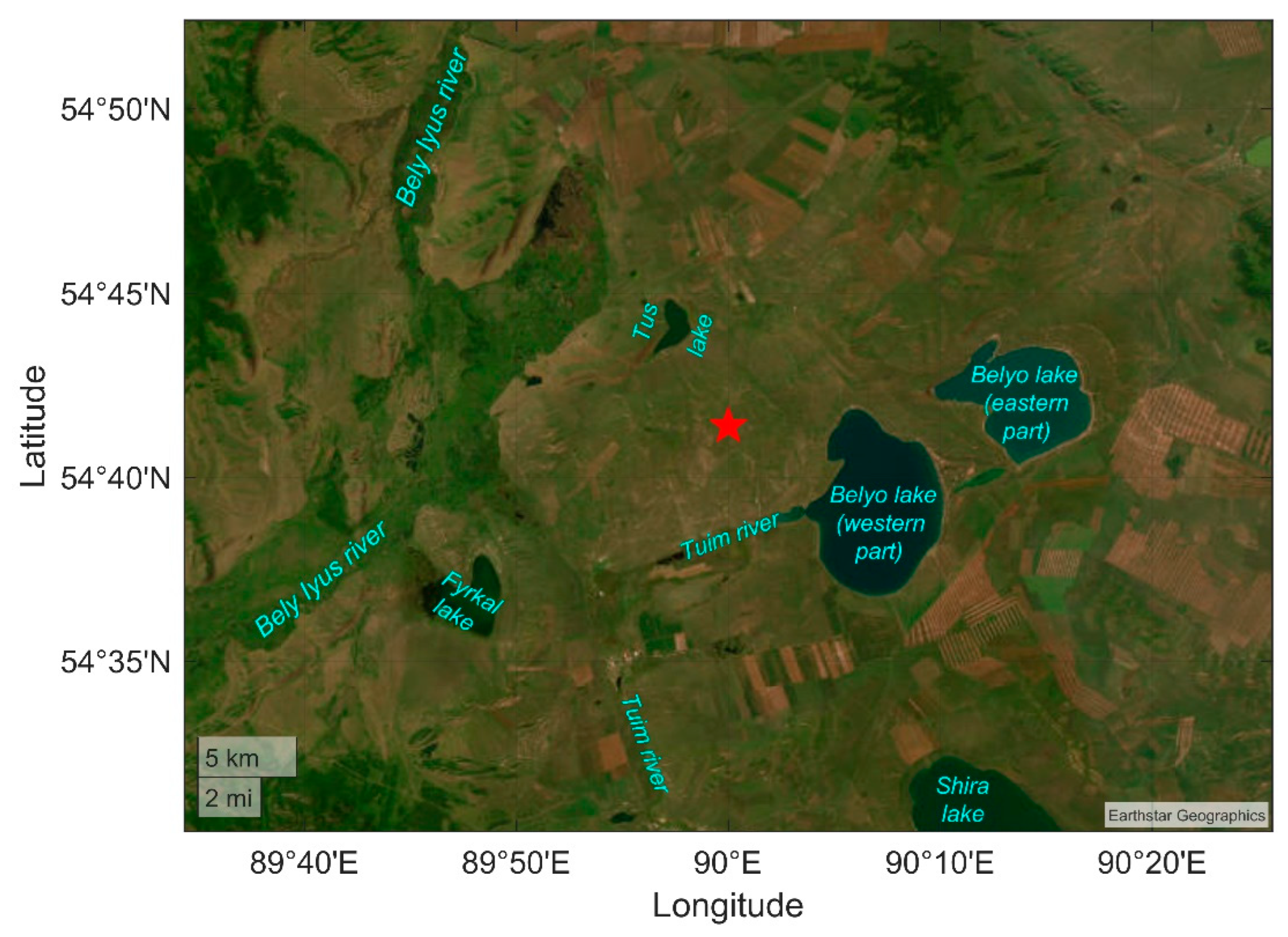
Figure A5.
Pictures of observation sites: 1 (a), 2 (b), 3 (c), and 4 (d).
Appendix B

Table B1.
Statistical parameters of the positive ion density variability under fair-weather conditions at observation sites.
Table B1.
Statistical parameters of the positive ion density variability under fair-weather conditions at observation sites.
| Site | Mean, 103 cm–3 | Standard Deviation, 103 cm–3 | Median, 103 cm–3 | Interquartile Range, 103 cm–3 | 5th Percentile, 103 cm–3 | 25th Percentile, 103 cm–3 | 75th Percentile, 103 cm–3 | 95th Percentile, 103 cm–3 |
|---|---|---|---|---|---|---|---|---|
| 1 | 35 | 78 | 6.5 | 26 | 3.0 | 4.4 | 30 | 200 |
| 2 * | 3.6 | 0.8 | 3.7 | 1.2 | 2.3 | 3.0 | 4.2 | 5.0 |
| 3 | 23 | 66 | 3.7 | 5.6 | 1.4 | 2.7 | 8.4 | 110 |
| 4 | 180 | 430 | 25 | 47 | 1.7 | 4.3 | 51 | 1400 |
Table B2.
Statistical parameters of the negative ion density variability under fair-weather conditions at observation sites.
Table B2.
Statistical parameters of the negative ion density variability under fair-weather conditions at observation sites.
| Site | Mean, 103 cm–3 | Standard Deviation, 103 cm–3 | Median, 103 cm–3 | Interquartile Range, 103 cm–3 | 5th Percentile, 103 cm–3 | 25th Percentile, 103 cm–3 | 75th Percentile, 103 cm–3 | 95th Percentile, 103 cm–3 |
|---|---|---|---|---|---|---|---|---|
| 1 | 0.6 | 0.6 | 0.3 | 0.8 | 0.04 | 0.1 | 0.9 | 1.9 |
| 2 * | 1.2 | 0.6 | 1.0 | 0.7 | 0.6 | 0.8 | 1.5 | 2.5 |
| 3 | 1.4 | 0.5 | 1.2 | 1.3 | 0.3 | 0.7 | 2.0 | 3.1 |
| 4 | 1.0 | 0.9 | 0.7 | 0.9 | 0.2 | 0.4 | 1.3 | 3.1 |
Table B3.
Statistical parameters of the electric field potential gradient variability under fair-weather conditions at observation sites.
Table B3.
Statistical parameters of the electric field potential gradient variability under fair-weather conditions at observation sites.
| Site | Mean, V/m | Standard Deviation, V/m | Median, V/m | Interquartile Range, V/m | 5th Percentile, V/m | 25th Percentile, V/m | 75th Percentile, V/m | 95th Percentile, V/m |
|---|---|---|---|---|---|---|---|---|
| 1 | 120 | 31 | 110 | 33 | 77 | 96 | 130 | 160 |
| 2 | 75 | 38 | 69 | 26 | 42 | 57 | 83 | 120 |
| 3 | 92 | 28 | 89 | 29 | 52 | 76 | 110 | 140 |
| 4 | 77 | 48 | 68 | 38 | 25 | 51 | 89 | 150 |
Table B4.
Statistical parameters of the conduction current density variability under fair-weather conditions at observation sites.
Table B4.
Statistical parameters of the conduction current density variability under fair-weather conditions at observation sites.
| Site | Mean, 10−12 A/m2 | Standard Deviation, 10−12 A/m2 | Median, 10−12 A/m2 | Interquartile Range, 10−12 A/m2 | 5th Percentile, 10−12 A/m2 | 25th Percentile, 10−12 A/m2 | 75th Percentile, 10−12 A/m2 | 95th Percentile, 10−12 A/m2 |
|---|---|---|---|---|---|---|---|---|
| 1 | 70 | 80 | 40 | 120 | 10 | 12 | 130 | 230 |
| 2 * | − | − | − | − | − | − | − | − |
| 3 | 43 | 63 | 11 | 38 | 7 | 8 | 46 | 190 |
| 4 | 350 | 680 | 30 | 360 | 8 | 14 | 380 | 2100 |
Appendix C
Table C1.
Regression equations and coefficients of determination (R2) for the hourly average positive ion density (cm-3) at observation sites.
Table C1.
Regression equations and coefficients of determination (R2) for the hourly average positive ion density (cm-3) at observation sites.
| Predictor | Site 1 | Site 2 * | Site 3 | Site 4 |
|---|---|---|---|---|
| Site 1 | – | Y = –7.90·10–2·X + 4.31·103 R2 = 0.41 |
Y = 3.81·10–1·X + 1.31·104 R2 = 0.13 |
Y = 1.43·X + 1.55·105 R2 = 0.02 |
| Site 2 * | Y = –5.22·X + 2.75·104 R2 = 0.41 |
– | Y = –2.62·10–1·X + 4.12·103 R2 = 0.23 |
Y = –9.42·X + 6.46·104 R2 = 0.17 |
| Site 3 | Y = 3.46·10–1·X + 2.62·104 R2 = 0.13 |
Y = –8.66·10–1·X + 6.38·103 R2 = 0.23 |
– | Y = 6.76·X + 2.59·104 R2 = 0.59 |
| Site 4 | Y = 1.69·10–2·X + 3.2·104 R2 = 0.02 |
Y = –1.79·10–2·X + 4.17·103 R2 = 0.17 |
Y = 8.76·10–1·X + 8.57·103 R2 = 0.59 |
– |
Table C2.
Regression equations and coefficients of determination (R2) for the hourly average negative ion density (cm-3) at observation sites.
Table C2.
Regression equations and coefficients of determination (R2) for the hourly average negative ion density (cm-3) at observation sites.
| Predictor | Site 1 | Site 2 * | Site 3 | Site 4 |
|---|---|---|---|---|
| Site 1 | – | Y = –2.44·10–1·X + 1.15·103 R2 = 0.02 |
Y = 2.96·10–1·X + 1.28·103 R2 = 0.12 |
Y = –2.46·10–1·X + 1.11·103 R2 = 0.09 |
| Site 2 * | Y = –8.63·10–2·X + 2.71·102 R2 = 0.02 |
– | Y = –2.66·10–1·X + 1.82·103 R2 = 0.05 |
Y = 2.56·10–1·X + 9.35·102 R2 = 0.04 |
| Site 3 | Y = 4.12·10–1·X + 1.31·101 R2 = 0.12 |
Y = –1.97·10–1·X + 1.41·103 R2 = 0.05 |
– | Y = 3.25·10–1·X + 4.82·102 R2 = 0.11 |
| Site 4 | Y = –3.55·10–1·X + 9.56·102 R2 = 0.09 |
Y = 1.36·10–1·X + 9.40·102 R2 = 0.04 |
Y = 3.38·10–1·X + 1.14·103 R2 = 0.11 |
– |
Table C3.
Regression equations and coefficients of determination (R2) for the hourly average potential gradient (V/m) at observation sites.
Table C3.
Regression equations and coefficients of determination (R2) for the hourly average potential gradient (V/m) at observation sites.
| Predictor | Site 1 | Site 2 | Site 3 | Site 4 |
|---|---|---|---|---|
| Site 1 | – | Y = 2.58·10–1·X + 4.51·101 R2 = 0.04 |
Y = 8.36·10–1·X – 4.27·100 R2 = 0.51 |
Y = –1.56·10–1·X + 9.53·101 R2 = 0.01 |
| Site 2 | Y = 1.72·10–1·X + 1.02·102 R2 = 0.04 |
– | Y = 4.79·10–1·X + 5.61·101 R2 = 0.25 |
Y = 7.51·10–1·X + 2.12·101 R2 = 0.23 |
| Site 3 | Y = 6.07·10–1·X + 5.93·101 R2 = 0.51 |
Y = 5.21·10–1·X + 2.69·101 R2 = 0.25 |
– | Y = 5.98·10–1·X + 2.24·101 R2 = 0.13 |
| Site 4 | Y = –4.22·10–2·X + 1.18·102 R2 = 0.01 |
Y = 3.04·10–1·X + 5.13·101 R2 = 0.23 |
Y = 2.22·10–1·X + 7.47·101 R2 = 0.13 |
– |
Table C4.
Hourly average absolute (V/m) and relative (% of the mean) values of potential gradient under fair-weather conditions at observation sites.
Table C4.
Hourly average absolute (V/m) and relative (% of the mean) values of potential gradient under fair-weather conditions at observation sites.
| Time (UTC/LT) | Site 1 | Site 2 | Site 3 | Site 4 | ||||
|---|---|---|---|---|---|---|---|---|
| V/m | % of mean | V/m | % of mean | V/m | % of mean | V/m | % of mean | |
| 00/07 | 94 | 82 | 100 | 133 | 88 | 96 | 153 | 199 |
| 01/08 | 108 | 94 | 80 | 107 | 98 | 107 | 132 | 171 |
| 02/09 | 117 | 102 | 72 | 96 | 113 | 123 | 100 | 130 |
| 03/10 | 111 | 97 | 73 | 97 | 106 | 115 | 83 | 108 |
| 04/10 | 121 | 105 | 85 | 113 | 105 | 114 | 76 | 99 |
| 05/11 | 117 | 102 | 93 | 124 | 105 | 114 | 89 | 116 |
| 06/12 | 120 | 104 | 113 | 151 | 110 | 120 | 93 | 121 |
| 07/13 | 122 | 106 | 80 | 107 | 104 | 113 | 107 | 139 |
| 08/14 | 130 | 113 | 76 | 101 | 108 | 117 | 78 | 101 |
| 09/15 | 138 | 120 | 86 | 115 | 105 | 114 | 78 | 101 |
| 10/17 | 141 | 123 | 76 | 101 | 113 | 123 | 65 | 84 |
| 11/18 | 133 | 116 | 70 | 93 | 106 | 115 | 65 | 84 |
| 12/19 | 124 | 108 | 63 | 84 | 90 | 98 | 52 | 68 |
| 13/20 | 115 | 100 | 108 | 144 | 86 | 93 | 49 | 64 |
| 14/21 | 115 | 100 | 63 | 84 | 89 | 97 | 47 | 61 |
| 15/22 | 112 | 97 | 61 | 81 | 86 | 93 | 50 | 65 |
| 16/23 | 94 | 82 | 62 | 83 | 64 | 70 | 55 | 71 |
| 17/00 | 85 | 74 | 55 | 73 | 66 | 72 | 48 | 62 |
| 18/01 | 102 | 89 | 54 | 72 | 70 | 76 | 66 | 86 |
| 19/02 | 102 | 89 | 60 | 80 | 77 | 84 | 67 | 87 |
| 20/03 | 115 | 100 | 65 | 87 | 93 | 101 | 80 | 104 |
| 21/04 | 122 | 106 | 58 | 77 | 82 | 89 | 82 | 106 |
| 22/05 | 114 | 99 | 55 | 73 | 69 | 75 | 62 | 81 |
| 23/06 | 108 | 94 | 83 | 111 | 71 | 77 | 79 | 103 |
Appendix D
Figure D1.
Average equivalent dose of gamma radiation for the 6-h periods (01−07, 07−13, 13−19, and 19−01 LT) under fair-weather conditions at observation sites: 1 (a), 2 (b), 3 (c), and 4 (d).
Figure D1.
Average equivalent dose of gamma radiation for the 6-h periods (01−07, 07−13, 13−19, and 19−01 LT) under fair-weather conditions at observation sites: 1 (a), 2 (b), 3 (c), and 4 (d).
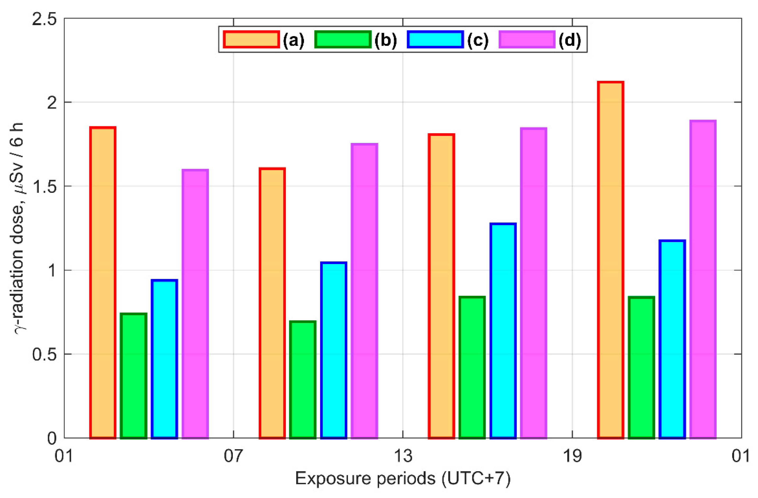
Figure D2.
Average equivalent equilibrium volumetric activity of radon at 01, 07, 13, and 19 LT under fair-weather conditions at observation sites: 1 (a), 3 (b), and 4 (c).
Figure D2.
Average equivalent equilibrium volumetric activity of radon at 01, 07, 13, and 19 LT under fair-weather conditions at observation sites: 1 (a), 3 (b), and 4 (c).
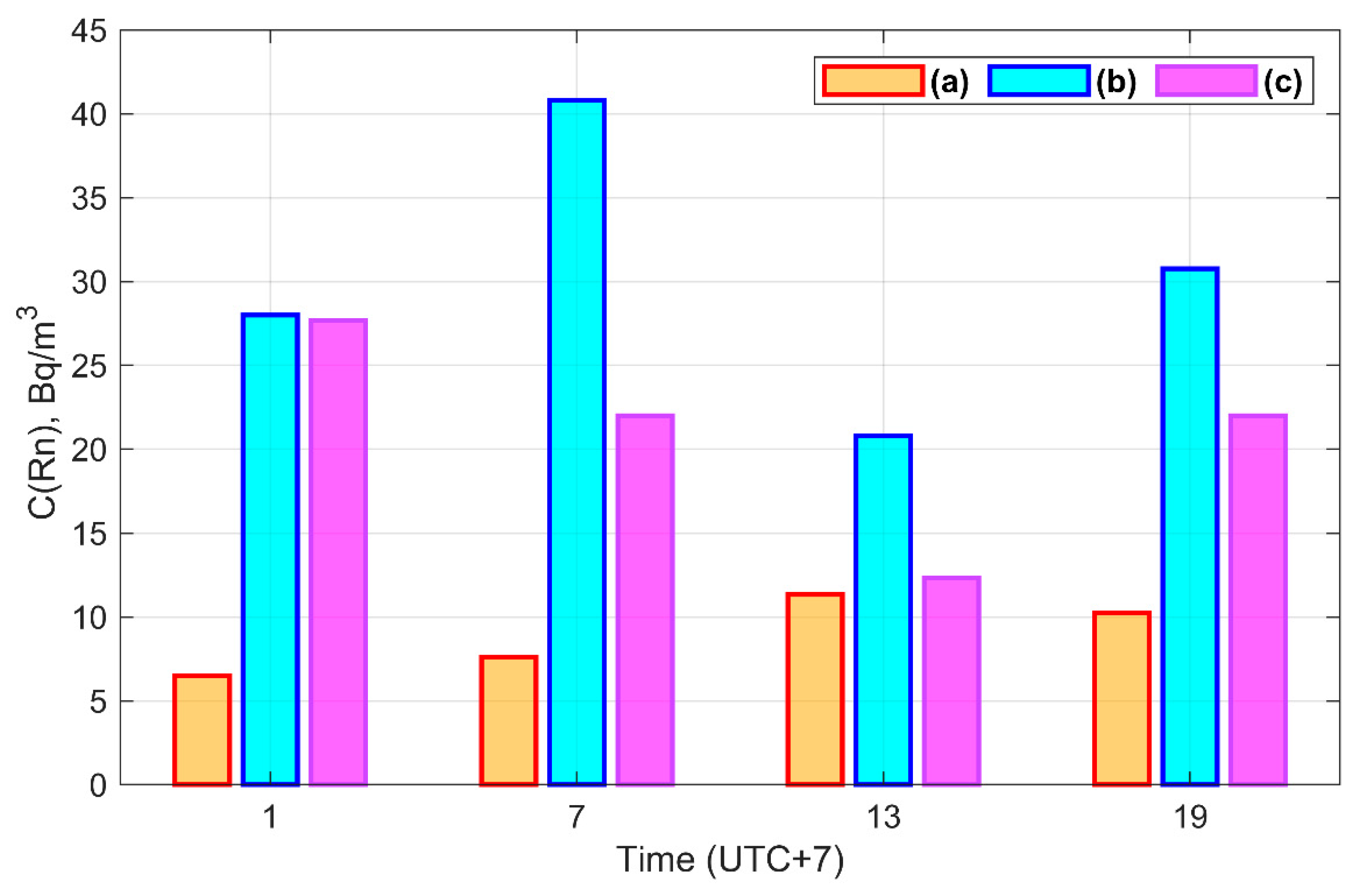
Figure D3.
Hourly average PM2.5 variations under fair-weather conditions at observation sites: 1 (a), 3 (b), and 4 (c).
Figure D3.
Hourly average PM2.5 variations under fair-weather conditions at observation sites: 1 (a), 3 (b), and 4 (c).
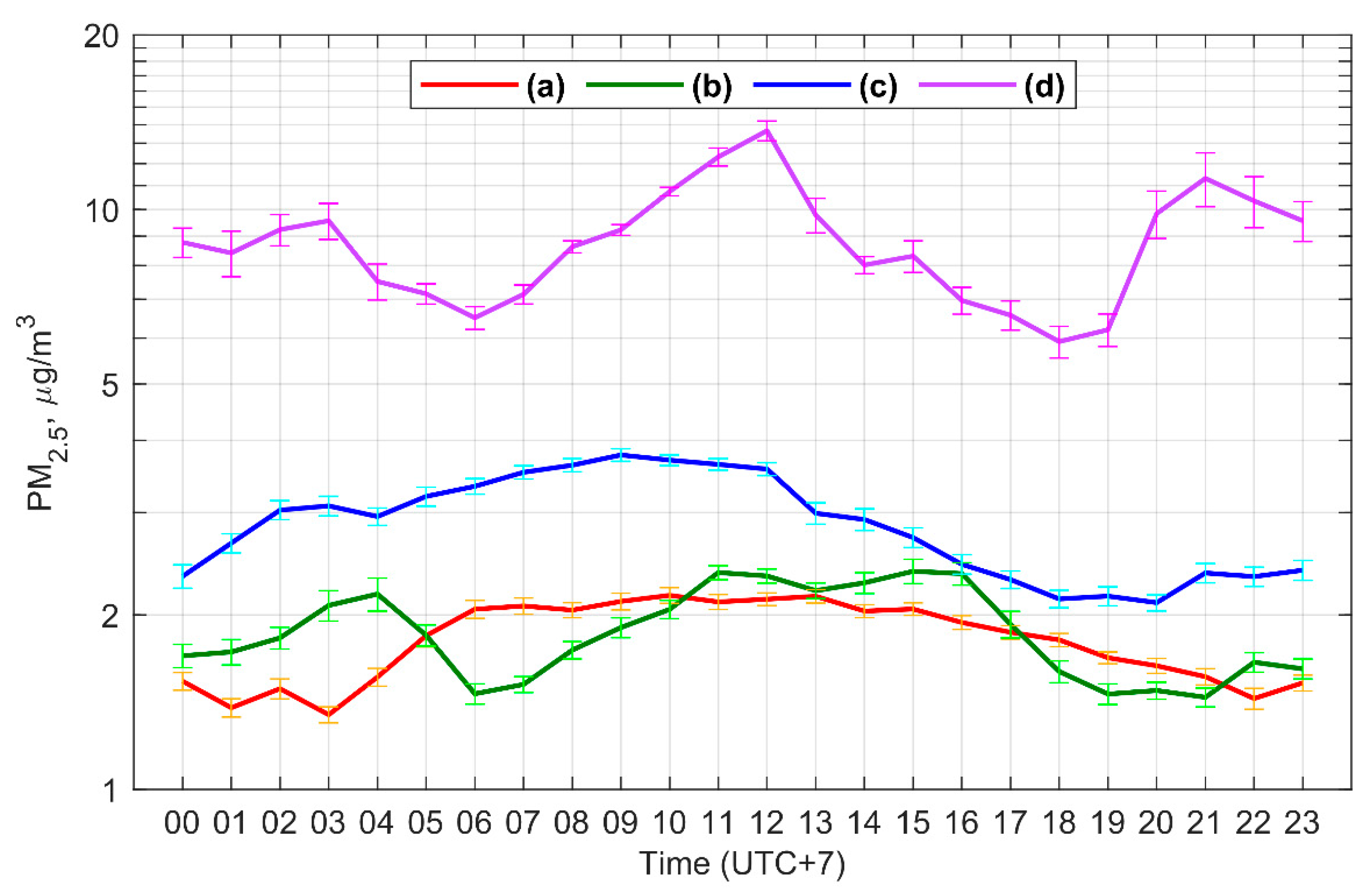
Figure D4.
Hourly average CLT380 variations under fair-weather conditions at observation sites: 1 (a), 3 (b), and 4 (c).
Figure D4.
Hourly average CLT380 variations under fair-weather conditions at observation sites: 1 (a), 3 (b), and 4 (c).
Appendix E
Figure E1.
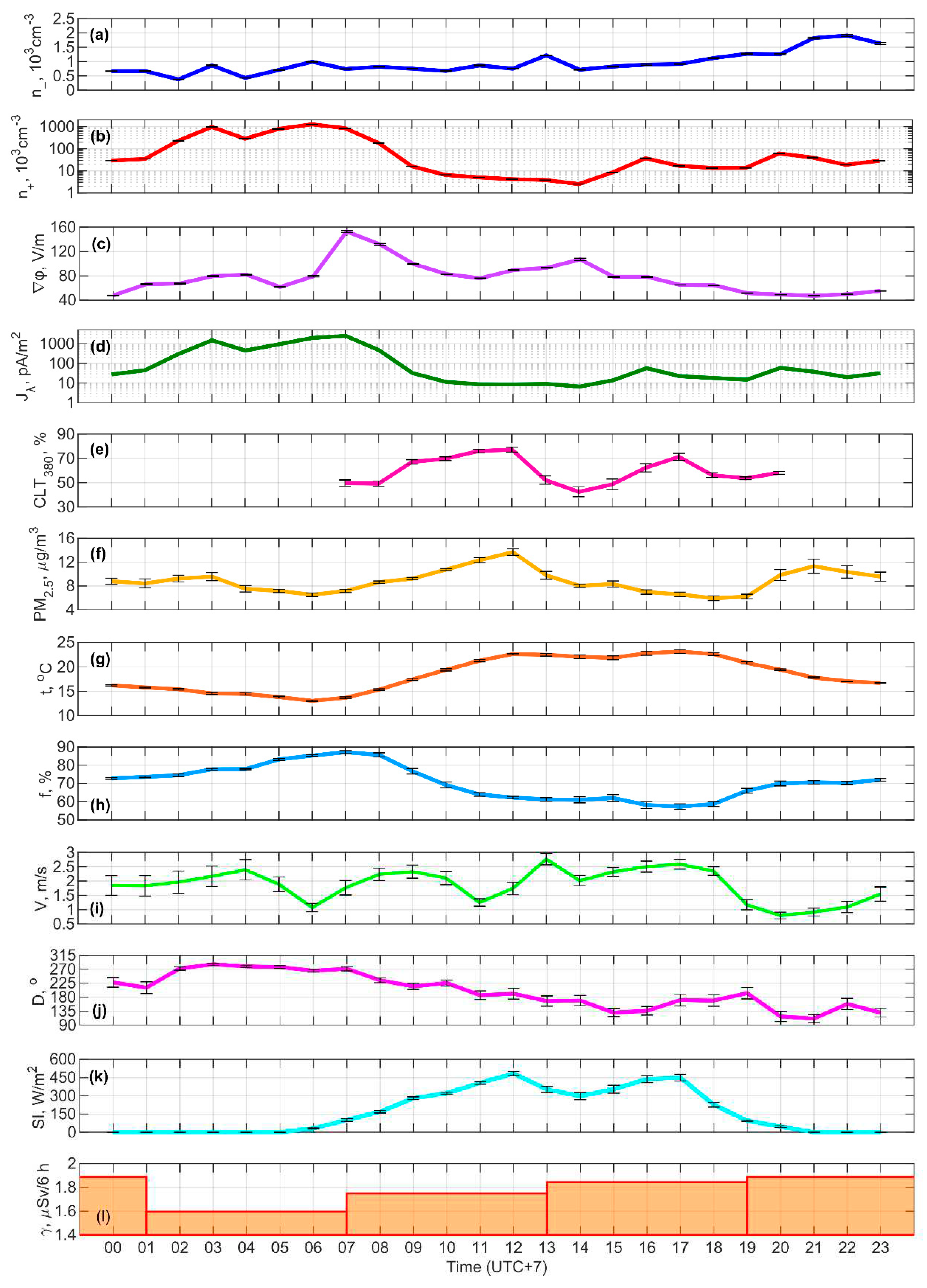
Hourly average variations of negative (a) and positive (b) ion densities, potential gradient (c), conduction current density (d), atmospheric transparency at 380 nm (e), mass concentration of PM2.5 (f), air temperature (g), air relative humidity (h), wind speed (i) and direction (j), global solar radiation (k), and equivalent dose of gamma radiation (l) under fair-weather conditions at site 1.
Figure E1.
Hourly average variations of negative (a) and positive (b) ion densities, potential gradient (c), conduction current density (d), atmospheric transparency at 380 nm (e), mass concentration of PM2.5 (f), air temperature (g), air relative humidity (h), wind speed (i) and direction (j), global solar radiation (k), and equivalent dose of gamma radiation (l) under fair-weather conditions at site 1.
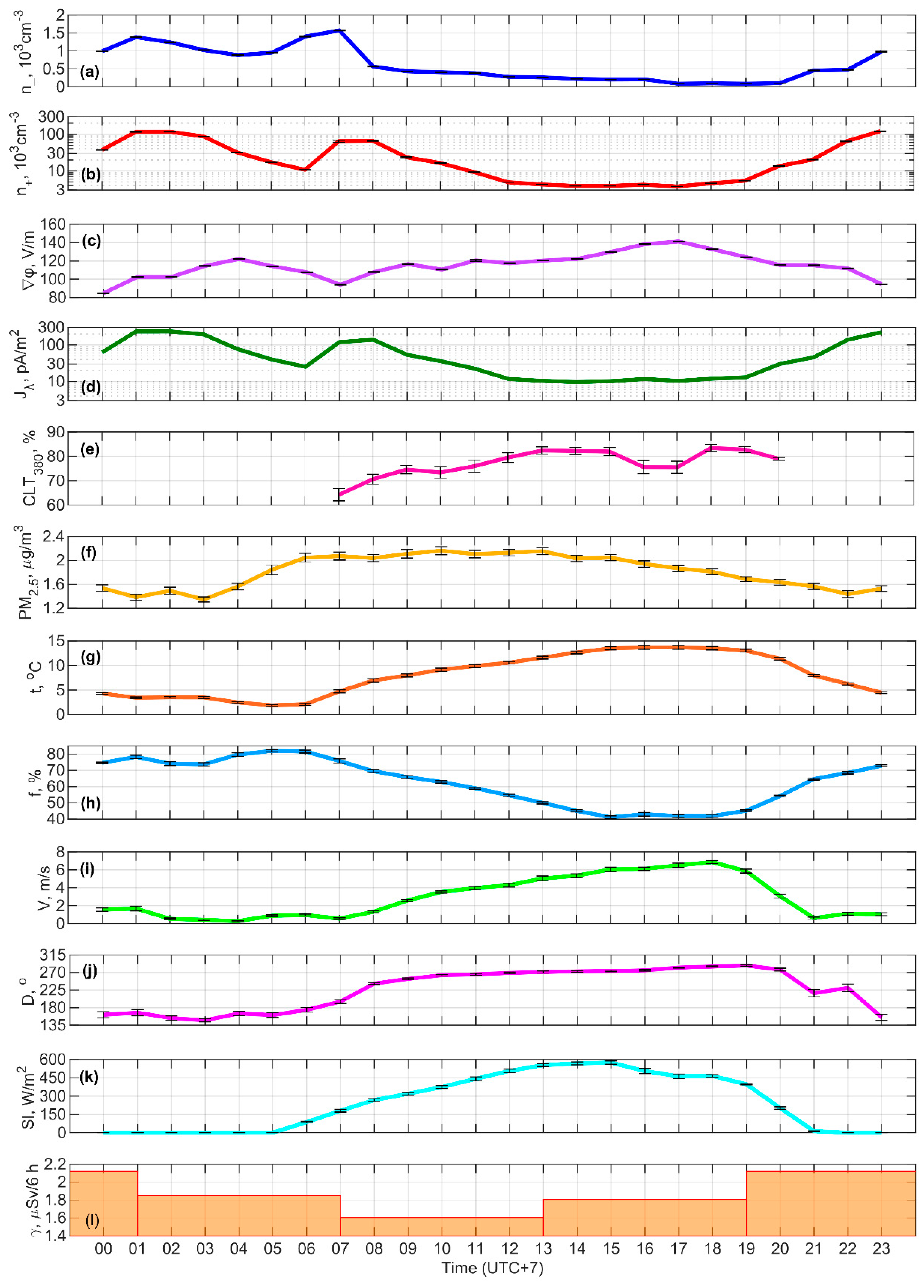
Figure E2.
Hourly average variations of negative (a) and positive (b) ion densities, potential gradient (c), conduction current density (d), atmospheric transparency at 380 nm (e), mass concentration of PM2.5 (f), air temperature (g), air relative humidity (h), wind speed (i) and direction (j), global solar radiation (k), and equivalent dose of gamma radiation (l) under fair-weather conditions at site 2.
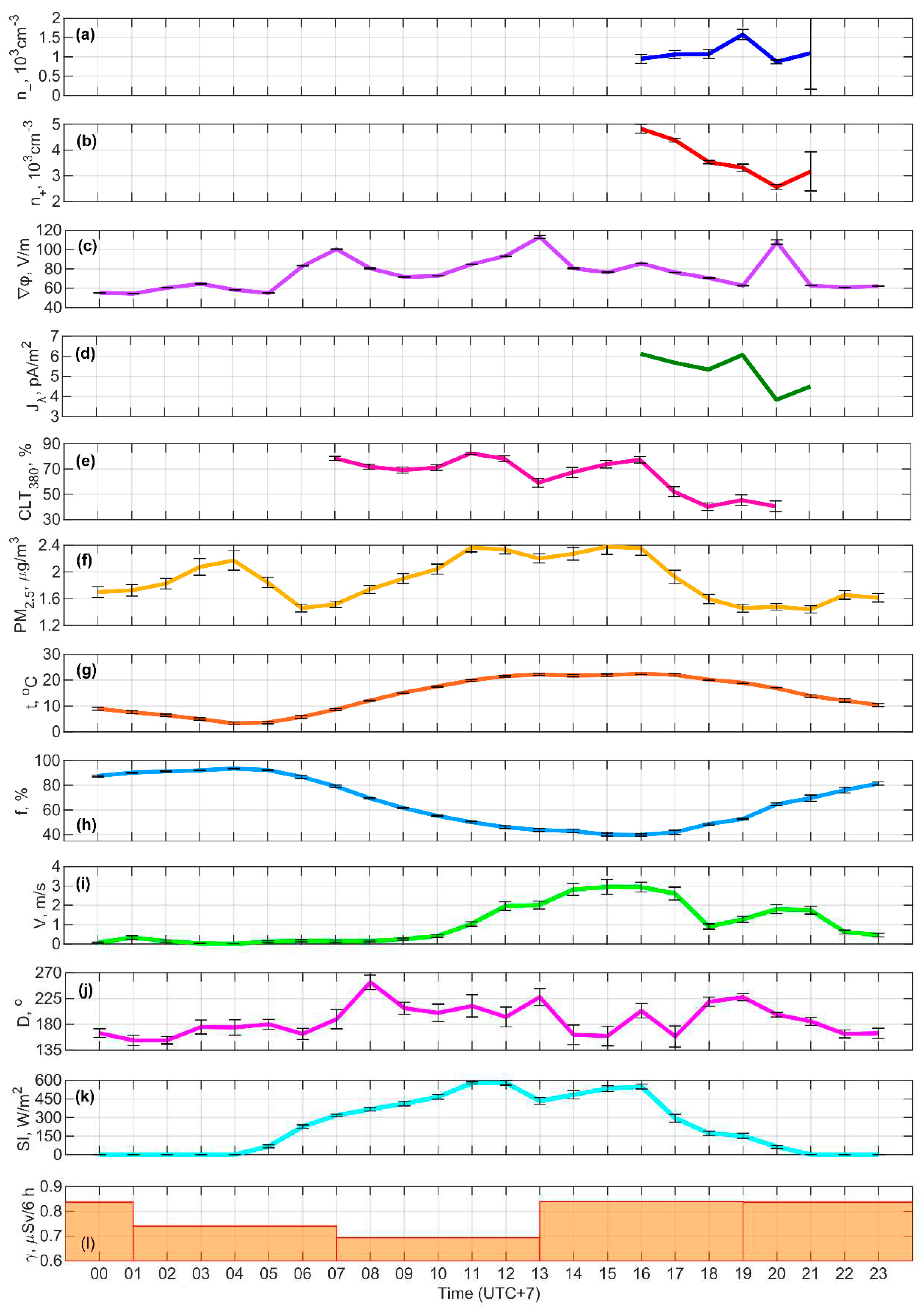
Figure E3.
Hourly average variations of negative (a) and positive (b) ion densities, potential gradient (c), conduction current density (d), atmospheric transparency at 380 nm (e), mass concentration of PM2.5 (f), air temperature (g), air relative humidity (h), wind speed (i) and direction (j), global solar radiation (k), and equivalent dose of gamma radiation (l) under fair-weather conditions at site 3.
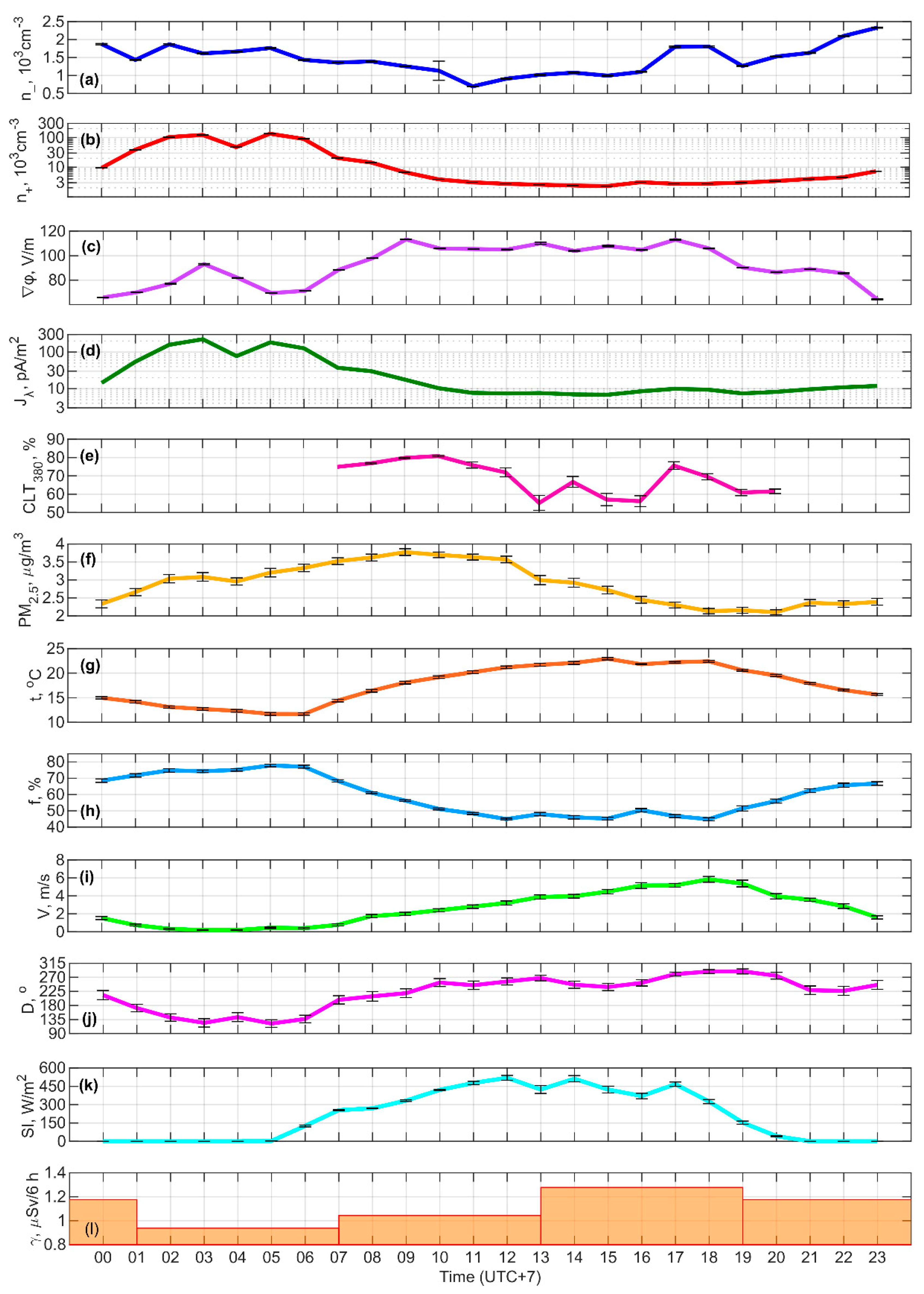
Figure E4.
Hourly average variations of negative (a) and positive (b) ion densities, potential gradient (c), conduction current density (d), atmospheric transparency at 380 nm (e), mass concentration of PM2.5 (f), air temperature (g), air relative humidity (h), wind speed (i) and direction (j), global solar radiation (k), and equivalent dose of gamma radiation (l) under fair-weather conditions at site 4.
Appendix F
Table F1.
Regression equations and coefficients of determination (R2) for the hourly average quantities measured at site 1.
Table F1.
Regression equations and coefficients of determination (R2) for the hourly average quantities measured at site 1.
| Predictor | n+, cm-3 | n–, cm-3 | ∇φ, V/m |
|---|---|---|---|
| n+, cm-3 | – | Y = 8.15·10–3·X + 3.27·102 R2 = 0.47 |
Y = – 2.21·10–1·X + 1.23·102 R2 = 0.42 |
| n–, cm-3 | Y = 5.75·101·X + 2.06·101 R2 = 0.47 |
– | Y = –2.14·10–2·X + 1.28·102 R2 = 0.56 |
| ∇φ, V/m | Y = –1.89·103·X + 2.53·105 R2 = 0.42 |
Y = –2.59·101·X + 3.6·103 R2 = 0.56 |
– |
| CLT380, % | Y = –3.24·103·X + 2.66·105 R2 = 0.68 |
Y = –5.74·101·X + 4.78·103 R2 = 0.68 |
Y = 1.39·X + 1.36·101 R2 = 0.38 |
| PM2.5, µg/m3 | Y = –8.87·104·X + 1.96·105 R2 = 0.39 |
Y = –5.61·102·X + 1.63·103 R2 = 0.11 |
Y = 1.44·101·X + 8.88·101 R2 = 0.09 |
| t, °C | Y = –6.07·103·X + 8.41·104 R2 = 0.42 |
Y = –1.00·102·X + 1.42·103 R2 = 0.80 |
Y = 2.34·X + 9.63·101 R2 = 0.53 |
| f, % | Y = 1.73·103·X – 7.24·104 R2 = 0.38 |
Y = 2.90·101·X – 1.2·103 R2 = 0.76 |
Y = –7.24·10–1·X + 1.60·102 R2 = 0.58 |
| V, m/s | Y = –1.13·104·X + 6.85·104 R2 = 0.43 |
Y = –1.63·102·X + 1.09·103 R2 = 0.63 |
Y = 4.42·X + 1.02·102 R2 = 0.56 |
| D, ° | Y = –5.38·102·X + 1.58·105 R2 = 0.51 |
Y = –8.03·X + 2.44·103 R2 = 0.80 |
Y = 1.79·10–1·X + 7.45·101 R2 = 0.48 |
| SI, W/m2 | Y = –1.19·102·X + 6.47·104 R2 = 0.46 |
Y = –1.53·X + 9.94·102 R2 = 0.55 |
Y = 3.99·10–2·X + 1.05·102 R2 = 0.45 |
Table F2.
Regression equations and coefficients of determination (R2) for the hourly average quantities measured at site 2.
Table F2.
Regression equations and coefficients of determination (R2) for the hourly average quantities measured at site 2.
| Predictor | n+, cm-3* | n–, cm-3* | ∇φ, V/m |
|---|---|---|---|
| n+, cm-3* | – | – | – |
| n–, cm-3* | – | – | – |
| ∇φ, V/m | – | – | – |
| CLT380, % | – | – | Y = 9.22·10–2·X + 7.81·101 R2 = 0.01 |
| PM2.5, µg/m3 | – | – | Y = 1.08·101·X + 5.45·101 R2 = 0.05 |
| t, °C | – | – | Y = 1.29·X + 5.66·101 R2 = 0.27 |
| f, % | – | – | Y = –4.46·10–1·X + 1.04·102 R2 = 0.28 |
| V, m/s | – | – | Y = 7.15·X + 6.73·101 R2 = 0.20 |
| D, ° | – | – | Y = 2.55·10–1·X + 2.71·101 R2 = 0.18 |
| SI, W/m2 | – | – | Y = 4.50·10–1·X + 6.40·101 R2 = 0.36 |
Table F3.
Regression equations and coefficients of determination (R2) for the hourly average quantities measured at site 3.
Table F3.
Regression equations and coefficients of determination (R2) for the hourly average quantities measured at site 3.
| Predictor | n+, cm-3 | n–, cm-3 | ∇φ, V/m |
|---|---|---|---|
| n+, cm-3 | – | Y = 2.75·10–3·X + 1.39·103 R2 = 0.08 |
Y = –1.90·10–4·X + 9.69·101 R2 = 0.25 |
| n–, cm-3 | Y = 2.97·101·X – 1.69·104 R2 = 0.08 |
– | Y = –2.49·10–2·X + 1.28·102 R2 = 0.39 |
| ∇φ, V/m | Y = –1.30·103·X + 1.46·105 R2 = 0.25 |
Y = –1.58·101·X + 2.91·103 R2 = 0.39 |
– |
| CLT380, % | Y = 2.07·103·X – 9.92·104 R2 = 0.15 |
Y = 1.84·101·X + 1.26·102 R2 = 0.22 |
Y = –7.54·10–1·X + 1.41·102 R2 = 0.16 |
| PM2.5, µg/m3 | Y = 1.79·104·X –2.52·104 R2 = 0.06 |
Y = –3.59·102·X + 2.5·103 R2 = 0.25 |
Y = 6.53·X + 7.30·101 R2 = 0.05 |
| t, °C | Y = –8.33·103·X + 1.74·105 R2 = 0.59 |
Y = –5.16·101·X + 2.38·103 R2 = 0.24 |
Y = 3.27·X + 3.41·101 R2 = 0.62 |
| f, % | Y = 2.66·103·X – 1.32·105 R2 = 0.57 |
Y = 1.93·101·X + 3.14·102 R2 = 0.32 |
Y = –1.12·X + 1.59·101 R2 = 0.69 |
| V, m/s | Y = –1.58·104·X + 6.78·104 R2 = 0.48 |
Y = –6.06·103·X + 1.62·103 R2 = 0.08 |
Y = 5.49·X + 7.76·101 R2 = 0.40 |
| D, ° | Y = –6.91·102·X + 1.78·105 R2 = 0.78 |
Y = –1.96·X + 1.89·103 R2 = 0.07 |
Y = 1.72·10–1·X + 5.41·101 R2 = 0.33 |
| SI, W/m2 | Y = –1.06·102·X + 4.92·104 R2 = 0.27 |
Y = –1.44·X + 1.77·103 R2 = 0.53 |
Y = 6.68·10–2·X + 7.76·101 R2 = 0.73 |
Table F4.
Regression equations and coefficients of determination (R2) for the hourly average quantities measured at site 4.
Table F4.
Regression equations and coefficients of determination (R2) for the hourly average quantities measured at site 4.
| Predictor | n+, cm-3 | n–, cm-3 | ∇φ, V/m |
|---|---|---|---|
| n+, cm-3 | – | Y = –2.10·10–4·X + 1.00·103 R2 = 0.04 |
Y = 1.94·10–5·X + 7.33·101 R2 = 0.07 |
| n–, cm-3 | Y = –1.82·102·X + 3.8·105 R2 = 0.04 |
– | Y = –2.86·10–2·X + 1.05·102 R2 = 0.19 |
| ∇φ, V/m | Y = 3.81·103·X – 8.87·104 R2 = 0.07 |
Y = –6.46·X + 1.46·103 R2 = 0.19 |
– |
| CLT380, % | Y = 2.32·103·X + 1.97·105 R2 = 0.00 |
Y = –6.46·X + 1.14·103 R2 = 0.12 |
Y = –1.07·X + 1.50·102 R2 = 0.19 |
| PM2.5, µg/m3 | Y = –5.89×10⁴·X + 7.25×10⁵ R2 = 0.10 |
Y = 3.50×101·X + 6.49×10² R2 = 0.03 |
Y = –9.71×10⁻¹·X + 8.59×101 R2 = 0.01 |
| t, °C | Y = –7.36·104·X + 1.55·106 R2 = 0.48 |
Y = 1.78·101·X + 6.31·102 R2 = 0.02 |
Y = –9.71·10–1·X + 9.51·101 R2 = 0.02 |
| f, % | Y = 2.83·104·X – 1.79·106 R2 = 0.50 |
Y = –8.18·X + 1.54·103 R2 = 0.04 |
Y = 9.50·10–1·X + 1.02·101 R2 = 0.11 |
| V, m/s | Y = –8.28·104·X + 3.6·105 R2 = 0.02 |
Y = –3.66·102·X + 1.64·103 R2 = 0.27 |
Y = 1.85·101·X + 4.28·101 R2 = 0.16 |
| D, ° | Y = 4.50·103·X – 6.94·105 R2 = 0.47 |
Y = –4.61·X + 1.88·103 R2 = 0.43 |
Y = 1.75·10–1·X + 4.23·101 R2 = 0.14 |
| SI, W/m2 | Y = –8.62·102·X + 3.51·105 R2 = 0.18 |
Y = –4.19·10–1·X + 1.03·103 R2 = 0.04 |
Y = 4.55·10–2·X + 6.96·101 R2 = 0.10 |
References
- Harrison, R.G. The Carnegie Curve. Surv. Geophys. 2013, 34, 209–232. [Google Scholar] [CrossRef]
- Nicoll, K.A.; Harrison, R.G.; Barta, V.; et al. A global atmospheric electricity monitoring network for climate and geophysical research. J. Atmos. Terr. Phys. 2019, 184, 18–29. [Google Scholar] [CrossRef]
- Anisimov, S.V.; Afinogenov, K.V.; Shikhova, N. Dynamics of undisturbed midlatitude atmospheric electricity: From observations to scaling. Radiophys. Quantum Electron. 2014, 56, 709–722. [Google Scholar] [CrossRef]
- Toropov, A.A.; Kozlov, V.I.; Karimov, R.R. Variations of the Atmospheric Electric Field by Observations in Yakutsk. Arct. Subarct. Nat. Resour. 2016, 2, 58–65. (In Russian) [Google Scholar]
- Smirnov, S. Annual variation of atmospheric electricity diurnal variation maximum in Kamchatka. EPJ Web Conf. 2021, 254, 01001. [Google Scholar] [CrossRef]
- Yaniv, R.; Yair, Y.; Price, C.; Katz, S. Local and global impacts on the fair-weather electric field in Israel. Atmos. Res. 2016, 172–173, 119–125. [Google Scholar] [CrossRef]
- Smirnov, S.E. Influence of a convective generator on the diurnal behavior of the electric field strength in the near-earth atmosphere in Kamchatka. Geomagn. Aeron. 2013, 53, 515–521. [Google Scholar] [CrossRef]
- Lopes, F.; Silva, H.G.; Bennett, A.J.; Reis, A.H. Global Electric Circuit research at Graciosa Island (ENA-ARM facility): First year of measurements and ENSO influences. J. Electrost. 2017, 87, 203–211. [Google Scholar] [CrossRef]
- Silva, H.G.; Conceição, R.; Melgão, M.; Nicoll, K.; Mendes, P.B.; Tlemçani, M.; Reis, A.H.; Harrison, R.G. Atmospheric electric field measurements in urban environment and the pollutant aerosol weekly dependence. Environ. Res. Lett. 2014, 9, 114025. [Google Scholar] [CrossRef]
- Bennett, A.J.; Harrison, R.G. Variability in surface atmospheric electric field measurements. J.Phys.Conf. Ser. 2008, 142, 012046. [Google Scholar] [CrossRef]
- Bennett, A.J.; Harrison, R.G. Atmospheric electricity in different weather conditions. Weather 2007, 62, 277–283. [Google Scholar] [CrossRef]
- Нoрреl, W.A. Theory of the electrode effect. J. Atmos. Terr. Phys. 1967, 29, 708–721. [Google Scholar]
- Israël, H. Atmospheric Electricity: Atmosphèarische Elektrizitèat; National Technical Information Service; US Department of Commerce: Springfield, VA, USA, 1970; 796 p. Atmospheric Electricity. Vol 2: Fields, charges, currents; Israel Program for Scientific Translations: Jerusalem, Israel, 1973; 365 p.
- Hoppel, W.A.; Frick, G.M. Ion-aerosol attachment coefficients and the steady state charge distribution on aerosols in a bipolar ion environment. Aerosol Sci. Technol. 1986, 5, 1–21. [Google Scholar] [CrossRef]
- Kupovykh, G.V.; Morozov, V.N.; Shvarts, Y.M. Theory of the Electrode Effect in the Atmosphere; TSURE Publishing: Taganrog, Russia, 1998. 124 p. (In Russian) [Google Scholar]
- Petrov, A.I.; Petrova, G.G.; Panchishkina, I.N. Profiles of polar conductivities and radon-222 concentration in the atmosphere by stable and labile stratification of surface layer. Atmos. Res. 2009, 91, 206–214. [Google Scholar] [CrossRef]
- Morozov, V.N.; Kupovich, G.V. Theory of Electrical Phenomena in Atmosphere; Lap Lambert Academic Publishing: Saarbruken, Germany, 2012; 330 p. [Google Scholar]
- Anisimov, S.V.; Galichenko, S.V.; Shikhova, N.M.; Afinogenov, K.V. Electricity of the convective atmospheric boundary layer: Field observations and numerical simulation. Izv. Atmos. Ocean. Phys. 2014, 50, 390–398. [Google Scholar] [CrossRef]
- Adzhiev, A.K.; Kupovykh, G.V. Measurements of the Atmospheric Electric Field under High-Mountain Conditions in the Vicinity of Mt. Elbrus. Izv. Atmos. Ocean. Phys. 2015, 51, 633–638. [Google Scholar] [CrossRef]
- Anisimov, S.V.; Galichenko, S.V.; Mareev, E.A. Electrodynamic properties and height of atmospheric convective boundary layer. Atmos. Res. 2017, 194, 119–129. [Google Scholar] [CrossRef]
- Pustovalov, K.; Nagorskiy, P.; Oglezneva, M.; Smirnov, S. The Electric Field of the Undisturbed Atmosphere in the South of Western Siberia: A Case Study on Tomsk. Atmosphere. 2022, 13(4), 614. [Google Scholar] [CrossRef]
- Li, L.; Chen, T.; Ti, Sh.; Wang, Sh.; ·Cai, Ch.; ·Li, W.; Luo, J. Surface atmospheric electric field variability on the Qinghai-Tibet Plateau. Meteorol. Atmos. Phys. 2023, 135, 17. [Google Scholar] [CrossRef]
- Harrison, R.G.; Carslaw K., S. Ion-aerosol-cloud processes in the lower atmosphere. Rev. Geophys. 2003, 41(3), 1012. [Google Scholar] [CrossRef]
- Rakov, V.A.; Uman, M.A. Lightning: Physics and Effects; Cambridge University Press: New York, NY, USA, 2003; 687 p. [Google Scholar]
- Popov, I.B. Statistical estimations of various of different meteorological phenomena influence on atmospheric electrical potential gradient. Proc. Voeikov Main Geophys. Obs. 2008, 558, 152–161. (In Russian) [Google Scholar]
- Kamra, A.K. Effect of electric field on charge separation by the falling precipitation mechanism in thunderclouds. J. Atmos. Sci. 1970, 27, 1182–1185. [Google Scholar] [CrossRef]
- Illingworth, A.J.; Latham, J. Calculations of electric field growth, field structure and charge distributions in thunderstorms. Q. J. R. Meteorol. Soc. 1977, 103, 281–295. [Google Scholar] [CrossRef]
- Chauzy, S.; Raizonville, P. Space charge layers created by coronae at ground level below thunderclouds: Measurements and modeling. J. Geophys. Res. 1982, 87, 3143–3148. [Google Scholar] [CrossRef]
- Chauzy, S.; Médale, J.С.; Prieur, S.; Soula, S. Multilevel measurement of the electric field underneath a thundercloud: 1. A new system and the associated data processing. J. Geophys. Res. 1991, 96, 22319–22326. [Google Scholar] [CrossRef]
- Petersen, W.A.; Rutledge, S.A. On the relationship between cloud-to-ground lightning and convective rainfall. J. Geophys. Res. Atmos. 1998, 103, 14025–14040. [Google Scholar] [CrossRef]
- Stolzenburg, M.; Marshall, T.C. Charged precipitation and electric field in two thunderstorms. J. Geophys. Res. Atmos. 1998, 103, 19777–19790. [Google Scholar] [CrossRef]
- Lang, T.J.; Rutledge, S.A. Relationships between convective storm kinematics, precipitation, and lightning. Mon. Weather Rev. 2002, 130, 2492–2506. [Google Scholar] [CrossRef]
- Soula, S.; Chauzy, S.; Chong, M.; Coquillat, S.; Georgis, J.-F.; Seity, Y.; Tabary, P. Surface precipitation electric current produced by convective rains during the Mesoscale Alpine Program. J. Geophys. Res. 2003, 108, 4395. [Google Scholar] [CrossRef]
- Liou, Y.-A.; Kar, S.K. Study of cloud-to-ground lightning and precipitation and their seasonal and geographical characteristics over Taiwan. Atmos. Res. 2010, 95, 115–122. [Google Scholar] [CrossRef]
- Klimenko, V.V.; Mareev, E.A.; Shatalina, M.V.; Shlyugaev, Y.V.; Sokolov, V.V.; Bulatov, A.A.; Denisov, V.P. On statistical characteristics of electric fields of the thunderstorm clouds in the atmosphere. Radiophys. Quantum Electron. 2014, 56, 778–787. [Google Scholar] [CrossRef]
- Nagorsky, P.M.; Smirnov, S.V.; Pustovalov, K.N.; Morozov, V.N. Electrode layer in the electric field of deep convective cloudiness. Radiophys. Quantum Electron. 2014, 56, 769–777. [Google Scholar] [CrossRef]
- Pustovalov, K.N.; Nagorskiy, P.M. Response in the surface atmospheric electric field to the passage of isolated air mass cumulonimbus clouds. J. Atmos. Solar Terr. Phys. 2018, 172, 33–39. [Google Scholar] [CrossRef]
- Pustovalov, K.N.; Nagorskiy, P.M. Comparative Analysis of Electric State of Surface Air Layer during Passage of Cumulonimbus Clouds in Warm and Cold Seasons. Atmos. Ocean. Opt. 2018, 31, 685–689. [Google Scholar] [CrossRef]
- Toropov, A.; Starodubtzev, S.; Kozlov, V. Strong variations of gamma-ray and atmospheric electric field during various meteorological conditions by observations in Yakutsk and Tiksi. Sol. -Terr. Relat. Phys. Earthq. Precursors. 2018, 62, 01013. [Google Scholar] [CrossRef]
- Bernard, M.; Underwood, S.J.; Berti, M.; Simoni, A.; Gregoretti, C. Observations of the atmospheric electric field preceding intense rainfall events in the Dolomite Alps near Cortina d’Ampezzo, Italy. Meteorol. Atmos. Phys. 2019, 132, 99–111. [Google Scholar] [CrossRef]
- Whipple, F.J.W. On the association of the diurnal variation of electric potential gradient in fine weather with the distribution of thunderstorms over the globe. Quart. J. R. Met. Soc. 1929, 55, 1–17. [Google Scholar] [CrossRef]
- De, S.S.; Paul, S.; Barui, S.; Pal, P.; Bandyopadhyay, B.; Kala, D.; Ghosh, A. Studies on the seasonal variation of atmospheric electricity parameters at a tropical station in Kolkata, India. J. Atmos. Sol. Terr. Phys. 2013, 105, 135–141. [Google Scholar] [CrossRef]
- Harrison, R.G. Urban smoke concentrations at Kew, London, 1898–2004. Atmos. Environ. 2006, 40, 3327–3332. [Google Scholar] [CrossRef]
- Wright, M.D.; Matthews, J.C.; Silva, H.G.; Bacak, A.; Percival, C.; Shallcross, D.E. The relationship between aerosol concentration and atmospheric potential gradient in urban environments. Sci. Total Environ. 2019, 716, 134959. [Google Scholar] [CrossRef]
- Nagorskiy, P.M.; Pustovalov, K.N.; Smirnov, S.V. Smoke Plumes from Wildfires and the Electrical State of the Surface Air Layer. Atmos. Ocean. Opt. 2022, 35(4), 387–393. [Google Scholar] [CrossRef]
- Daskalopoulou, V.; Mallios, S.A.; Ulanowski, Z.; Hloupis, G.; Gialitaki, A.; Tsikoudi, I.; Tassis, K.; Amiridis, V. The electrical activity of Saharan dust as perceived from surface electric field observations. Atmos. Chem. Phys. 2021, 21, 927–949. [Google Scholar] [CrossRef]
- Franzese, G.; Esposito, F.; Lorenz, R.; Silvestro, S.; Popa, C.I.; Molinaro, R.; Cozzolino, F.; Molfese, C.; Marty, L.; Deniskina, N. Electric properties of dust devils. Earth Planet. Sci. Lett. 2018, 493, 71–81. [Google Scholar] [CrossRef]
- Firstov, P.P.; Akbashev, R.R.; Zharinov, N.A.; Maximov, A.; Manevich, T.; Melnikov, T.D. Electric charging of eruptive clouds from Shiveluch Volcano caused by different types of explosions. J. Volcanol. Seismol. 2019, 13, 172–184. [Google Scholar] [CrossRef]
- Yair, Y; Yaniv, R. The Effects of Fog on the Atmospheric Electrical Field Close to the Surface. Atmosphere. 2023, 14(3), 549. [CrossRef]
- Davydenko, S.S.; Mareev, E.A.; Marshall, T.C.; Stolzenburg, M. On the calculation of electric fields and currents of mesoscale convective systems. J. Geophys. Res. 2004, 109, D11103. [Google Scholar] [CrossRef]
- Soula, S.; Georgis, J.F. Surface electrostatic field below weak precipitation and stratiform regions of mid-latitude storms. Atmos. Res. 2013, 132–133, 264–277. [Google Scholar] [CrossRef]
- Wilson, J.G.; Cummins, K.L. Thunderstorm and fair-weather quasi-static electric fields over land and ocean. Atmos. Res. 2021, 257, 105618. [Google Scholar] [CrossRef]
- Nagorskiy, P.M.; Zhukov, D.F.; Kartavykh, M.S.; Oglezneva, M.V.; Pustovalov, K.N.; Smirnov, S.V. Properties and Structure of Mesoscale Convective Systems over Western Siberia According to Remote Observations. Russ. Meteorol. Hydrol. 2022, 47(12), 938–945. [Google Scholar] [CrossRef]
- Imyanitov, I.M.; Chubarina, E.V. Electricity of the Free Atmosphere; Israel Program for Scientific Translations Ltd.: Jerusalem, Israel, 1967; 212 p. [Google Scholar]
- Hirsikko, A.; Nieminen, T.; Gagné, S.; et al. Atmospheric ions and nucleation: a review of observations. Atmos. Chem. Phys. 2011, 11, 767–798. [Google Scholar] [CrossRef]
- Svensmark, H.; Enghoff, M.B.; Shaviv, N.J.; et al. Increased ionization supports growth of aerosols into cloud condensation nuclei. Nat. Commun. 2017, 8, 2199. [Google Scholar] [CrossRef] [PubMed]
- Chen, X.; Kerminen, V.-M.; Paatero, J.; et al. How do air ions reflect variations in ionising radiation in the lower atmosphere in a boreal forest? Atmos. Chem. Phys. 2016, 16, 14297–14315. [Google Scholar] [CrossRef]
- Dos Santos, V.N.; Herrmann, E.; Manninen, H.E.; et al. Variability of air ion concentrations in urban Paris. Atmos. Chem. Phys. 2015, 15, 13717–13737. [Google Scholar] [CrossRef]
- Wang, Y.; Wang, Y.; Duan, J.; et al. Temporal Variation of Atmospheric Static Electric Field and Air Ions and their Relationships to Pollution in Shanghai. Aerosol Air Qual. Res. 2017, 18, 1631–1641. [Google Scholar] [CrossRef]
- Komppula, M.; Vana, M.; Kerminen, V.-M.; et al. Size distributions of atmospheric ions in the Baltic Sea region. Boreal Env. Res. 2007, 12, 323–336. [Google Scholar]
- Zha, Q.; Huang, W.; Aliaga, D.; et al. Measurement report: Molecular-level investigation of atmospheric cluster ions at the tropical high-altitude research station Chacaltaya (5240 m a.s.l.) in the Bolivian Andes. Atmos. Chem. Phys. 2023, 23, 4559–4576. [Google Scholar] [CrossRef]
- Kalivitis, N.; Stavroulas, I.; Bougiatioti, A.; et al. Night-time enhanced atmospheric ion concentrations in the marine boundary layer. Atmos. Chem. Phys. 2012, 12, 3627–3638. [Google Scholar] [CrossRef]
- NOAA. ETOPO2. Available online: https://www.ngdc.noaa.gov/mgg/global/relief/ETOPO2/ (accessed on 29 October 2023).
- AlphaLab, Inc. Air Ion Counter Model AIC2. Available online: https://www.alphalabinc.com/products/aic2/ (accessed on 29 October 2023).
- Campbell Scientific, Inc. CS110: Electric Field Meter Sensor. Available online: https://www.alphalabinc.com/products/aic2/ (accessed on 29 October 2023).
- Geophysical Observatory, IMCES SB RAS (GO IMCES). Available online: http://www.imces.ru/index.php?rm=news&action=view&id=899 (accessed on 29 October 2023).
- Hõrrak, U.; Salm, J.; Tammet, H. Diurnal variation in the concentration of air ions of different mobility classes in a rural area. J. Geophys. Res. 2003, 108 (D20), 4653. [Google Scholar] [CrossRef]
- Dos Santos, V. N.; Herrmann, E.; Manninen, H. E.; Hussein, T.; Hakala, J.; Nieminen, T.; Aalto, P. P.; Merkel, M.; Wiedensohler, A.; Kulmala, M.; Petäjä, T.; Hämeri, K. Variability of air ion concentrations in urban Paris. Atmos. Chem. Phys. 2015, 15, 13717–13737. [Google Scholar] [CrossRef]
- Vana, M.; Ehn, M.; Petäjä, T.; Vuollekoski, H.; Aalto, P.; de Leeuw, G.; Ceburnis, D.; O’Dowd, C.D.; Kulmala, M. Characteristic features of air ions at Mace Head on the west coast of Ireland. Atmos. Res. 2008, 90, 278–286. [Google Scholar] [CrossRef]
| * | Positive and negative ion densities and conduction current density were measured in less than a day. |
| * | Positive and negative ion densities were measured in less than a day. |
| * | No correlation analysis was performed. |
Figure 1.
Locations of the study region (a) and observation sites (b). The maps are shown based on the global digital elevation model ETOPO2 [63].
Figure 1.
Locations of the study region (a) and observation sites (b). The maps are shown based on the global digital elevation model ETOPO2 [63].
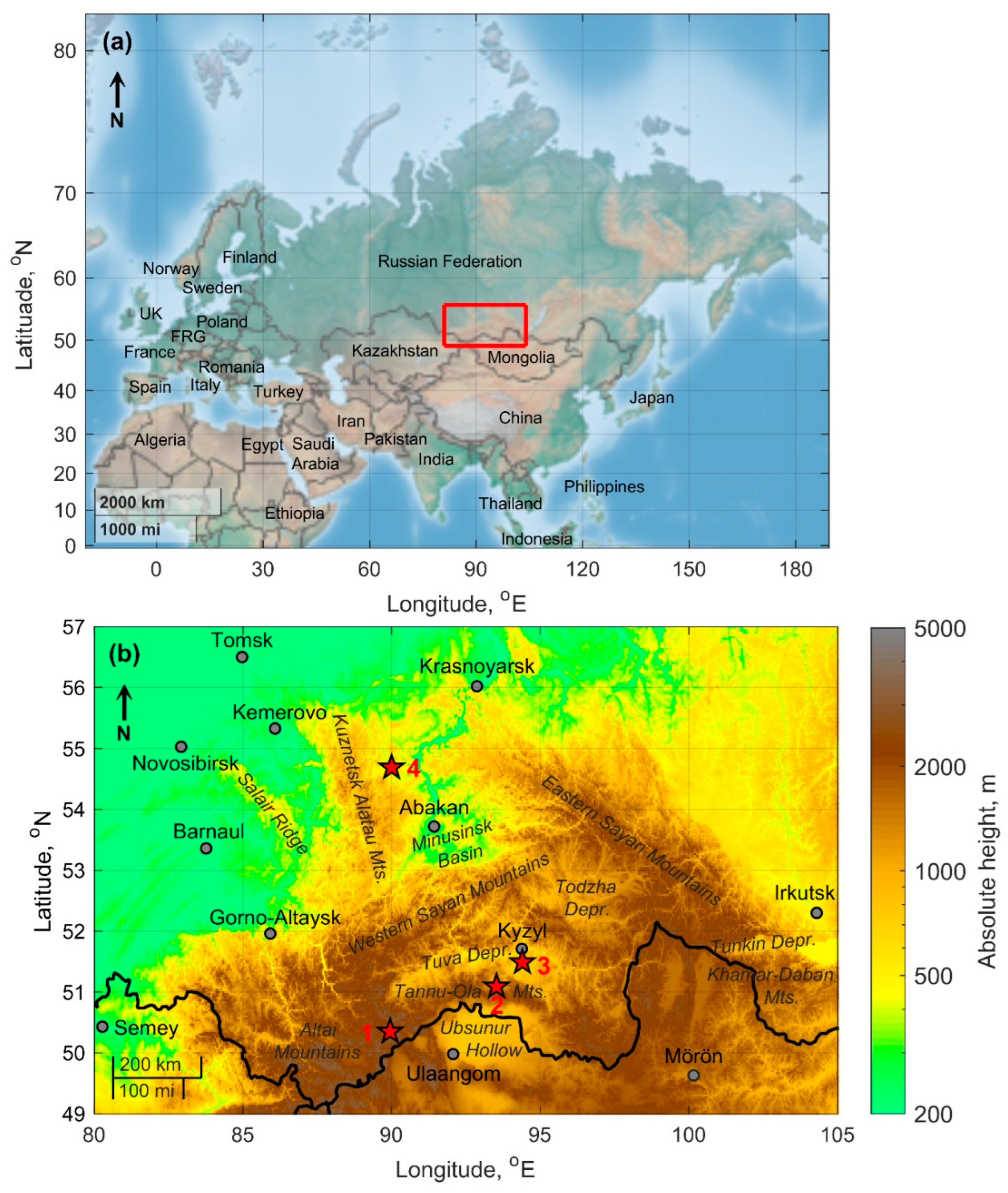
Figure 2.
Box plot (left panels) and histogram (right panels) of the distribution of positive air ion density in fair-weather conditions at observation sites.
Figure 2.
Box plot (left panels) and histogram (right panels) of the distribution of positive air ion density in fair-weather conditions at observation sites.
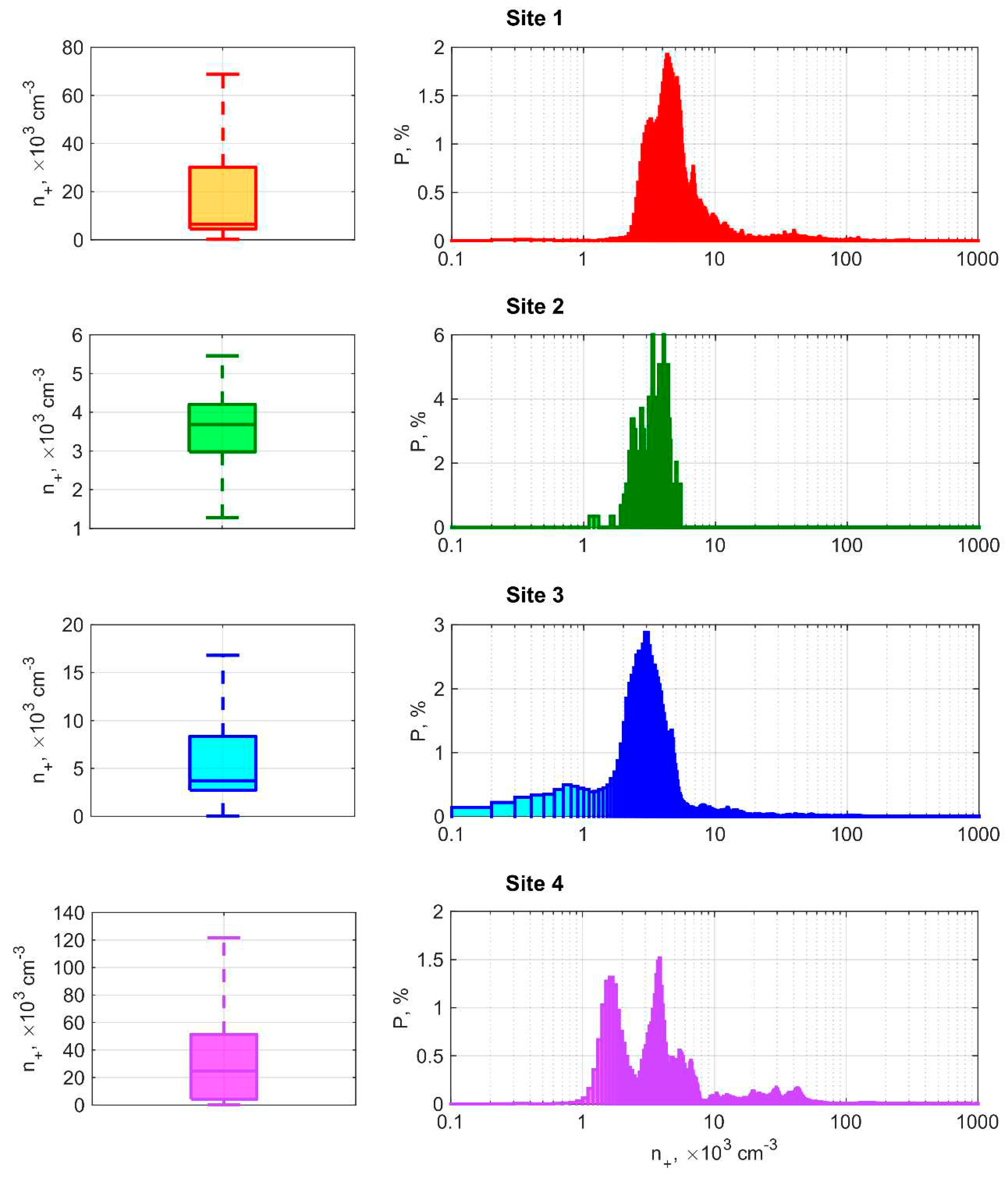
Figure 3.
Diurnal variation of hourly means of positive air ion density in fair-weather conditions at observation sites.
Figure 3.
Diurnal variation of hourly means of positive air ion density in fair-weather conditions at observation sites.
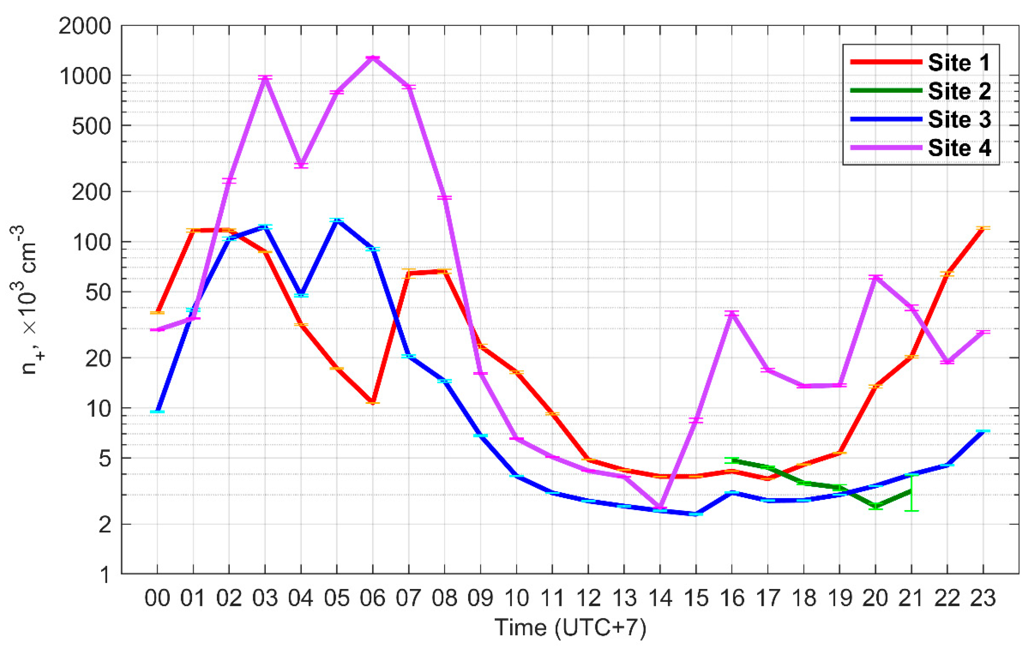
Figure 4.
Box plot (left panels) and histogram (right panels) of the distribution of negative air ion density in fair-weather conditions at observation sites.
Figure 4.
Box plot (left panels) and histogram (right panels) of the distribution of negative air ion density in fair-weather conditions at observation sites.
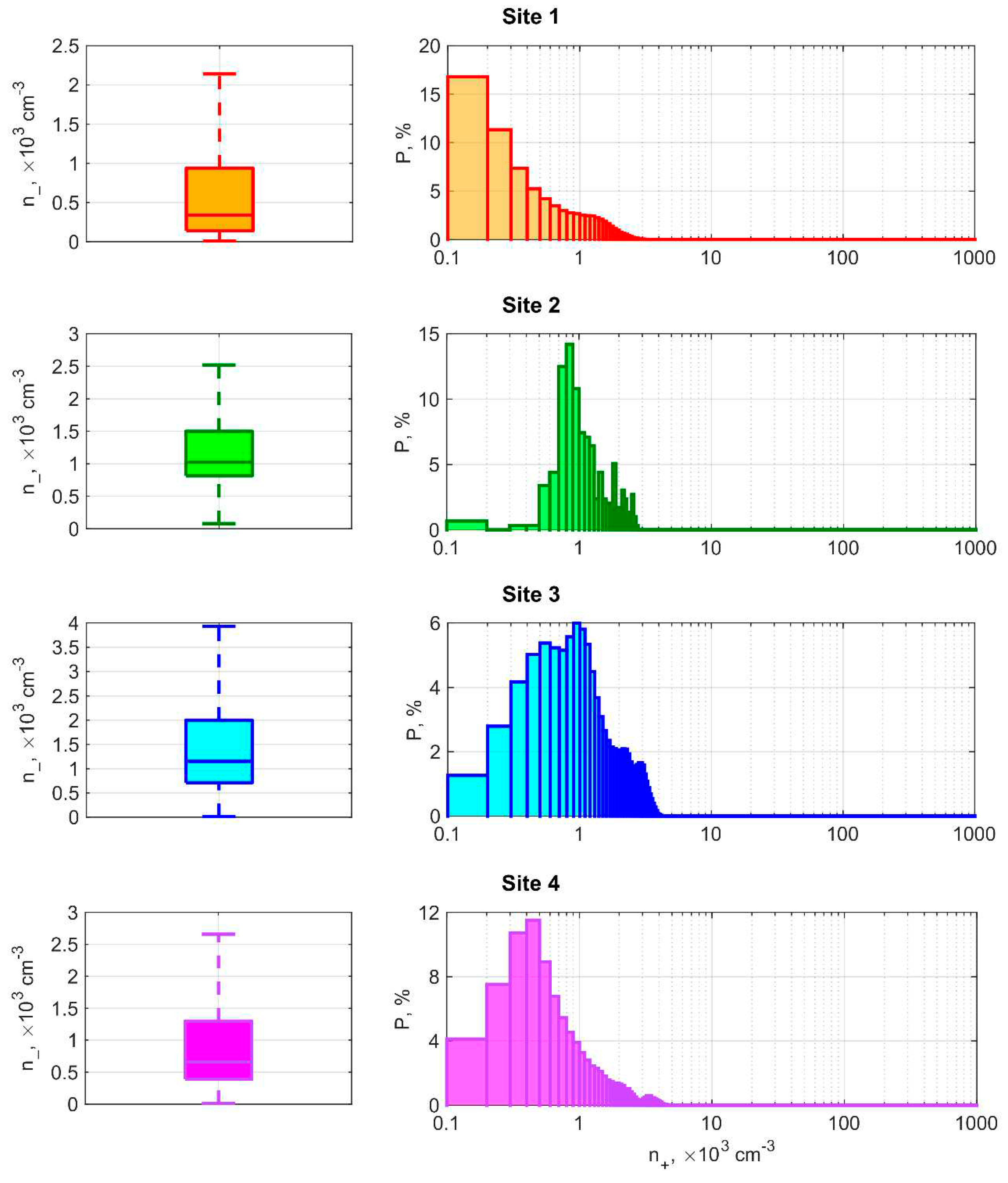
Figure 5.
Diurnal variation of hourly means of negative air ion density in fair-weather conditions at observation sites.
Figure 5.
Diurnal variation of hourly means of negative air ion density in fair-weather conditions at observation sites.
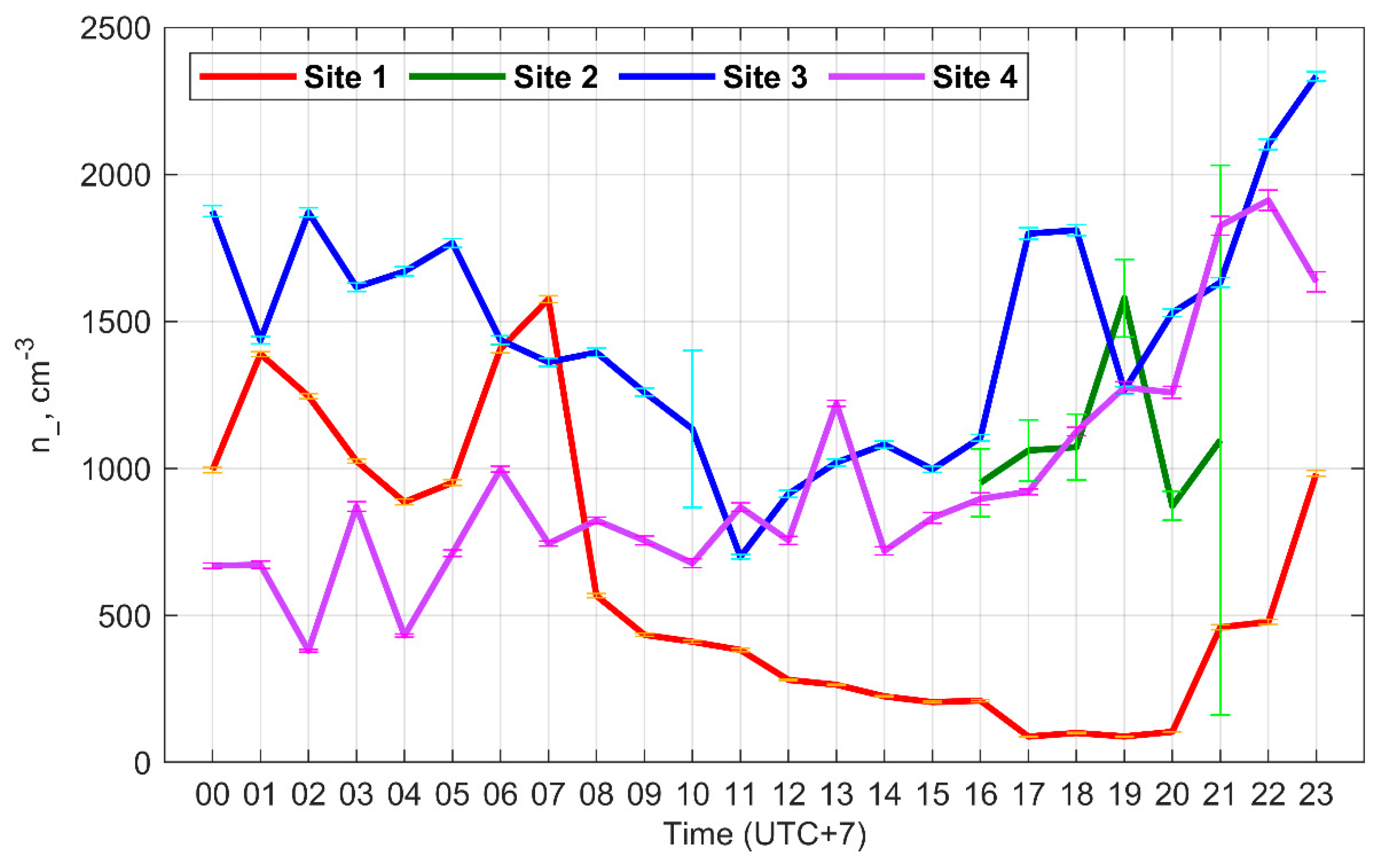
Figure 6.
Box plot (left panels) and histogram (right panels) of the distribution of the potential gradient in fair-weather conditions at observation sites.
Figure 6.
Box plot (left panels) and histogram (right panels) of the distribution of the potential gradient in fair-weather conditions at observation sites.
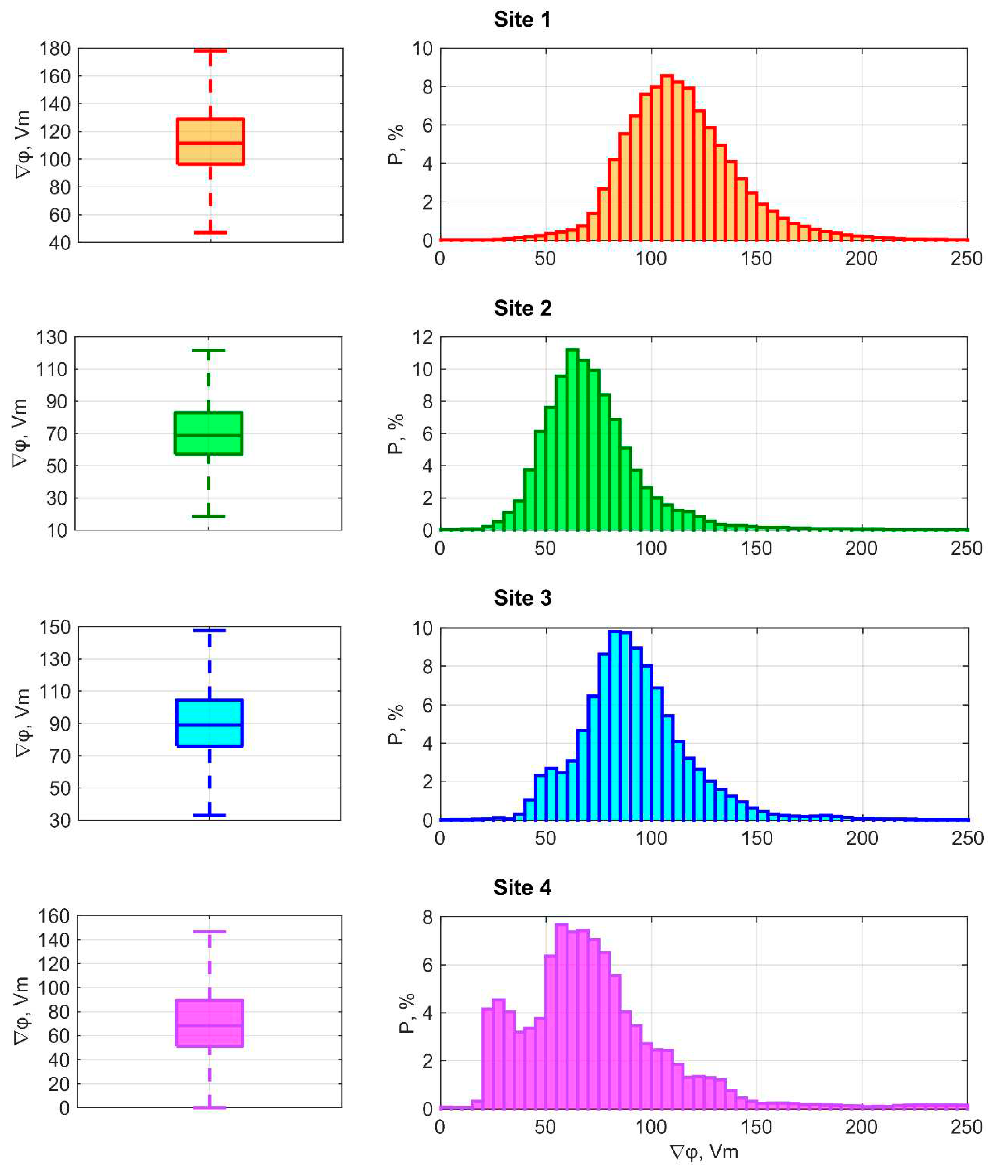
Figure 7.
Diurnal variation of hourly means of potential gradient in fair-weather conditions at observation sites.
Figure 7.
Diurnal variation of hourly means of potential gradient in fair-weather conditions at observation sites.
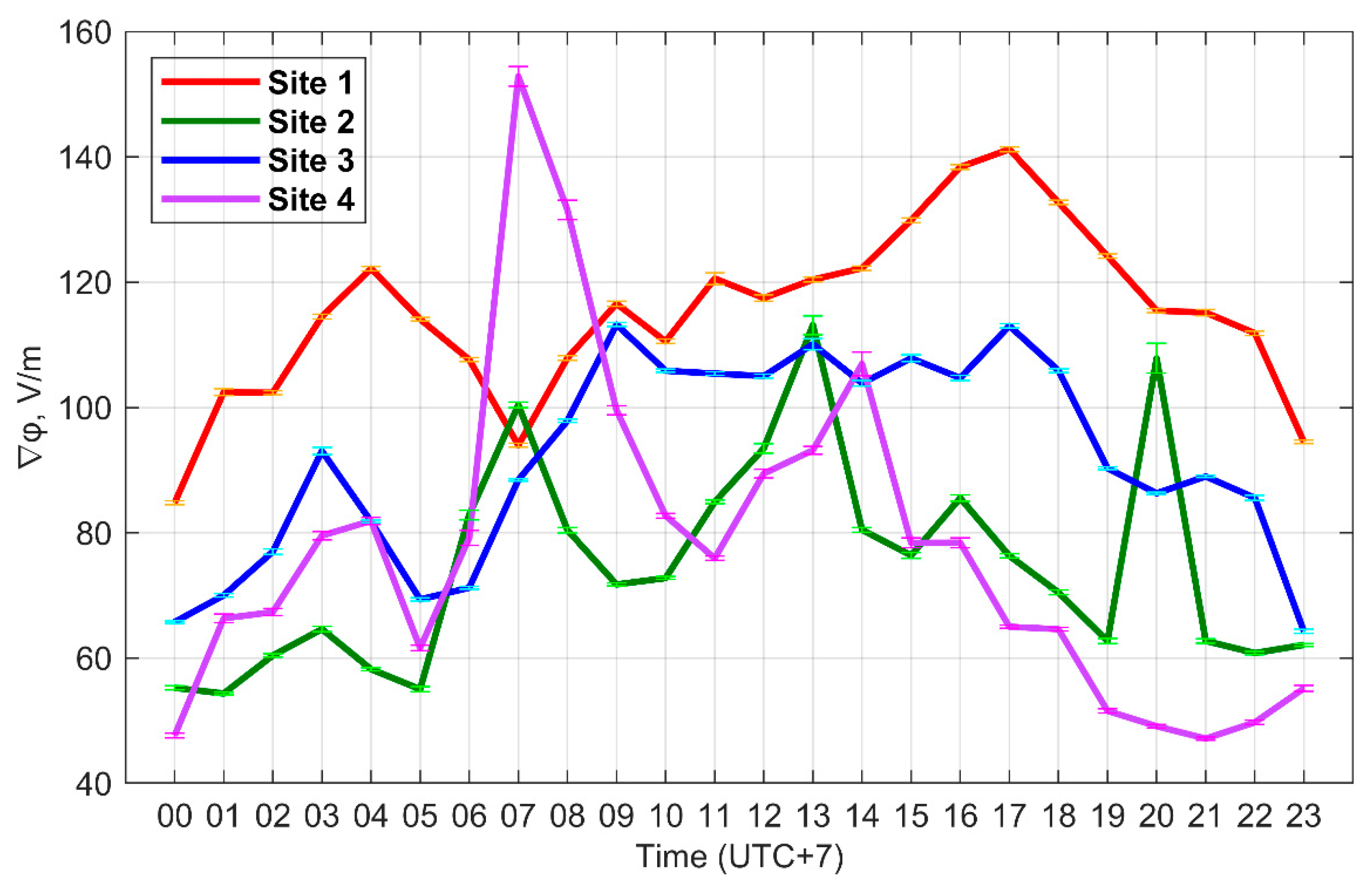
Figure 8.
Diurnal variation of hourly means of conduction current density in fair-weather conditions at observation sites.
Figure 8.
Diurnal variation of hourly means of conduction current density in fair-weather conditions at observation sites.
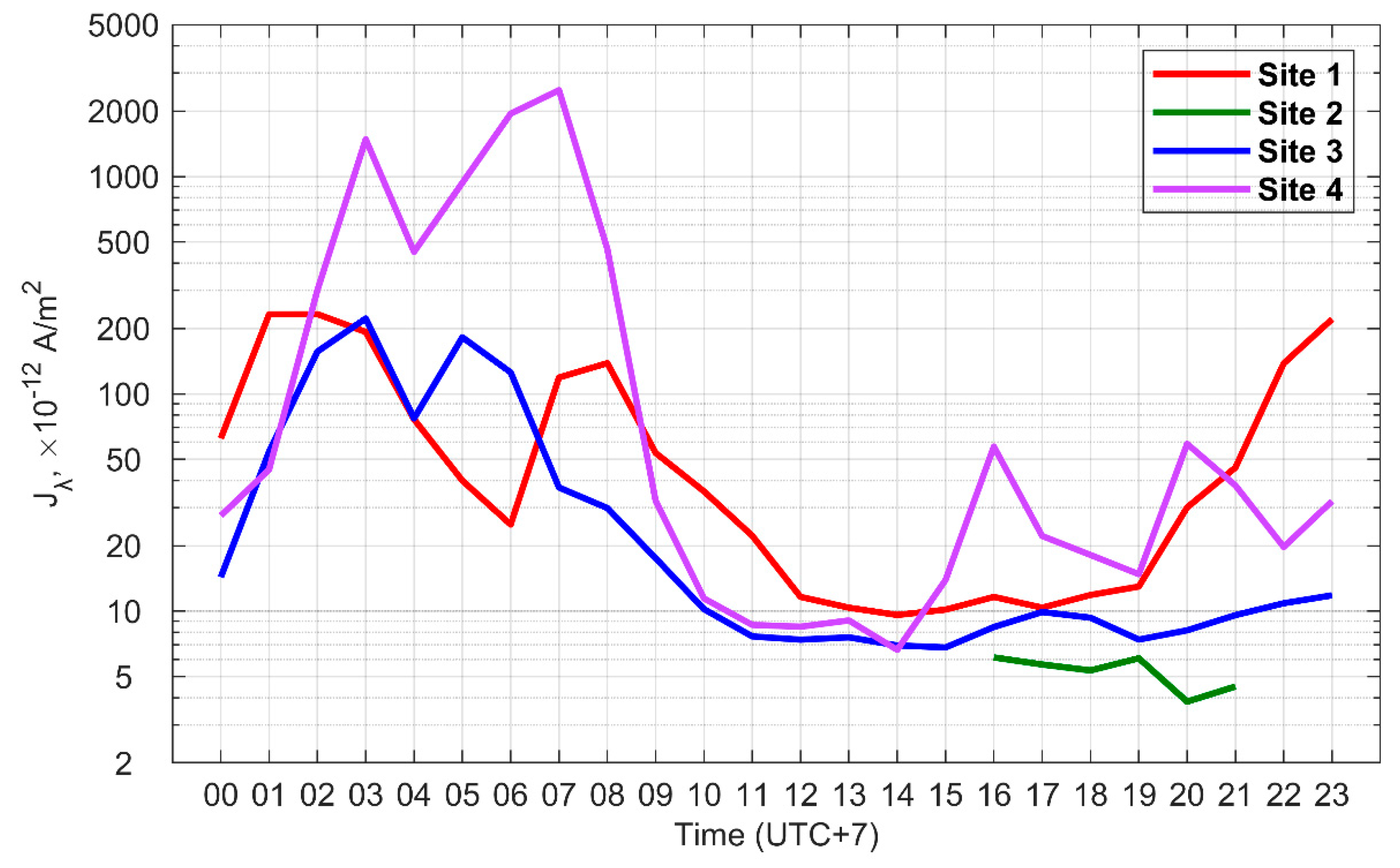
Table 1.
Description of the observation sites.
| Site number | Observation area | Lat., °N | Long., °E | Alt. a.s.l., m | Observation period |
|---|---|---|---|---|---|
| 1 | Plateau near the Mongun-Taiga mountain massif and Khindiktig-Khol lake | 50.4 | 90.0 | 2490 | 24–29.07.2022 |
| 2 | Bayan-Tala tract in the foothills of the Tannu-Ola ridge | 51.1 | 93.5 | 1030 | 19–22.07.2022 |
| 3 | Shol tract in the center of the Tyva depression | 51.5 | 94.4 | 910 | 01–06.08.2022 |
| 4 | Krasnaya Sopka tract between Belyo and Tus salt lakes in the Khakass-Minusinsk basin | 54.7 | 90.0 | 540 | 11–14.08.2022 |
Disclaimer/Publisher’s Note: The statements, opinions and data contained in all publications are solely those of the individual author(s) and contributor(s) and not of MDPI and/or the editor(s). MDPI and/or the editor(s) disclaim responsibility for any injury to people or property resulting from any ideas, methods, instructions or products referred to in the content. |
© 2023 by the authors. Licensee MDPI, Basel, Switzerland. This article is an open access article distributed under the terms and conditions of the Creative Commons Attribution (CC BY) license (http://creativecommons.org/licenses/by/4.0/).
Copyright: This open access article is published under a Creative Commons CC BY 4.0 license, which permit the free download, distribution, and reuse, provided that the author and preprint are cited in any reuse.


