Richard Kerner’s Path Integral Approach Aims to Understand the Self-Organized Matter Agglomeration and Its Translation into the Energy Landscape Kinetics Paradigm

1. Richard Kerner agglomeration model

The method is based in finding the probability of forming certain structural motifs at a certain time from those of the previous step of agglomeration [2]. The method is almost self-explained by giving a simple example. Here we will consider the case of a chalcogen element, say $Se$, doped with a concentration x of another element with well defined coordination, say $As$. Chalcogen atoms belong to the group VI of the periodic table and tend to form large chains, i.e., the coordination of Se atoms is $z_{Se}=2$. The coordination of $As$ is $z_{As}=3$. Experimentally, at the time that RK was working on this compound, it was known that the glass transition temperature ($T_g$), viscosity ($\eta$) and specific heat jump ($\Delta c_p$) were a function of x. Only phenomenological theories were available and it was recognized as an important problem because $T_g$ changes dramatically with small x. In fact, before RK applied his method [28], the explanation of the thousand years old phoenicians recipe for doping sand with certain concentrations of impurities to obtain window glasses remained elusive. It was also clear that network topology played an important role as the bonding energies between impurities and chalcogens were not able to explain the experimental data [18,21,23,31]. At that time, other scientists that arrived to the same conclusion [32,33,34,35]. Eventually, this leads to other advancements like a universal topological law for glass relaxation [36,37] or in the description of liquid glassy melts [38,39] and Boson peak [40,41,42]. These advances eventually proved crucial in describing, designing, and producing over 400 different types of glasses, including those used in tablets, smartphones, and other devices [43].

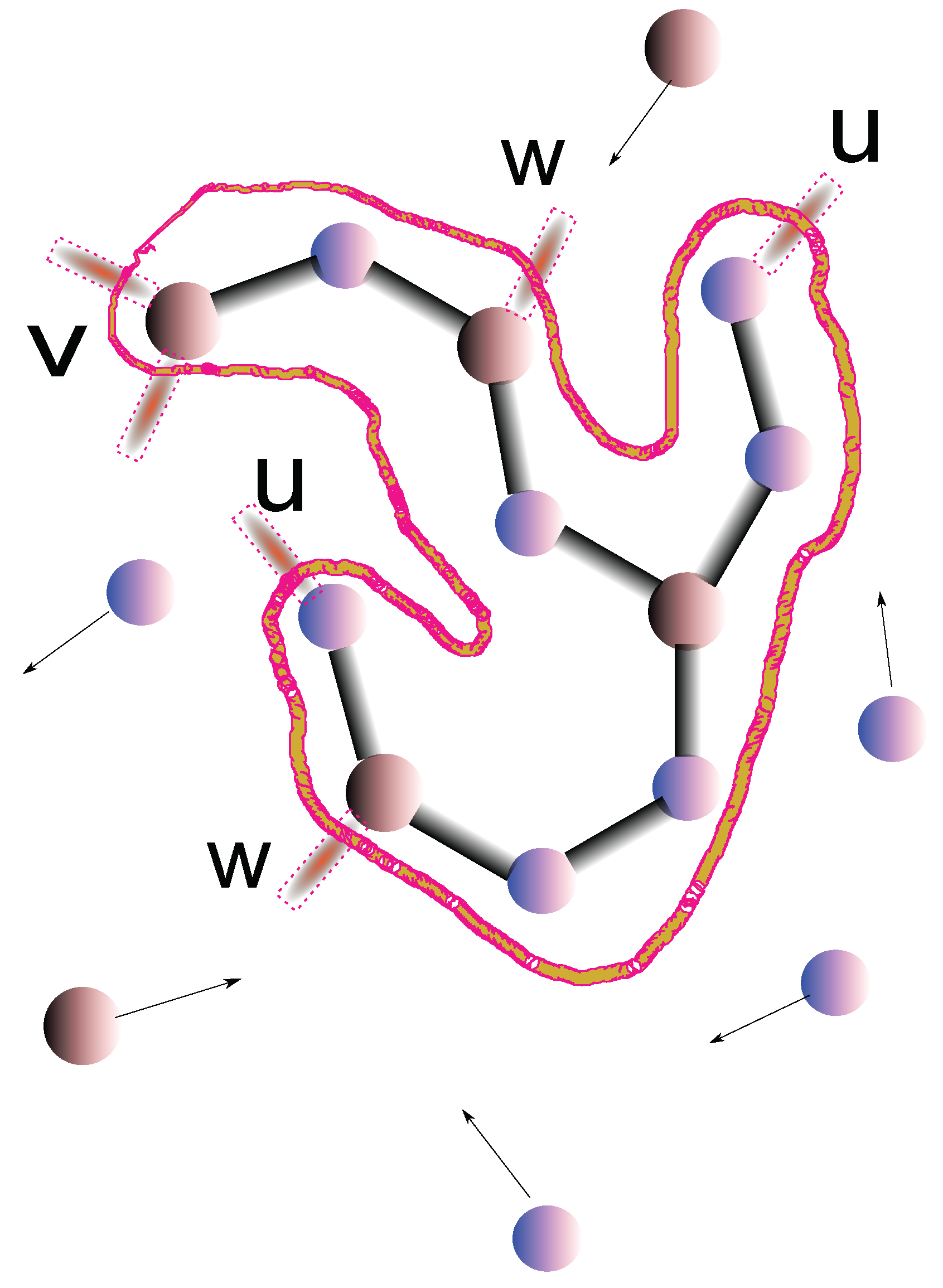
Figure 1. Agglomeration model of ${\mathrm{Se}}_{1-x}$${\mathrm{As}}_x$ glass. A cluster made of Se atoms, with coordination $z_{Se}=2$ and As atoms, with coordination $z_{As}=3$ is indicated by the curve. The unsatisfied bonds at the rim of the cluster are indicated by dotted edges bonds. The three kinds of surface sites u,v,w are indicated. Free atoms in the melt are indicated with arrows that indicate the velocity vector.

Figure 1. Agglomeration model of ${\mathrm{Se}}_{1-x}$${\mathrm{As}}_x$ glass. A cluster made of Se atoms, with coordination $z_{Se}=2$ and As atoms, with coordination $z_{As}=3$ is indicated by the curve. The unsatisfied bonds at the rim of the cluster are indicated by dotted edges bonds. The three kinds of surface sites u,v,w are indicated. Free atoms in the melt are indicated with arrows that indicate the velocity vector.

Assuming that the system is melted at high temperatures, to form a glass the system is cooled down with a certain protocol, i.e., the temeprature T is a function of time t. Usually, $T\left(t\right)=T_0-Rt$ where $T_0$ is the initially temperature and R the cooling rate. At a certain time, the atoms will begin to interact with a nucleation center and form bonds. Each bond has a definite energy, $ϵ$ for Se-Se bonds, $\eta$ for Se-As bonds and $\alpha$ for As-As bonds. However, the probability of forming bonds, according to RK depends on,

• The number of ways in which a bond can be made.
• The Bond Energy;
• The concentration of atomic species
• The temperature

These are clearly very common sense physical inputs. Now consider a nucleation center. It will contain unsaturated Se bonds with one free bond, call them sites of type u, and As atoms with two and one available free bonds, called v and w sites respectively. The different possible terminations of the rim can be considered as possible states of a vector $\left|p\right(t)\rangle$ which encodes the probability of states on the rim. The probabilities after a new step of agglomeration are then obtained as in a Markov process, i..e, by applying a transition matrix to the rim state vector that contains the probability of making a new bond, i.e., we have,

$$\left|p\right(t+dt)\rangle =\mathbf{M}(t\left)\right|p\left(t\right)\rangle$$

(1)

where,

$$|p\left(t\right)\rangle ={(p_u,p_v,p_w)}^T$$

(2)

and $\mathbf{M}\left(t\right)$ is an stochastic matrix as each column must be normalized to one in order to ensure probability normalization at each step. The elements of $\mathbf{M}\left(t\right)$ are called the transition probabilities and as we will discuss later on, are the source of the debate. I will leave its discussion to a separate section. RK proposed that such transition probabilities of attaching Se or As into sites of type u,v or w on the cluster surface were given by taking into account in its simplest way all the four entries of the physical input list, i.e., the elements of $\mathbf{M}\left(t\right)$ are,

• u+Se; $M_{11}\left(t\right)=\frac{z_{Se}(1-x)e^{-ϵ/T}}{Q_1\left(t\right)}$
• u+As; $M_{21}\left(t\right)=\frac{z_{As}x{e}^{-\eta /T}}{Q_1\left(t\right)}$
• v+Se; $M_{31}\left(t\right)=\frac{z_{Se}(1-x)e^{-ϵ/T}}{Q_2\left(t\right)}$
• v+As; $M_{22}\left(t\right)=\frac{2z_{As}x{e}^{-ϵ/T}}{Q_2\left(t\right)}$
• w+Se; $M_{31}\left(t\right)=\frac{z_{Se}(1-x)e^{-ϵ/T}}{Q_3\left(t\right)}$
• w+As; $M_{32}\left(t\right)=\frac{z_{As}x{e}^{-ϵ/T}}{Q_3\left(t\right)}$.

and all others elements are zero. Here $Q_1\left(T\right),Q_2\left(T\right),Q_3\left(T\right)$ are the normalization factors that ensure column normalization of $\mathbf{M}\left(t\right)$. Note that here we used the most powerful version of the method [24,27] that was made after RK made several works in which the calculations were made for several systems by hand, i.e., by performing the agglomeration steps, computing probabilities and sometime discarding some low probability configurations [20,22]. At a certain point, a self-consistent equation was found that defined the temperature at which the cluster was able to grow.

In terms of Markov chains, the solution is easy. As $\mathbf{M}\left(t\right)$ is stochastic, it has an eigenvector with eigenvalue one which will dominate others after successive applications of $\mathbf{M}\left(t\right)$ onto any given state vector [44]. Therefore, we compute the eigenvector with eigenvalue one and from it, obtain the stationary state of the rim. The glass transition temperature can be found for example by looking for a jump in the specific heat [27]. The method is well documented in many papers. It was able to find the concentration of boroxol rings, viscosity, specific heat [27] of ${\mathrm{B}}_2$${\mathrm{O}}_3$ glass and even the modified empirically observed Gibbs-DiMarzio equation for chalcogenide glasses [24]. In the following section, we will discuss some controversial issues and their relationship in terms of the energy landscape kinetics picture and path integrals.

2. Translation to the energy landscape paradigm and path integrals

Some objections have been raised against the RK and the stochastic matrix method. The main criticism are,

• The method is too simple to work.
• Topology is taken into account in a very simplistic way, just by counting the number of bonding possibilities.
• The transition elements of the stochastic matrix use Boltzmann factors, but agglomeration is usually a non-equilibrium processes.

Point 1 of the previous list is not a problem per se and in fact, according to the Occam’s razor, is a benefit. Point 2 has huge experimental support, as for example, the boiling temperature of isomers depend upon such number [45]. Point 3 is the most difficult to answer, but to be fair, it turns out to be controversial also for the energy landscape paradigm.

Let us now build the connection between the RK method and the energy landscape. Consider that any thermodynamical system evolves in the energy landscape exactly as given by eq. (1). The differences are in the details. $\left|p\right(t)\rangle$ represents a probability vector in which each component gives the probability of the system to be in a state, say j, with energy $E_j$ and mechanical coordinates $\{q_1,q_2,...,q_{3N},{\Pi }_1,{\Pi }_2,...,{\Pi }_{3N}\}$. $q_l$ are the generalized space coordinates and ${\Pi }_l$ the generalized momenta of N atoms [5,9,14,15]. The interaction is given by a potential $V(q_1,q_2,...,q_{3N})$. When compared with the entries of the RK method, the situation looks hopeless. However in most physical cases the states are grouped in basins which evolve around inherent, dominant configurations. As an example, we already cited the case of proteins which although very complex are described by two level systems [10]. In molecular simulations, the phase space is partitioned in parcels and the size of $\left|p\right(t)\rangle$ is dramatically reduced to a bunch of configurations as in the RK method [46].

Now the connection between RK method, the energy landscape and a path integral approach is much clear. By writing eq. (1) as,

$$\frac{d}{dt}|p\left(t\right)\rangle =\mathbf{W}\left(t\right)|p\left(t\right)\rangle$$

(3)

where $\mathbf{M}\left(t\right)\equiv \mathbf{W}\left(t\right)dt+1$ and $dt$ is the time interval, the evolution after time t can be obtained from a recursive application of $\mathbf{W}\left(t\right)$ and the formal solution of eq. (3) is,

$$|p\left(t\right)\rangle =\mathcal{T}{e}^{{\int }_{t_0}^t\mathbf{W}\left(t\right)dt}|p\left(t_0\right)\rangle$$

(4)

Notice that a "time order operator" $\mathcal{T}$ was introduced. It takes into account the non-conmmutative nature of the operator $\mathbf{W}\left(t\right)$ at different times. This path integral is akin to the time evolution of a quantum mechanical system [47]. If the linear cooling protocol $T\left(t\right)$ is used where $T\left(t_0\right)=T_0$, we can define the path integral in temperature,

$$|p\left(T\right)\rangle =\mathcal{T}{e}^{-\frac{1}{R}{\int }_{T_0}^T\mathbf{W}\left(T\right)dT}|p\left(T_0\right)\rangle$$

(5)

Notice that here R plays the role of the Planck constant ℏ when compared with the quantum case. Thus we see that the RK method relies on a clever way of identifying the states that play a prominent role. Agglomeration centers represent states in which a certain subset of generalized coordinates, denoted as $q_1,q_2,\dots ,q_{3N}$, are held fixed or frozen. This intuitive idea has been confirmed by using an automated approach, based on self-organizing neural nets [48]. The result: "the conformational information from 30,000 samples from the full trajectories was retained in relatively few resultant clusters" [48].

3. Transition probabilities of the agglomeration process

As we observed in the previous section, there are no major issues or problems with the RK method when compared to the energy landscape model. The primary distinction lies in the manual identification of relevant states, a process that is often facilitated by the computational power available in more complex studies [9,14,15]. As mentioned earlier, the main concern revolves around computing the elements of the matrix $\mathbf{M}\left(t\right)$, which has been addressed here in the context of $Se-As$ glasses. However, it’s important to note that this is not a unique problem specific to the RK method. Markov state modeling has often been considered more of an art than a science [49].

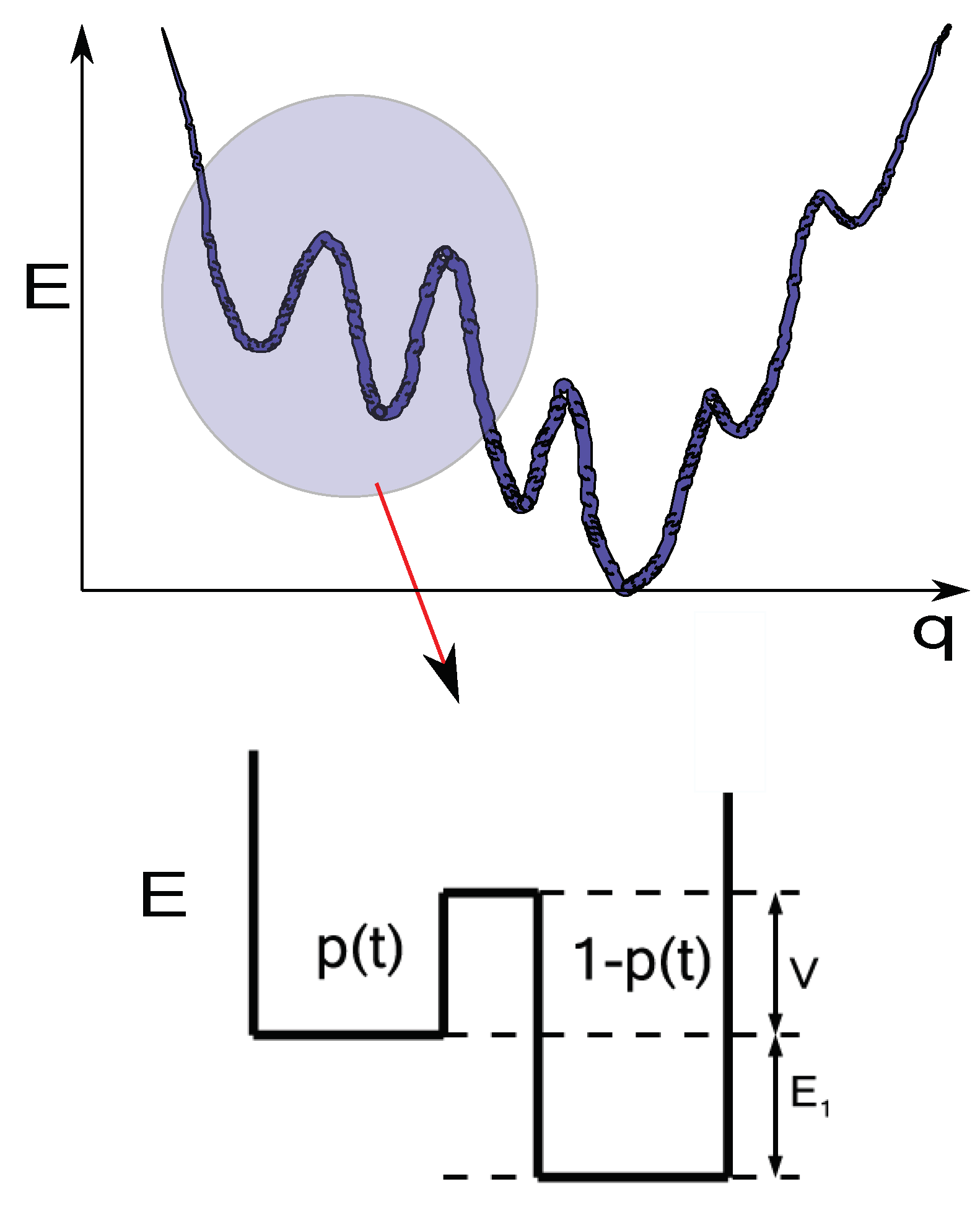
To understand the Boltzmann factors of the RK method, we consider that locally in a certain energy range, the energy landscape can be seen as a typical two level energy landscape model [46,50,51]. Figure 2 presents a sketch of such idea. The system is not at equilibrium but is in thermal contact with a bath at a temperature $T\left(t\right)$ that varies with time. The energy landscape kinetic equation Eq. (3) can be locally written as,

$$\frac{d}{dt}\left(\begin{array}{c}-p\left(t\right)\\ p\left(t\right)\end{array}\right)=\left(\begin{array}{cc}-{\Gamma }_{\uparrow \downarrow }\left(t\right)& {\Gamma }_{\downarrow \uparrow }\left(t\right)\\ {\Gamma }_{\uparrow \downarrow }\left(t\right)& -{\Gamma }_{\downarrow \uparrow }\left(t\right)\end{array}\right)\left(\begin{array}{c}1-p\left(t\right)\\ p\left(t\right)\end{array}\right)$$

(6)

where $1-p\left(t\right)$ is the low energy, set to $E_0=0$ for conviencience, state probability occupation, and $p\left(t\right)$ is the same quantity but for the high energy state with energy $E_1$ ( see Figure 2). These states are separated by a potential barrier of height V.

The element ${\Gamma }_{\uparrow \downarrow }\left(t\right)$ is the transition rate from the lower to high energy state, and the inverse process has rate ${\Gamma }_{\downarrow \uparrow }\left(t\right)$. According to non-equilibrium thermodynamics and neglecting quantum tunelling [50,52], ${\Gamma }_{\uparrow \downarrow }\left(t\right)=e^{-\frac{E_1}{T\left(t\right)}}{\Gamma }_{\downarrow \uparrow }$ and ${\Gamma }_{\downarrow \uparrow }\left(t\right)={\Gamma }_0{e}^{-\frac{V}{T\left(t\right)}}$. ${\Gamma }_0$ is the oscillation frequency on each energy well and gives a natural time-scale for the problem ${\tau }_0\equiv {\Gamma }_0^{-1}$. Now we see that the Boltzmann factor appear not due to thermal equilibrium, instead, is a property derived from the contact with a bath which has a well defined temperature [52]. The price paid is the factor that contains V, which is the potential barrier separating both states. To see this, we show how for the system in equilibrium, V disappears from the picture.

Assuming thermal equilibrium means here a quasistatic cooling, obtained by setting $d\left|p\right(t)\rangle /dt\approx 0$. As the temperature can be considered fixed, from the eigenvector with eigenvalue one of $\mathbf{M}\left(t\right)$ we obtain the equilibrium population $p^e\left(T\right)=p^e\left(T\left(t\right)\right)$,

$$p^e\left(T\right)=\frac{{\Gamma }_{\uparrow \downarrow }\left(T\left(t\right)\right)}{({\Gamma }_{\uparrow \downarrow }\left(T\left(t\right)\right)+{\Gamma }_{\downarrow \uparrow })\left(T\left(t\right)\right)}=\frac{e^{-\frac{E_1}{T}}}{1+e^{-\frac{E_1}{T}}},$$

(7)

which reproduces the result obtained from an equilibrium partition function, without any final reference to V. Let us now discuss the non-equilibrium cooling. Eq. (6) reduces to one equation,

$$\frac{dp\left(t\right)}{dt}=f(t,p)$$

(8)

where,

$$f(t,p)={\Gamma }_0{e}^{-\frac{V}{T\left(t\right)}}[(1-p\left(t\right))e^{-\frac{E}{T\left(t\right)}}-1].$$

(9)

The equilibrium population $p^e\left(T\right)$ is recovered from the roots of $f(p,T)$. For a fixed time, the nature of the stability around the equilibrium solution is given by the sign of the derivative with respect to p evaluated at equilibrium,

$${\left.\frac{\partial f(t,p)}{\partial p}\right|}_{p=p^e\left(t\right)}=-{\Gamma }_0{e}^{-\frac{(V+E_1)}{T\left(t\right)}}<0$$

(10)

showing that indeed the solutions are stable and converge to $p^e\left(T\right)$. By looking at $f(t,p)$, we see that the term in square brackets is the equilibrium condition while the term ${\Gamma }_0{e}^{-\frac{V}{T\left(t\right)}}$ plays the role of an inverse relaxation time $\tau$. For $V<<T\left(t\right)=T_0-Rt$, the relaxation time is constant $\tau \approx {\tau }_0={\Gamma }_0^{-1}$ and we can use the local equilibrium Boltzmann factors. In a funnel landscape along the coordinate reaction direction, the barriers V are expected to be $V<<T$ during the agglomeration process. This is specially true for chalcogenide glasses, as the topology in real space is related with the energy barriers via constraint, rigidity theory [39,53,54,55,56]. So the lack of atomic constraints means that there is a thermodynamic finite amount of $V\approx 0$ channels in configurational space where the present approach can be used [39,57]. Therefore, the use of Boltzmann factors by the RK theory appears to be well justified, explaining the striking agreement when compared with experimental data. Once the solid is formed, the approximation breaks down as the relaxation time can no longer be supposed constant. This can be seen by writing Eq. (6) as,

$$\delta \frac{dp\left(x\right)}{dx}=\frac{1}{{(lnx)}^2}[-x^{\mu }+(1+x^{\mu })p\left(x\right)]$$

(11)

using the definitions,

$$x=exp(-V/T),\mu =E_1/V$$

(12)

where $\delta =RV/{\Gamma }_0{T}_0$ is an adimensional cooling rate. For $\delta =0$ it is easy to see that the equilibrium case is recovered. A power series expansion in powers $\delta$ reveals a divergence in the first order in a region of size determined by $x_b=\delta {(ln{x}_b)}^2$ associated with temperatures in which the system is frozen in the upper state, indicating a glassy, solid, behavior. The evolution can also be written in terms of the path integral,

$$|p\left(x\right)\rangle =\mathcal{T}{e}^{-\frac{1}{\delta }{\int }_{x_0}^x\mathbf{W}\left(x\right)dx}|p\left(x_0\right)\rangle$$

(13)

with initial condition $x_0=exp(-V/T_0)$ and $\mathbf{W}\left(x\right)$ given by,

$$\mathbf{W}\left(x\right)=\frac{1}{{(lnx)}^2}\left(\begin{array}{cc}-x^{1+\mu }& x\\ x^{1+\mu }& -x\end{array}\right).$$

(14)

For $x>>x_b$, $x\approx 1$ and $\mathbf{W}\left(x\right)$ becomes a constant matrix. What we observe here is that the departure from the equilibrium case results in a renormalization of the weights, due to the presence of a barrier V, with respect to the Boltzmann factor.

4. Conclusions

In this work I made a short review of the Richard Kerner’s path integral approach aims to understand the self-organized matter agglomeration. It was shown how it can be translated into the energy landscape kinetics paradigm as the RK method identifies most probable clusters and the state of its surface. Then a revision was made concerning the transition matrix elements of the associated stochastic matrix. As it was discussed, the most controversial issue is the use of Boltzmann factors. However, such issue disappears if the transition barriers along the reaction coordinate of the energy landscape are not very high when compared with the thermal energy as happens in funnel-like energy landscapes.

References

- Chaikin, P.; Lubensky, T. Principles of Condensed Matter Physics; Cambridge University Press, 2000.
- Kerner, R. Models of Agglomeration and Glass Transition; Imperial College Press, 2006.
- Jooss, C. Self-organization of Matter: A dialectical approach to evolution of matter in the microcosm and macrocosmos; De Gruyter STEM, De Gruyter, 2020. https://www.pnas.org/doi/pdf/10.1073/pnas.0608517103.
- Sethna, J. Statistical Mechanics: Entropy, Order Parameters and Complexity; Oxford Master Series in Physics, OUP Oxford, 2006.
- Rylance, G.J.; Johnston, R.L.; Matsunaga, Y.; Li, C.B.; Baba, A.; Komatsuzaki, T. Topographical complexity of multidimensional energy landscapes. Proceedings of the National Academy of Sciences 2006, 103, 18551–18555. [Google Scholar] [CrossRef] [PubMed]
- Parisi, G.; Urbani, P.; Zamponi, F. Theory of Simple Glasses: Exact Solutions in Infinite Dimensions; Cambridge University Press, 2020.
- Welch, R.S.; Zanotto, E.D.; Wilkinson, C.J.; Cassar, D.R.; Montazerian, M.; Mauro, J.C. Cracking the Kauzmann paradox. Acta Materialia 2023, 254, 118994. [Google Scholar] [CrossRef]
- Bore, S.L.; Paesani, F. Realistic phase diagram of water from first principles data-driven quantum simulations. Nature Communications 2023, 14, 3349. [Google Scholar] [CrossRef] [PubMed]
- Roder, K.; Joseph, J.A.; Husic, B.E.; Wales, D.J. Energy Landscapes for Proteins: From Single Funnels to Multifunctional Systems. Advanced Theory and Simulations 2019, 2, 1800175. https://onlinelibrary.wiley.com/doi/pdf/10.1002/adts.201800175. [CrossRef]
- Tapia-Rojo, R.; Mora, M.; Board, S.; Walker, J.; Boujemaa-Paterski, R.; Medalia, O.; Garcia-Manyes, S. Enhanced statistical sampling reveals microscopic complexity in the talin mechanosensor folding energy landscape. Nature Physics 2023, 19, 52–60. [Google Scholar] [CrossRef] [PubMed]
- Dobson, C.M. Protein-misfolding diseases: Getting out of shape. Nature 2002, 418, 729–730. [Google Scholar] [CrossRef] [PubMed]
- Levinthal, C. Are there pathways for protein folding? J. Chim. Phys. 1968, 65, 44–45. [Google Scholar] [CrossRef]
- Dill, K.A.; Chan, H.S. From Levinthal to pathways to funnels. Nature Structural Biology 1997, 4, 10–19. [Google Scholar] [CrossRef] [PubMed]
- Wales, D.J. Discrete path sampling. Molecular Physics 2002, 100, 3285–3305. [Google Scholar] [CrossRef]
- Roder, K.; Wales, D.J. The Energy Landscape Perspective: Encoding Structure and Function for Biomolecules. Frontiers in Molecular Biosciences 2022, 9. [Google Scholar] [CrossRef]
- Hiranuma, N.; Park, H.; Baek, M.; Anishchenko, I.; Dauparas, J.; Baker, D. Improved protein structure refinement guided by deep learning based accuracy estimation. Nature Communications 2021, 12, 1340. [Google Scholar] [CrossRef] [PubMed]
- Susskind, L. The Cosmic Landscape: String Theory and the Illusion of Intelligent Design; Little, Brown, 2008.
- Kerner, R. Phenomenological Lagrangian for the amorphous solid state. Phys. Rev. B 1983, 28, 5756–5761. [Google Scholar] [CrossRef]
- Kerner, R.; dos Santos, D.M.L.F. Nucleation and amorphous and crystalline growth: A dynamical model in two dimensions. Phys. Rev. B 1988, 37, 3881–3893. [Google Scholar] [CrossRef] [PubMed]
- Kerner, R.; Penson, K.A.; Bennemann, K.H. Model for the Growth of Fullerenes (C60, C70) from Carbon Vapour. Europhysics Letters 1992, 19, 363. [Google Scholar] [CrossRef]
- Kerner, R.; Micoulaut, M. On the glass transition temperature in covalent glasses. Journal of Non-Crystalline Solids 1997, 210, 298–305. [Google Scholar] [CrossRef]
- Kerner, R. Nucleation and growth of fullerenes. Computational Materials Science 1994, 2, 500–508, Theory of Atomic and Molecular Clusters. [Google Scholar] [CrossRef]
- Kerner, R. Geometrical approach to the glass transition problem. Journal of Non-Crystalline Solids 1985, 71, 19–27, Effects of Modes of Formation on the Structure of Glass. [Google Scholar] [CrossRef]
- Naumis, G.G.; Kerner, R. Stochastic matrix description of glass transition in ternary chalcogenide systems. Journal of Non-Crystalline Solids 1998, 231, 111–119. [Google Scholar] [CrossRef]
- Kerner, R.; Naumis, G.G. Stochastic matrix description of the glass transition. Journal of Physics: Condensed Matter 2000, 12, 1641. [Google Scholar] [CrossRef]
- dos Santos-Loff, D.M.; Micoulaut, M.; Kerner, R. Statistics of Boroxol Rings in Vitreous Boron Oxide. Europhysics Letters 1994, 28, 573. [Google Scholar] [CrossRef]
- Barrio, R.A.; Kerner, R.; Micoulaut, M.; Naumis, G.G. Evaluation of the concentration of boroxol rings in vitreous by the stochastic matrix method. Journal of Physics: Condensed Matter 1997, 9, 9219. [Google Scholar] [CrossRef]
- Phillips, J.C.; Kerner, R. Structure and function of window glass and Pyrex. The Journal of Chemical Physics 2008, 128, 174506. https://pubs.aip.org/aip/jcp/article-pdf/doi/10.1063/1.2805043/14841170/174506_1_online.pdf. [CrossRef] [PubMed]
- Kerner, R. Self-Assembly of Icosahedral Viral Capsids: the Combinatorial Analysis Approach. Mathematical Modelling of Natural Phenomena 2011, 6, 136–158. [Google Scholar] [CrossRef]
- Aldrovandi, R. Special Matrices of Mathematical Physics: Stochastic, Circulant, and Bell Matrices; World Scientific, 2001.
- Micoulaut, M.; Naumis, G.G. Glass transition temperature variation, cross-linking and structure in network glasses: A stochastic approach. Europhysics Letters (EPL) 1999, 47, 568–574. [Google Scholar] [CrossRef]
- Phillips, J. Topology of covalent non-crystalline solids I: Short-range order in chalcogenide alloys. Journal of Non-Crystalline Solids 1979, 34, 153–181. [Google Scholar] [CrossRef]
- Thorpe, M. Continuous deformations in random networks. Journal of Non-Crystalline Solids 1983, 57, 355–370. [Google Scholar] [CrossRef]
- He, H.; Thorpe, M.F. Elastic Properties of Glasses. Phys. Rev. Lett. 1985, 54, 2107–2110. [Google Scholar] [CrossRef] [PubMed]
- Boolchand, P.; Bauchy, M.; Micoulaut, M.; Yildirim, C. Topological Phases of Chalcogenide Glasses Encoded in the Melt Dynamics (Phys. Status Solidi B 6/2018). physica status solidi (b) 2018, 255, 1870122. [Google Scholar] [CrossRef]
- Naumis, G.G.; Cocho, G. The tails of rank-size distributions due to multiplicative processes: from power laws to stretched exponentials and beta-like functions. New Journal of Physics 2007, 9, 286. [Google Scholar] [CrossRef]
- Naumis, G.; Phillips, J. Bifurcation of stretched exponential relaxation in microscopically homogeneous glasses. Journal of Non-Crystalline Solids 2012, 358, 893–897. [Google Scholar] [CrossRef]
- Huerta, A.; Naumis, G.G. Evidence of a glass transition induced by rigidity self-organization in a network-forming fluid. Phys. Rev. B 2002, 66, 184204. [Google Scholar] [CrossRef]
- Naumis, G.G. Energy landscape and rigidity. Phys. Rev. E 2005, 71, 026114. [Google Scholar] [CrossRef] [PubMed]
- Flores-Ruiz, H.M.; Naumis, G.G. The transverse nature of the Boson peak: A rigidity theory approach. Physica B: Condensed Matter 2013, 418, 26–31. [Google Scholar] [CrossRef]
- Flores-Ruiz, H.M.; Naumis, G.G.; Phillips, J.C. Heating through the glass transition: A rigidity approach to the boson peak. Phys. Rev. B 2010, 82, 214201. [Google Scholar] [CrossRef]
- Flores-Ruiz, H.M.; Naumis, G.G. Excess of low frequency vibrational modes and glass transition: A molecular dynamics study for soft spheres at constant pressure. The Journal of Chemical Physics 2009, 131, 154501. [Google Scholar] [CrossRef] [PubMed]
- Mauro, J.C.; Yue, Y.; Ellison, A.J.; Gupta, P.K.; Allan, D.C. Viscosity of glass-forming liquids. Proceedings of the National Academy of Sciences 2009, 106, 19780–19784. https://www.pnas.org/content/106/47/19780.full.pdf. [CrossRef] [PubMed]
- Van Kampen, N. Stochastic Processes in Physics and Chemistry; North-Holland Personal Library, Elsevier Science, 1992.
- Pauling, L. General Chemistry; Dover Books on Chemistry, Dover Publications, 2014.
- Huse, D.A.; Fisher, D.S. Residual Energies after Slow Cooling of Disordered Systems. Phys. Rev. Lett. 1986, 57, 2203–2206. [Google Scholar] [CrossRef]
- Weber, M.F.; Frey, E. Master equations and the theory of stochastic path integrals. Reports on Progress in Physics 2017, 80, 046601. [Google Scholar] [CrossRef]
- Karpen, M.E.; Tobias, D.J.; Brooks, C.L.I. Statistical clustering techniques for the analysis of long molecular dynamics trajectories: analysis of 2.2-ns trajectories of YPGDV. Biochemistry 1993, 32, 412–420. [Google Scholar] [CrossRef] [PubMed]
- Husic, B.E.; Pande, V.S. Markov State Models: From an Art to a Science. Journal of the American Chemical Society 2018, 140, 2386–2396. [Google Scholar] [CrossRef] [PubMed]
- Langer, S.A.; Sethna, J.P. Entropy of Glasses. Phys. Rev. Lett. 1988, 61, 570–573. [Google Scholar] [CrossRef] [PubMed]
- Langer, S.A.; Sethna, J.P.; Grannan, E.R. Nonequilibrium entropy and entropy distributions. Phys. Rev. B 1990, 41, 2261–2278. [Google Scholar] [CrossRef]
- Reif, F. Fundamentals of Statistical and Thermal Physics; Waveland Press, 2009.
- Huerta, A.; Naumis, G. Relationship between glass transition and rigidity in a binary associative fluid. Physics Letters A 2002, 299, 660–665. [Google Scholar] [CrossRef]
- Huerta, A.; Naumis, G.G. Role of Rigidity in the Fluid-Solid Transition. Phys. Rev. Lett. 2003, 90, 145701. [Google Scholar] [CrossRef] [PubMed]
- Huerta, A.; Naumis, G.G.; Wasan, D.T.; Henderson, D.; Trokhymchuk, A. Attraction-driven disorder in a hard-core colloidal monolayer. The Journal of Chemical Physics 2004, 120, 1506–1510. https://pubs.aip.org/aip/jcp/article-pdf/120/3/1506/10857550/1506_1_online.pdf. [CrossRef] [PubMed]
- Flores-Ruiz, H.M.; Naumis, G.G. Boson peak as a consequence of rigidity: A perturbation theory approach. Phys. Rev. B 2011, 83, 184204. [Google Scholar] [CrossRef]
- Naumis, G.G. Glass transition phenomenology and flexibility: An approach using the energy landscape formalism. Journal of Non-Crystalline Solids 2006, 352, 4865–4870, Proceedings of the 5th International Discussion Meeting on Relaxations in Complex Systems. [Google Scholar] [CrossRef]
- M. Boratav, Kerner, R. Relativite; G - Reference,Information and Interdisciplinary Subjects Series, Ellipses, 1991.
- Kerner, R. Methodes classiques de physique theorique : cours et problemes resolus; Ellipses, 2014.
- Kerner, R. Our Celestial Clockwork: From Ancient Origins to Modern Astronomy of the Solar System; G - Reference,Information and Interdisciplinary Subjects Series, World Scientific Publishing Company Pte Limited, 2021.
Figure 2.
A funnel energy landscape E as a function of the reaction coordinate q. The circle indicates that in a certain energy range, locally the system can be seen as the two level model depicted below the landscape. In this reduced two-level model, we indicate the barrier height V and the energy of the high-energy states and of the local ground state.
Disclaimer/Publisher’s Note: The statements, opinions and data contained in all publications are solely those of the individual author(s) and contributor(s) and not of MDPI and/or the editor(s). MDPI and/or the editor(s) disclaim responsibility for any injury to people or property resulting from any ideas, methods, instructions or products referred to in the content. |
© 2023 by the authors. Licensee MDPI, Basel, Switzerland. This article is an open access article distributed under the terms and conditions of the Creative Commons Attribution (CC BY) license (http://creativecommons.org/licenses/by/4.0/).
Copyright: This open access article is published under a Creative Commons CC BY 4.0 license, which permit the free download, distribution, and reuse, provided that the author and preprint are cited in any reuse.