
Submitted:
15 February 2023
Posted:
16 February 2023
You are already at the latest version
Abstract
Life sciences are increasingly benefiting from multidisciplinary research, combining biology, chemistry and physics. At their intersection, biothermodynamics applies the quantitative framework of thermodynamics to life processes and is a potentially interesting subject for life science students. Here a method is proposed to teach undergraduate life science students the basics of biothermodynamics, building and expanding on the concept of Gibbs energy learned as a part of the physical or general chemistry course. The discussion begins with the role of Gibbs energy as the driving force of metabolism and growth. Moreover, a biological example is proposed of the enthalpy-entropy combinations resulting in negative Gibbs energy, which should be interesting to life science students. Gibbs energy is then used to explain microorganism growth rates, using a simple thermodynamic growth model. Finally, multiplication of viruses is considered, including SARS-CoV-2, using Gibbs energy to explain the hijacking of host cell metabolism. Implementation of the proposed biothermodynamics material in classroom is discussed. The paper should be useful as material for making lectures for undergraduate students and as a starting point for anyone beginning to do research in biothermodynamics.
Keywords:
Biophysics
; Biothermodynamics
; Growth
; Microorganism
; Virus
; Enthalpy
; Entropy
; Gibbs energy
Introduction
A hundred and twenty years ago, Josiah Willard Gibbs, called by Einstein the “greatest mind in American history,” received one of the highest honors awarded by the scientific community, the Copley Medal of the British Royal Society. The Copley Medal alternates physical sciences and the biological sciences, which are becoming increasingly interlinked. An interdisciplinary approach in research and teaching has been gaining importance since the late 20th century. Such an approach opens new opportunities for more fundamental understanding of biological phenomena. However, the ongoing disciplinary fragmentation is identified as a force working in opposition to the development of unifying conceptual frameworks for living systems and for understanding student thinking about living systems [Nehm, 2019]. Biology courses need to be about more than curriculum content [Reiss, 2020]. They need to help students develop appropriate skills [Reiss, 2020] and understanding of the underlying principles [Popovic, 2018a, 2017a, 2017b]. Biothermodynamics is a young discipline that uses mechanistic models to explain phenomena observed in life sciences [Popovic, 2022a]. Biothermodynamic mechanisms of natural phenomena are based on well-known physical principles [Popovic, 2022b]. Laws of nature are universal and hence applicable across scientific disciplines. A great number of life processes has been described from the perspective of biology, biochemistry, molecular biology, medicine and other life science disciplines. For example, growth is a topic covered by life science education, both theoretically and practically [Wildan et al., 2020; von Stockar, 2013a, 2013b; Ozilgen and Sorgüven, 2017]. However, when these are complemented with thermodynamics, the resulting combination of the concepts of physics, chemistry, and biology into an intricate mosaic leads to a unique and exciting understanding of the processes responsible for life [Atkins and de Paula, 2011].
Biothermodynamics can be divided into three parts, based on the subject of research: biomolecular thermodynamics, thermodynamics of metabolism and whole-cell thermodynamics [Von Stockar, 2010, 2018]. Thermodynamics has been applied in life sciences, to describe a wide variety of processes: from behavior of biomolecules, through metabolism to evolution (Balmer, 2010; Battley, 1998; Demirel, 2014; Hansen et al., 2009, 2018; Lucia & Grisolia, 2020a, 2020b; Popovic & Minceva, 2020a; Von Stockar, 2013b).
An organism represents a highly ordered amount of substance, containing nucleic acids, lipids, proteins and carbohydrates, as well as inorganic ions [Popovic, 2017a; von Bertalanffy, 1950]. They are characterized by a specific elemental composition (empirical formula) [Molla et al., 1991; Popovic, 2022c; Popovic & Minceva, 2020c; Wimmer, 2006; Degueldre, 2021] and thermodynamic properties (enthalpy, entropy and Gibbs energy) [Popovic & Minceva, 2020c, 2020a, 2020b]. Moreover, Gibbs energy dissipation governs cellular metabolism [Niebel et al., 2019]. Thus, it seems that the fundamental thermodynamic properties might shape metabolic strategies of organisms [Von Stockar, 2013b; Von Stockar et al., 2013; Von Stockar & Liu, 1999].
Life cycles of microorganisms can be viewed as continuous change of their states (Lucia & Grisolia, 2020b; Popovic, 2019), a perspective that allows quantitative analysis and identifies that the process has a physical driving force, as will be discussed below. Thus, if the biological perspective is complemented with quantitative biothermodynamic analysis, students will gain a better understanding of life processes. Moreover, introducing students to biothermodynamics does not require knowledge of thermodynamics greater than what has already been included into physical chemistry courses, within the life science studies [Atkins et al., 2017; Atkins and de Paula, 2011; Balmer, 2010; Ozilgen and Sorgüven, 2017; von Stockar, 2018].
Biological research is in the midst of a revolutionary change due to the integration of powerful technologies along with new concepts and methods derived from inclusion of physical sciences, mathematics, computational sciences, and engineering (Labov et al., 2010; National Research Council, 2009). Labov et al. (2010) suggest that biology education should be integrated with other natural sciences. Van Dyke et al. (2018) suggest combining physics and chemistry with biology in teaching to explain life phenomena. Patzer (2008) describes a course in biothermodynamics for bioengineering students. The course was designed for second semester of the sophomore (2nd) year, with the prerequisites: freshman chemistry, physics, first semester of biology, and math through vector calculus (Patzer, 2008). Von Stockar & van der Wielen (2003) describe a biannual biothermodynamics course for advanced graduate students and researchers. The course covers the major areas of biothermodynamics, including the thermodynamic description of biological structures, large and charged species, proteins and biocatalysis, irreversible thermodynamics and thermodynamics of cells (von Stockar & van der Wielen, 2003). In 2021/22, a biothermodynamics course was held at EuroTeQ Engineering University, held by prof. Urs von Stockar and Dr. Marko Popovic, which covered the basics of thermodynamics, practical applications (calorimetry, biothermodynamic calculations), and advanced topics (viruses, plant growth, astrobiology, metabolism), for BSc, MSc and PhD students.
The biothermodynamics courses have been complemented by textbooks for all levels of study. Ozilgen and Sorgüven [2017] wrote a biothermodynamics textbook for undergraduate students. The biothermodynamics edited by Von Stockar [2013a] covers the major fields of modern biothermodynamics. Atkins & de Paula (2011) wrote a physical chemistry textbook with a focus on applications in life sciences. Balmer (2010) devoted a chapter of his engineering thermodynamics textbook for undergraduate students to biothermodynamic principles that explain life processes. Sandler (2006) devoted a chapter of his thermodynamics textbook to biothermodynamics. Demirel's (2014) Nonequilibrium Thermodynamics contains chapters about living organisms and organized biological structures. In the 2nd edition of the book Commonly Asked Questions in Thermodynamics, a chapter is devoted to biothermodynamics [Assael et al., 2022]. Von Stockar (2018) wrote a paper about biothermodynamics education for chemical engineers. Explaining the basics of nonequilibrium thermodynamics, which is used for analysis of living organisms, to life science students has been discussed in (Popovic, 2018a).
The paper has two main goals. First, to provide interesting material for lecturers teaching Gibbs energy to life science students. Second, to serve as starting material for anyone who would like to do research in the field. In accordance with the two goals, the paper is divided into 5 sections, with additional explanations (Subsections 2.1, 2.3 and 3.1) and examples (Subsections 2.4 and 3.2). The core of the lecture consists of the first part of Section 2 (before Subsection 2.1), Subsection 2.2, first part of Section 3 (before subsection 3.1) and Section 4. More advanced topics are presented in Subsections 2.1, 2.3 and 3.1. Finally, examples are given in Subsections 2.4. and 3.2. There is also further reading section (Section 5), where directions are given for students who wish to find out more about the topics covered in the paper. Finally, the teaching biothermodynamics to life science students in classroom is discussed in Section 5.
Stoichiometry and thermodynamics of growth
Each living organism has a characteristic elemental composition, which can be summarized using empirical formulas [Popovic, 2022c]. Elemental composition of living organisms is usually measured as mass fractions (Johnstone, 1932). However, elements have different molar masses and it is not their mass, but valence electrons that determine their role in organisms (Johnstone, 1932). Thus, elemental composition of organisms is best expressed through empirical formulas, also known as unit carbon formulas (UCFs) or C-mole formulas (Battley, 2013; Johnstone, 1932). UCFs express elemental composition of organisms as the number of each element present per mole of carbon. They are reported on a water-free basis, for an organism's dry mass. UCFs of some organisms are given in Table 1. Finding UCFs from element mass fractions that are experimentally measured is described below.
Making unit carbon formulas
Elemental composition of organisms is usually determined using standard techniques for elemental analysis, such as CHN analysis and inductively coupled plasma (ICP) spectroscopy. These techniques give the amount of each element present as mass fractions. However, it is often more useful to have the composition of organisms in the form of unit carbon formulas. Atomic coefficient of element J in unit carbon formula, nJ, can be calculated using the equation
where wJ and wC are the mass fractions of element J and carbon in the biomass, respectively, while MJ and MC are the molar masses of element J and C, respectively [Duboc et al., 1999]. A similar equation can be used to find the molar mass of the unit carbon formula, MUCF
The advantage of UCFs is that they represent the formula of an organism as a chemical compound and can easily be used to write growth reactions.
1.1. Growth reactions
Growth reactions can be used to quantitatively analyze growth of organisms. Organisms grow by converting nutrients into catabolic products and anabolic products – new cells. The newborn cells lead to increase, that is growth, of cell population. A growth reaction is a chemical reaction that encompasses all catabolic and anabolic processes involved in microorganism growth (Battley, 1998; Von Stockar, 2010, 2013a, 2013b). For a heterotrophic organism, it has the form (Von Stockar, 2013a, 2013b)
To grow, a living organism requires a source of energy and carbon, for example glucose or triglycerides (Von Stockar, 2013a, 2013b). A part of the carbon source is incorporated into the newly formed live matter. The rest of the carbon source is oxidized to provide energy, by reducing the electron acceptor, which in aerobic metabolism is O2. Except for carbon and energy, organisms need nitrogen in large amounts, which is provided by a nitrogen source. Nitrogen sources can vary from NH4+ salts, through amino acids, to atmospheric N2 for nitrogen fixing bacteria. The main product of metabolism is new live matter, which is described by UCFs considered above (Table 1), as well as catabolic waste products, which in aerobic metabolism are CO2 and H2O. A practical example of a growth reaction is aerobic growth of E. coli on glucose with NH4+ as the nitrogen source
0.338 C6H12O6 + 1.012 O2 + 0.240 NH4+ → CH1.770O0.490N0.240 + 1.029 CO2 + 1.504 H2O + 0.240 H+
Where C6H12O6 is the carbon and energy source, while CH1.770O0.490N0.240 designates live matter. More information about how to balance growth reactions is given in below.
1.1. Balancing growth reactions
Growth reactions can be divided into two parts: the catabolic and biosynthetic half-reactions [von Stockar, 2013a, 2013b]. However, separating these two processes is often not easy [von Stockar, 2013a, 2013b], since they are coupled at many places [Berg et al., 2002]. Moreover, the splitting can be done in several ways [von Stockar, 2013a, 2013b]. The convention that will be presented here is not the most realistic, but offers the simplest mathematical treatment [von Stockar, 2013a, 2013b].
In the catabolic half-reaction, the carbon source is oxidized into simpler compounds to provide energy to drive the metabolism. An example of a catabolic half-reaction is aerobic oxidation of glucose
The highly negative Gibbs energy of catabolic half-reaction provides energy to drive the metabolism. On the other hand, the biosynthetic half-reaction represents formation of new live matter from the catabolic products.
To balance the growth reaction, it is necessary to know the biomass yield, Y, which is the amount of substrate necessary to form 1 C-mol of live matter and can be found from the equation
where ΔrG⁰ is the Gibbs energy of the total growth reaction. ΔctG⁰ and ΔbsG⁰ are Gibbs energies of reactions (5) and (6), respectively, and are easy to find using classical thermochemistry (Atkins & de Paula, 2011). Concerning ΔrG⁰, a rough prediction to within ±11% is possible by simply substituting an average value of -500 kJ/C-mol [von Stockar, 2013a, 2013b]. However, this method results in very large relative prediction errors for anaerobic growth [von Stockar, 2013a, 2013b]. More accurate values of ΔrG⁰ have been given by Liu et al. (2007) and Heijnen & van Dijken (1993). The catabolic half-reaction is then multiplied with 1/Y and added to the biosynthetic half-reaction to obtain the full growth reaction. The method of making growth reactions discussed above is applied in practice in Section 2.4.
The most basic growth reaction accounts for the most abundant elements in organisms: C, H, O and N. However, growth reactions can include other elements. A good example is aerobic growth of Saccharomyces cerevisae on glucose described by Battley (1998)
where the last product CH1.613O0.557N0.158P0.012S0.003K0.022Mg0.003Ca0.001 designates the elemental composition of S. cerevisiae. The most abundant elements in organisms are C, H, N, O, P and S (Wackett et al., 2004), which determine their thermodynamic properties. Including other elements will not change the thermodynamic properties of growth significantly, but will show how they influence the nutrition of the organism.
C6H12O6(aq) + 0.302 NH3(aq) + 4.050 O2(aq) + 0.023 H2PO4-(aq) + 0.006 SO4-(aq) + 0.042 K+(aq) + 0.006 Mg2+(aq) + 0.002 Ca2+(aq) + 0.023 OH-(aq) → 4.086 CO2(aq) +4.975H2O(l) + 1.914 CH1.613O0.557N0.158P0.012S0.003K0.022Mg0.003Ca0.001(cells)
1.3281 CH1.7978O0.4831N0.2247S0.0225 + 0.4432 O2 + 0.0231 HPO42- + 0.0040 HCO3- → Bio + 0.0251 SO42- + 0.1277 H2O + 0.3322 H2CO3 ΔrG = −197 kJ/C-mol
1.1. Formulating a growth reaction
This section gives an example of a growth reaction problem that can be given to students, along with the solution.
Problem: Write a growth reaction for Escherichia coli growing aerobically on glucose, with NH4+ as the source of nitrogen.
Strategy: First catabolic and biosynthetic half-reactions will be written and their Gibbs energy will be calculated. The Gibbs energies of the two half-reactions will then be combined to find the yield, Y, using equation (7) and a ΔrG⁰ value of -500 kJ/C-mol. Finally, the catabolic half-reaction will be multiplied by 1/Y and added to the biosynthetic half-reaction to find the complete growth reaction.
Solution:
The catabolic half-reaction is aerobic oxidation of glucose, which combines glucose (C6H12O6) as the carbon source, O2 as the electron acceptor, and CO2 and H2O as catabolic waste products.
C6H12O6 + 6 O2 → 6 CO2 + 6 H2O
From thermodynamic tables (Atkins & de Paula, 2011), we have ΔfG⁰(CO2) = -394.36 kJ/mol, ΔfG⁰(H2O) = -237.13, ΔfG⁰(O2) = 0 and ΔfG⁰(C6H12O6) = -917.2 kJ/C-mol. Thus, the Gibbs energy of the catabolic reaction is
To formulate the biosynthetic half-reaction, we need the empirical formula of E. coli from Table 1, which is CH1.770O0.490N0.240. Thus, the biosynthetic half-reaction combines the catabolic waste products CO2 and H2O, nitrogen source NH4+ and live matter CH1.770O0.490N0.240.
CO2 + 0.525 H2O + 0.240 NH4+ = CH1.770O0.490N0.240 + 1.018 O2 + 0.240 H+
The last two products O2 and H+ were added to balance the half-reaction. O2 will disappear when the two half reactions are combined. From thermodynamic tables (Atkins & de Paula, 2011), ΔfG⁰(NH4+) = -79.31 kJ/mol and from Table 1, ΔfG⁰(Bio) = -67 kJ/C-mol.
The calculated values of ΔctG⁰ and ΔbsG⁰, are then combined to find the yield Y, using equation (7) and ΔrG⁰ value of -500 kJ/mol from (Von Stockar, 2013b).
Finally, the catabolic half-reaction (10) is multiplied by 1/Y to obtain
and is then added to the biosynthetic half-reaction (12) to obtain the complete growth reaction
0.338 C6H12O6 + 2.029 O2 → 2.029 CO2 + 2.029 H2O
0.338 C6H12O6 + 1.012 O2 + 0.240 NH4+ → CH1.770O0.490N0.240 + 1.029 CO2 + 1.504 H2O + 0.240 H+
Comment: Notice the Gibbs energy of the complete growth reaction is ΔrG⁰ = -500 kJ/mol, as we assumed when calculating the yield, making microorganism growth a thermodynamically feasible process.
1.1. Thermodynamic properties of organisms
Except for explaining stoichiometry of growth and nutrition of organisms, growth reactions allow quantitative analysis of energetics of organisms. Organisms, like all other matter, have characteristic standard thermodynamic properties, including standard enthalpy of formation, ΔfH⁰, standard molar entropy, Sm⁰, and standard Gibbs energy of formation, ΔfG⁰ (Battley, 1998; Ozilgen & Sorguven, 2016; Popovic, 2019; Popovic & Minceva, 2020b, 2020a; Von Stockar, 2013b). Thermodynamic properties of some organisms are given in Table 1. Thermodynamic properties of other organisms can be found in the literature [Battley, 1998; Popovic, 2019; Popovic & Minceva, 2020c; Popovic, 2022d]. Moreover, if thermodynamic properties of organisms have not been determined yet, they can be estimated from their elemental composition, as described in [Battley, 1998, 1999; Ozilgen & Sorguven, 2016; Patel & Erickson, 1981; Popovic, 2019, 2022c].
Based on thermodynamic properties of organisms, Gibbs energy of growth can be calculated, using thermochemistry
where ν’s are stoichiometric coefficients of species participating the reaction, while ΔrG⁰ is standard Gibbs energy of the growth reaction (Atkins et al., 2017; Atkins & de Paula, 2011; Chang & Overby, 2012). For growth of an organism to be thermodynamically feasible, it must be accompanied by a negative change in Gibbs energy [von Stockar, 2013a, 2013b, 2010; von Stockar and Liu, 1999].
Negative Gibbs energy of growth can be achieved by several combinations of enthalpy of growth, ΔrH⁰, and entropy of growth, ΔrS⁰ (Atkins & de Paula, 2011; Von Stockar, 2013b; Von Stockar & Liu, 1999)
The four possible combinations are: (1) possible under all conditions (ΔrH⁰ < 0 and ΔrS⁰ >0), (2) possible at low temperatures (ΔrH⁰ < 0 and ΔrS⁰ <0), (3) possible at high temperatures (ΔrH⁰ > 0 and ΔrS⁰ >0) and (4) impossible under all conditions (ΔrH⁰ > 0 and ΔrS⁰ <0) (Atkins & de Paula, 2011). Until relatively recently, all organisms were thought to exploit the second scenario (ΔrH⁰ < 0 and ΔrS⁰ <0): growth driven by enthalpy, with negative entropy change due to formation of highly ordered biological structures from simple nutrients, as a part of anabolism [Schrödinger, 1944]. However, recently, a more detailed look at the problem revealed that various organisms exploit all three feasible scenarios, as can be seen from Figure 1 [Von Stockar, 2013b; Von Stockar & Liu, 1999]. This is possible because it is not just anabolism that determines metabolic entropy change: catabolism can play an important role as well [Von Stockar, 2013b; Von Stockar & Liu, 1999]. For example, fermentations release a relatively small amount of heat. The majority of their driving force comes from increase in entropy, when complex substrates are broken into simpler products [Von Stockar, 2013b; Von Stockar & Liu, 1999]. Finally, Figure 1 shows one more interesting trend: all the analyzed organisms have a very similar driving force of growth, which is approximately ΔrG⁰ = -500 kJ/C-mol [Von Stockar, 2013b; Von Stockar & Liu, 1999]. The reason lays in nonequilibrium thermodynamics.
Nonequilibrium thermodynamics predicts that Gibbs energy consumption is proportional to the rate of a process. We are all familiar with the speed-quality dilemma: should something be done in a short time, but not very well, or better at the expense of taking more time. For example, an essay written in 3 hours is usually not as good as one that takes a week to write by the same person. This problem extends to thermodynamics: when driving a car over 100 km/h (60 mph), the faster the car goes, the lower the fuel economy. Moreover, the issue has been written down mathematically, in a single equation, relating the rate of a process with its quality, or more precisely energy expenditure
Where r is the rate of the process, ΔrG the Gibbs energy of the process, L is a constant, known as phenomenological coefficient, and T is temperature (Balmer, 2011; Demirel, 2014). Since the relationship between the rate and Gibbs energy of the process is linear, the equation is known as the linear phenomenological equation (Demirel, 2014). To explain the equation, we return to the car analogy. When driving a car, to move faster, that is to increase r, more gas needs to be added. Giving more gas means that more fuel is entering the cylinders and hence more energy is released by the exothermic combustion, making ΔrG more negative. Due to the minus sign, more negative ΔrG makes r greater. However, the more negative ΔrG has the downside that more energy is being wasted solely on increasing the rate of the driving process, since the same effect could have been achieved if the car was moving slower with a lower fuel consumption. Similarly, without a driving force, growth of organisms would proceed infinitely slowly because the system would be locked in a thermodynamic equilibrium (Von Stockar, 2018).
Thermodynamic growth model
The relationship between rate and Gibbs energy expenditure holds for a wide variety of processes, including growth of organisms (Demirel, 2014; Hellingwerf et al., 1982; Popovic & Minceva, 2020a, 2020b; Von Stockar, 2013b; Westerhoff et al., 1982). It has been known for a while that growth rates of microorganisms depend on the substrate concentration. This has been quantitatively described by the Monod equation (Monod, 1942, 1949)
Where rmax is the maximum growth rate for the microorganism species on the considered substrate, KS the half-velocity constant and [LN] the concentration of the limiting nutrient. Monod considered microorganism multiplication as a catalyzed chemical process, applying an equation similar to the Michaelis-Menten equation (Atkins et al., 2017; Atkins & de Paula, 2011; Berg et al., 2002) and adsorption isotherms (Atkins et al., 2017). However, Monod based his reasoning on intuition and did not have a theoretical explanation of why the equation holds.
The answer came from nonequilibrium thermodynamics, based on the dependence of reaction Gibbs energy on concentration
where R is the universal gas constant, while [X] and νX denote concentration and stoichiometric coefficient of species X, respectively (e.g. glucose, O2, H+ etc. in reaction 4) (Atkins et al., 2017; Atkins & de Paula, 2011; Heijnen, 2013; Von Stockar et al., 2013). Combining this equation with the linear phenomenological equation gives the thermodynamic growth model
where a and b are coefficients taking into account all parameters that are constant (Hellingwerf et al., 1982; Von Stockar, 2013b; Westerhoff et al., 1982). The thermodynamic growth model is derived in Section 3.1 and applied in Section 3.2. The obtained equation is compared to the Monod equation in Figure 2. As can be seen from the figure, the two models give very similar predictions. However, the thermodynamic growth model has the advantage of having a theoretical foundation (Hellingwerf et al., 1982; Von Stockar, 2013c; Westerhoff et al., 1982).
1.1. Deriving the thermodynamic growth model
Growth rate is related to Gibbs energy of growth through the linear phenomenological equation. The Gibbs energy of growth, ΔrG, can be divided into two contributions: standard Gibbs energy of growth, ΔrG⁰, and the contribution of concentrations RT ln(ΠX[X]νₓ) [Popovic & Minceva, 2020a, 2020b]. ΔrG⁰ is a constant that depends on the chemical nature of the microorganism and the substrate [Atkins et al., 2017; Atkins & de Paula, 2011; Popovic & Minceva, 2020a, 2020b]. To see the influence of the limiting nutrient, equation (21) can be rearranged, to take limiting nutrient concentration out of the product
Where X ≠ LN in the product term means all species, except the limiting nutrient. This equation is then substituted into the linear phenomenological equation, to obtain
Since we are interested in the dependence of r on [LN], all other parameters in the equation can be considered constant and lumped together to simplify the equation to
where
1.2. Using the thermodynamic growth model
Problem: The dependence of growth rate of Escherichia coli (Schulze & Lipe, 1964) on glucose concentration in the growth medium is given in Table 2. Fit the data to the thermodynamic growth model and find the phenomenological coefficient L.
Strategy: Since the thermodynamic growth model predicts that r is a linear function of ln([C6H12O6]), a natural logarithm of [C6H12O6] will be taken. The data will then be fitted to a linear function in Excel. The obtained parameters will be used to construct the growth curve. Finally, the slope of the fitted line will be used to find the phenomenological coefficient, using equation (26).
Solution:
A natural logarithm was taken of the original data from Table 2, the results of which are given in Table 3. The transformed data was plotted in Excel as r = f(ln[C6H12O6]) and are shown in Figure 3. Excel found that the best linear fit is r = 0.2028 h-1 ∙ ln[C6H12O6] + 0.6662 h-1. The fitted function was plotted as r = f([C6H12O6]) and is shown in Figure 2, along with the original experimental data from Table 2. From the function, we find that the slope a is 0.2028 h-1.
From equation (26), we have
From reaction (4), we have that for E. coli growing on glucose, which is the limiting nutrient in our case, νC6H12O6 = -0.338 (the minus sign comes from the fact that glucose is a reactant and is consumed by the reaction). Combining this with equation (28) and R = 8.314 J/mol K, we find that
Comment: From Figure 2 we see that the thermodynamic growth model is able to explain well the dependence of growth rate on substrate concentration. Moreover, its results are very similar to the Monod equation. Finally, the determined phenomenological coefficient relates the rate of E. coli growth to its driving force.
Thermodynamics and viruses
Except for behavior of individual organisms, thermodynamics governs interactions between organisms, such as parasitism. Viruses are known to exploit thermodynamics to gain the edge over their host cells [Casasnovas & Springer, 1995; Ceres & Zlotnick, 2002; Gale, 2020; Katen & Zlotnick, 2009; Mahmoudabadi et al., 2017; Tzlil et al., 2004; Popovic and Popovic, 2022; Popovic, 2023a, 2023b, 2022e, 2022f, 2022g, 2022h]. Viral components merge into virus particles in a self-assembly process driven by a negative Gibbs energy (Ceres & Zlotnick, 2002; Katen & Zlotnick, 2009). Viruses can attach to their host cells, due to negative Gibbs energy of binding of their proteins to the membrane proteins and oligosaccharides of their host cells [Casasnovas & Springer, 1995; Gale, 2022, 2021, 2020, 2019, 2018]. Viruses can leave their host cells by budding only if they possess sufficient Gibbs energy to bend the host cell membrane (Tzlil et al., 2004). Finally, thermodynamics governs metabolisms of all organisms [Balmer, 2010], including viruses, where it determines their infection strategies and evolution [Mahmoudabadi et al., 2017; Popovic, 2022i].
The linear phenomenological equation implies that, if two processes have similar mechanisms, the one with lower Gibbs energy will occur at a greater rate and be dominant. This is particularly important for viruses, which must have a Gibbs energy of growth more negative than their host cells, in order to hijack their metabolism (Popovic & Minceva, 2020a, 2020b).
Since the virus and its host cell share the same metabolic machinery, both share the same L and T from the linear phenomenological equation (Popovic & Minceva, 2020a, 2020b). Thus, the ratio of their growth rates, PC, represents the permissiveness coefficient and depends only on their Gibbs energies of growth [Popovic & Minceva, 2021, 2020a, 2020b]
If PC is greater than one, the virus components will be synthesized faster than its host cell’s components, the virus will accumulate in the cell, which will eventually burst and release new viruses (Popovic & Minceva, 2020a, 2020b). On the other hand, if PC is lower than one, the virus will not be able to overtake its host cell’s metabolism (Popovic & Minceva, 2020a, 2020b).
Another example can be seen from the ongoing COVID-19 pandemic. The SARS-CoV-2 virus is an enveloped virus, consisting of a nucleocapsid wrapped in a lipid bilayer envelope. The nucleocapsid is synthesized in the host cell’s cytoplasm. Then, the nucleocapsid leaves the cell by budding, a process similar to exocytosis, where a virus takes a part of the cell’s membrane as its envelope (Neuman & Buchmeier, 2016; Riedel et al., 2019). The same applies for Monkeypox, Vaccinia and Ebola viruses [Popovic, 2022d, 2022j]. Since the nucleocapsid is what is synthesized as a part of “viral metabolism”, the Gibbs energy of nucleocapsid synthesis must be more negative than that of the host cell (Popovic & Minceva, 2020b). This prediction is confirmed by the data: the Gibbs energy of growth of SARS-CoV-2 nucleocapsid is -222 kJ/C-mol, while that of its host lung tissue is -50 kJ/C-mol (Popovic & Minceva, 2020b). Thus, SARS-CoV-2, like all other viruses, can multiply because it has a greater thermodynamic driving force than its host cells.
Finally, in order to multiply in the host cell cytoplasm [Popovic, 2022l], the virus must first enter the host cell. To enter the cell, the virus antigen must attach to the host cell receptor with sufficient affinity. The affinity of binding of the virus antigen to the host cell receptor is quantified by Gibbs energy of binding [Popovic, 2022k]. Gibbs energies of binding have been determined for various SARS-CoV-2 variants [Popovic and Popovic, 2022; Popovic, 2022e, 2022f, 2022g, 2022h, 2022k].
Further reading
Thermodynamic theory presented with a focus on life science applications can be found in textbooks, such as those by Atkins & de Paula (2011), and Chang (2000). More details about thermodynamics itself can be found in Atkins et al. (2017) and Balmer (2011). An introduction into biothermodynamics of cells can be found in a review by Von Stockar (2010). More details about biothermodynamics can be found in books by Ozilgen & Sorguven (2016) and Von Stockar (2013a). The development of biothermodynamics of viruses can be found in [Popovic, 2022b].
Finding unit carbon formulas of organisms is described in [Duboc et al., 1999; Popovic, 2022c]. Making growth reactions and splitting them into catabolic and biosynthetic half-reactions is described in (Battley, 2013; Von Stockar, 2010, 2013b). Finding thermodynamic properties of live matter based on elemental composition is described in (Battley, 1998, 1999; Ozilgen & Sorguven, 2017; Popovic, 2019). The fundamentals of nonequilibrium thermodynamics and the linear phenomenological equations are described in (Balmer, 2010; Demirel, 2014). The application of the linear phenomenological equation to life processes is described in (Demirel, 2014; Hellingwerf et al., 1982; Popovic & Minceva, 2020b, 2020a; Von Stockar, 2013a; Westerhoff et al., 1982). The Gibbs energy as the driving force of life processes is described in (Heijnen & van Dijken, 1993; Liu et al., 2007; Von Stockar, 2013b; Von Stockar & Liu, 1999).
Implementation in teaching
Learning represents a complex process. Teaching and learning represent the two faces of the same coin. They equally represent problems for both the teacher and the student. The goal of the learning process is to, in the simplest and for the student most acceptable way, allow the student to learn knowledge required by the course curriculum, but desirably with included elements of the newest achievements in the field of the subject.
Thermodynamics and biothermodynamics are disciplines that appeared in parallel, often developed by the same researches. Both thermodynamics and biothermodynamics were founded at the same time and by the same people. In the late 18th century, Lavoisier and Laplace were the first to develop a calorimeter to measure heat, which is required for research in thermodynamics [Müller, 2010]. However, one of their experiments was to put a mouse inside the calorimeter to measure its metabolic heat, which represents the first ever biothermodynamic study [Lavoisier and marquis de Laplace, 1783; Lavoisier and DeLaplace, 1994]. In the early 19th century, thermodynamics then went into a more technical realm, with research on, at that time newly discovered, steam engines. Of particular importance were the works of the farther and son Carnot. The father, Lazarus Carnot was the one who started working on steam engines and realized that they lose energy through inefficiency of their internal parts [Carnot, 1786]. The work was continued by his son, Sadi Carnot, who developed the Carnot cycle, explaining how engines lose energy [Carnot, 1803, 1824]. The focus on living organisms was returned by Boltzmann, who used entropy to explain competition between living organisms [Boltzmann, 1974].
Thermodynamics is not among the favorite disciplines of life science students [Popovic, 2022a]. Thus, this paper suggested including elements of biothermodynamics of viruses, which represents the youngest sub-discipline within biothermodynamics, which has been intensely developed during the last several years. The intense development is a consequence of the COVID-19 pandemic and the need for every discipline to contribute to the fight against the pandemic. The consequence of the pandemic is a pronounced interest of the scientific community and general public in revealing the background of COVID-19. In our experience, during a biothermodynamics course held at the EuroTeQ Engineering University, students express a great interest in results of research in the biothermodynamic background of SARS-CoV-2 infection and its relationship to epidemiology and health. This could motivate them to turn more attention to the biothermodynamic background and help them to expand and deepen their knowledge on biothermodynamics of viruses, a rapidly growing discipline of biothermodynamics. Moreover, their previous knowledge of SARS-CoV-2 and assimilating the thermodynamic background of the virus life cycle, should significantly improve the level of students’ understanding of the subjects of biology, microbiology and virology, which represents the primary goal of teaching physical chemistry and thermodynamics on life science studies.
Viruses represent biological, chemical and thermodynamics systems. Biological processes performed by viruses (virus-host interactions) have their chemical and thermodynamic background. Processes are led by a driving force. The driving forces for virus-host interactions are Gibbs energies of binding and biosynthesis. Without understanding of the biothermodynamic background and a mechanistic model, as well as the driving force, it is not possible to obtain a deep understanding of biological/biothermodynamic processes, nor to predict the outcomes of virus-host interactions, which would the teacher could require at the exam.
In the 21st century, life sciences have become increasingly intertwined with physicochemical methodology. Thus, as a result of the learning process, it is not enough for students to be able only to memorize physicochemical principles underlying life phenomena. The minimum requirement would be to understand, or preferably to apply and analyze life processes using physicochemical reasoning. The higher application and analysis levels are desirable, since many biophysical methods are used in life sciences. The teaching approach presented in this paper should help students with applying biothermodynamic methodology to life processes and analyzing life phenomena using biothermodynamic reasoning. Thus, the learning outcomes for the proposed teaching method are:
- 1)
- Students will be able to explain life phenomena they learn about during their studies or encounter during their future work, using the biothermodynamic approach. They will be able to understand what kind of physical laws govern interactions between organisms and how multiplication of microorganisms can be described using the physicochemical framework.
- 2)
- Students will be able to apply the biothermodynamic methodology to quantitatively describe life phenomena, such as microorganism multiplication or virus-host interactions. They will be able to implement the thermodynamic growth model to see quantitatively how energy and nutrients influence the growth of microorganisms.
- 3)
- Students will be able to analyze life processes, using biothermodynamics. They will be able to compare two different viruses and say which one will dominate if they coinfect the same host.
To enable better learning of the proposed material, peer learning can be used. An example is think-pair-share assignments. The students can be given a pair of viruses with their Gibbs energies of growth. They would then be asked to determine will the two viruses perform coinfection (attack the host together) or interference (one virus suppresses the other), if both are present in the same host. The students would first be given some time to think for themselves and then be paired to discuss. In the end, the students would be called to share their conclusions with their peers. Since the material is very novel, the exam questions assignment can also be used. The students are taught the material in classroom. After class, the students are divided into small groups and given homework to invent their own exam questions. Finally, one of the exam questions could be given at the midterm or final exam. This method would be beneficial for two reasons. First, the students would have to cover the material in detail to invent their own questions. Second, the students would be given the questions before the exam and should cover them well.
The proposed material can also be taught well using a flipped classroom. The students would first be given an assignment to read on the subject. Then, in classroom, the focus of the lecture could be on application of biothermodynamics on topics interesting to students in life sciences, like viruses. The pear learning assignments described above could be combined with this method.
Conclusions
Gibbs energy represents the physical driving force for metabolism and population growth of microorganisms. Life science students will have a better understanding of Gibbs energy, if it is taught to them using biological examples and applications.
Growth and energetics of organisms can be quantitatively analyzed using growth reactions, summarizing how nutrients are converted into new live matter and catabolic products. Growth reactions are characterized by a Gibbs energy change, which is the driving force of growth. To achieve a negative Gibbs energy of growth, various organisms employ different metabolic strategies, which imply different enthalpy-entropy combinations. Gibbs energy of growth of most microorganisms is about -500 kJ/C-mol K. The excessively negative value of Gibbs energy of growth is required to allow organisms to grow at a visible rate. Otherwise, with a Gibbs energy close to zero, they would multiply infinitely slowly. Moreover, thermodynamics can be used to explain growth rates of microorganisms. This should show students that every biological process has its energetic side and thermodynamic mechanism.
Having in mind the current COVID-19 pandemic, the example with SARS-CoV-2 life cycle and multiplication should attract student’s attention and motivate them to learn about Gibbs energy. On the other hand, knowledge of Gibbs energy will allow students to better understand the hijacking of host cell’s metabolic pathways.
Interesting topics, like applications to viruses and microorganisms, will motivate life science students to learn biothermodynamics. Three learning outcomes of teaching biothermodynamics to life science students were identified. Moreover, methods for practical implementation in classroom were discussed, using peer learning and flipped classroom.
References:
References
- Assael, M.J.; Maitland, G.C.; Maskow, T.; von Stockar, U.; Wakeham, W.A.; Will, S. Commonly Asked Questions in Thermodynamics, 2nd ed.; Boca Raton, F.L., Ed.; CRC Press: Boca Raton, FL, USA, 2022. [Google Scholar] [CrossRef]
- Atkins, P.W.; de Paula, J. Physical Chemistry for the Life Sciences, 2nd ed.; W. H. Freeman and Company, 2011. [Google Scholar]
- Atkins, P.W.; De Paula, J.; Keeler, J. Atkins’ Physical Chemistry, 11th ed.; Oxford University Press, 2017. [Google Scholar]
- Balmer, R.T. Modern Engineering Thermodynamics. In Modern Engineering Thermodynamics; 2010. [Google Scholar] [CrossRef]
- Battley, E.H. The development of direct and indirect methods for the study of the thermodynamics of microbial growth. Thermochimica Acta 1998, 309, 17–37. [Google Scholar] [CrossRef]
- Battley, E.H. An empirical method for estimating the entropy of formation and the absolute entropy of dried microbial biomass for use in studies on the thermodynamics of microbial growth. Thermochimica Acta 1999, 326. [Google Scholar] [CrossRef]
- Battley, E.H. A Theoretical Study of the Thermodynamics of Microbial Growth Using Saccharomyces cerevisiae and a Different Free Energy Equation. The Quarterly Review of Biology 2013, 88, 69–96. [Google Scholar] [CrossRef] [PubMed]
- Berg, J.; Tymoczko, J.; Stryer, L. Biochemistry, 5th ed.; W H Freeman, 2002. [Google Scholar]
- Boltzmann, L. The second law of thermodynamics. In Theoretical physics and philosophical problems; McGuinnes, B., Boston, M.A., Eds.; D. Riedel Publishing Company, LLC, 1974; ISBN 978-90-277-0250-0. (translation of the original version published in 1886). [Google Scholar]
- Carnot, L. Essai sur les machines en général. De l’imprimerie de Defay: Dijon, France, (English translation: “Essay on machines in general”); 1786; ISBN 13 978-1147666625. [Google Scholar]
- Carnot, L. Principes fondamentaux de l'équilibre et du movement. De l’imprimerie de Crapelet: Paris, France, (English translation: “Fundamental principles of equilibrium and movement”); 1803; ISBN 2016170190. [Google Scholar]
- Carnot, S. Réflexions sur la puissance motrice du feu et sur les machines propres à développer cette puissance. Bachelier: Paris, France, (English translation: “Reflections on the motive power of fire and on machines fitted to develop that power”); 1824; ISBN 13 978-0486446417. [Google Scholar]
- Casasnovas, J.M.; Springer, T.A. Kinetics and Thermodynamics of Virus Binding to Receptor. In Journal of Biological Chemistry 1995, 270, 13216–13224. [Google Scholar] [CrossRef] [PubMed]
- Ceres, P.; Zlotnick, A. Weak protein-protein interactions are sufficient to drive assembly of hepatitis B virus capsids. Biochemistry 2002, 41, 11525–11531. [Google Scholar] [CrossRef] [PubMed]
- Chang, R. Physical chemistry for the chemical and biological sciences, 3rd ed.University Science Books, 2000. [Google Scholar]
- Chang, R.; Overby, J. GENERAL CHEMISTRY- The essential concepts. In McGraw-Hill; 2012; Volume 6, Issue 5. [Google Scholar]
- Degueldre, C. Single virus inductively coupled plasma mass spectroscopy analysis: A comprehensive study. Talanta 2021, 228, 122211. [Google Scholar] [CrossRef]
- Demirel, Y. Nonequilibrium thermodynamics: Transport and rate processes in physical, chemical and biological systems. In Nonequilibrium Thermodynamics: Transport and Rate Processes in Physical, Chemical and Biological Systems, 3rd ed.; 2014. [Google Scholar] [CrossRef]
- Duboc, P.; Marison, I.; von Stockar, U. Chapter 6 Quantitative calorimetry and biochemical engineering. In Handbook of Thermal Analysis and Calorimetry; 1999; Volume 4. [Google Scholar] [CrossRef]
- Gale, P. Using thermodynamic equilibrium models to predict the effect of antiviral agents on infectivity: Theoretical application to SARS-CoV-2 and other viruses. Microbial risk analysis 2022, 21, 100198. [Google Scholar] [CrossRef] [PubMed]
- Gale, P. Using thermodynamic equilibrium models to predict the effect of antiviral agents on infectivity: Theoretical application to SARS-CoV-2 and other viruses. Microbial risk analysis 2021, 100198. Advance online publication. [CrossRef]
- Gale, P. How virus size and attachment parameters affect the temperature sensitivity of virus binding to host cells: Predictions of a thermodynamic model for arboviruses and HIV. Microbial Risk Analysis 2020, 15, 100104. [Google Scholar] [CrossRef] [PubMed]
- Gale, P. Towards a thermodynamic mechanistic model for the effect of temperature on arthropod vector competence for transmission of arboviruses. Microbial risk analysis 2019, 12, 27–43. [Google Scholar] [CrossRef]
- Gale, P. Using thermodynamic parameters to calibrate a mechanistic dose-response for infection of a host by a virus. Microbial risk analysis 2018, 8, 1–13. [Google Scholar] [CrossRef]
- Hansen, L.D.; Criddle, R.S.; Battley, E.H. Biological calorimetry and the thermodynamics of the origination and evolution of life. Pure and Applied Chemistry 2009, 81, 1843–1855. [Google Scholar] [CrossRef]
- Hansen, L.D.; Popovic, M.; Tolley, H.D.; Woodfield, B. Laws of evolution parallel the laws of thermodynamics. Journal of Chemical Thermodynamics 2018, 124, 141–148. [Google Scholar] [CrossRef]
- Heijnen, J.J. A thermodynamic approach to predict black box model parameters for microbial growth. In Biothermodynamics: The Role of Thermodynamics in Biochemical Engineering; 2013. [Google Scholar] [CrossRef]
- Heijnen, J.J.; van Dijken, J.P. Response to comments on “in search of a thermodynamic description of biomass yields for the chemotropic growth of microorganisms. ” Biotechnology and Bioengineering 1993, 42, 1127–1130. [Google Scholar] [CrossRef]
- Hellingwerf, K.J.; Lolkema, J.S.; Otto, R.; Neijssel, O.M.; Stouthamer, A.H.; Harder, W.; van Dam, K.; Westerhoff, H.V. Energetics of microbial growth: an analysis of the relationship between growth and its mechanistic basis by mosaic non-equilibrium thermodynamics. FEMS Microbiology Letters 1982, 15, 7–17. [Google Scholar] [CrossRef]
- Johnstone, J. Chemical composition of the animal body. In Nature; 1932; Volume 130, Issue 3293. [Google Scholar] [CrossRef]
- Katen, S.; Zlotnick, A. The Thermodynamics of Virus Capsid Assembly. Methods in Enzymology 2009, 455, 395–417. [Google Scholar] [CrossRef] [PubMed]
- Labov, J.B.; Reid, A.H.; Yamamoto, K.R. Integrated biology and undergraduate science education: A new biology education for the twenty-first century? CBE Life Sciences Education 2010, 9. [Google Scholar] [CrossRef] [PubMed]
- Lavoisier, A.L.; marquis de Laplace, P.S. Mémoire sur la chaleur: Lû à'Académie royale des sciences, le 28 Juin 1783; De l'Imprimerie royale: Paris, France, (English translation: “Memoir on Heat Read to the Royal Academy of Sciences, 28 June 1783”); 28 June 1783. [Google Scholar]
- Lavoisier, A.L.; DeLaplace, P.S. Memoir on heat read to the royal academy of sciences, 28 june 1783. Obesity research 1994, 2, 189–202, (Modern translation in English). [Google Scholar] [CrossRef]
- Liu, J.S.; Vojinović, V.; Patiño, R.; Maskow, T.; von Stockar, U. A comparison of various Gibbs energy dissipation correlations for predicting microbial growth yields. Thermochimica Acta 2007, 458, 38–46. [Google Scholar] [CrossRef]
- Lucia, U.; Grisolia, G. How life works-a continuous Seebeck-Peltier transition in cell membrane? Entropy 2020, 22, 1–5. [Google Scholar] [CrossRef]
- Lucia, U.; Grisolia, G. Thermal resonance and cell behavior. Entropy 2020, 22. [Google Scholar] [CrossRef]
- Mahmoudabadi, G.; Milo, R.; Phillips, R. Energetic cost of building a virus. Proceedings of the National Academy of Sciences of the United States of America 2017, 114. [Google Scholar] [CrossRef] [PubMed]
- Molla, A.; Paul, A.V.; Wimmer, E. Cell-free, de novo synthesis of poliovirus. Science 1991, 254, 1647–1651. [Google Scholar] [CrossRef] [PubMed]
- Monod, J. Recherches sur la croissance des cultures bacteriennes; Hermann & cie, 1942. [Google Scholar]
- Monod, J. The Growth of Bacterial Cultures. Annual Review of Microbiology 1949, 3, 371–394. [Google Scholar] [CrossRef]
- Müller, I. A History of Thermodynamics: The Doctrine of Energy and Entropy; Springer: Berlin, 2010; ISBN 13 978-3642079641. [Google Scholar]
- National Research Council. A New Biology for the 21st Century; The National Academies Press, 2009. [Google Scholar] [CrossRef]
- Nehm, R.H. Biology education research: building integrative frameworks for teaching and learning about living systems. Disciplinary and Interdisciplinary Science Education Research 2019, 1, 15. [Google Scholar] [CrossRef]
- Neuman, B.W.; Buchmeier, M.J. Supramolecular Architecture of the Coronavirus Particle. In Advances in Virus Research, 1st ed.; Elsevier Inc., 2016; Volume 96. [Google Scholar] [CrossRef]
- Niebel, B.; Leupold, S.; Heinemann, M. An upper limit on Gibbs energy dissipation governs cellular metabolism. Nature Metabolism 2019, 1, 125–132. [Google Scholar] [CrossRef] [PubMed]
- Ozilgen, M.; Sorgüven, E. Biothermodynamics: Principles and Applications; CRC Press: Boca Raton, 2017. [Google Scholar] [CrossRef]
- Patzer, J. Evolution of a course in biothermodynamics. In ASEE Annual Conference and Exposition, Conference Proceedings; 2008. [Google Scholar] [CrossRef]
- Patel, S.A.; Erickson, L.E. Estimation of heats of combustion of biomass from elemental analysis using available electron concepts. Biotechnology and Bioengineering 1981, 23, 2051–2067. [Google Scholar] [CrossRef]
- Popovic, M.; Popovic, M. Strain Wars: Competitive interactions between SARS-CoV-2 strains are explained by Gibbs energy of antigen-receptor binding. Microbial Risk Analysis. 2022. [CrossRef] [PubMed]
- Popovic, M. Never ending story? Evolution of SARS-CoV-2 monitored through Gibbs energies of biosynthesis and antigen-receptor binding of Omicron BQ.1, BQ.1.1, XBB and XBB.1 variants. Microbial Risk Analysis 2023, 100250. [CrossRef]
- Popovic, M. The SARS-CoV-2 Hydra, a monster from the 21st century: Thermodynamics of the BA.5.2 and BF.7 variants. Microbial Risk Analysis 2023, 100249. [CrossRef]
- Popovic, M. Biothermodynamic Key Opens the Door of Life Sciences: Bridging the Gap between Biology and Thermodynamics. Preprints 2022, 2022100326. [Google Scholar] [CrossRef]
- Popovic, M. Biothermodynamics of Viruses from Absolute Zero (1950) to Virothermodynamics (2022). Vaccines 2022, 10, 2112. [Google Scholar] [CrossRef]
- Popovic, M. Atom counting method for determining elemental composition of viruses and its applications in biothermodynamics and environmental science. Computational biology and chemistry 2022, 96, 107621. [Google Scholar] [CrossRef]
- Popovic, M. Why doesn't Ebola virus cause pandemics like SARS-CoV-2? Microbial risk analysis 2022, 22, 100236. [Google Scholar] [CrossRef] [PubMed]
- Popovic, M. Strain wars 2: Binding constants, enthalpies, entropies, Gibbs energies and rates of binding of SARS-CoV-2 variants. Virology 2022, 570, 35–44. [Google Scholar] [CrossRef] [PubMed]
- Popovic, M. Strain wars 3: Differences in infectivity and pathogenicity between Delta and Omicron strains of SARS-CoV-2 can be explained by thermodynamic and kinetic parameters of binding and growth. Microbial risk analysis 2022, 22, 100217. [Google Scholar] [CrossRef]
- Popovic, M. Strain wars 4 - Darwinian evolution through Gibbs' glasses: Gibbs energies of binding and growth explain evolution of SARS-CoV-2 from Hu-1 to BA.2. Virology 2022, 575, 36–42. [Google Scholar] [CrossRef]
- Popovic, M. Strain wars 5: Gibbs energies of binding of BA.1 through BA.4 variants of SARS-CoV-2. Microbial risk analysis 2022, 22, 100231. [Google Scholar] [CrossRef] [PubMed]
- Popovic, M. Beyond COVID-19: Do biothermodynamic properties allow predicting the future evolution of SARS-CoV-2 variants? Microbial risk analysis 2022, 22, 100232. [Google Scholar] [CrossRef]
- Popovic, M. Formulas for death and life: Chemical composition and biothermodynamic properties of Monkeypox (MPV, MPXV, HMPXV) and Vaccinia (VACV) viruses. Thermal Science 2022, 26. [Google Scholar] [CrossRef]
- Popovic, M. Omicron BA.2.75 Subvariant of SARS-CoV-2 Is Expected to Have the Greatest Infectivity Compared with the Competing BA.2 and BA.5, Due to Most Negative Gibbs Energy of Binding. BioTech 2022, 11, 45. [Google Scholar] [CrossRef]
- Popovic, M. Omicron BA.2.75 Sublineage (Centaurus) Follows the Expectations of the Evolution Theory: Less Negative Gibbs Energy of Biosynthesis Indicates Decreased Pathogenicity. Microbiol. Res. 2022, 13, 937–952. [Google Scholar] [CrossRef]
- Popovic, M.; Minceva, M. Coinfection and Interference Phenomena Are the Results of Multiple Thermodynamic Competitive Interactions. Microorganisms 2021, 9, 2060. [Google Scholar] [CrossRef]
- Popovic, M.; Minceva, M. A thermodynamic insight into viral infections: do viruses in a lytic cycle hijack cell metabolism due to their low Gibbs energy? Heliyon 2020, 6. [Google Scholar] [CrossRef] [PubMed]
- Popovic, M.; Minceva, M. Thermodynamic insight into viral infections 2: empirical formulas, molecular compositions and thermodynamic properties of SARS, MERS and SARS-CoV-2 (COVID-19) viruses. Heliyon 2020, 6. [Google Scholar] [CrossRef] [PubMed]
- Popovic, M.; Minceva, M. Thermodynamic properties of human tissues. Thermal Science 2020, 24. [Google Scholar] [CrossRef]
- Popovic, M. Thermodynamic properties of microorganisms: determination and analysis of enthalpy, entropy, and Gibbs free energy of biomass, cells and colonies of 32 microorganism species. Heliyon 2019, 5. [Google Scholar] [CrossRef] [PubMed]
- Popovic, M. Living organisms from Prigogine’s perspective: an opportunity to introduce students to biological entropy balance. Journal of Biological Education 2018, 52, 294–300. [Google Scholar] [CrossRef]
- Popovic, M. Researchers in an Entropy Wonderland: A Review of the Entropy Concept. arXiv arXiv:1711.07326, 2017. [CrossRef]
- Popovic, M. Explaining the entropy concept and entropy components. Journal of Subject Didactics 2017, 2, 73–80. [Google Scholar] [CrossRef]
- Reiss, M.J. Biology education – progress or retreat? Journal of Biological Education 2020, 54, 461–462. [Google Scholar] [CrossRef]
- Riedel, S.; Morse, S.A.; Mietzner, T.A.; Miller, S. Jawetz, Melnick & Adelberg’s medical microbiology; McGraw-Hill Education, 2019. [Google Scholar]
- Sandler, S.I. Chemical, Biochemicai, and Engineering Thermodinamics. In America; Wiley, 2006. [Google Scholar]
- Schrödinger, E. What Is Life? The Physical Aspect of the Living Cell; Cambridge University Press, 1944. [Google Scholar]
- Schulze, K.L.; Lipe, R.S. Relationship between substrate concentration, growth rate, and respiration rate of Escherichia coli in continuous culture. Archiv Für Mikrobiologie 1964, 48, 1–20. [Google Scholar] [CrossRef]
- Tzlil, S.; Deserno, M.; Gelbart, W.M.; Ben-Shaul, A. A Statistical-Thermodynamic Model of Viral Budding. Biophysical Journal 2004, 86. [Google Scholar] [CrossRef]
- Van Dyke, A.R.; Gatazka, D.H.; Hanania, M.M. Innovations in Undergraduate Chemical Biology Education. ACS Chemical Biology 2018, 13, 26–35. [Google Scholar] [CrossRef] [PubMed]
- Von Bertalanffy, L. The theory of open systems in physics and biology. Science 1950, 111, 23–29. [Google Scholar] [CrossRef] [PubMed]
- Von Stockar, U. Biothermodynamics: Bridging Thermodynamics with Biochemical Engineering. Acta Scientific Pharmaceutical Sciences 2018, 3, 121–129. [Google Scholar] [CrossRef]
- Von Stockar, U. Biothermodynamics of live cells: Energy disipation and heat generation in cellular cultures. In Biothermodynamics: The Role of Thermodynamics in Biochemical Engineering; 2013. [Google Scholar] [CrossRef]
- Von Stockar, U. Live cells as open non-equilibrium systems. In Biothermodynamics: The Role of Thermodynamics in Biochemical Engineering; 2013. [Google Scholar] [CrossRef]
- Von Stockar, U.; Maskow, T.; Vojinovic, V. Thermodynamic analysis of metabolic pathways. In Biothermodynamics: The Role of Thermodynamics in Biochemical Engineering; 2013. [Google Scholar] [CrossRef]
- Von Stockar, U. Biothermodynamics of live cells: A tool for biotechnology and biochemical engineering. Journal of Non-Equilibrium Thermodynamics 2010, 35, 415–475. [Google Scholar] [CrossRef]
- von Stockar, U.; van der Wielen, L.A. Back to basics: thermodynamics in biochemical engineering. In Advances in biochemical engineering/biotechnology; 2003; Volume 80. [Google Scholar] [CrossRef]
- Von Stockar, U.; Liu, J.S. Does microbial life always feed on negative entropy? Thermodynamic analysis of microbial growth. Biochimica et Biophysica Acta – Bioenergetics 1999, 1412, 191–211. [Google Scholar] [CrossRef] [PubMed]
- Wackett, L.P.; Dodge, A.G.; Ellis LB, M. Microbial Genomics and the Periodic Table. Applied and Environmental Microbiology 2004, 70, 647–655. [Google Scholar] [CrossRef] [PubMed]
- Westerhoff, H.V.; Lolkema, J.S.; Otto, R.; Hellingwerf, K.J. Thermodynamics of growth non-equilibrium thermodynamics of bacterial growth the phenomenological and the Mosaic approach. BBA Reviews On Bioenergetics 1982, 683, 181–220. [Google Scholar] [CrossRef] [PubMed]
- Wildan, A.; Cheong, B.H.-P.; Xiao, K.; Liew, O.W.; Ng, T.W. Growth measurement of surface colonies of bacteria using augmented reality. Journal of Biological Education 2020, 54, 419–432. [Google Scholar] [CrossRef]
- Wimmer, E. The test-tube synthesis of a chemical called poliovirus: The simple synthesis of a virus has far-reaching societal implications. EMBO Reports 2006, 7 (Suppl. 1), 3–9. [Google Scholar] [CrossRef]
Figure 1.
Gibbs energy and metabolic strategies. Four metabolic strategies are shown in the figure. The orange columns represent the enthalpic contribution, ΔrH⁰, the blue columns represent the entropic contribution: -T∙ΔrS⁰, while the gray line represents their sum, the Gibbs energy of growth, ΔrG⁰ = ΔrH⁰-T∙ΔrS⁰. Data taken from [Von Stockar, 2013b; Von Stockar & Liu, 1999].
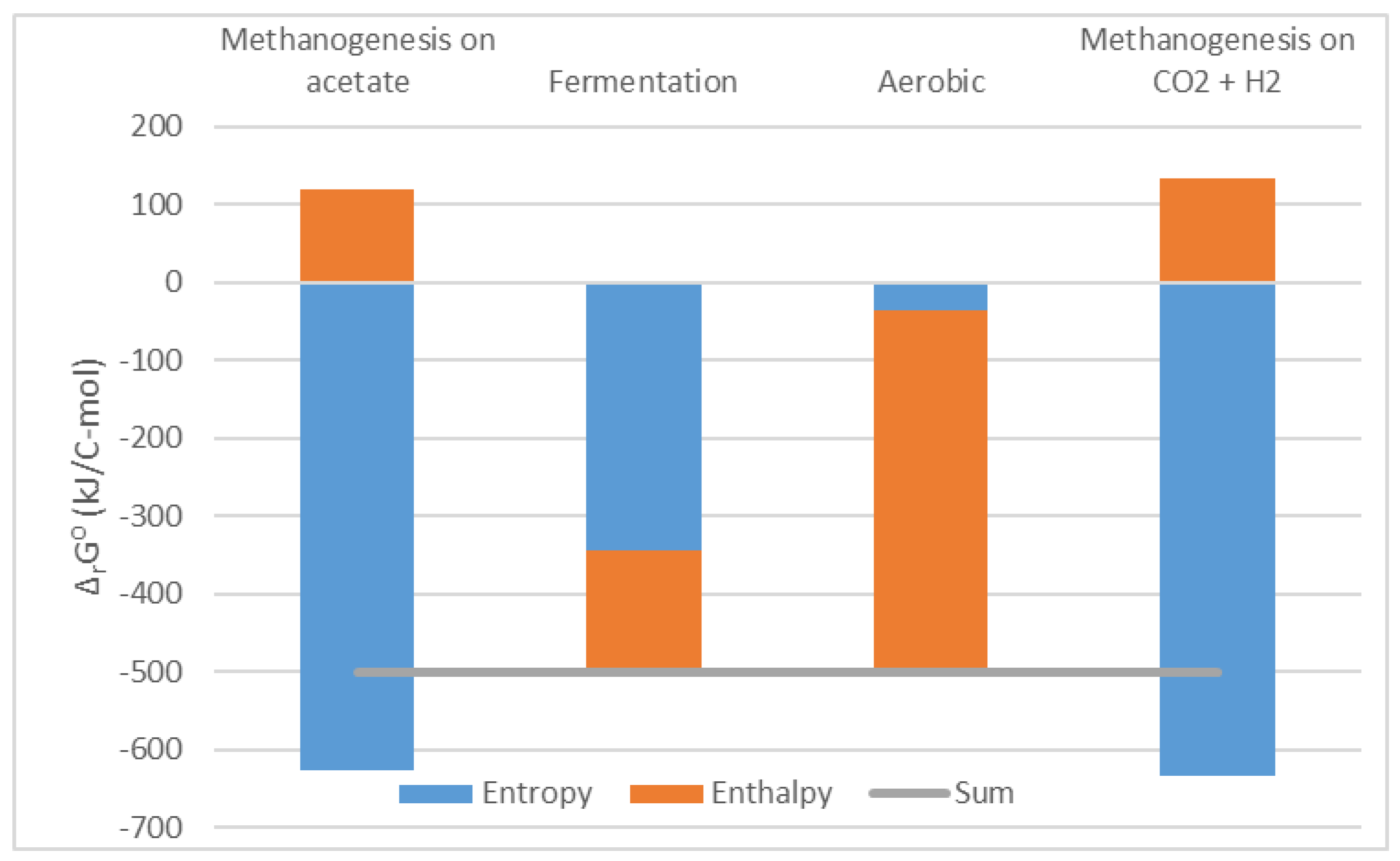
Figure 2.
Comparison of the Monod equation and thermodynamic growth model. The blue circles (●) represent experimental data, the full green line (–––––) a fit with the Monod equation (rmax=1.05 h-1, KS=0.553 mmol/dm³), while the dashed orange line (— ― ―) represents a fit with the thermodynamic growth model (a= 0.2028 h-1, b= 0.6662 h-1) More details can be found in Example 2 (Supplementary Information 1). The experimental data come from (Schulze & Lipe, 1964).
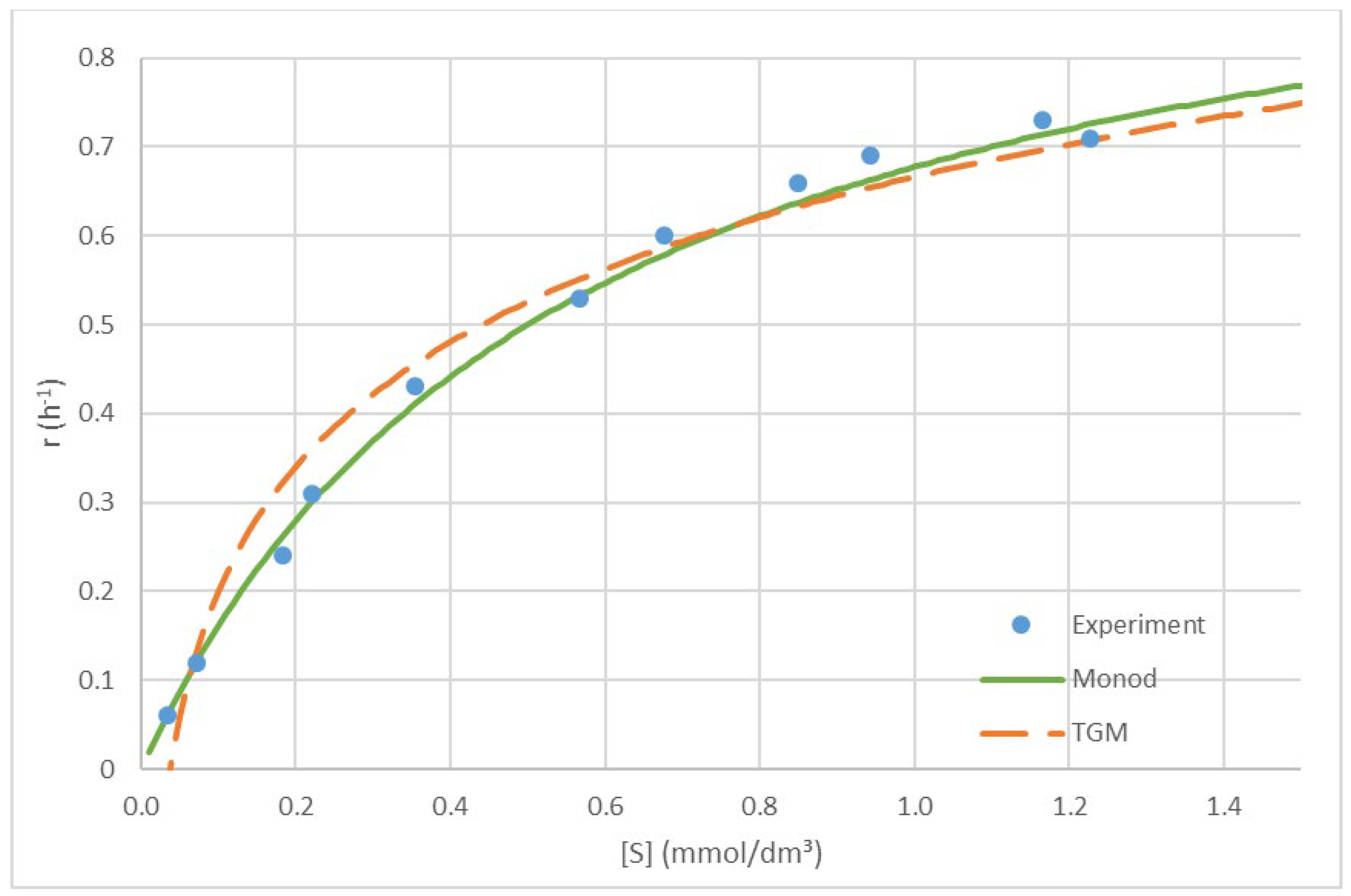
Figure 3.
Fitting the thermodynamic growth model, using a logarithm plot.

Table 1.
Unit carbon formulas and standard thermodynamic properties of some organisms. Data taken from (Popovic, 2019; Popovic & Minceva, 2020c, 2020a).
Table 1.
Unit carbon formulas and standard thermodynamic properties of some organisms. Data taken from (Popovic, 2019; Popovic & Minceva, 2020c, 2020a).
| Organism | Class | Empirical formula | ΔfH⁰ (kJ/C-mol) | Sm⁰ (J/C-mol K) | ΔfG⁰ (kJ/C-mol) |
| Escherichia coli | Bacteria | CH1.770O0.490N0.240 | -114 | 36.4 | -67 |
| Saccharomyces cerevisiae | Yeast | CH1.613O0.557N0.158P0.012S0.003 | -131 | 34.7 | -87 |
| Penicillium chrysogenum | Filamentous fungi | CH1.87O0.22N0.08 | -57 | 29.5 | -19 |
| Chlorella vulgaris | Algae | CH1.667O0.222N0.111 | -51 | 27.6 | -15 |
| Homo sapiens | Human | CH1.730O0.259N0.111P0.013S0.003 | -75 | 29.5 | -38 |
| Poliovirus | Virus | CH1.480O0.394N0.295P0.022S0.007 | -86 | 32.2 | -44 |
Table 2.
The dependence of specific growth rate, r, of E. coli on glucose concentration, [C6H12O6]. Data taken from (Schulze & Lipe, 1964).
Table 2.
The dependence of specific growth rate, r, of E. coli on glucose concentration, [C6H12O6]. Data taken from (Schulze & Lipe, 1964).
| [C6H12O6] (mmol/dm³) | r (h-1) | [C6H12O6] (mmol/ dm³) | r (h-1) | |
| 0.0333 | 0.06 | 0.677 | 0.6 | |
| 0.0722 | 0.12 | 0.849 | 0.66 | |
| 0.1832 | 0.24 | 0.944 | 0.69 | |
| 0.2220 | 0.31 | 1.227 | 0.71 | |
| 0.3552 | 0.43 | 1.166 | 0.73 | |
| 0.5662 | 0.53 |
Table 3.
E. coli growth data transformed for fitting.
| ln[C6H12O6] | r (h-1) | ln[C6H12O6] | r (h-1) | |
| -3.402 | 0.06 | -0.390 | 0.6 | |
| -2.629 | 0.12 | -0.163 | 0.66 | |
| -1.697 | 0.24 | -0.058 | 0.69 | |
| -1.505 | 0.31 | 0.204 | 0.71 | |
| -1.035 | 0.43 | 0.153 | 0.73 | |
| -0.569 | 0.53 |
Disclaimer/Publisher’s Note: The statements, opinions and data contained in all publications are solely those of the individual author(s) and contributor(s) and not of MDPI and/or the editor(s). MDPI and/or the editor(s) disclaim responsibility for any injury to people or property resulting from any ideas, methods, instructions or products referred to in the content. |
© 2023 by the authors. Licensee MDPI, Basel, Switzerland. This article is an open access article distributed under the terms and conditions of the Creative Commons Attribution (CC BY) license (http://creativecommons.org/licenses/by/4.0/).
Copyright: This open access article is published under a Creative Commons CC BY 4.0 license, which permit the free download, distribution, and reuse, provided that the author and preprint are cited in any reuse.


