

Submitted:
19 November 2023
Posted:
20 November 2023
You are already at the latest version
Abstract
Automatic generation control (AGC) plays a vital role in creating an equilibrium between generated output power and load demand, in order to maintain frequency at desired value. This study focuses on performance analysis of simple-multi attribute rating technique (SMART) assisted proportional-integral-derivative (PID) controller design for AGC of two interconnected power systems. PID controller is designed by minimizing frequency variations, area control errors for area-1 and area-2, and tie-line power deviation. An objective function is framed considering error minimization of aforementioned factors as sub-objectives. The construction of objective function involves using the integral of time-multiplied absolute error (ITAE) for frequency deviations for area-1 and area-2, ITAE for deviation in tie-line power, and ITAEs for area control errors for area-1 and area-2 as sub-objective functions. By assigning appropriate weights to these sub-objective functions, an overall objective function is formed. This study determines these weights in an organized manner using SMART method, rather than randomly/equally assigning them. Overall objective function is minimized using Jaya algorithm. To demonstrate effectiveness of the proposed Jaya-based PID controller, its performance is analysed and compared with controllers tuned using other optimization algorithms, including sine cosine, Luus-Jaakola, teacher-learner based optimization, Nelder-Mead simplex, and elephant herding optimization. Considering six different case studies that consider a range of load variations, responses for fluctuations in frequency and tie-line exchange are plotted. Statistical and non-parametric analysis performed further provide additional insights into the performance of Jaya-based PID controller.
Keywords:
AGC
; SMART method
; Jaya optimization
; PID controller
; two-area power system
1. Introduction
Power system operation and control has a fundamental objective of ensuring uninterrupted electricity, of acceptable quality, to all consumers. Due to some abrupt disruptions in power system or any other factors affecting it, sometimes a situation occurs where the generated active power becomes less than the power demand [1,2,3]. This leads to an undesirable deviation in generating units’ frequency and tie-line power. In order to retain the nominal values of frequency and tie-line power, a concept of automatic generation control (AGC) is acknowledged [4,5,6,7]. AGC balances generated output power and load demand, hence maintains frequency and tie-line power exchange [8]. AGC’s primary functions are load frequency control (LFC) and economic dispatch (ED) [9]. The LFC function modifies generating units output for controlling system’s frequency and tie-line power exchange [10]. Distributing load among available generating units in most economical way is responsibility of ED. It is executed by the control center, which ascertains the optimal output for every unit in accordance with its constraints and operational expenses.
An extensive research by several researchers have been performed on AGC for single-area power systems (SAPS) [11,12,13], and multi-area power systems (MAPS) [14,15,16,17]. In [18], authors created a novel control strategy for solving AGC problem in electric power systems by developing a cascaded fuzzy fractional order PI-FOPID (CFFOPI–FOPID) controller. The authors in [19] embarked on an innovative initiative, introducing new hybrid peak-area-based proportional-integral controllers (PICs) for the purpose of optimizing the adjustment of supplementary controller gains. A genetic algorithm (GA) is introduced by authors in [20] to optimize the parameters of PID sliding mode load frequency control in MAPS with nonlinear elements. In [21], a modified version of the traditional automatic generation control loop is integrated to simulate the operation of AGC in a restructured power system.
Excess load demand requirement in SAPS is satisfied by either accelerating generation or by utilizing kinetic energy from rotating machine. However, in MAPS, tie-line power exchange between interconnected power systems satisfies the same requirement. To adjust this tie-line exchange and to nullify frequency deviation, controllers are incorporated in systems. Earlier for AGC, integral controllers were used to control system frequency and tie-line’s power [22]. However, because of their slower time response, researchers used proportional integral (PI) controllers, which are less expensive, simple in structure, and provide a faster time response. Further to improve the dynamic response, they are replaced by proportional integral derivative (PID) controllers.
Tuning of controller parameters is crucial for ensuring reliable and optimal flow of power. For determining the optimal values of controller parameters, there exist three PID tuning methods: heuristic tuning, model-based tuning and rule-based tuning. In recent, heuristic tuning methods are majorly adopted over model-based tuning and rule-based tuning by many researchers [23,24,25,26,27]. This shift is seen due to better tuning obtained with heuristic methods in comparison to model-based tuning and rule-based tuning. While designing a controller, appropriate selection of objective function becomes crucial for better and optimal tuning of parameters. Error indices, such as integral of absolute error (IAE), integral of squared error (ISE), integral of time multiplied absolute error (ITAE), and integral of time multiplied square error (ITSE) are commonly employed to construct objective functions for optimizing controller parameters [28,29,30,31,32,33]. These error indices are utilized in interconnected regions to assess frequency deviations, control errors for area (ACEs), and fluctuations in tie-line power. To construct more appropriate objective function, it is essential to employ a structured technique for ascertaining the corresponding weights of sub-objective criteria.
In this study, a two-area power system (TAPS) is considered in which a PID controller is deployed for AGC. Controller is tuned using Jaya optimization algorithm. A systematic approach known as simple-multi attribute rating technique (SMART) is incorporated for evaluating weights associated with sub-objective functions. For construction of objective function, ITAEs of frequency deviation and control errors, for areas 1 and 2, and ITAE of fluctuation in tie-line power, serve as sub-objective functions. An overall objective function is formed by merging weighted sub-objective functions. Unlike prior literature, this study attempts to ascertain weights of sub-objective functions, in an organized way using SMART method [34], rather than assigning them with equal/random values. To prove applicability of suggested Jaya-based PID controller, its comparisons with controllers, tuned using sine cosine (SC), Luus-Jaakola (LJ), teacher-learner based optimization (TLBO), Nelder-Mead simplex (NMS) and elephant herding optimization (EHO) algorithms, are illustrated in the form of responses and tables. For further validation of work, time domain simulations are performed. These simulations are performed for six distinct case studies with a range of load variations.
The framework of this work is arranged as follows: Section 2 provides a brief introduction of power system along with its control and operation. AGC and its illustration for considered TAPS is discussed in Section 3. The designing of PID controller and construction of objective function is illustrated in Section 4. In Section 5, step wise procedure for determination of weights, using SMART method, is demonstrated. Section 6 exhibits Jaya algorithm. In Section 7, obtained results are displayed and discussed briefly. Derived conclusions of suggested work are commented in Section 8.
2. Power System Operation And Control
2.1. Introduction
Power system serves the purpose of generation, transmission, and distribution of electric power. The architecture of power system necessarily includes networks, generation and distribution, connected by a transmission system [35]. The framework of an electric power system can be presented as:
-
Electrical energy sources:Various energy sources are available in nature that are used for generation of electrical energy. These sources are classified as renewable energy sources, such as water, sun, wind, etc., and non-renewable energy sources, such as nuclear energy, fuels, etc.
-
Generation system:The generation system primarily consists of two components i.e. generator, which generates a high frequency electric power, and transformer, which transmits this high frequency generated power from one voltage level to another voltage level.
-
Transmission system:Transmission system is a network of transmission lines through which electric power is transferred from generation side to distribution side.
-
Distribution system:Distribution system provides power to all consumers of an area from the bulk power sources. This power is delivered to consumers at desired voltage and frequency ratings from distribution system.
2.2. Operation and control
Energy, that is transformed into electricity, is widely employed in transportation, agricultural, commercial, and industrial sectors [36]. Energy in electrical form can be produced and transmitted in large quantities at little cost over great distances [37]. The fundamental objective of power system operation and control is to ensure a consistent and reliable supply of high-quality electricity to all consumers. Equilibrium is achieved when the generation and demand of electricity are in perfect balance. Achieving equilibrium requires the careful balance of both real and reactive power, as AC power encompasses both these components. In recent scenarios, AC systems have surpassed DC systems as the most widely used system for the following reasons:
- 1.
- AC generators are easier to use in comparison to DC generators.
- 2.
- AC voltage level transformation is easier, offering excellent flexibility of various voltage levels during generation, transmission, and distribution.
- 3.
- Commonly used AC motors are easier to operate and more cost-effective than DC motors.
In order to accomplish real power balance (acceptable frequency values) and reactive power balance (acceptable voltage profile), two fundamental control strategies i.e. automatic generation control (AGC) [38] and automatic voltage control (AVR) are used, respectively [39]. This paper deals with balancing of real power values (frequency control) i.e. AGC, which is further discussed in Section 3.
3. Illustration of automatic generation control for considered two area power system
3.1. Automatic generation control
Automatic generation control (AGC) is a crucial component of operation and control of power systems. It plays a major role by maintaining frequency, tie-line power exchange with other systems, and balance between generation and load demand for large-scale interconnected power systems [40]. AGC’s primary goal is to keep the system frequency and tie-line power exchange at the predetermined levels. This is accomplished by modifying the generating units’ output in response to changes in the load demand and system circumstances. Additionally, AGC manages the economic dispatch of generating units, which entails dividing up the load demand among the available units in the most economical manner.
The primary components of AGC includes generating units, communication networks, the control unit, and controllers. The generating units include the renewable and non-renewable sources of power. Exchange of tie-line power and monitoring and controlling of system frequency is managed by control unit. The control unit is connected to controllers via communication networks. Depending on framework of system, the communication network can be wired or wireless. The controllers take control signals as input from control centre for regulating the output of the generating unit.
The basic functions of an AGC system are load frequency control (LFC) and economic dispatch (ED) [41]. The LFC function adjusts output of generating units to control the system frequency and tie-line power exchange [42]. It is categorized into three levels of control: primary, secondary, and tertiary. Primary control is the simplest as well as quickest level of LFC. It is carried out by the governors of the generating units, which change the mechanical power input in response to frequency variations. The next level of LFC is secondary control. It is carried out by the control center, which transmits control signals to controllers in order to rectify frequency deviations and restore tie-line power interchange to their planned values. The last level of LFC is tertiary control. It is also carried out by the control center, which reschedules the output of the generating units in order to optimize system functioning and save fuel costs.
The ED function is responsible for allocating the load demand among the available generating units in the most cost-effective manner [43]. It is carried out by the control center, which determines the best output for each unit based on its operating costs and limits. Depending on the system architecture and requirements, ED can be integrated with LFC or conducted individually.
3.2. Framework of two area power system under consideration
Generally, based on the number of generating and distribution networks, two types of power systems exist i.e. single-area power system (SAPS) and multi-area power system (MAPS). In SAPS, the requirement of higher load demand is fulfilled by machine’s rotating kinetic energy or by accelerating the generation. While in MAPS, the same requirement is met by tie-line power exchange among the interlinked power systems. In this article, a two-area power system (TAPS) is considered from [44], which is illustrated in Figure 1.
The system shown in Figure 1 depicts TAPS, which is an interconnected system comprising two non-reheat thermal power plants, each with 1000 MW nominal load and a combined capacity of 2000 MW. In Figure 1, frequency variations in system are denoted by and . Control errors for area-1 and area-2 are indicated by and , respectively, and and are representing control inputs. Speed regulating constants for governor are depicted by and , while and denote frequency bias factors. and are turbine time constants, and time constants for the power system are denoted by and . Power system gains are represented by and . Governor’s power deviations are depicted by and . Non-reheat steam turbine’s power deviations are denoted by and . And, deviation in interconnected power system’s tie-line power is represented by .
4. Problem Formulation
The goal of AGC is to maintain the dependable and consistent power flow in a multi-area linked power system and reduce frequency variations while meeting system limits [45]. In order to find an optimal solution to these challenges, it is required to formulate a precisely defined objective function. The objective function, along with constraints, will form a basis for tuning of controller. In this article, a proportional-integral-derivative (PID) controller is incorporated. PID controllers just require coefficient tuning, which can be performed manually as well as automatically. This makes their construction simple, and hence they can be implemented very easily [46]. Selecting an appropriate objective function is crucial for optimal operation of power system.
4.1. Design of controller
PID controllers are feedback-based devices that govern a plant, a process, or a system. They function by measuring feedback produced over time and manipulating process’s input as necessary to obtain the desired set-point [47]. Acknowledging recent control design requirements, it has been discovered that a control should limit the influence of load disruptions, avoid excess supply of noise to system, and be resistant to mild changes in process parameters [44]. A schematic diagram of PID controller [48] in shown in Figure 2.
The inputs provided to PID controller are control errors of area-1 and area-2 i.e. and , respectively. and are calculated as:
In (1), is capacity ratio of area-1 to area-2. PID controller includes three controller parameters, namely; proportional gain (), integral gain () and derivative gain (). Fine tuning of these parameters is required to match dynamics of controlled operation. To minimize noise in the signal, a filter (F) along with derivative gain is incorporated. The mathematical representation of PID controller is presented as follows:
Tuning of controller parameters is performed by formulating objective function, which is formulated in following section.
4.2. Construction of objective function
For constructing an objective function, errors in frequency, error in tie-line power, and errors in control areas are considered. This article considers ITAE error minimization [49,50] of frequency variations, tie-line power deviation and area control errors for area-1 and area-2. The objectives to be minimized are considered as , and which are represented as follows:
In (3)-(5), objective, given by (3), denotes ITAE for frequency deviations in area-1 and area-2. Objective, given by (4), depicts ITAE for tie-line power exchange and objective, given by (5), represents ITAE for deviations in control errors for area-1 and area-2. For all objectives, overall time taken for simulation is represented by . Incorporating , and , an overall objective function is formed which is represented as follows:
In (6), , and represent weights corresponding to , and , respectively. These weights decide the significance of their corresponding objective functions in overall objective function . Substituting the values of , and from (3), (4) and (5), respectively, in (6); modifies to:
The values of , and in (7) are determined using a systematic weight determination method. In this article, simple-multi attribute rating technique (SMART) is utilized for weight determination, which is discussed in Section 5. For defining the constraints subjected to overall objective function (7), maximum and minimum values of controller parameters , , and filter coefficient F, are considered. These constraints are mathematically depicted in (8)-(11).
5. SMART method
The simple-multi attribute rating technique (SMART) is a multi attribute decision making (MADM) method which is performed in two phases [51]. In initial phase, the considered attributes are ranked in decreasing order of their significance with respect to their corresponding alternatives. In later phase, attribute having least significance is assigned a minimum performance index. The performance indices range from 10 to 100. Relative relevance of next attribute, in comparison to least significant one, is established by assigning it a performance index greater than the prior one. The attribute with performance index 100 is identified as most significant one, whereas one with performance index 10 denotes the least importance. Further, based on performance indices, the score and cumulative score for each alternative are computed to obtain normalized cumulative score [52]. This normalized cumulative score determines the optimal weight distribution across alternatives.
In this work, objective functions , and are identified as “alternatives” while, frequency deviations in area-1 and area-2, and deviation in tie line power are identified as “attributes”. These attributes are represented as , and , respectively. The procedure for determining weights incorporated in overall objective function (7), using SMART method, is provided below.
Step 1: A decision matrix is constructed by providing a significance level to each attribute with respect to alternatives. The constructed decision matrix is provided in Table 1.
Step 2: Based on importance level given to each attribute for all alternatives, performance indices are provided. Minimum index value is considered as 10 while maximum index value is considered as 100. So Table 1 is further modified by incorporating performance indices, and modified version is shown as Table 2.
Step 3: After allocating performance indices to attributes, score for each alternative is calculated. The scores are calculated as
where, depicts score and denotes performance index. and are considered as 10 and 100, respectively. The calculated scores are tabulated in Table 3.
Step 4: After obtaining scores, cumulative scores are required to be calculated. For computing cumulative scores, initially performance indices are multiplied to their corresponding attribute’s importance factor. For , and , the importance factors are 0.4, 0.3 and 0.3, respectively. Then for each alternative, the modified performance indices are summed up to obtain cumulative score. The modified performance indices along with cumulative scores are tabulated in Table 4.
Step 5: In final step, weights are calculated by normalizing cumulative scores obtained in Table 4. The normalization of cumulative scores is obtained using (13).
In (13), and denote cumulative score and normalized cumulative score for weight. The obtained normalized cumulative scores for , and are tabulated in Table 5.
6. Jaya Algorithm
The Jaya algorithm was originally developed to address unconstrained optimization problems as well as constrained ones [53,54]. In Sanskrit, the term “Jaya” signifies “victory” which becomes the base idea for this algorithm. It takes inspiration from the natural concept of “survival of the best”. The solutions within the Jaya population are drawn towards global optimal solution while simultaneously disregarding the least fitting solution. This algorithm does not require any algorithm-specific controlling parameter and just relies on overall number of iterations and size of population.
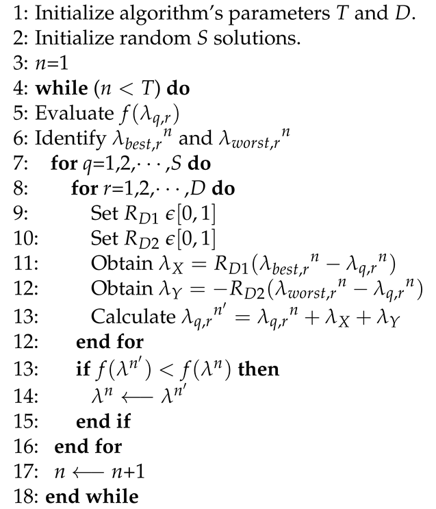
Let the overall number of iterations be denoted by T. The total number of decision parameters is D and population size is given as S. The decisions parameters are denoted by where, and . Suppose worst and best solutions obtained at any iteration are given as and , respectively. For iteration, updated value of decision parameter, for solution among the population S, is given as follows:
where,
In (17), and are random numbers in range of zero to unity. At termination stage of every iteration, an updated value is obtained. This value is utilised for next iteration only if it is better than current value .
Jaya algorithm is implemented to minimize overall objective function (15) subjected to constraints (8)-(11) in this article. Its implementation steps are presented in form of a pseudo-code as shown in Algorithm 1.
| Algorithm 1 Pseudo-code for Jaya algorithm |
 |
7. Results And Discussions
The AGC problem for two-area power system (TAPS), illustrated in Figure 1, is scrutinized in this section. Three different objectives are merged into a single objective function (15), whose weights are determined employing SMART method. Constraints subjected to (15) are depicted in (8)-(11). For verifying the applicability of work, simulations for time domain are performed, considering six distinct case studies with a range of load variations. These case studies are tabulated in Table 6.
For each case, objective function (15) is minimized using Jaya, SCA, LJ, TLBO, NMS and EHO algorithms. The optimal values obtained for objective (), sub-objective functions (, , ) and decision parameters (, , and F) evaluated for optimal values of (, , , ), are tabulated in Table 7, Table 8, Table 9, Table 10, Table 11 and Table 12, for case-study I to case-study VI, respectively. Time domain specifications (TDS) of fluctuations in tie-line power and frequency for area-1 and area-2, are also presented in Table 7, Table 8, Table 9, Table 10, Table 11 and Table 12. In this work, considered TDS are peak overshoot and settling time.
A comparative analysis is performed for comparing performances of controllers tuned using Jaya, SCA, LJ, TLBO, NMS and EHO algorithms. For each of the six case studies mentioned in Table 6, above mentioned optimization algorithms are executed 50 times in a sequence. The outcomes of this comparative analysis are tabulated in Table 13.
For case-study I, the outcomes are tabulated in Table 7. For visual representation of fluctuations in frequency for area-1 () and area-2 () and fluctuations in tie-line power (), their responses are shown in Figure 3, Figure 4, and Figure 5, respectively. From Table 7, it can be seen that Jaya-based PID controller settles fastest among all the other algorithms-based PID controllers. Even the most optimum i.e minimum value of objective function is achieved by Jaya-based PID controller. Similarly, values of sub-objective functions , , and are also minimum in case of Jaya-based PID controller.
The results for case-study II are presented in Table 8. The responses are displayed in Figure 6, Figure 7, and Figure 8, to provide a visual depiction of , and , respectively. Table 8 shows that Jaya-based PID controller settles the fastest out of all the PID controllers. The Jaya-based PID controller even attains the minimal value of the objective function , which is the most optimal. In case of Jaya-based PID controller, minimum values of sub-objective functions , , and are also attained.
Table 9 summarizes the outcomes of case-study III. Visual representations of response variations for , and can be observed in Figure 9, Figure 10, and Figure 11, respectively. Table 9 highlights that Jaya-based PID controller exhibits the least settling time among all the PID controllers utilizing different algorithms. Additionally, the Jaya-based PID controller achieves the lowest value for the optimal objective function, and also for sub-objective functions , , and .
For case-study IV, the results obtained are presented in Table 10. Response of is shown in Figure 12, is depicted in Figure 13 and is illustrated in Figure 14. Similar to previous cases, for this case also, it is observed that obtained settling time is least for Jaya-based algorithm. Also the least values for , , , and are also observed for Jaya-based PID controller among others.
Table 11 presents the results for case study V. To visually represent , , and , the corresponding responses are depicted in Figure 15, Figure 16, and Figure 17, respectively. Table 11 illustrates that Jaya-based PID controller exhibits the shortest settling time among the PID controllers based on different algorithms. Furthermore, it achieves the lowest value for the objective function and, sub-objective functions , , and .
The outcomes of case-study VI are presented in Table 12. Visual depictions of variations in responses for , , and can be observed in Figure 18, Figure 19, and Figure 20, respectively. From Table 12, it is evident that Jaya-based PID controller demonstrates the least settling time among all the PID controllers employing different algorithms. Moreover, even for this case, the Jaya-based PID controller attains the lowest values for the objective function, , as well as for the sub-objective functions , , and .
A comparative statistical analysis for Jaya, SCA, LJ, TLBO, NMS and EHO based algorithms, for all six case studies considered in Table 6, is performed. The findings of this analysis are tabulated in Table 13. The statistical measures considered for analysis are mean value, minimum value, maximum value, and standard deviations. While comparing the outcomes of all algorithms from Table 13, it is observed that Jaya algorithm based controller performed the best among Jaya, SCA, LJ, TLBO, NMS and EHO algorithms, giving the least mean and minimum values among all the algorithms, for case study I, case study II, case study III, case study IV, case study V and case study VI. Also the standard deviations obtained by Jaya algorithm are least for all six case studies. Hence, this comparative analysis proves the superiority in performance of Jaya-based PID controller over other considered algorithms.
For non-parametric analysis, a Friedman rank test is performed to compare the performances of optimization based on Jaya, SCA, LJ, TLBO, NMS and EHO algorithms. In this test, overall Q value and p value for all algorithms and mean rank for each algorithm, are evaluated. Performance of algorithm holding least mean rank is considered as best among all algorithms. For validation of this test, Q value should be positive and p value should be less than 5%. In Table 14, mean ranks for all the above mentioned algorithms, along with overall Q value and p value, are provided. The mean ranks for Jaya, SCA, LJ, TLBO, NMS and EHO algorithms are 1, 4.6666, 4.6666, 4, 3.5 and 3.1666, respectively. From these values, it is noticed that Jaya optimization algorithm yields best results than other as it holds mean rank 1. Q value obtained is 16 which is positive value and p value is 0.006844 which is much lesser than 0.05. Hence, it can be concluded that Jaya-based PID controller outperforms others.
8. Conclusion
This article focused on evaluating the performance of SMART method assisted PID controller designed for AGC. PID controller is designed on the basis of an objective function formulated by merging three sub-objective functions, each for minimizing frequency variations, area control errors in both area-1 and area-2, and tie-line power deviations, respectively. The weights associated with these sub-objective functions are determined using SMART method. The optimization of overall objective function is performed using the Jaya algorithm. The effectiveness of the proposed Jaya-based PID controller is assessed by comparing its performance with sine cosine (SC), Luus-Jaakola (LJ), teacher-learner based optimization (TLBO), Nelder-Mead simplex (NMS), and elephant herding optimization (EHO) algorithm based PID controllers. Six different case scenarios with varying load conditions are considered. The results obtained from simulations indicate that more optimal values are executed by Jaya-based PID controller than others. Responses for fluctuations in frequency and tie-line power exchange, obtained for all algorithm-based PID controllers, for each case, are plotted. From responses, it is clear that least deviations are achieved by Jaya-based PID controller, signifying its superiority over others. For further validation of overall performance and applicability of suggested controller, statistical as well as non-parametric analysis are also performed, for all cases.
Author Contributions
Conceptualization, V. P. S., A. V. W., V. P. M.; methodology, A. V. W., U. K. Y., V. P. S.; software, V. P. S., A. V. W., V. P. M.; validation, V. P. S, A. V. W., T. V.; formal analysis, A. V. W., V. P. S, U. K. Y.; investigation, A. V. W., V. P. S, T. V.; resources, V. P. S., A. V. W., V. P. M.; data curation, V. P. S., A. V. W., V. P. M.; writing—original draft preparation, V. P. S., A. V. W., V. P. M.; writing—review and editing, V. P. S., A. V. W., V. P. M.
Funding
The author(s) received no financial support for the research, authorship, and/or publication of this article.
Data Availability Statement
The authors declare no associated data in the manuscript.
Conflicts of Interest
The authors declare no competing interests.
Appendices
| Appendix A: Parameters of two-area interconnected power system | |
| Frequency | Hz; |
| Frequency bias factors | , p.u. Mw/Hz; |
| Speed regulating constants for governors | , Hz/p.u.; |
| Time constants for turbine | , s; |
| System gains | , Hz/p.u. Mw; |
| Torque co-efficient for synchronization | p.u.; |
| Area-1 to area-2 tie-line ratio | . |
| Appendix B: Constraints for controller parameters | |
| Filter gain | ; . |
| Integral gain | ; ; |
| Proportional gain | ; ; |
| Derivative gain | ; ; |
References
- Ullah, K.; Basit, A.; Ullah, Z.; Albogamy, F.R.; Hafeez, G. Automatic generation control in modern power systems with wind power and electric vehicles. Energies 2022, 15, 1771. [Google Scholar] [CrossRef]
- Liu, X.; Qiao, S.; Liu, Z. A survey on load frequency control of multi-area power systems: Recent challenges and Strategies. Energies 2023, 16, 2323. [Google Scholar] [CrossRef]
- Sahu, R.K.; Gorripotu, T.S.; Panda, S. Automatic generation control of multi-area power systems with diverse energy sources using teaching learning based optimization algorithm. Engineering Science and Technology, an International Journal 2016, 19, 113–134. [Google Scholar] [CrossRef]
- Al-Majidi, S.D.; Altai, H.D.S.; Lazim, M.H.; Al-Nussairi, M.K.; Abbod, M.F.; Al-Raweshidy, H.S. Bacterial Foraging Algorithm for a Neural Network Learning Improvement in an Automatic Generation Controller. Energies 2023, 16, 2802. [Google Scholar] [CrossRef]
- Kumar, P.; Kothari, D.P.; others. Recent philosophies of automatic generation control strategies in power systems. IEEE transactions on power systems 2005, 20, 346–357. [Google Scholar]
- Rout, U.K.; Sahu, R.K.; Panda, S. Design and analysis of differential evolution algorithm based automatic generation control for interconnected power system. Ain Shams Engineering Journal 2013, 4, 409–421. [Google Scholar] [CrossRef]
- Chown, G.A.; Hartman, R.C. Design and experience with a fuzzy logic controller for automatic generation control (AGC). IEEE Transactions on power systems 1998, 13, 965–970. [Google Scholar] [CrossRef]
- Bevrani, H.; Hiyama, T. Intelligent automatic generation control. CRC press, 2017. [Google Scholar]
- Golpira, H.; Bevrani, H. Application of GA optimization for automatic generation control design in an interconnected power system. Energy Conversion and Management 2011, 52, 2247–2255. [Google Scholar] [CrossRef]
- Iracleous, D.; Alexandridis, A. A multi-task automatic generation control for power regulation. Electric Power Systems Research 2005, 73, 275–285. [Google Scholar] [CrossRef]
- Ramakrishna, K.; Bhatti, T. Automatic generation control of single area power system with multi-source power generation. Proceedings of the Institution of Mechanical Engineers, Part A: Journal of Power and Energy 2008, 222, 1–11. [Google Scholar] [CrossRef]
- Hossaiin, M.; Takahashi, T.; Rabbani, M.; Sheikh, M.; Anower, M. Fuzzy-proportional integral controller for an AGC in a single area power system. 2006 International Conference on Electrical and Computer Engineering. IEEE; 2006; pp. 120–123. [Google Scholar]
- Dabur, P.; Yadav, N.K.; Avtar, R. Matlab design and simulation of AGC and AVR for single area power system with fuzzy logic control. International Journal of Soft Computing and Engineering 2012, 1, 44–49. [Google Scholar]
- Temiz, A.; Guven, A.N. An AGC Algorithm for Multi-Area Power Systems in Network Splitting Conditions. 2023 IEEE PES GTD International Conference and Exposition (GTD). IEEE; 2023; pp. 77–81. [Google Scholar]
- Salim, N.; Zambri, N.A. Automatic Generation Control System: The Impact of Battery Energy Storage in Multi Area Network. International Journal of Integrated Engineering 2023, 15, 208–216. [Google Scholar] [CrossRef]
- Khan, I.A.; Mokhlis, H.; Mansor, N.N.; Illias, H.A.; Usama, M.; Daraz, A.; Wang, L.; Awalin, L.J. Load Frequency Control using Golden Eagle Optimization for Multi-Area Power System Connected Through AC/HVDC Transmission and Supported with Hybrid Energy Storage Devices. IEEE Access 2023. [Google Scholar] [CrossRef]
- Shouran, M.; Anayi, F.; Packianather, M.; Habil, M. Different fuzzy control configurations tuned by the bees algorithm for LFC of two-area power system. Energies 2022, 15, 657. [Google Scholar] [CrossRef]
- Arya, Y. A novel CFFOPI-FOPID controller for AGC performance enhancement of single and multi-area electric power systems. ISA transactions 2020, 100, 126–135. [Google Scholar] [CrossRef]
- Pathak, N.; Bhatti, T.; Verma, A.; Nasiruddin, I. AGC of two area power system based on different power output control strategies of thermal power generation. IEEE Transactions on Power Systems 2017, 33, 2040–2052. [Google Scholar] [CrossRef]
- Pingkang, L.; Hengjun, Z.; Yuyun, L. Genetic algorithm optimization for AGC of multi-area power systems. 2002 IEEE Region 10 Conference on Computers, Communications, Control and Power Engineering. TENCOM’02. Proceedings. IEEE; 2002; 3, pp. 1818–1821. [Google Scholar]
- Bhatt, P.; Roy, R.; Ghoshal, S. Optimized multi area AGC simulation in restructured power systems. International Journal of Electrical Power & Energy Systems 2010, 32, 311–322. [Google Scholar]
- Daraz, A.; Malik, S.A.; Haq, I.U.; Khan, K.B.; Laghari, G.F.; Zafar, F. Modified PID controller for automatic generation control of multi-source interconnected power system using fitness dependent optimizer algorithm. PloS one 2020, 15, e0242428. [Google Scholar] [CrossRef]
- Zafar, M.H.; Khan, N.M.; Mansoor, M.; Sanfilippo, F. Optimal Tuning of PID Controller for Boost Converter using Meta-Heuristic Algorithm for Renewable Energy Applications.
- Rajeshwaran, S.; Kumar, C.; Ganapathy, K. Hybrid Optimization Based PID Controller Design for Unstable System. Intelligent Automation & Soft Computing 2023, 35. [Google Scholar]
- Azegmout, M.; Mjahed, M.; El Kari, A.; Ayad, H. New Meta-heuristic-Based Approach for Identification and Control of Stable and Unstable Systems. INTERNATIONAL JOURNAL OF COMPUTERS COMMUNICATIONS & CONTROL 2023, 18. [Google Scholar]
- Alahakoon, S.; Roy, R.B.; Arachchillage, S.J. Optimizing Load Frequency Control in Standalone Marine Microgrids Using Meta-Heuristic Techniques. Energies 2023, 16, 4846. [Google Scholar] [CrossRef]
- Mishra, D.P.; Raut, U.; Gaur, A.P.; Swain, S.; Chauhan, S. Particle Swarm Optimization and Genetic Algorithms for PID Controller Tuning. 2023 5th International Conference on Smart Systems and Inventive Technology (ICSSIT). IEEE, 2023, pp. 189–194.
- Duarte-Forero, J.; Obregón-Quiñones, L.; Valencia-Ochoa, G. Comparative analysis of intelligence optimization algorithms in the thermo-economic performance of an energy recovery system based on organic rankine cycle. Journal of Energy Resources Technology 2021, 143, 112101. [Google Scholar] [CrossRef]
- Soni, Y.K.; Bhatt, R. BF-PSO optimized PID controller design using ISE, IAE, IATE and MSE error criteria. International Journal of Advanced Research in Computer Engineering & Technology (IJARCET) 2013, 2, 2333–2336. [Google Scholar]
- Abdel-Halim, H.A.; Othman, E.; Sakr, A.; Zaki, A.; Abouelsoud, A. A Comparative Study of Intelligent Control System Tuning Methods for an Evaporator based on Genetic Algorithm. International Journal of Applied Information Systems 2017, 11, 1–14. [Google Scholar] [CrossRef]
- Surjan, R. Design of fixed structure optimal robust controller using genetic algorithm and particle swarm optimization. Int. J. Engineering and Advanced Technology 2012, 2, 187–190. [Google Scholar]
- Zahir, A.M.; Alhady, S.S.N.; Wahab, A.; Ahmad, M. Objective functions modification of GA optimized PID controller for brushed DC motor. International Journal of Electrical and Computer Engineering 2020, 10, 2426. [Google Scholar] [CrossRef]
- Mousakazemi, S.M.H. Comparison of the error-integral performance indexes in a GA-tuned PID controlling system of a PWR-type nuclear reactor point-kinetics model. Progress in Nuclear Energy 2021, 132, 103604. [Google Scholar] [CrossRef]
- Dwanoko, Y.; Habibi, F.; Purwanto, H.; Swastika, I.; Hudha, M. The smart method to support a decision based on multi attributes identification. IOP Conference Series: Materials Science and Engineering. IOP Conference Series: Materials Science and Engineering 2018, 434, 012037. [Google Scholar] [CrossRef]
- Gonen, T. Modern power system analysis; CRC Press, 2013.
- Chakrabarti, A.; Halder, S. Power system analysis: operation and control; PHI Learning Pvt. Ltd., 2022.
- Sivanagaraju, S. Power system operation and control; Pearson Education India, 2009.
- Ali, A.; Biru, G.; Banteyirga, B. Fuzzy Logic-Based AGC and AVR for Four-Area Interconnected Hydro Power System. Electric Power Systems Research 2023, 224, 109494. [Google Scholar] [CrossRef]
- Kumal, S.; others. AGC and AVR of Interconnected Thermal Power System while considering the effect of GRC’s. Int. J. Soft Comput. Eng.(IJSCE) 2012, 2, 2117–2126. [Google Scholar]
- Masrur, H.; Ferdoush, A.; Rabbani, M.G. Automatic Generation Control of two area power system with optimized gain parameters. 2015 International Conference on Electrical Engineering and Information Communication Technology (ICEEICT), 2015, pp. 1–5. [CrossRef]
- Gopi, P.; Reddy, P.L. A Critical review on AGC strategies in interconnected power system. IET Chennai fourth international conference on sustainable energy and intelligent systems (SEISCON 2013). IET, 2013, pp. 85–92.
- Karnavas, Y.; Papadopoulos, D. AGC for autonomous power system using combined intelligent techniques. Electric power systems research 2002, 62, 225–239. [Google Scholar] [CrossRef]
- Al-Awami, A.T. Control-based Economic Dispatch Augmented by AGC for Operating Renewable-rich Power Grids. 2019 IEEE 10th GCC Conference & Exhibition (GCC). IEEE, 2019, pp. 1–5.
- Krishna, P.J.; Meena, V.P.; Singh, V.P.; Khan, B. Rank-Sum-Weight Method Based Systematic Determination of Weights for Controller Tuning for Automatic Generation Control. IEEE Access 2022, 10, 68161–68174. [Google Scholar] [CrossRef]
- Debs, A.S. Automatic Generation Control. In Modern Power Systems Control and Operation; Springer US: Boston, MA, 1988; pp. 203–237. [Google Scholar] [CrossRef]
- Oonsivilai, A.; Marungsri, B. Optimal PID tuning for AGC system using adaptive Tabu search. ACE 2007, 1, 2. [Google Scholar]
- Mohapatra, T.K.; Sahu, B.K. Design and implementation of SSA based fractional order PID controller for automatic generation control of a multi-area, multi-source interconnected power system. 2018 Technologies for Smart-City Energy Security and Power (ICSESP). IEEE, 2018, pp. 1–6.
- Krishna, P.; Meena, V.; Singh, V.; Khan, B. Rank-sum-weight method based systematic determination of weights for controller tuning for automatic generation control. IEEE Access 2022, 10, 68161–68174. [Google Scholar] [CrossRef]
- Awouda, A.E.A.; Mamat, R.B. Refine PID tuning rule using ITAE criteria. 2010 The 2nd International conference on computer and automation engineering (ICCAE). IEEE, 2010, Vol. 5, pp. 171–176.
- Chen, G.; Li, Z.; Zhang, Z.; Li, S. An improved ACO algorithm optimized fuzzy PID controller for load frequency control in multi area interconnected power systems. IEEE Access 2019, 8, 6429–6447. [Google Scholar] [CrossRef]
- Alinezhad, A.; Khalili, J.; Alinezhad, A.; Khalili, J. SMART method. New methods and applications in multiple attribute decision making (MADM). 2019, pp. 1–7.
- Fahlepi, R. Decision support systems employee discipline identification using the simple multi attribute rating technique (smart) method. Journal of Applied Engineering and Technological Science (JAETS) 2020, 1, 103–112. [Google Scholar] [CrossRef]
- Rao, R. Jaya: A simple and new optimization algorithm for solving constrained and unconstrained optimization problems. International Journal of Industrial Engineering Computations 2016, 7, 19–34. [Google Scholar]
- Houssein, E.H.; Gad, A.G.; Wazery, Y.M. Jaya algorithm and applications: A comprehensive review. Metaheuristics and Optimization in Computer and Electrical Engineering 2021, 3–24. [Google Scholar]
Figure 1.
Representation of TAPS.
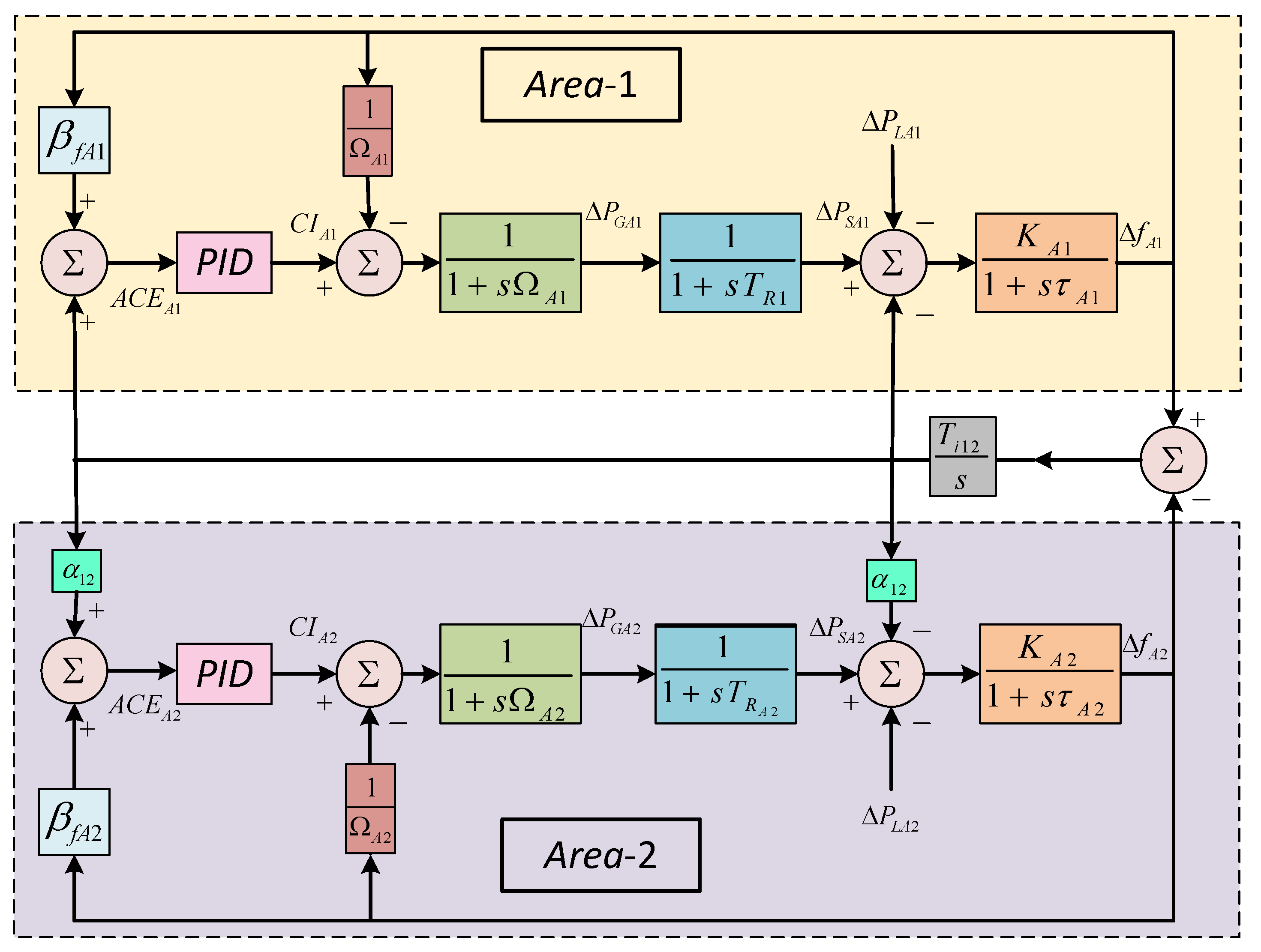
Figure 2.
Representation of PID controller with derivative gain filter
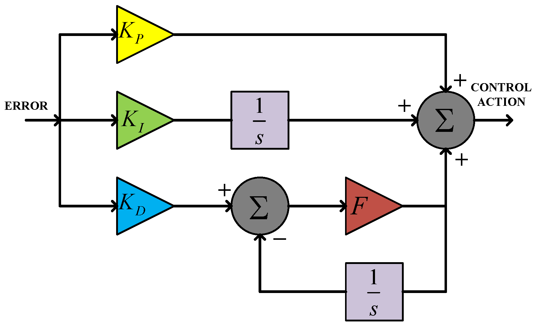
Figure 3.
Case I: Frequency fluctuations for area-1.
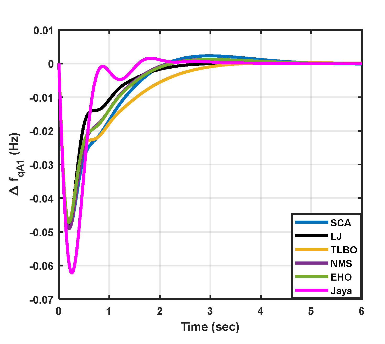
Figure 4.
Case I: Frequency fluctuations for area-2.
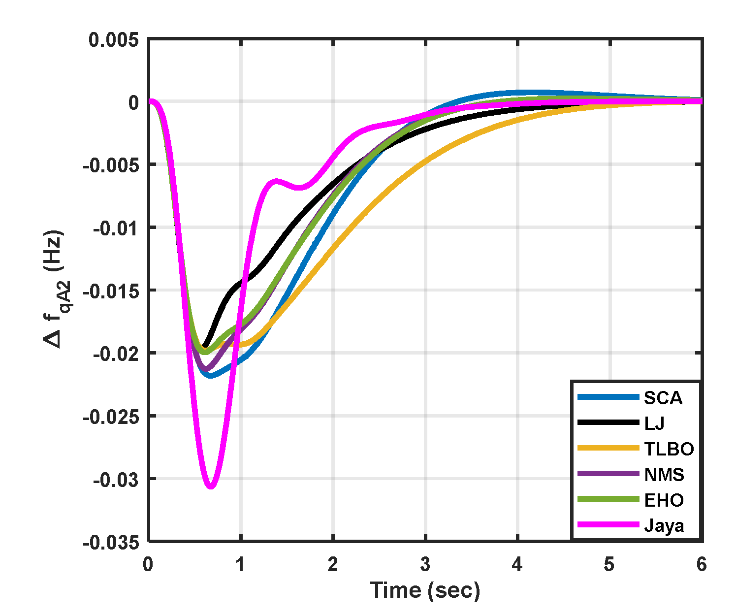
Figure 5.
Case I: Tie-line power fluctuation.
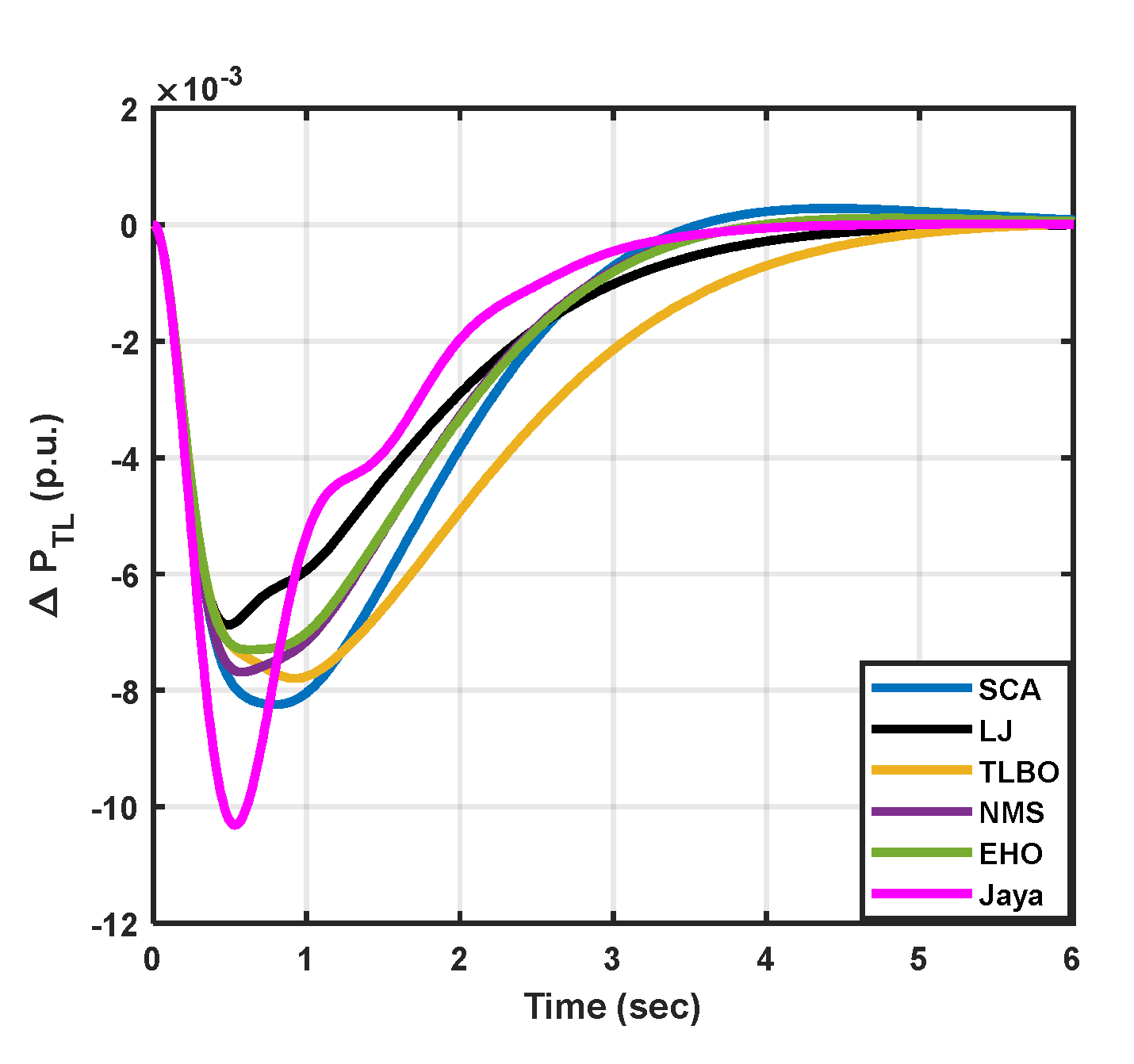
Figure 6.
Case II: Frequency fluctuation for area-1.
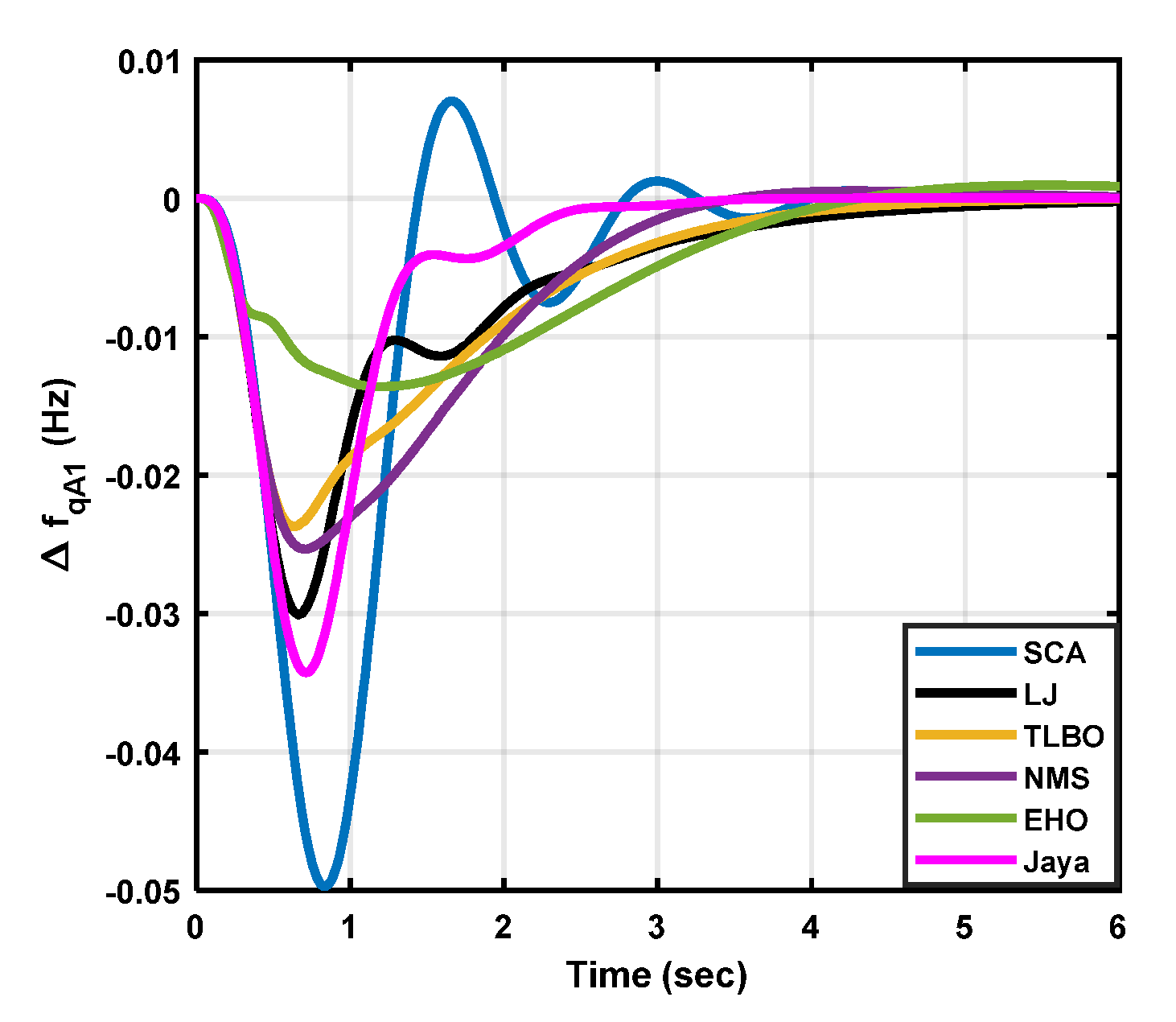
Figure 7.
Case II: Frequency fluctuation for area-2.
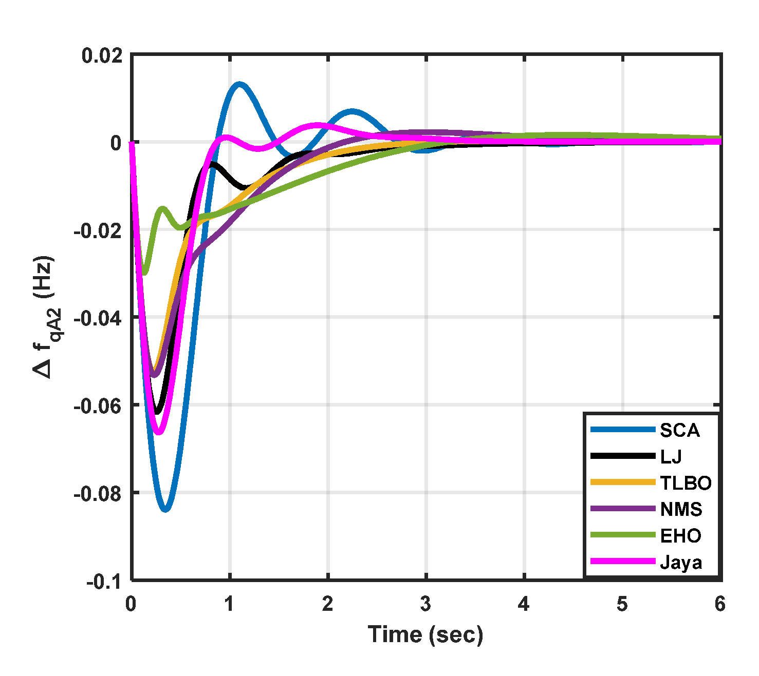
Figure 8.
Case II: Tie-line power fluctuation
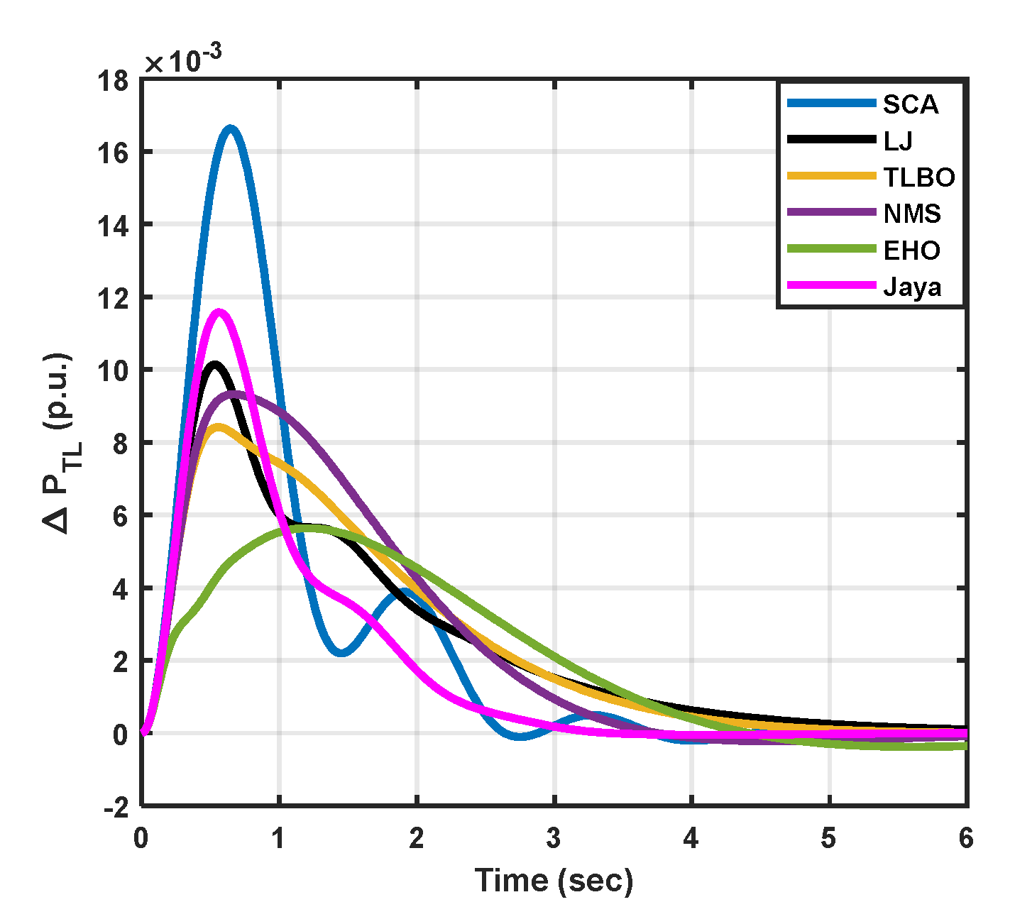
Figure 9.
Case III: Frequency fluctuation for area-1.
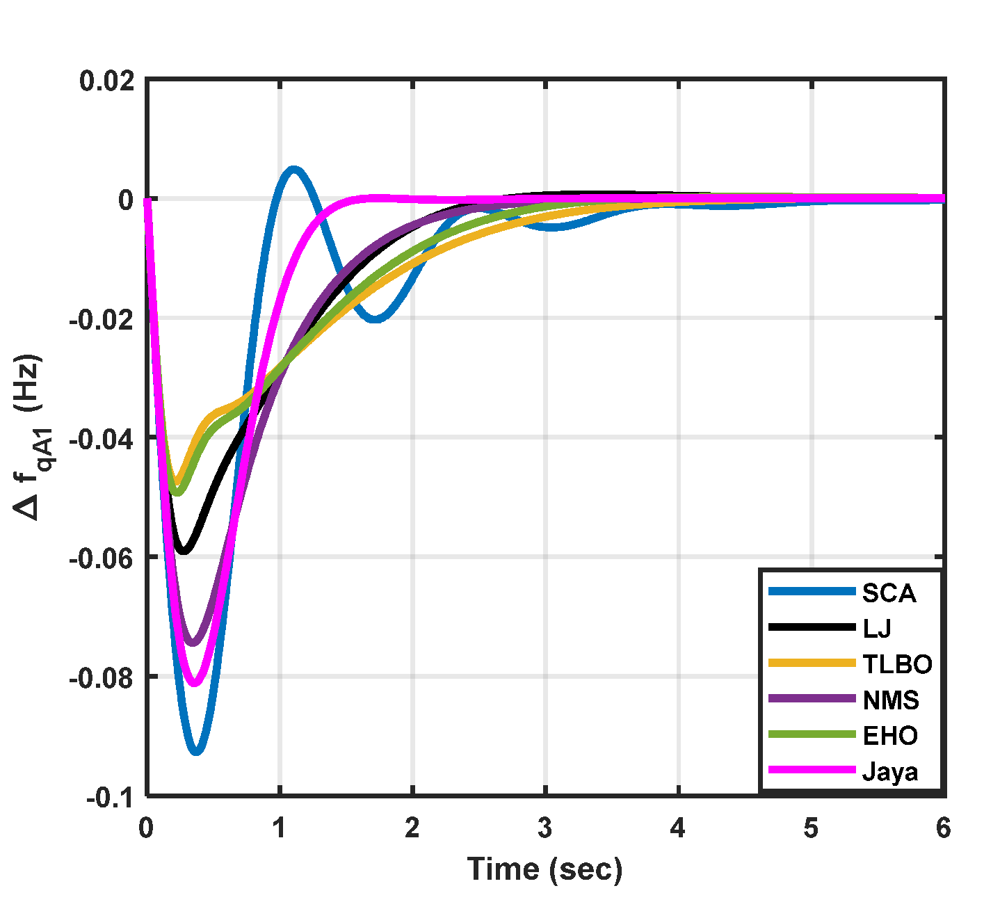
Figure 10.
Case III: Frequency fluctuation for area-2.
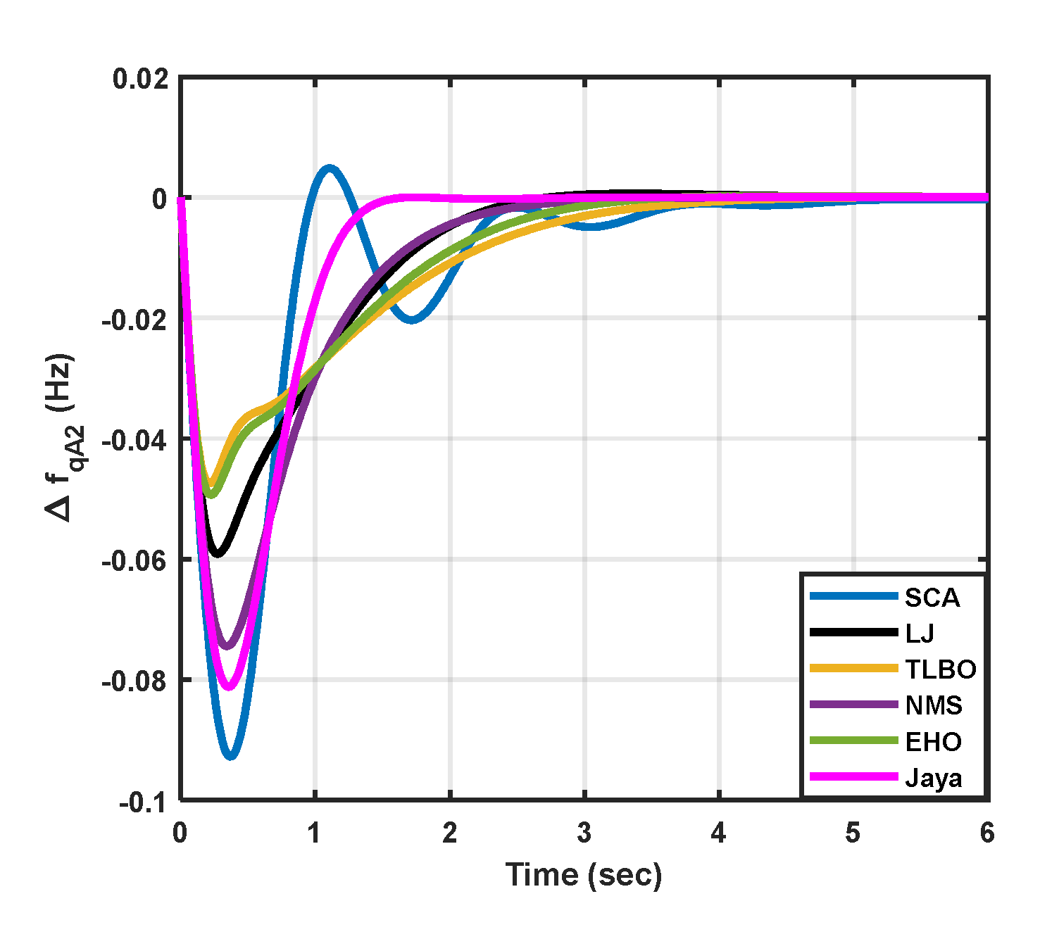
Figure 11.
Case III: Tie-line power fluctuation.
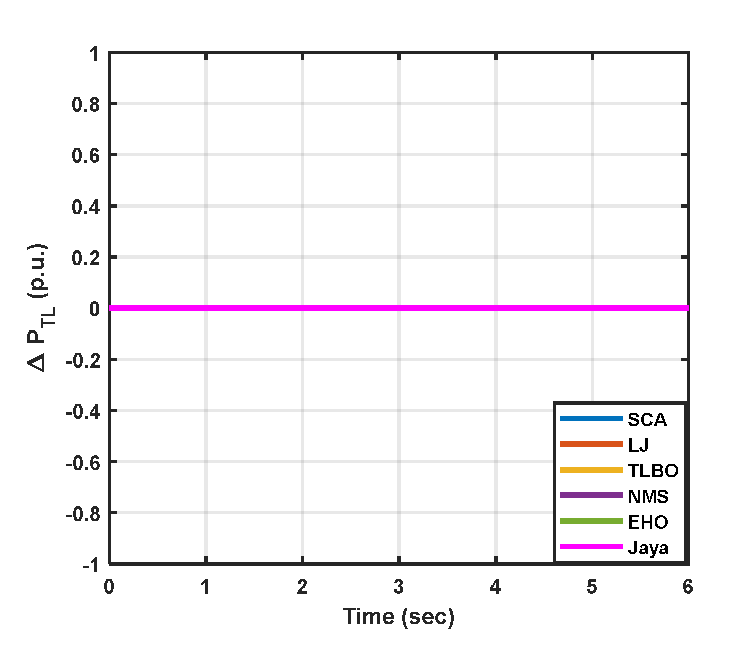
Figure 12.
Case IV: Frequency fluctuations for area-1.
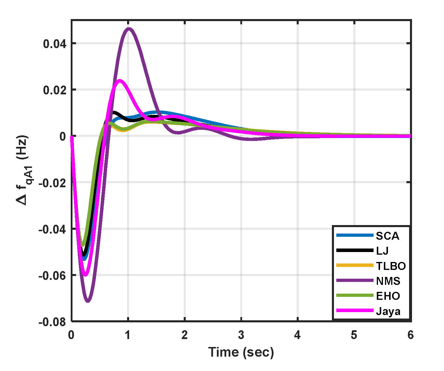
Figure 13.
Case IV: Frequency fluctuations for area-2.
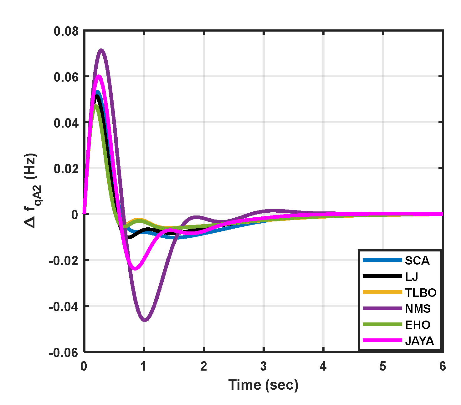
Figure 14.
Case IV: Tie-line power fluctuation.
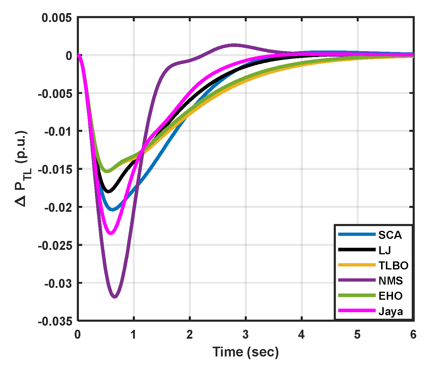
Figure 15.
Case V: Frequency fluctuations for area-1.
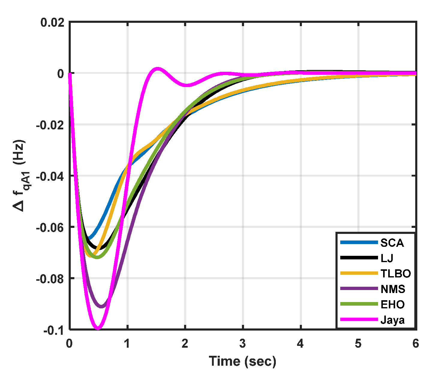
Figure 16.
Case V: Frequency fluctuations for area-2.
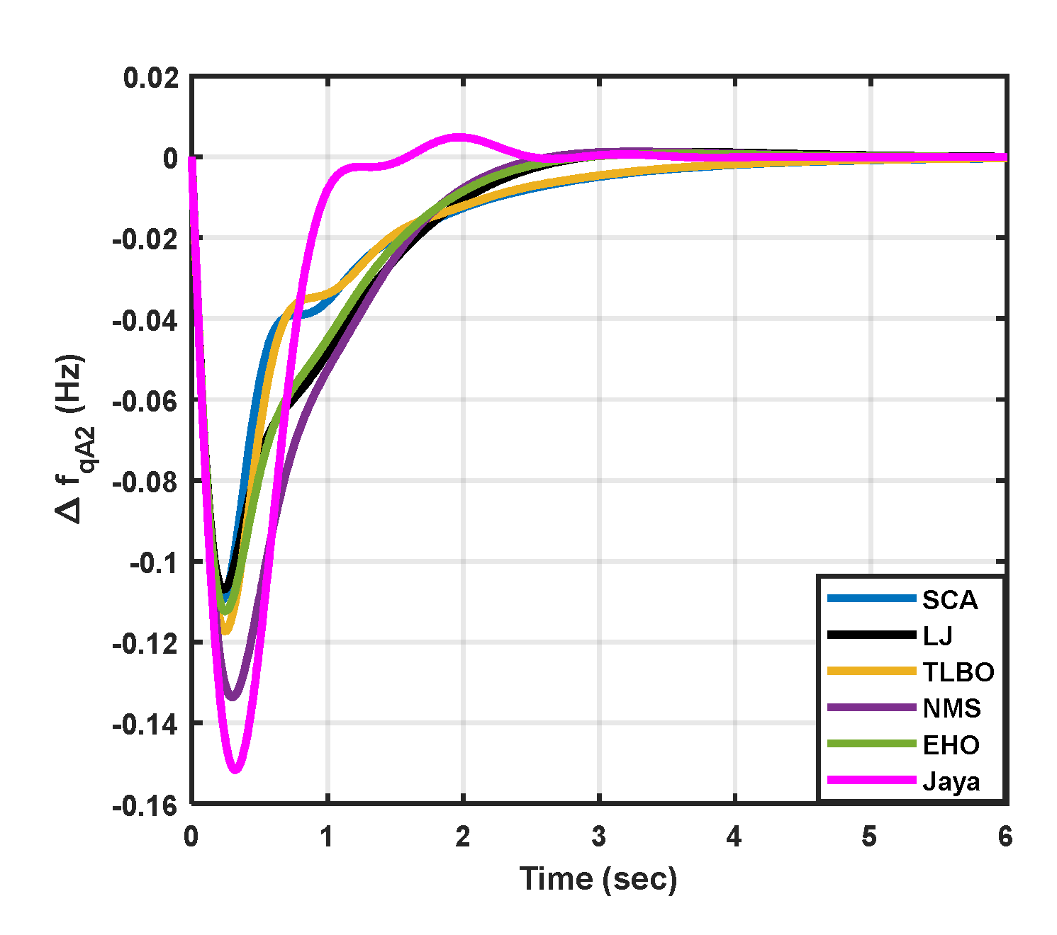
Figure 17.
Case V: Tie-line power fluctuation.
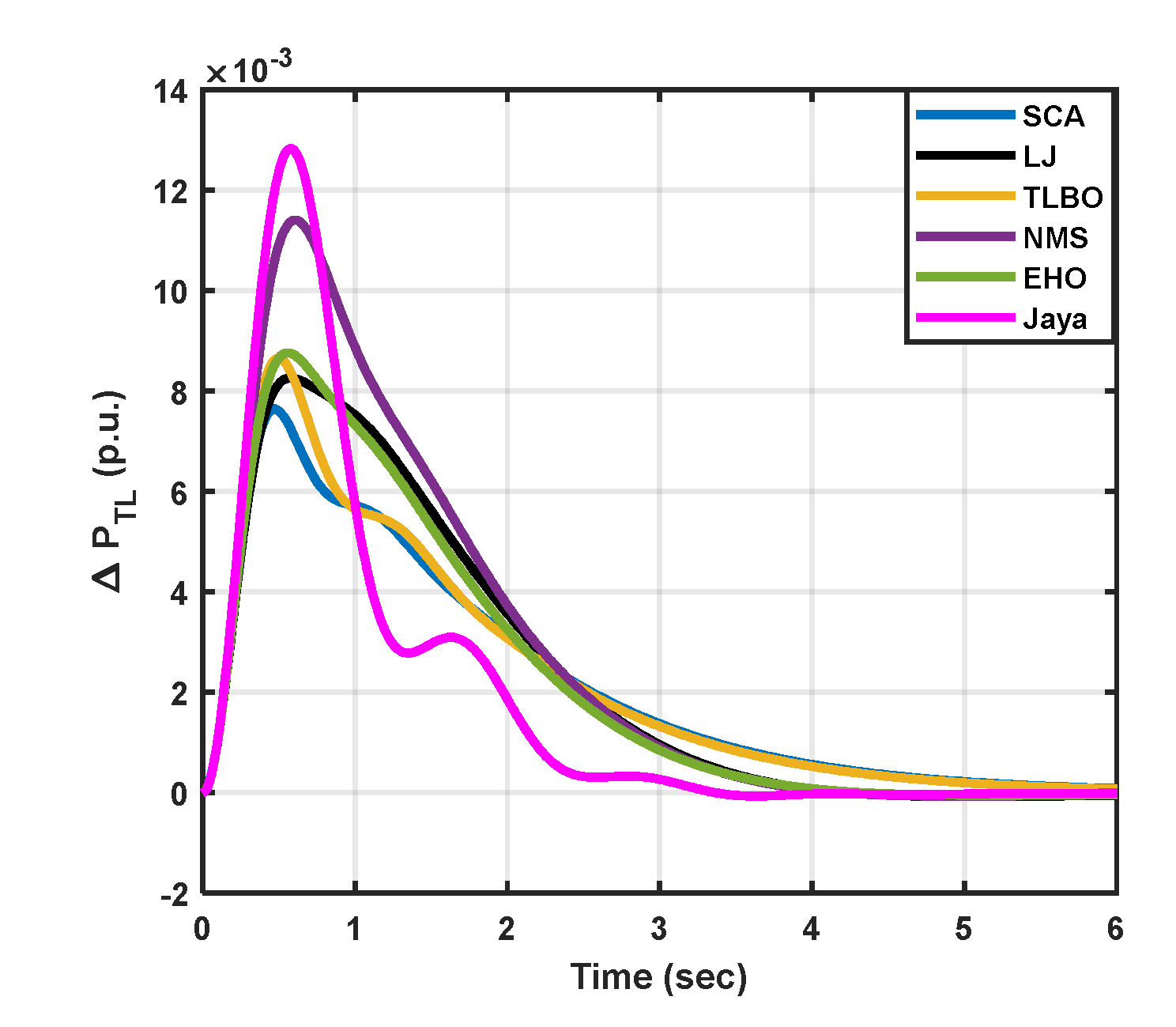
Figure 18.
Case VI: Frequency fluctuations for area-2.
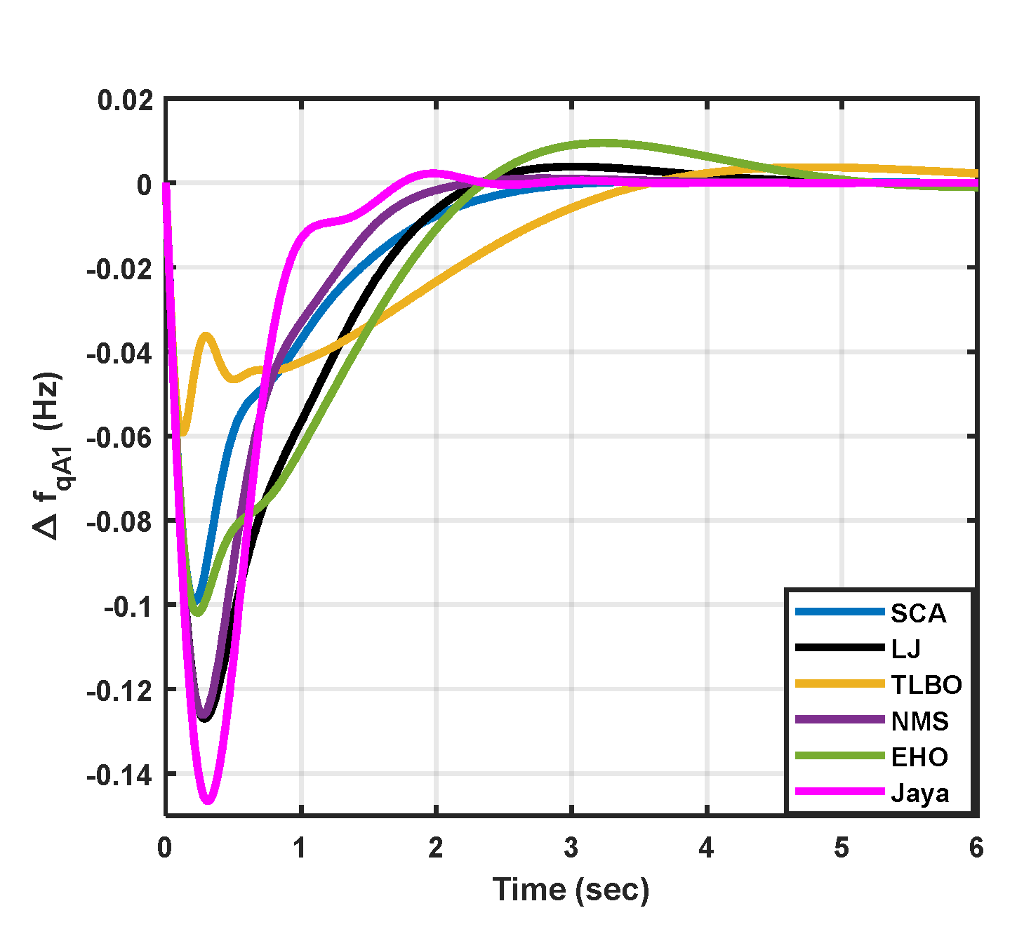
Figure 19.
Case VI: Frequency fluctuations for area-2.
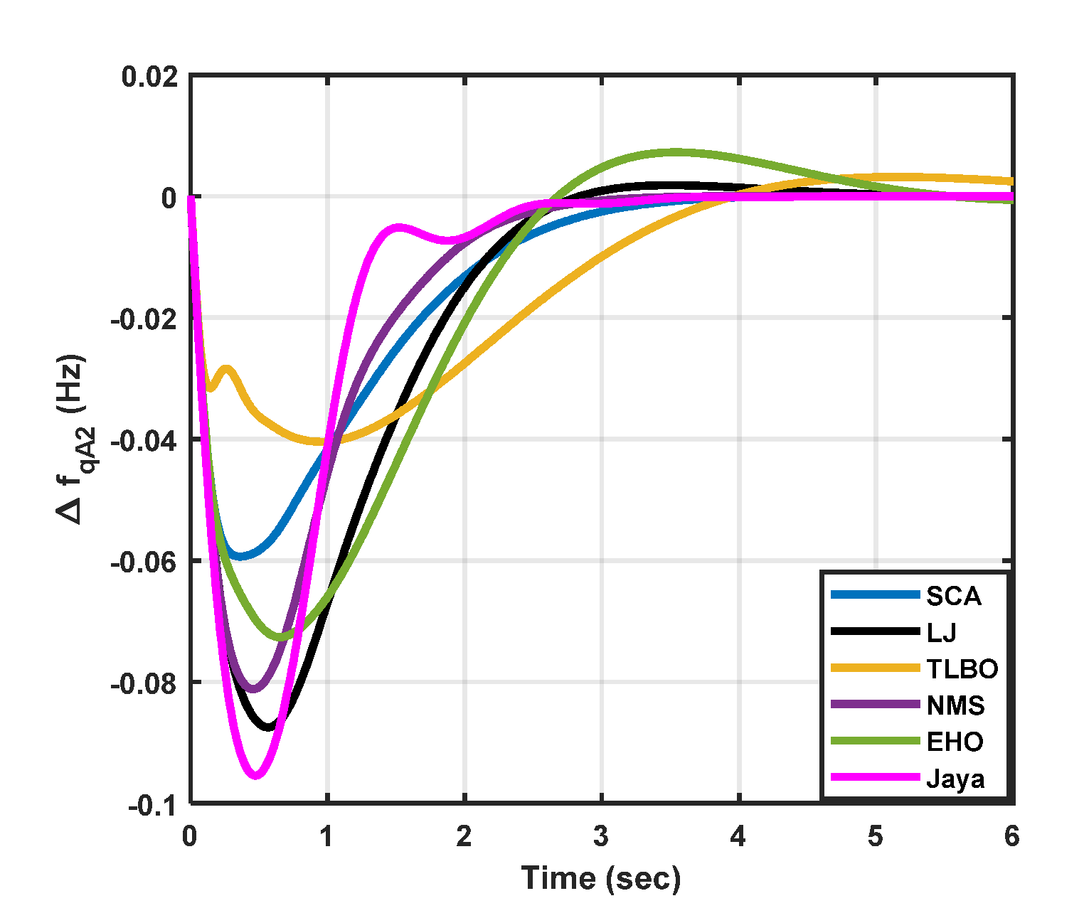
Figure 20.
Case VI: Tie-line power fluctuation.
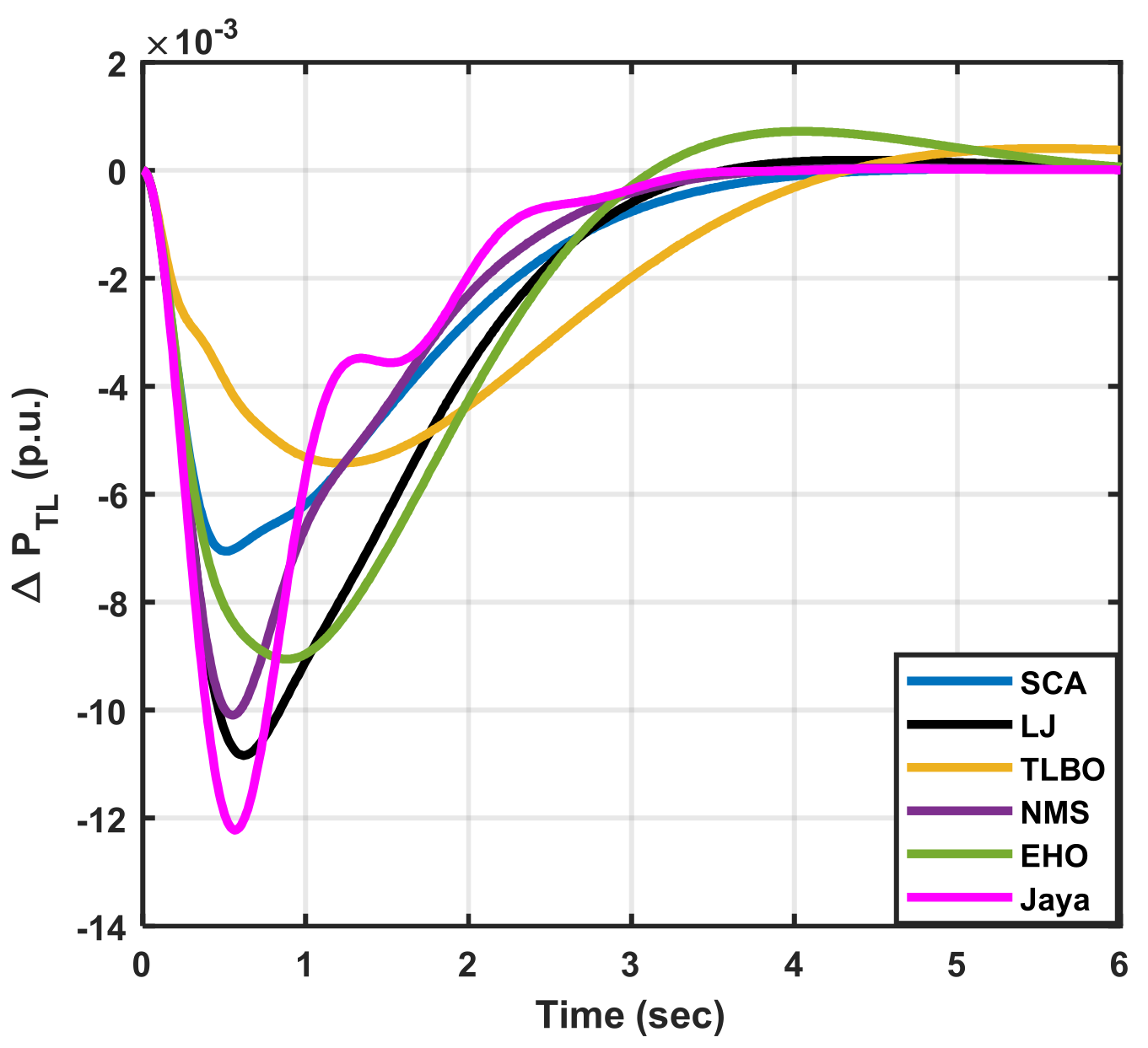

Table 1.
Decision matrix.
| Attributes | |||
|---|---|---|---|
| Alternative |
() 40% |
() 40% |
() 20% |
| Highest | Highest | Moderately high | |
| Moderate | Moderate | Extremely high | |
| High | High | Moderate | |
Table 2.
Decision matrix with performance indices.
| Attributes | |||
|---|---|---|---|
| Alternative |
() 40% |
() 40% |
() 20% |
| 100 | 100 | 70 | |
| 50 | 50 | 90 | |
| 60 | 60 | 50 | |
Table 3.
Decision matrix with scores.
| Attributes | |||
|---|---|---|---|
| Alternative |
() 0.4 |
() 0.4 |
() 0.2 |
| 1 | 1 | 0.66 | |
| 0.44 | 0.44 | 0.89 | |
| 0.55 | 0.55 | 0.44 | |
Table 4.
Decision matrix with cumulative scores.
| Attributes | ||||
|---|---|---|---|---|
| Alternative |
() 0.4 |
() 0.4 |
() 0.2 |
Cumulative scores |
| 0.4 | 0.4 | 0.132 | 0.93 | |
| 0.176 | 0.176 | 0.178 | 0.53 | |
| 0.22 | 0.22 | 0.088 | 0.528 | |
Table 5.
Decision matrix with normalized cumulative scores.
| Attributes | |||||
|---|---|---|---|---|---|
| Alternative |
() 0.4 |
() 0.4 |
() 0.2 |
Cumulative scores |
Normalized cumulative scores |
| 0.4 | 0.4 | 0.132 | 0.93 | 0.467 | |
| 0.176 | 0.176 | 0.178 | 0.53 | 0.266 | |
| 0.22 | 0.22 | 0.088 | 0.528 | 0.265 | |
Table 6.
Case studies.
| Step load variations | ||
|---|---|---|
| Case studies | Area 1 | Area 2 |
| I | 0.07 | 0 |
| II | 0 | 0.07 |
| III | 0.07 | 0.07 |
| IV | 0.07 | -0.07 |
| V | 0.07 | 0.14 |
| VI | 0.14 | 0.07 |
Table 7.
Results for case study I.
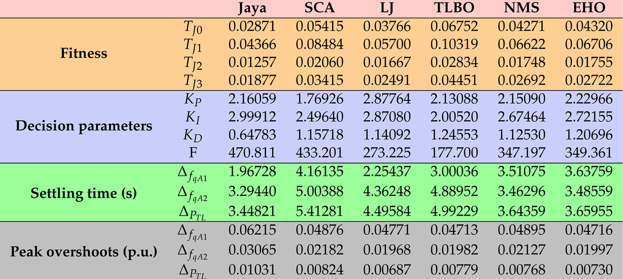 |
Table 8.
Results for case study II
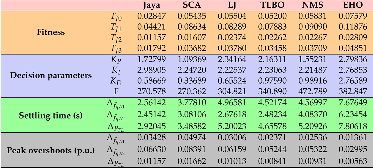 |
Table 9.
Results for case study III.
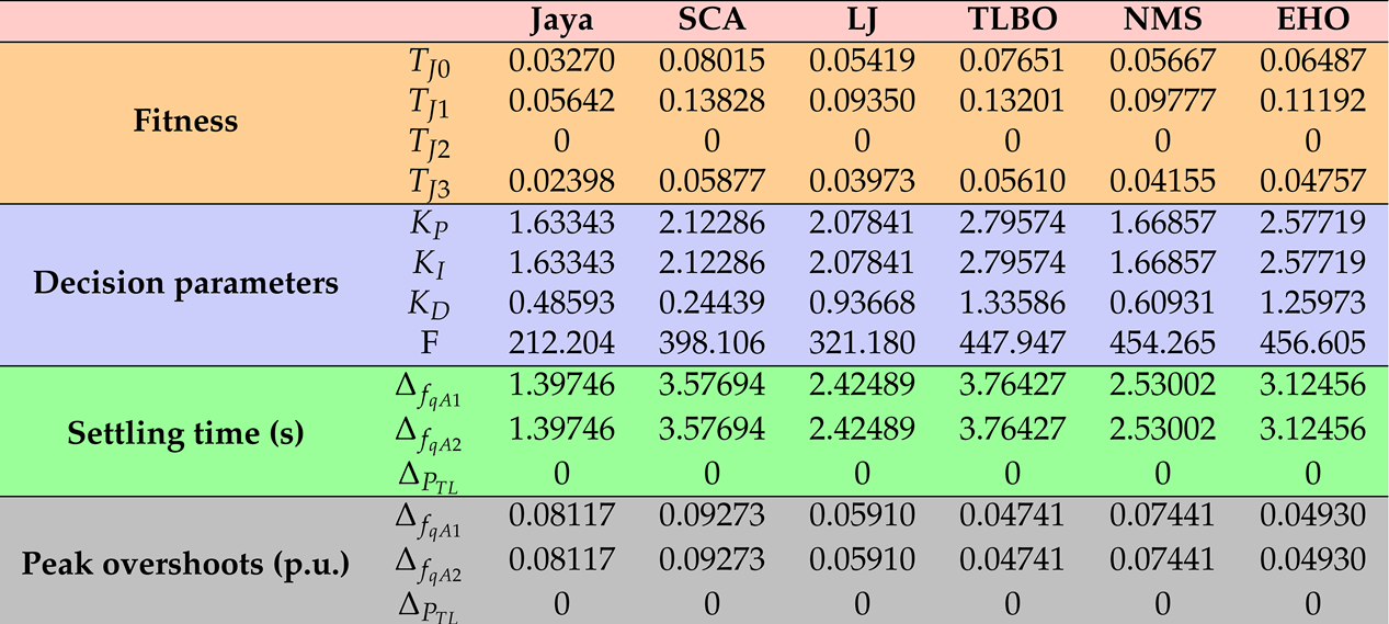 |
Table 10.
Results for case study IV.
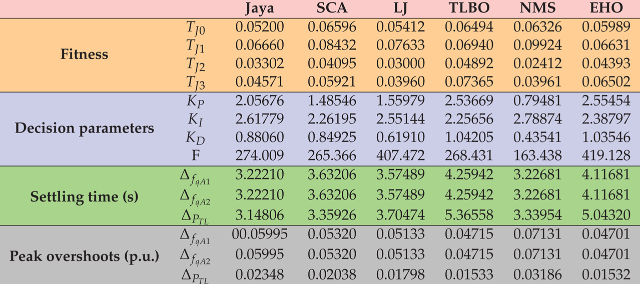 |
Table 11.
Results for case study V.
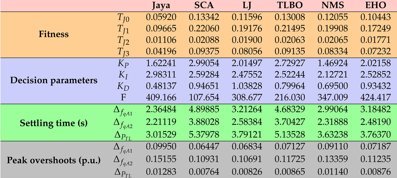 |
Table 12.
Results for case study VI.
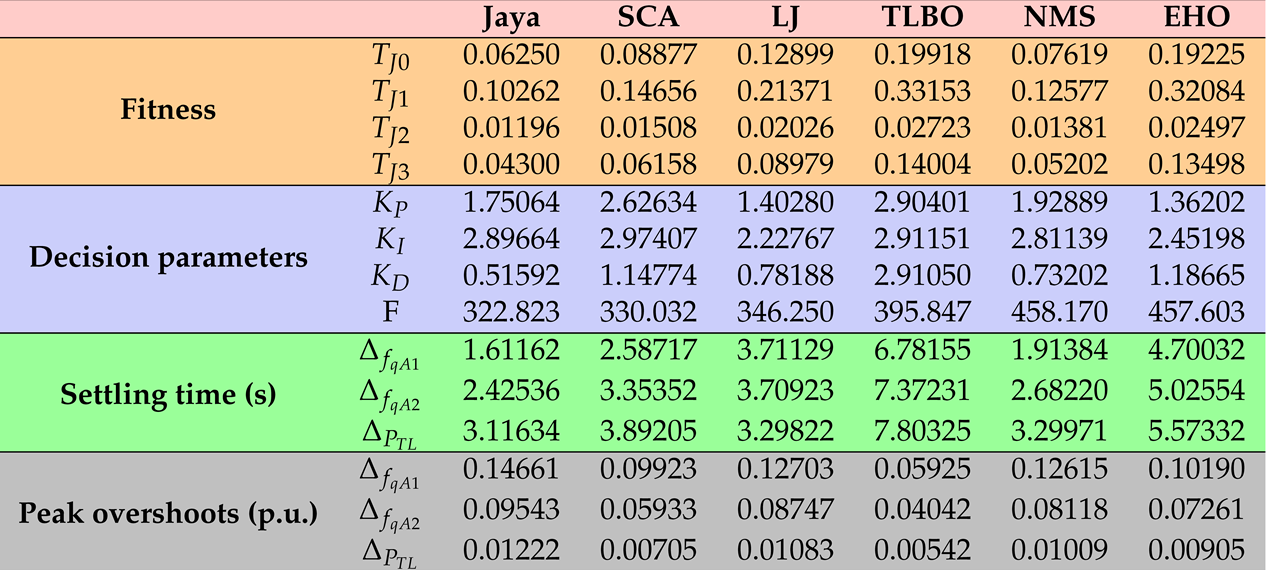 |
Table 13.
Statistical analysis.
| Cases | Statistical measures | Jaya | SCA | LJ | TLBO | NMS | EHO |
|---|---|---|---|---|---|---|---|
| I | Mean | 0.02976 | 0.09934 | 0.06514 | 0.08390 | 0.04687 | 0.05063 |
| Min | 0.02871 | 0.05415 | 0.03766 | 0.06752 | 0.04271 | 0.04320 | |
| Max | 0.03343 | 0.13681 | 0.09762 | 0.12246 | 0.05011 | 0.06231 | |
| Standard deviation | 0.00205 | 0.03024 | 0.02580 | 0.02375 | 0.00296 | 0.00804 | |
| II | Mean | 0.02913 | 0.09286 | 0.10004 | 0.07604 | 0.08159 | 0.07970 |
| Min | 0.02847 | 0.05435 | 0.05504 | 0.05200 | 0.05831 | 0.07579 | |
| Max | 0.02974 | 0.16590 | 0.19179 | 0.10603 | 0.10371 | 0.08434 | |
| Standard deviation | 0.00047 | 0.04909 | 0.05450 | 0.02037 | 0.01794 | 0.00359 | |
| III | Mean | 0.04533 | 0.23470 | 0.10134 | 0.11566 | 0.11939 | 0.11585 |
| Min | 0.03270 | 0.08015 | 0.05419 | 0.07651 | 0.05667 | 0.06487 | |
| Max | 0.06973 | 0.42988 | 0.14667 | 0.15864 | 0.14458 | 0.13495 | |
| Standard deviation | 0.01500 | 0.12540 | 0.03525 | 0.03032 | 0.03572 | 0.02878 | |
| IV | Mean | 0.06296 | 0.06780 | 0.08167 | 0.08457 | 0.07379 | 0.06663 |
| Min | 0.05200 | 0.06596 | 0.05412 | 0.06494 | 0.06326 | 0.05989 | |
| Max | 0.06848 | 0.07229 | 0.10889 | 0.11664 | 0.09765 | 0.07052 | |
| Standard deviation | 0.00268 | 0.00630 | 0.02395 | 0.02210 | 0.01455 | 0.00404 | |
| V | Mean | 0.06900 | 0.29577 | 0.21858 | 0.20074 | 0.13704 | 0.13045 |
| Min | 0.05920 | 0.13342 | 0.11596 | 0.13008 | 0.12055 | 0.10443 | |
| Max | 0.08900 | 0.59853 | 0.36557 | 0.35189 | 0.15336 | 0.16432 | |
| Standard deviation | 0.01222 | 0.19395 | 0.10443 | 0.08977 | 0.01526 | 0.02889 | |
| VI | Mean | 0.07210 | 0.16302 | 0.33597 | 0.21898 | 0.16838 | 0.24129 |
| Min | 0.06250 | 0.08877 | 0.12899 | 0.19918 | 0.07619 | 0.19225 | |
| Max | 0.08819 | 0.30000 | 0.66838 | 0.25634 | 0.21956 | 0.28512 | |
| Standard deviation | 0.01110 | 0.08392 | 0.22385 | 0.02429 | 0.06345 | 0.04132 |
Table 14.
Friedman rank test.
| Friedman rank test | ||||||
|---|---|---|---|---|---|---|
| Jaya | SCA | LJ | TLBO | NMS | EHO | |
| Mean rank | 1 | 4.6666 | 4.6666 | 4 | 3.5 | 3.1666 |
| Q value | Q=16 | |||||
| p value | p=0.006844 | |||||
Disclaimer/Publisher’s Note: The statements, opinions and data contained in all publications are solely those of the individual author(s) and contributor(s) and not of MDPI and/or the editor(s). MDPI and/or the editor(s) disclaim responsibility for any injury to people or property resulting from any ideas, methods, instructions or products referred to in the content. |
© 2023 by the authors. Licensee MDPI, Basel, Switzerland. This article is an open access article distributed under the terms and conditions of the Creative Commons Attribution (CC BY) license (https://creativecommons.org/licenses/by/4.0/).
Copyright: This open access article is published under a Creative Commons CC BY 4.0 license, which permit the free download, distribution, and reuse, provided that the author and preprint are cited in any reuse.


