

Submitted:
15 November 2023
Posted:
17 November 2023
You are already at the latest version
Abstract
The quadratic unconstrained binary optimization (QUBO) is a classic NP-hard problem with an enormous number of applications. Local search strategy (LSS) is one of the most fundamental algorithmic concepts that has been successfully applied to a wide range of hard combinatorial optimization problems. One LSS that has gained the attention of researchers is the r-flip (also known as r-Opt) strategy. Given a binary solution with n variables, the r-flip strategy ‘flips’ r binary variables to get a new solution if the changes improve the objective function. The main purpose of this paper is to develop several results for implementation of r-flip moves in QUBO, including a necessary and sufficient condition that when a 1-flip search reaches local optimality, the number of candidates for implementation of the r-flip moves can be reduced significantly. The results of the substantial computational experiments are reported to compare an r-flip strategy embedded algorithm and a multiple start tabu search algorithm on a set of benchmark instances and three very-large-scale QUBO instances. The r-flip strategy implemented within the algorithm makes the algorithm very efficient, very high-quality solutions within a short CPU time.
Keywords:
Combinatorial optimization
; Quadratic unconstrained binary optimization
; Local optimality
; r-flip local optimality
1. Introduction
The quadratic unconstrained binary optimization is a classic NP-hard problem with an enormous number of real has been used as a unifying approach to many combinatorial optimization problems [2,3]. Due to its practicality, as well as theoretical interest, over the years researchers have proposed many theoretical results as well as simple and sophisticated approaches as solution procedures [4,5,6,7,8,9,10,11]. However, due to the complexity and practicality of QUBO it is still necessary to provide results suitable for solving large-scale problems. In recent years, researchers have developed theoretical results to reduce algorithmic implementation difficulty of QUBO, [12,13,14,15,16,17]. Our result in this paper also helps to reduce size and difficulty of algorithmic implementation of these problems.
The quadratic unconstrained binary optimization (QUBO) can be formulated as,
In (1), is the i,j-th entry of a given n by n symmetric matrix Q. QUBO is often referred to as the model [18]. Since , and Q may be written as an upper triangular matrix by doubling each entry of the upper triangle part of the matrix and letting , then we can write (1) as (2).
Local search strategy (LSS) is one of the most fundamental algorithmic concepts that has been successfully applied to a wide range of hard combinatorial optimization problems. The basic ingredient of almost all sophisticated heuristics is some variation of LSS. One LSS that has been used by many researchers as a stand-alone or as a basic component of more sophisticated algorithms is the r-flip (also known as r-Opt) strategy [12,19,20,21,22,23]. In Figure A6, we present a comprehensive review of r-flip strategies applied to QUBO. Let N={1,2,…,n}. Given a binary solution, of , the r-flip search chooses a subset,, with , and builds a new solution, , where for all . If improves the objective function, it is called an improving move (or improving subset S). The r-flip search starts with a solution x, chooses an improving subset S, and flips all elements in S. The process continues until there is no subset S with that improves the objective function. The result is called a locally optimal solution with respect to the r-flip move (or r-Opt).
Often in strategies where variable neighborhood searches, such as fan-and-filter (F&F) [24,25], variable neighborhood search (VNS) [26,27], and multi-exchange neighborhood search (MENS)[19,20,21,22,23] are used, the value of r dynamically changes as the search progresses. Generally, there are two reasons for a dynamically changing search space strategy.
- a)
- The execution of an implementation of an r-flip local search, for larger value of r, can be computationally expensive to execute. This is because the size of the search space is of order n chosen r, and for fixed values of n, it grows quickly in r for value of . Hence, smaller values of r, especially r equal to 1 and 2, have shown considerable success.
- b)
- In practice, a r-flip local search process with a small value of r (e.g., r=1) can quickly reach local optimality. Thus, as a way to escape 1-flip local optimality, researchers have tried to dynamically change the value of r as the search progressed. This gives an opportunity to expand the search to a more diverse solution space.
A clever implementation of (a) and (b) in an algorithm can not only save computational time, since the smaller value of r is less computationally expensive, but it can also possibly reach better solutions because the larger values of r provide an opportunity to search more a diverse part of the solution space.
1.1. Previous Works
The development of closed form formulas for r-flip moves is desirable for developing heuristics for solving very-large-scale problem instances because it can reduce computational time consumed by an implementation of an algorithm. Alidaee, Kochenberger [12] introduced several theorems showing closed form r-flip formulas for general Pseudo-Boolean Optimization. Authors in [13,14] recently provided closed form formulas for evaluating r-flip rules in QUBO. In particular, Theorem 6 in [12] is specific to the problem. To explain the closed form formula for the r-flip rule in , we first introduce a few definitions. Refer to Figure A6 for an exhaustive literature of r-flip rules applied to QUBO.
Given a solution , the derivative of f(x) with respect to is defined as:
Fact 1. Given a solution vector and a solution obtained by flipping the ith element of x, we have:
It is well known that any locally optimal solution to an instance of the QUBO problem with respect to a 1-flip search satisfies,
Furthermore, after changing x to x’, the update for , j=1,…,n, can be calculated as follows:
Note that may be written as , which can simplify the implementation process. A simple 1-flip search is provided in Figure 1. Note that in line 3 we chose a sequence to implement Fact 1. Using such a strategy has experimentally proven to be very effective in several recent studies [28].
Before we present the algorithms in this study for the r-flip strategy, the notations used are given as follows:
n The number of variables
x A starting feasible solution
x* The best solution found so far by the algorithm
K The largest value of k for r-flip, kr
π(i) The i-th element of x in the order π(1)⋯π(n)
S ={i:xi is tentatively chosen to receive a new value to produce a new solution xi'} restricting consideration to |S| = r
D The set of candidates for an improving move
Tabu_ten The maximum number of iterations for which a variable can remain Tabu
Tabu(i) A vector representing Tabu status of x
Derivative of f(x) with respect to
The vector of derivatives
x(.) A vector representing the solution of x
E(.) A vector representing the value of derivative
The result of Fact 1 has been extended to the r-flip search, given below.
(Theorem 6, Alidaee, Kochenberger [12]) Let x be a given solution of QUBO and x’ obtained from x by r-flip move (for a chosen set S) where , |S|=r, the change in the value of the objective function is:
Furthermore, after changing x to x’ the update for ,j=1,…,n, can be calculated as follows:
As explained in [12], the evaluation of change in the objective function (7) can be done in , i.e., evaluating f(x’) from f(x). The update in (8) requires r calculations for each j in N\S, and r-1 calculations for each j in S, Thus, overall, update for all n variables can be performed in O(nr).
Note that for any two elements i,j=1,…,n, and i<j, we can define:
Using (9), a useful way to express Equation (7) is Equation (10).
A simple exhaustive r-flip search is provided in Figure 2. The complexity of the problem indicates that the use of a larger value of r in the r-flip local search can make the implementation of the search process more time consuming. Meanwhile, the larger value of r can provide an opportunity to search a more diverse area of search space and thus possibly reach better solutions. To overcome such conflicts, researchers often use r=1 (and occasionally r=2) as the basic components of their more complex algorithms, such as F&F, VNS, and MENS. Below, in Theorem 1 and Proposition 1, we prove that after reaching the locally optimal solution with respect to a 1-flip search, the implementation of an r-flip search can significantly be reduced. Further, related results are also provided to allow the efficient implementation of an r-flip search within an algorithm.
2. New Results on Closed-form Formulas
We first introduce some notations. For m<n, define (m, n) to be the number of combinations of m elements out of n, and let , and . Furthermore, Lemma 1 and Lemma 2, presented below, help to prove the results. Note that, Lemma 1 is direct deduction from previous results [12].
Lemma 1. Given a locally optimal solution with respect to a 1-flip search, we have:
Proof. Condition of local optimality in (5) indicates that:
Using this condition, we thus have:
Lemma 2. Let be any solution of the problem; then, we have:
Proof. For each pair of elements, , the left-hand-side can be or. Since |S|=r, the summation on the left-hand-side is at most equal to M.
Theorem 1: Let and M be as defined above and let be a locally optimal solution of with respect to a 1-flip search. A subset , with |S|=r, is an improving r-flip move if and only if we have:
Proof: Using (7), a subset of r elements is an improving r-flip move if and only if we have:
Since x is a locally optimal solution with respect to a 1-flip search, it follows from Lemma 1 that inequality (14) is equivalent to (15); that completes the proof.
Proposition 1: Let and M be as defined above and let be any locally optimal solution of the problem with respect to a 1-flip search. If a subset , with |S|=r, is an improving r-flip move, then we must have: .
Proof: Since x is a locally optimal solution with respect to a 1-flip search and S is an improving r-flip move, by Theorem 1, we have:
Using Lemma 2; we also have (16); which completes the proof.
The consequence of Theorem 1 is as follows. Given a locally optimal solution x with respect to a 1-flip search, if there is no subset of S with |S|=r that satisfies (13), then x is also locally optimal solution with respect to an r-flip search. Furthermore, if there is no subset S of any size that (13) is satisfied, then x is also locally optimal solution with respect to an r-flip search for all . Similar statements are also true regarding Proposition 1.
The result of Proposition1 is significant in the implementation of an r-flip search. It illustrates that, after having a 1-flip search implemented, if an r-flip search is next served as a locally optimal solution, only those elements with the sum of absolute value of derivatives less than M are eligible for consideration. Furthermore, when deciding about the elements of an r-flip search, we can easily check to see if any element by itself or with a combination of other elements is eligible to be a member of an improving r-flip move S. Example 1 below illustrates this situation.
Example 1. Consider an problem with n variables. Let be a given locally optimal solution with respect to a 1-flip search. Consider S={i,j,k,l} for a possible 4-flip move. In order to have S for an improving move, all 15 inequalities, given below in (17), must be satisfied. Of course, if the last inequality in (17) is satisfied, all other inequalities are also satisfied. This means each subset of the S is also an improving move. This is important in any dynamic neighborhood search strategies k-flip moves for in consideration.
Obviously, choosing the appropriate subset S to implement a move is critical. There are many ways to check for an improving subset S. Below, we explain two such strategies. In addition, a numerical example is given in the Appendix.
2.1. Strategy 1
We first define a set, D(n), of candidate for improving moves. Given a locally optimal solution x with respect to a 1-flip move, let the elements of x be ordered in ascending absolute value of derivatives, as given in (18).
Here, means the i-th element of x in the order . Let K be the largest value of k=1,2,…,n where the inequality (19) is satisfied. The set D(n) is now defined by (20).
Lemma 3. Any subset satisfies the necessary condition for an improving move.
Proof. It follows from Proposition 1.
There are some advantages to having elements of x in an ascending order, i.e., inequalities (18):
- the smaller the value of is, the more likely that is involved in an improving k-flip move for k<=r (this might be due to the fact that, the right-hand-side value M in (19) for given r is constant. Thus, smaller values of on the left-hand-side might help to satisfy the inequality easier.)
- because the elements of D(n) are in an ascending order of absolute values of derivatives, a straightforward implementable series of alternatives to be considered for improving subsets, S, may be the elements of the set given in (21). Note that there are a lot more subsets of D(n) compared to the sets in (21) that are the candidates for consideration in possible k-flip moves. Here we only gave one possible efficient implementable strategy.
It is important to note that, if Proposition 1 is used in the process of implementing an algorithm, given a locally optimal solution x with respect to a 1-flip search, after an r-flip implementation for a subset |S|=r with r>1, the locally optimal solution with respect to a 1-flip search for the new solution, x’, can be destroyed. Thus, if an r-flip search needed to be continued, a 1-flip search might be necessary on solution x’ before a new r-flip move can continue. However, there are many practical situations where this problem may be avoided for many subsets, especially when the problem is very-large-scale, i.e., the value of n is large, and/or Q is sparse. Proposition 2 is a weaker condition of Proposition 1 that can help to overcome up to some point in the aforementioned problem.
In the proof of Theorem 1 and Proposition 1, we only used a condition of optimality for a 1-flip search satisfied for the members of the subset S. We now define a condition as follows and call it ‘condition of optimality with respect to a 1-flip search for a set S’, or simply ‘condition of optimality for S’.
Given a solution x, the condition of optimality for any subset is satisfied if and only if we have:
Of course, if we have N in (22) instead of S, x is a locally optimal solution as was defined in Fact 1.
For m<n, let (m, n) be the number of combinations of m elements out of n elements, and , and . With these definitions now we state Proposition 2.
Proposition 2 (weak necessary condition): Let , |S|=r, and , and as defined above. Given any solution of , and assume the condition of optimality is satisfied for a subset S. If S is an r-flip improving move, we must have .
Proof: Similar to proof of Proposition 1.
Notice that the values of and in Proposition 2 depend on S; however, these values can be updated efficiently as the search progresses. As explained above, in situations where the problem is very-large-scale and/or Q is sparce, for many variables, the values of derivatives are ‘unaffected’ by the change of values of elements in S. This means a large set of variables still satisfies the condition of optimality, and thus the search can continue without applying a 1-flip search each time before finding a new set S for r-flip implementation.
2.2. Strategy 2
Another efficient and easily implementable strategy is when instead of (19), we only use an individual element to create a set of candidates for applying an r-flip search, set D(1) as defined below. Corollary 1 is a special case of Proposition 1 that suffices such a strategy.
Corollary 1: Let and M be as defined before, given a solution of , if the 1-flip local search cannot further improve the value of f(x), and with where an r-flip move of elements of S improves f(x), then we must have .
To gain insight into the use of Corollary 1, we did some experimentation to find the size of the set D(1) for different sizes of instances. The steps of the experiment to find the size of D(1) are given below. Problems considered are taken from literature [27], and used by many researchers. We only used the larger-scale problems with 2500 to 6000 variables, a total of 38 instances.
Find_D(): Procedure for finding the size of the set D(1):
- Step 2. Find the number of elements in the set D(1) for x.
- Step 3. Repeat Step 1 and 2, 200 times for each problem, and find the average number of elements in the set D(1) for the same size problem, density, and r value.
The results of the experiment are shown in Table 1. From Table 1, in general we can say that as the density of matrix Q increases, the size of D(1) decreases for all problem sizes and values of r. This is, of course, due to the fact that the larger density of Q makes the derivative of each element in an x more related to other elements. As the size of a problem increases, the size of D(1) also increases.
An interesting observation in our experiment was that, in most cases, the size of D(1) for better locally optimal solutions were smaller than those with the worse locally optimal solutions. This indicates that as the search reaches closer to the globally optimal solutions, the time for an r-flip search decreases when we take advantage of Corollary 1.
2.3. Implementation Details
We first implement two strategies in Section 2.1 and Section 2.2 via Algorithm 3 for Strategy 1 (see Figure 3), and Algorithm 4 for Strategy 2 (see Figure 4), then propose Algorithm 5 for Strategy 2 embedded with a simple tabu search algorithm for the improvement in Figure 5.
In the Destruction() procedure, there are three steps:
- step 3a. Find the variable that is not on the tabu list and lead to the small change to the solution when the variable is flipped.
- step 3b. Change its value, place it on the tabu list to update the tabu list, update E(x).
- step 3c. Test if there is any variable that is not on the tabu list and can improve the solution. If not, go to Step 3a.
In the Construction() procedure, there are four steps:
- step 4a. Test all the variables that are not on the tabu list. If a solution better than the current best solution is found, change its value, place it on the tabu list, update E(x) , update the tabu list, and go to Step 1.
- step 4b. Find the index i corresponding to the greatest value of E(xi), change its value of xi, place it on the tabu list to update the tabu list, update E(x).
- step 4c. If this is the fifteenth iteration in the Construction() procedure, go to Step 1.
- step 4d. Test if there is any variable that is not on the tabu list and can improve the solution. If not, go to Step 3a. If yes, go to Step 4a.
The randChange() procedure is invoked occasionally and randomly to select an x for the Destruction() using a random number generator. There is less than a 2% probability of invoking after the Construction() procedure. To get the 2% probability, a random number generator is used to create an integer between 1 to 1000. If the value of integer is smaller than 20, the randChange() is invoked. The variable chosen in the randChange() will lead to the change of E(x) for Destruction().
Any local search algorithm, e.g., Algorithm 3 or 4, can be used in Step 1 of this simple tabu search heuristic. However, a limited preliminary implementation of Algorithm 3 and 4 within the Algorithm 5 suggested that due to its simplicity of implementation and computational saving time, the Algorithm 4 with slight modification was quite effective, thus we used it in Step 1 of the Algorithm 5. The slight modification was as follows. If the solution found by a 1-flip is worse than the current best-found solution, quit the local search and go to Step 2.
In order to determine whether the hybrid r-flip/1-flip local search algorithms with two strategies (Algorithms 3 and 4) do better than the hybrid r-flip/1-flip local search embedded with a simple tabu search implementation, we compared Algorithms 3 and 4 to Algorithm 5.
The goal of the new strategies is to reach local optimality on large scale instances with less computing time. We report the comparison of three algorithms of a 2-flip on very-large-scale QUBO instances in the next section.
3. Computational results
In this study, we perform substantial computational experiments to evaluate the proposed strategies for problem size, density, and r value. We compare the performance of Algorithms 3, 4, and 5 for r=2 on very-large-scale QUBO instances. We also compare the best algorithm among Algorithms 3, 4, and 5 to one of the best algorithms for , i.e., Palubeckis’s multiple start tabu search. We code the algorithms in C++ programming language.
In [29], there are five multiple start tabu search algorithms, and MST2 algorithm had the best results reported by the author. We choose MST2 algorithm with the default values for the parameters recommended by the author [29]. In MST2 algorithm, the number of iterations as the stopping criteria for the first tabu search start subroutine is 25000 * size of problem, then MST2 algorithm reduces the number of iterations to 10000*size of problem as the stopping criteria for the subsequent tabu search starts. Within the tabu search subroutine, if an improved solution is found, then MST2 algorithm invokes a local search immediately. The CPU time limit in MST2 algorithm is checked at the end of the tabu search start subroutine. Thus, the computing time might exceed the CPU time limit for large instances when we choose short CPU time limits.
All algorithms in this study are compiled by GNU C++ compiler v4.8.5 and run on a single core of Intel Xeon Quad-core E5420 Harpertown processors, which have a 2.5 GHz CPU with 8 GB memory. All computing jobs were submitted through the Open PBS Job Management System to ensure both methods using the same CPU for memory usage and CPU time limits on the same instance.
Preliminary results indicated that Algorithms 3, 4, and 5 perform well on instances with the size less than 3,000 and low density. All algorithms found the best-known solution with the CPU time limit of 10 seconds. Thus, we only compare the results of large instances with high density and size from 3,000 to 8,000 by MST2 algorithm and the best algorithm among Algorithms 3, 4, and 5. These benchmark instances with the size from 3,000 to 8,000 have been reported by other researchers [6,30]. In addition, we generate some very-large-scale QUBO instances with high density and size of 30,000 using the same parameters from the benchmark instances. We use a CPU time limit of 600 seconds and r=2 for Algorithms 3, 4, and 5 on the very-large-scale instances in Table 2. We adopted the following notation for computational results:
OFV The value of the objective function for the best solution found by each algorithm.
BFS Best found solution among algorithms within the CPU time limit.
TB[s] Time to reach the best solution in seconds of each algorithm.
AT[s] Average computing time out of 10 runs to reach OFV.
DT %Deviation of computing time out of 10 runs to reach OFV.
Table 2 shows the results of comparison for Algorithms 3, 4, and 5 on very-large-scale instances out of 10 runs. Algorithm 5 produces a better solution than Algorithms 3 and 4 with r=2; thus, we use Algorithm 5 with r=1 and r=2 to compare to MST2 algorithm. We impose a CPU time limit of 60 seconds and 600 seconds per run with 10 runs per instance on Algorithm 5 and MST2 algorithm. We choose tabu tenure value of 100 for 1-flip and 2-flip. The instance data and solutions files are available on this data repository1.
In our implementation, we choose the CPU time limit as the stopping criteria and check the CPU time limit before invoking the tabu search in Algorithm 5. Because MST2 algorithm and Algorithm 5 are not single point-based search methods, the choice of the CPU time limit as the stopping criteria seems to be a fair performance comparison method between algorithms.
Table 3 describes the size and density of each instance and the number of times out of 10 runs to reach the OFV as well as solution deviation within the CPU time limit for MST2 algorithm and Algorithm 5 with r=1 and r=2. MST2 algorithm produces a stable performance and reaches the same OFV frequently out of 10 runs. Algorithm 5 starts from a random initial solution and can search a more diverse solution space in a short CPU time limit. When the CPU time limit is changed to 600 seconds, MST2 algorithm and Algorithm 5 produce a better solution quality in terms of relative standard deviation[31]. The relative standard deviation (RSD) in Table 3 inside the parenthesis is measured by: , and , where f(x) is the OFV of each run and is the mean value of OFV out of n=10 runs. For some instances, the relative standard deviation (RSD) is less than 5.0E-4 even though not all runs found the same OFV. We use 0.000 as the value of RSD when the value is rounded up to three decimal points.
Table 4 reports the computational results of a CPU time limit of 60 seconds, and Table 5 reports the computational results of a CPU time limit of 600 seconds. In Table 4, MST2 algorithm matches 5 out of 27 best solutions within the CPU time limit. The 1-flip strategy in Algorithm 5 matches 26 out of 27 best solutions while the 2-flip strategy in Algorithm 5 matches 18 out of 27 best solutions. For MST2 algorithm, the computing time to find the initial solution exceeded the CPU time limit of 60 seconds for two large instances.
When the CPU time limit is increased to 600 seconds, MST2 algorithm matches 10 out of 27 best solutions. The 1-flip strategy matches 25 out of 27 best solutions, and the 2-flip strategy matches 23 out of 27 best solutions. The 1-flip and 2-flip strategies in Algorithm 5 perform well on the high-density large instances. There is no clear pattern that the 2-flip strategy uses more time than a 1-flip strategy on finding the same OFV. The 1-flip and 2-flip strategies in Algorithm 5 choose the initial solution randomly and independently. The 1-flip strategy has a better performance when the CPU time limits are 60 and 600 seconds.
Table 6 and Table 7 present the time deviation of each algorithm on reaching the OFV for each instance. MST2 algorithm has less variation in computing time when it finds the same OFV while the r-flip strategy in Algorithm 5 has a wider range of computing time. If the algorithm only finds the OFV once out of 10 runs, the time deviation will be zero.
The r-flip strategy can be embedded in other local search heuristics as an improvement procedure. The clever implementation of the r-flip strategy can reduce the computing time as well as improve the solution quality. We reported the time and solutions out of 10 runs for each instance. The time deviation and solution deviation of 10 runs with the short CPU time limits are computed due to the computing resources available to this study.
4. Conclusion
In this study, we explored the Quadratic Unconstrained Binary Optimization (QUBO) problem and introduced significant findings. We established a necessary and sufficient condition for the local optimality of an r-flip search after a 1-flip search has already achieved local optimality. Our computational experiments demonstrated a substantial reduction in candidate options for r-flip implementation. The new r-flip strategy efficiently solved extremely large QUBO instances within 600 seconds, outperforming MST2 in terms of time taken to reach the best-known solutions on benchmark instances. These results are particularly promising for implementing variable neighborhood strategies on extensive problems or sparse matrices.
Author Contributions
Conceptualization, B. Alidaee and H. Wang; methodology, B. Alidaee; validation, B. Alidaee, H. Wang and L. Sua; formal analysis, H. Wang; investigation, H. Wang; data curation, H. Wang; writing—original draft preparation, B. Alidaee; writing—review and editing, H. Wang and L. Sua; visualization, B. Alidaee; All authors have read and agreed to the published version of the manuscript.
Funding
This research received no external funding.
Data Availability Statement
The instance data and solutions files are available at: https://doi.org/10.18738/T8/WDFBR5.
Conflicts of Interest
The authors declare no conflict of interest.
Appendix A. Numerical example for Theorem 1 and Proposition 1
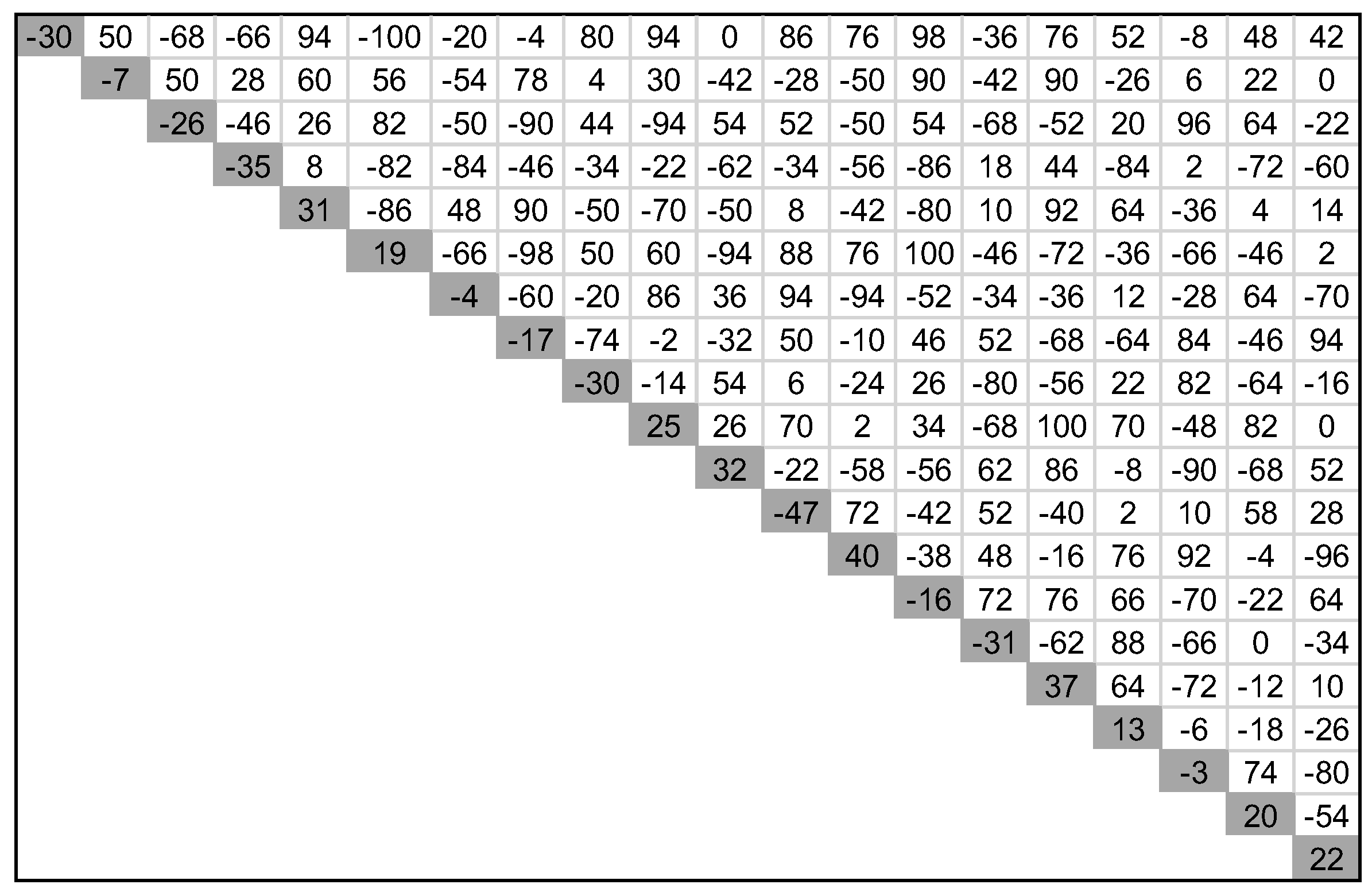
Numerical Example. Consider the problem with Q matrix given below, Figure A1. A locally optimal solution x with f(x)=1528 and the vector of derivatives, E(x) is shown in Figure A2. For r=2, M=100, every two elements that satisfy Proposition 1 is shown in Figure A3. However, only improving two elements are those shown in red font in Figure A4. These are the two elements that satisfy Theorem 1. The new results of f(x) and E(x) on the two elements are shown in Figure A4. In this simple problem, instead of comparing 380 two element combination we only need to compare 21 combinations. Out of these 21 combinations we have 6 possible improving combinations in Figure A5.
Figure A1.
Matrix Q, for maximizing
.
Figure A2.
A locally optimal solution, x(.), and values of E(xi),i=1,…,n.

E(x1)= -30 + (50*1 - 68*0 - 66*0 + 94*1 - 100*0 - 20*1 - 4*0 + 80*0 + 94*1 + 0*0 + 86*1 + 76*1 + 98*1 - 36*0 + 76*1 + 52*1 - 8*0 + 48*1 + 42*0) = 624
E(x2)= -7 + 50*1 + (50*0 + 28*0 + 60*1 + 56*0 - 54*1 + 78*0 + 4*0 + 30*1 - 42*0 - 28*1 - 50*1 + 90*1 - 42*0 + 90*1 - 26*1 + 6*0 + 22*1 + 0*0) = 177
E(x3) = -26 + (-68*1 + 50*1) + (-46*0 + 26*1 + 82*0 - 50*1 - 90*0 + 44*0 - 94*1 + 54*0 + 52*1 -50*1 + 54*1 - 68*0 - 52*1 + 20*1 + 96*0 + 64*1 - 22*0) = -74
E(x4) = -35 + (-66*1 + 28*1 - 46*0) + (8*1 – 82* 0 - 84*1 - 46*0 - 34*0 – 22*1 - 62*0 – 34*1 – 56*1 – 86*1 + 18*0 + 44*1 – 84*1 + 2*0 – 72*1 – 60*0) = -459
… for E(x5) to E(x19)
E(x20) =22+ (42*1+0*1-22*0-60*0+14*1+2*0-70*1+94*0-16*0+0*1+52*0+28*1-96*1+64*1-34*0+10*1-26*1+80*0-54*1)= - 66
f(x1)= 1*( -30 + 50 + 94 – 20 + 94 + 86 + 76 + 98 + 76 + 52 + 48)=624
f(x2)= 1*( -7 + 60 – 54 + 30 – 28 – 50 + 90 + 90 – 26 + 22)=127
f(x3)= 0*(26 – 50 – 94 + 52 – 50 + 54 – 52 + 20 + 64)=0
… for f(x4) to f(x19)
f(x20)=0*(22)=0
f(x) = 624 + 127 + 55 + 70 + 383 + 3 + 58 + 104 + 89 – 5 + 20 = 1528
Figure A3.
Indicated elements satisfy Proposition 1. Only indicated two elements with red font can improve f(x), which satisfy Theorem 1.
Figure A3.
Indicated elements satisfy Proposition 1. Only indicated two elements with red font can improve f(x), which satisfy Theorem 1.
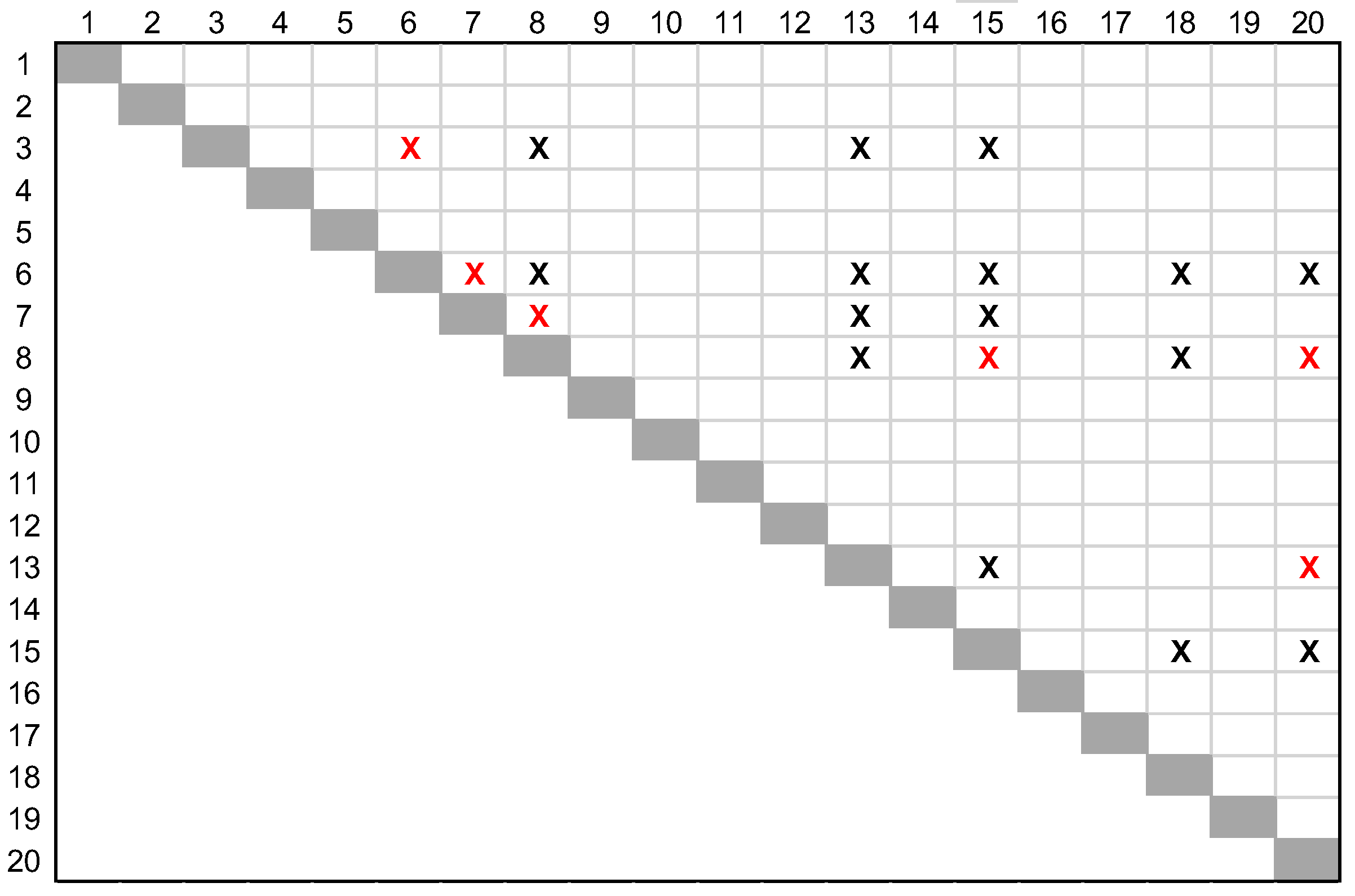
Figure A4.
An improvement using 2-flip for the locally optimal solution, x, and values of E(xi),i=1,…,n.
Figure A4.
An improvement using 2-flip for the locally optimal solution, x, and values of E(xi),i=1,…,n.

f(x1)= 1*( - 30 + 50 + 94 – 4 + 94 + 86 + 76 + 98 – 36 + 76 + 52 + 48 + 42)=646
f(x2)= 1*(-7 + 60 + 78 + 30 – 28 – 50 + 90 – 42 + 90 – 26 + 22)=217
…for f(x3) to f(x18)
f(x19)=1*(20-54)=-34
f(x20)=1*(22)=22
f(x) = 646 + 217 + 121 + 35 + 315 + 83 + 10 + 240 – 39 + 99 – 31 – 34 + 22=1684
Figure A5.
All 6 possible improving combinations for the locally optimal solution (f(x)=1528).
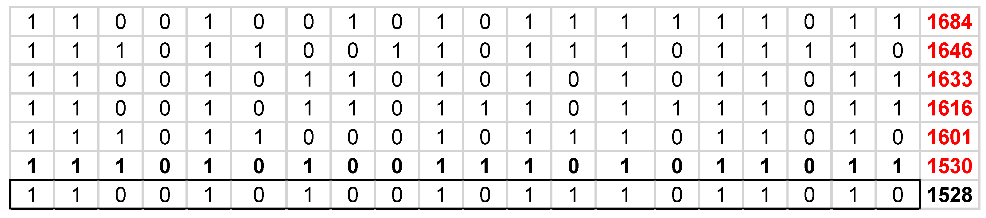

Table A1.
An exhaustive search of r-flip rules for QUBO.
| Study | r-flip rules |
| Alidaee, B., G. Kochenberger, and H. Wang, Int. J. Appl. Metaheuristic Comput., 2010. [12] | Proved several theoretical results for r-flip moves in the general psudo-boolean optimization including QUBO. |
| Anacleto, E, Meneses, C, Ravelo, S, Computers & Operations Research, 2020. [13] | Two closed-form formulas for evaluating r-flip moves was presented. Effectiveness of the moves were evaluated experimentally. |
| Anacleto, E, Meneses, C, and Liang, T, Computers & Operations Research, 2021. [14] | Considered r-flip move strategy for quadratic assignment problem that can be transferred to QUBO. Closed form formula as well as experimental evaluations considered. |
| Debevre, P, Sugimura, M, and Parizy, M, Ieee Access, 2023. [3] | Formulated the automotive paint shop problem as QUBO then 1 and several flips moves provided for solution. |
| Glover, F, and Hao, J-K, Int. J. Metaheuristics, 2010. [7] | Efficiently evaluating of 2-flip moves for QUBO was presented. |
| Glover, F, and Hao, J-K, Annals of Operations Research, 2016. [8] | A class of approaches called f-flip strategies that include fractional value for f is provided for QUBO. |
| Katayama, K, and Naihisa, H, in: W. Hart, N. Krasnogor, J.E. Smith (Eds.), Recent Advances in Memetic Algorithms, Springer, Berlin, 2004. [32] | k-flip move in the context of a memetic algorithm was presented. |
| Liang, R.N, Anacleto, E.A.J, and Meneses, C.N. Computers & Operations Research, 2023. [33] | A closed-form formulae for psuedo boolean optimization as well as data structure for efficient implementation of 1-flip rule presented. |
| Lozano, M, Molina, D, and Garcia-Martinez, C, European Journal of Operational Research, 2011. [11] | Considered maximum diversity problem which is a QUBO with added number of variables that must be equal to an integer m. A 2-flip strategy with computational experiment was presented. |
| Lu, Z., Glover, F., & Hao, J.K. in M. Caserta and S. Voss (Eds.): Metaheuristics International Conference 2011 Post-Conference Book, Chapter 4. [34] | Several combinations of neighborhood structures based on 1 and 2-flip strategy for QUBO within the context of tabu search present. |
| Merz, P, and Freisleben, B, Journal of Heuristics, 2002. [35] | Provided 1 and several flips strategy for QUBO and provided computational experiment. |
| Rosenberg, G., Vazifeh, M, Woods, B, and Haber, E, Computational Optimization and Applications, 2016. [30] | A k-flip strategy in the context of quantum annealer. |
References
- Szeider, S. The parameterized complexity of k-flip local search for SAT and MAX SAT. Discrete Optimization 2011, 8, 139–145. [Google Scholar] [CrossRef]
- Boros, E.; Hammer, P.L.; Minoux, M.; Rader, D.J. Optimal cell flipping to minimize channel density in VLSI design and pseudo-Boolean optimization. Discret. Appl. Math. 1999, 90, 69–88. [Google Scholar] [CrossRef]
- Debevere, P.; Sugimura, M.; Parizy, M. Quadratic Unconstrained Binary Optimization for the Automotive Paint Shop Problem. IEEE Access 2023, 11, 97769–97777. [Google Scholar] [CrossRef]
- Glover, F.; Kochenberger, G.; Du, Y. Quantum Bridge Analytics I: a tutorial on formulating and using QUBO models. 4OR 2019, 17, 335–371. [Google Scholar] [CrossRef]
- Glover, F.; Kochenberger, G.A.; Alidaee, B. Adaptive Memory Tabu Search for Binary Quadratic Programs. Manag. Sci. 1998, 44, 336–345. [Google Scholar] [CrossRef]
- Glover, F.; Lü, Z.; Hao, J.-K. Diversification-driven tabu search for unconstrained binary quadratic problems. 4OR 2010, 8, 239–253. [Google Scholar] [CrossRef]
- Glover, F.; Hao, J.K. Fast two-flip move evaluations for binary unconstrained quadratic optimisation problems. Int. J. Metaheuristics 2010, 1, 100. [Google Scholar] [CrossRef]
- Glover, F.; Hao, J.-K. f-Flip strategies for unconstrained binary quadratic programming. Ann. Oper. Res. 2015, 238, 651–657. [Google Scholar] [CrossRef]
- Kochenberger, G.; Hao, J.-K.; Glover, F.; Lewis, M.; Lü, Z.; Wang, H.; Wang, Y. The unconstrained binary quadratic programming problem: a survey. J. Comb. Optim. 2014, 28, 58–81. [Google Scholar] [CrossRef]
- Kochenberger, G.A.; Glover, F.; Wang, H. Binary Unconstrained Quadratic Optimization Problem. In Handbook of Combinatorial Optimization; Pardalos, P.M., Du, D.-Z., Graham, R.L., Eds.; Springer: New York, NY, USA, 2013; pp. 533–557. [Google Scholar]
- Lozano, M.; Molina, D.; Garcı´a-Martı´nez, C. Iterated greedy for the maximum diversity problem. Eur. J. Oper. Res. 2011, 214, 31–38. [Google Scholar] [CrossRef]
- Alidaee, B.; Kochenberger, G.; Wang, H. Theorems Supporting r-flip Search for Pseudo-Boolean Optimization. Int. J. Appl. Metaheuristic Comput. 2010, 1, 93–109. [Google Scholar] [CrossRef]
- Anacleto, E.A.; Meneses, C.N.; Ravelo, S.V. Closed-form formulas for evaluating r-flip moves to the unconstrained binary quadratic programming problem. Comput. Oper. Res. 2019, 113, 104774. [Google Scholar] [CrossRef]
- Anacleto, E.; Meneses, C.; Liang, T. Fast r-flip move evaluations via closed-form formulae for Boolean quadraticprogramming problems with generalized upper bound constraints. Computers & Operations Research 2021, 132, 105297. [Google Scholar]
- Glover, F.; Lewis, M.; Kochenberger, G. Logical and inequality implications for reducing the size and difficulty of quadratic unconstrained binary optimization problems. Eur. J. Oper. Res. 2018, 265, 829–842. [Google Scholar] [CrossRef]
- Lewis, M.; Glover, F. Quadratic unconstrained binary optimization problem preprocessing: Theory and empirical analysis. Networks 2017, 70, 79–97. [Google Scholar] [CrossRef]
- Vredeveld, T.; Lenstra, J.K. On local search for the generalized graph coloring problem. Oper. Res. Lett. 2003, 31, 28–34. [Google Scholar] [CrossRef]
- Kochenberger, G.; Glover, F. Introduction to special xQx issue. J. Heuristics 2013, 19, 525–528. [Google Scholar] [CrossRef]
- Ahuja, R.K.; Ergun, *!!! REPLACE !!!*; Orlin, J.B.; Punnen, A.P. A survey of very large-scale neighborhood search techniques. Discret. Appl. Math. 2002, 123, 75–102. [Google Scholar] [CrossRef]
- Ahuja, R.K.; Orlin, J.B.; Pallottino, S.; Scaparra, M.P.; Scutellà, M.G. A Multi-Exchange Heuristic for the Single-Source Capacitated Facility Location Problem. Manag. Sci. 2004, 50, 749–760. [Google Scholar] [CrossRef]
- Yagiura, M.; Ibaraki, T. Analyses on the 2 and 3-Flip Neighborhoods for the MAX SAT. J. Comb. Optim. 1999, 3, 95–114. [Google Scholar] [CrossRef]
- Yagiura, M.; Ibaraki, T. Efficient 2 and 3-Flip Neighborhood Search Algorithms for the MAX SAT: Experimental Evaluation. J. Heuristics 2001, 7, 423–442. [Google Scholar] [CrossRef]
- Yagiura, M.; Kishida, M.; Ibaraki, T. A 3-flip neighborhood local search for the set covering problem. Eur. J. Oper. Res. 2006, 172, 472–499. [Google Scholar] [CrossRef]
- Alidaee, B. Fan-and-Filter Neighborhood Strategy for 3-SAT Optimization, Hearin Center for Enterprise Science, T.U.o. Mississippi, Editor. 2004, The University of Mississippi: Hearin Center for Enterprise Science.
- Glover, F. A template for scatter search and path relinking; Springer: Berlin/Heidelberg, Germany, 1998. [Google Scholar]
- Ivanov, S.V.; Kibzun, A.I.; Mladenović, N.; Urošević, D. Variable neighborhood search for stochastic linear programming problem with quantile criterion. J. Glob. Optim. 2019, 74, 549–564. [Google Scholar] [CrossRef]
- Mladenović, N.; Hansen, P. Variable neighborhood search. Computers & Operations Research 1997, 24, 1097–1100. [Google Scholar]
- Alidaee, B.; Sloan, H.; Wang, H. Simple and fast novel diversification approach for the UBQP based on sequential improvement local search. Comput. Ind. Eng. 2017, 111, 164–175. [Google Scholar] [CrossRef]
- Palubeckis, G. Multistart Tabu Search Strategies for the Unconstrained Binary Quadratic Optimization Problem. Ann. Oper. Res. 2004, 131, 259–282. [Google Scholar] [CrossRef]
- Rosenberg, G.; Vazifeh, M.; Woods, B.; Haber, E. Building an iterative heuristic solver for a quantum annealer. Comput. Optim. Appl. 2016, 65, 845–869. [Google Scholar] [CrossRef]
- Glen, S. Relative Standard Deviation: Definition & Formula. 2014. Available online: https://www.statisticshowto.com/relative-standard-deviation/.
- Katayama, K, and Naihisa, H, An evolutionary approach for the maximum diversity problem, in: W. Hart, N. Krasnogor, J.E. Smith (Eds.), Recent Advances in Memetic Algorithms, Springer: Berlin, 2004, pp. 31–47.
- Liang, R.N.; Anacleto, E.A.; Meneses, C.N. Fast 1-flip neighborhood evaluations for large-scale pseudo-Boolean optimization using posiform representation. Comput. Oper. Res. 2023, 159, 106324. [Google Scholar] [CrossRef]
- Lu, Z., Glover, F., & Hao, J.K. Neighborhood combination for unconstrained binary quadratic problems, in M. Caserta and S. Voss (Eds.): Metaheuristics International Conference 2011 Post-Conference Book, Chapter 4, 2014; pp. 49–61.
- Merz, P.; Freisleben, B. Greedy and Local Search Heuristics for Unconstrained Binary Quadratic Programming. J. Heuristics 2002, 8, 197–213. [Google Scholar] [CrossRef]
| 1 |
Figure 1.
Pseudo-code for a 1-flip local search subroutine for maximization problems.
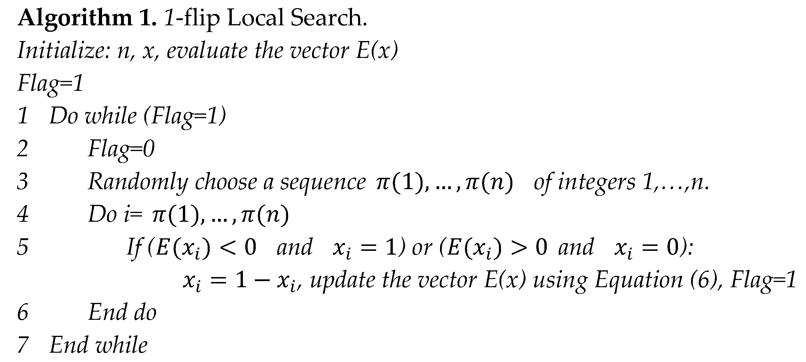
Figure 2.
Pseudo-code for an exhaustive r-flip local search subroutine for maximization problems.
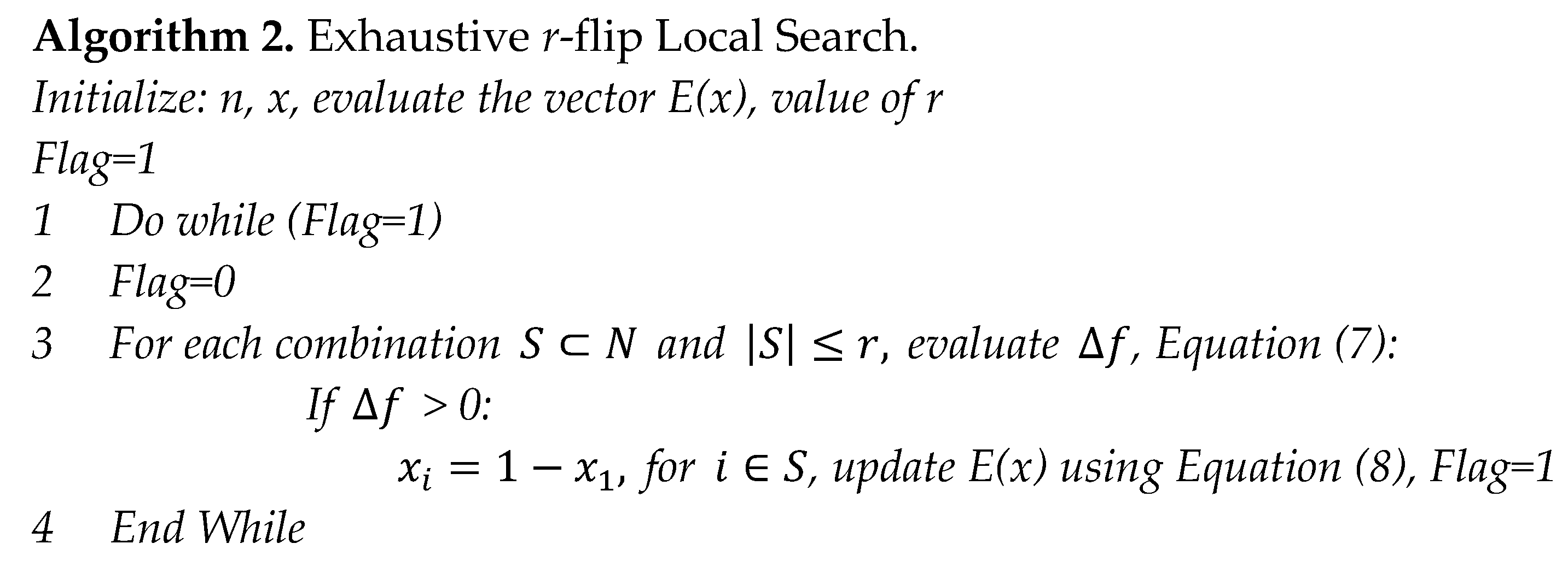
Figure 3.
Pseudo-code for hybrid r-flip/1-flip local search, Strategy 1, for maximization problems.
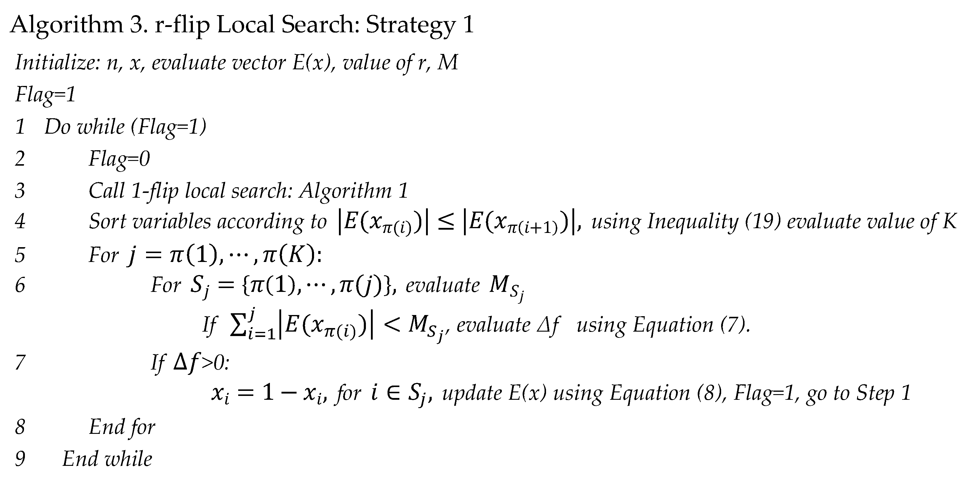
Figure 4.
Pseudo-code for hybrid r-flip/1-flip local search, Strategy 2, for maximization problems.
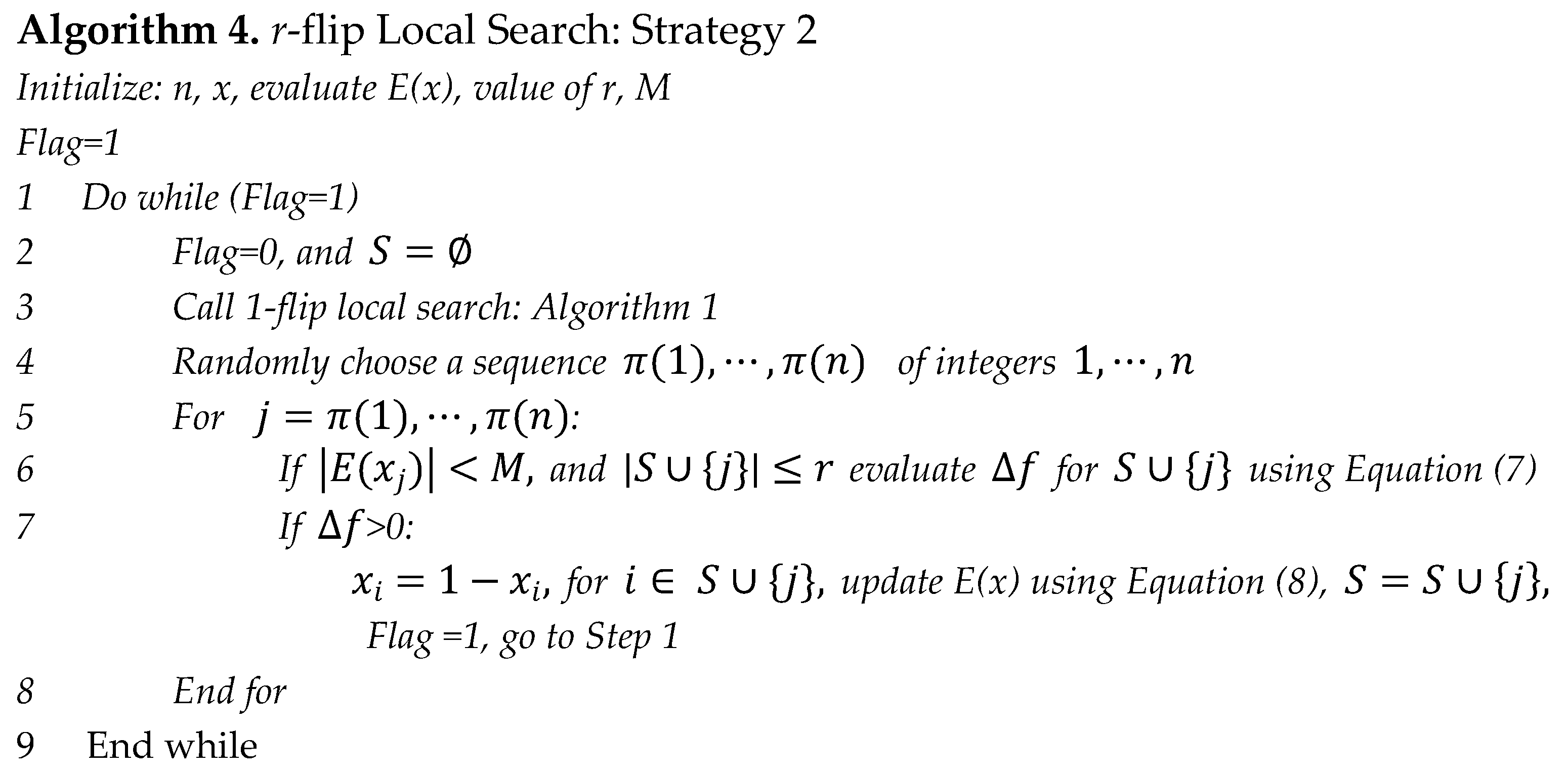
Figure 5.
Pseudo-code for hybrid r-flip/1-flip local search embedded with a simple tabu search algorithm.
Figure 5.
Pseudo-code for hybrid r-flip/1-flip local search embedded with a simple tabu search algorithm.
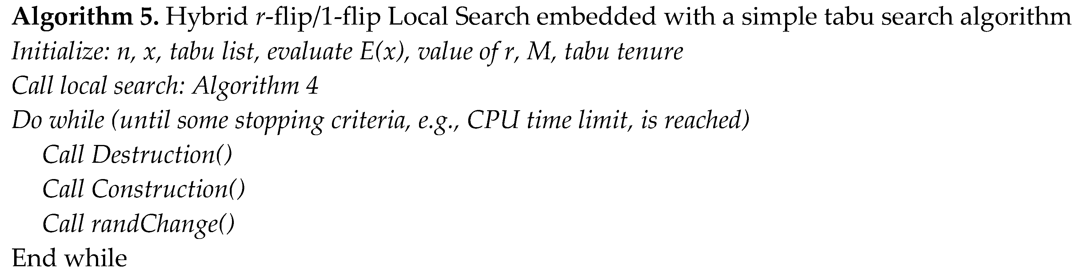
Table 1.
Size of the set D(1).
| r=2 | r=3 | r=4 | ||||||||||
| Density | ||||||||||||
| Prob. Size | 0.1 | 0.3 | 0.5 | 0.8 | 0.1 | 0.3 | 0.5 | 0.8 | 0.1 | 0.3 | 0.5 | 0.8 |
| 2500 | <100 | <40 | <30 | <20 | <400 | <200 | <100 | <100 | <1000 | <500 | <300 | <200 |
| 3000 | <100 | <40 | <30 | <20 | <400 | <200 | <100 | <100 | <1100 | <500 | <400 | <250 |
| 4000 | <100 | <30 | <30 | <20 | <500 | <200 | <100 | <100 | <1200 | <600 | <400 | <250 |
| 5000 | <100 | <30 | <30 | <20 | <500 | <200 | <100 | <100 | <1300 | <600 | <400 | <250 |
| 6000 | <100 | <30 | <30 | <20 | <500 | <200 | <100 | <100 | <1400 | <600 | <400 | <250 |
Table 2.
Results of Algorithms 3, 4 and 5 on p30000 instances with the CPU time limit of 600 seconds and r=2.
Table 2.
Results of Algorithms 3, 4 and 5 on p30000 instances with the CPU time limit of 600 seconds and r=2.
| Instance ID | size | density | Algorithm 3 | Algorithm 4 | Algorithm 5 | |||
| OFV | TB[s] | OFV | TB[s] | OFV | TB[s] | |||
| p30000_1 | 30000 | 0.5 | 127239168 | 591 | 127292467 | 591 | 127336719 | 592 |
| p30000_2 | 30000 | 0.8 | 158439036 | 572 | 158472098 | 555 | 158526518 | 571 |
| p30000_3 | 30000 | 1 | 179192241 | 584 | 179219781 | 587 | 179261723 | 590 |
Table 3.
The solution quality of MST2 algorithm and Algorithm 5 with 60- and 600-seconds time CPU limits out of 10 runs.
Table 3.
The solution quality of MST2 algorithm and Algorithm 5 with 60- and 600-seconds time CPU limits out of 10 runs.
| Instance ID | size | density | MST2 with 60s | r-flip with 60s | MST2 with 600s | r-flip with 600s | ||
| r=1 | r=2 | r=1 | r=2 | |||||
| p3000_1 | 3000 | 0.5 | 10(0) | 10(0) | 10(0) | 10(0) | 10(0) | 10(0) |
| p3000_2 | 3000 | 0.8 | 10(0) | 10(0) | 10(0) | 10(0) | 10(0) | 10(0) |
| p3000_3 | 3000 | 0.8 | 4(0.01) | 7(0.007) | 10(0) | 10(0) | 10(0) | 10(0) |
| p3000_4 | 3000 | 1 | 10(0) | 10(0) | 10(0) | 10(0) | 10(0) | 10(0) |
| p3000_5 | 3000 | 1 | 10(0) | 9(0.003) | 7(0.002) | 9(0.001) | 10(0) | 10(0) |
| p4000_1 | 4000 | 0.5 | 10(0) | 10(0) | 10(0) | 10(0) | 10(0) | 10(0) |
| p4000_2 | 4000 | 0.8 | 10(0) | 10(0) | 10(0) | 9(0.004) | 10(0) | 10(0) |
| p4000_3 | 4000 | 0.8 | 10(0) | 10(0) | 10(0) | 10(0) | 10(0) | 10(0) |
| p4000_4 | 4000 | 1 | 1(0.033) | 10(0) | 10(0) | 10(0) | 10(0) | 10(0) |
| p4000_5 | 4000 | 1 | 10(0) | 10(0) | 10(0) | 10(0) | 10(0) | 10(0) |
| p5000_1 | 5000 | 0.5 | 6(0.000) | 1(0.002) | 2(0.002) | 10(0) | 3(0.002) | 2(0.002) |
| p5000_2 | 5000 | 0.8 | 10(0) | 4(0.003) | 1(0.002) | 6(0.012) | 10(0) | 10(0) |
| p5000_3 | 5000 | 0.8 | 10(0) | 7(0.001) | 3(0.002) | 10(0) | 10(0) | 10(0) |
| p5000_4 | 5000 | 1 | 10(0) | 1(0.002) | 1(0.001) | 10(0) | 3(0.002) | 1(0.001) |
| p5000_5 | 5000 | 1 | 6(0.021) | 9(0.003) | 4(0.004) | 10(0) | 10(0) | 10(0) |
| p6000_1 | 6000 | 0.5 | 10(0) | 10(0) | 4(0.001) | 10(0) | 10(0) | 10(0) |
| p6000_2 | 6000 | 0.8 | 10(0) | 4(0.001) | 4(0.001) | 1(0.006) | 10(0) | 9(0) |
| p6000_3 | 6000 | 1 | 9(0.002) | 3(0.002) | 1(0.007) | 10(0) | 10(0) | 10(0) |
| p7000_1 | 7000 | 0.5 | 1(0.002) | 1(0.006) | 1(0.007) | 10(0) | 2(0.002) | 4(0.002) |
| p7000_2 | 7000 | 0.8 | 7(0.000) | 1(0.008) | 1(0.008) | 10(0) | 1(0.004) | 2(0.004) |
| p7000_3 | 7000 | 1 | 8(0.011) | 3(0.021) | 5(0.023) | 10(0) | 10(0) | 10(0) |
| p8000_1 | 8000 | 0.5 | 10(0) | 1(0.004) | 1(0.005) | 9(0.001) | 10(0) | 1(0.002) |
| p8000_2 | 8000 | 0.8 | 10(0) | 1(0.009) | 1(0.008) | 10(0) | 7(0.003) | 10(0) |
| p8000_3 | 8000 | 1 | 10(0) | 1(0.013) | 1(0.01) | 10(0) | 4(0.001) | 3(0.002) |
| p30000_1 | 30000 | 0.5 | 1(0.002) | 1(0.023) | 1(0.019) | 7(0.018) | 1(0.017) | 1(0.011) |
| p30000_2 | 30000 | 0.8 | 10(0) | 1(0.017) | 1(0.016) | 6(0.01) | 1(0.019) | 1(0.013) |
| p30000_3 | 30000 | 1 | 10(0) | 1(0.015) | 1(0.019) | 2(0.037) | 1(0.025) | 1(0.019) |
Table 4.
Results of MST2 algorithm and r-flip strategy in Algorithm 5 within the CPU time limit of 60 seconds.
Table 4.
Results of MST2 algorithm and r-flip strategy in Algorithm 5 within the CPU time limit of 60 seconds.
| Instance ID | BFS (60s) | MST2 (60s) | r-flip (60s) | ||||
| OFV | TB[s] | OFV(r=1) | TB[s] | OFV(r=2) | TB[s] | ||
| p3000_1 | 3931583 | 3931583 | 10 | 3931583 | 3 | 3931583 | 8 |
| p3000_2 | 5193073 | 5193073 | 25 | 5193073 | 2 | 5193073 | 2 |
| p3000_3 | 5111533 | 5111533 | 52 | 5111533 | 8 | 5111533 | 4 |
| p3000_4 | 5761822 | 5761437 | 10 | 5761822 | 2 | 5761822 | 2 |
| p3000_5 | 5675625 | 5675430 | 24 | 5675625 | 7 | 5675625 | 17 |
| p4000_1 | 6181830 | 6181830 | 40 | 6181830 | 3 | 6181830 | 4 |
| p4000_2 | 7801355 | 7797821 | 12 | 7801355 | 13 | 7801355 | 4 |
| p4000_3 | 7741685 | 7741685 | 31 | 7741685 | 5 | 7741685 | 8 |
| p4000_4 | 8711822 | 8709956 | 58 | 8711822 | 5 | 8711822 | 11 |
| p4000_5 | 8908979 | 8905340 | 27 | 8908979 | 4 | 8908979 | 13 |
| p5000_1 | 8559680 | 8556675 | 56 | 8559680 | 21 | 8559680 | 7 |
| p5000_2 | 10836019 | 10829848 | 34 | 10836019 | 59 | 10836019 | 11 |
| p5000_3 | 10489137 | 10477129 | 28 | 10489137 | 20 | 10489137 | 16 |
| p5000_4 | 12251710 | 12245282 | 52 | 12251710 | 54 | 12251520 | 42 |
| p5000_5 | 12731803 | 12725779 | 56 | 12731803 | 17 | 12731803 | 16 |
| p6000_1 | 11384976 | 11377315 | 42 | 11384976 | 12 | 11384976 | 5 |
| p6000_2 | 14333855 | 14330032 | 39 | 14333855 | 27 | 14333767 | 14 |
| p6000_3 | 16132915 | 16122333 | 51 | 16130731 | 24 | 16132915 | 48 |
| p7000_1 | 14477949 | 14467157 | 56 | 14477949 | 41 | 14476263 | 21 |
| p7000_2 | 18249948 | 18238729 | 55 | 18249948 | 47 | 18246895 | 47 |
| p7000_3 | 20446407 | 20431354 | 59 | 20446407 | 15 | 20446407 | 12 |
| p8000_1 | 17340538 | 17326259 | 47 | 17340538 | 26 | 17340538 | 35 |
| p8000_2 | 22208986 | 22180465 | 55 | 22208986 | 54 | 22208683 | 53 |
| p8000_3 | 24670258 | 24647248 | 56 | 24670258 | 43 | 24669351 | 50 |
| p30000_1 | 127252438 | 126732483 | 60 | 127252438 | 58 | 127219336 | 60 |
| p30000_2 | 158384175 | 157481366 | 69 | 158384175 | 59 | 158339497 | 60 |
| p30000_3 | 179103085 | 178093109 | 89 | 179103085 | 58 | 179029747 | 54 |
Table 5.
Results of MST2 algorithm and r-flip strategy in Algorithm 5 within the CPU time limit of 600 seconds.
Table 5.
Results of MST2 algorithm and r-flip strategy in Algorithm 5 within the CPU time limit of 600 seconds.
| Instance ID | BFS (600s) | MST2 (600s) | r-flip (600s) | ||||
| OFV | TB[s] | OFV(r=1) | TB[s] | OFV(r=2) | TB[s] | ||
| p3000_1 | 3931583 | 3931583 | 11 | 3931583 | 5 | 3931583 | 5 |
| p3000_2 | 5193073 | 5193073 | 25 | 5193073 | 1 | 5193073 | 3 |
| p3000_3 | 5111533 | 5111533 | 52 | 5111533 | 30 | 5111533 | 8 |
| p3000_4 | 5761822 | 5761822 | 269 | 5761822 | 1 | 5761822 | 2 |
| p3000_5 | 5675625 | 5675625 | 505 | 5675625 | 43 | 5675625 | 29 |
| p4000_1 | 6181830 | 6181830 | 40 | 6181830 | 4 | 6181830 | 2 |
| p4000_2 | 7801355 | 7800851 | 530 | 7801355 | 8 | 7801355 | 8 |
| p4000_3 | 7741685 | 7741685 | 30 | 7741685 | 5 | 7741685 | 2 |
| p4000_4 | 8711822 | 8711822 | 67 | 8711822 | 2 | 8711822 | 7 |
| p4000_5 | 8908979 | 8906525 | 65 | 8908979 | 4 | 8908979 | 13 |
| p5000_1 | 8559680 | 8559075 | 324 | 8559680 | 9 | 8559680 | 27 |
| p5000_2 | 10836019 | 10835437 | 541 | 10836019 | 17 | 10836019 | 21 |
| p5000_3 | 10489137 | 10488735 | 400 | 10489137 | 29 | 10489137 | 38 |
| p5000_4 | 12252318 | 12249290 | 265 | 12252318 | 127 | 12251848 | 143 |
| p5000_5 | 12731803 | 12731803 | 265 | 12731803 | 19 | 12731803 | 32 |
| p6000_1 | 11384976 | 11384976 | 406 | 11384976 | 8 | 11384976 | 39 |
| p6000_2 | 14333855 | 14333767 | 498 | 14333855 | 62 | 14333855 | 17 |
| p6000_3 | 16132915 | 16128609 | 239 | 16132915 | 60 | 16132915 | 71 |
| p7000_1 | 14478676 | 14477039 | 344 | 14478676 | 92 | 14478676 | 397 |
| p7000_2 | 18249948 | 18242205 | 587 | 18249948 | 115 | 18249844 | 43 |
| p7000_3 | 20446407 | 20431833 | 109 | 20446407 | 47 | 20446407 | 21 |
| p8000_1 | 17341350 | 17337154 | 546 | 17340538 | 45 | 17341350 | 141 |
| p8000_2 | 22208986 | 22207866 | 122 | 22208986 | 49 | 22208986 | 89 |
| p8000_3 | 24670924 | 24669797 | 402 | 24670924 | 185 | 24670924 | 386 |
| p30000_1 | 127336719 | 127323304 | 568 | 127332912 | 598 | 127336719 | 592 |
| p30000_2 | 158561564 | 158438942 | 573 | 158561564 | 580 | 158526518 | 571 |
| p30000_3 | 179329754 | 179113916 | 575 | 179329754 | 599 | 179261723 | 590 |
Table 6.
Computing the time deviation of MST2 algorithm and r-flip strategy in Algorithm 5 within the time limit of 60 seconds.
Table 6.
Computing the time deviation of MST2 algorithm and r-flip strategy in Algorithm 5 within the time limit of 60 seconds.
| Instance ID | MST2 | 1-flip | 2-flip | |||
|---|---|---|---|---|---|---|
| AT[s] | DT | AT[s] | DT | AT[s] | DT | |
| p3000_1 | 12.5 | 15.663 | 15.7 | 84.075 | 24.1 | 56.875 |
| p3000_2 | 32.5 | 20.059 | 4.9 | 45.583 | 4.8 | 68.606 |
| p3000_3 | 54.3 | 5.901 | 29.3 | 46.180 | 12.0 | 60.477 |
| p3000_4 | 13.3 | 18.434 | 12.0 | 107.798 | 10.0 | 51.640 |
| p3000_5 | 30.4 | 15.829 | 33.2 | 45.470 | 32.3 | 48.240 |
| p4000_1 | 49.0 | 10.227 | 7.7 | 50.131 | 9.3 | 36.570 |
| p4000_2 | 14.2 | 9.848 | 22.1 | 62.351 | 21.1 | 70.476 |
| p4000_3 | 35.4 | 11.236 | 15.1 | 69.699 | 16.5 | 75.542 |
| p4000_4 | 58.0 | 0 | 22.2 | 65.408 | 35.4 | 45.780 |
| p4000_5 | 31.1 | 11.082 | 18.1 | 73.038 | 29.6 | 40.109 |
| p5000_1 | 56.8 | 2.339 | 4.0 | 0 | 10.0 | 42.426 |
| p5000_2 | 35.0 | 3.563 | 28.3 | 74.329 | 11.0 | 0 |
| p5000_3 | 30.0 | 8.607 | 38.9 | 33.038 | 33.0 | 50.069 |
| p5000_4 | 54.0 | 5.238 | 54.0 | 0 | 42.0 | 0 |
| p5000_5 | 57.2 | 1.317 | 38.8 | 40.504 | 30.5 | 63.379 |
| p6000_1 | 43.3 | 5.112 | 32.9 | 47.380 | 21.8 | 67.507 |
| p6000_2 | 39.8 | 4.238 | 31.8 | 51.521 | 42.3 | 46.315 |
| p6000_3 | 52.1 | 5.027 | 32.3 | 44.640 | 48.0 | 0 |
| p7000_1 | 56.0 | 0 | 41.0 | 0 | 21.0 | 0 |
| p7000_2 | 55.3 | 1.367 | 47.0 | 0 | 47.0 | 0 |
| p7000_3 | 59.0 | 0 | 42.0 | 56.293 | 35.2 | 45.958 |
| p8000_1 | 48.1 | 7.232 | 26.0 | 0 | 35.0 | 0 |
| p8000_2 | 55.9 | 0.566 | 54.0 | 0 | 53.0 | 0 |
| p8000_3 | 57.2 | 1.806 | 43.0 | 0 | 50.0 | 0 |
| p30000_1 | 60.0 | 0 | 58.0 | 0 | 60.0 | 0 |
| p30000_2 | 70.0 | 1.166 | 59.0 | 0 | 60.0 | 0 |
| p30000_3 | 90.3 | 0.912 | 58.0 | 0 | 54.0 | 0 |
Table 7.
Computing the time deviation of MST2 algorithm and r-flip strategy in Algorithm 5 within the time limit of 600 seconds.
Table 7.
Computing the time deviation of MST2 algorithm and r-flip strategy in Algorithm 5 within the time limit of 600 seconds.
| Instance ID | MST2 | 1-flip | 2-flip | |||
|---|---|---|---|---|---|---|
| AT[s] | DT | AT[s] | DT | AT[s] | DT | |
| p3000_1 | 11.9 | 16.067 | 21.3 | 62.678 | 37.8 | 130.045 |
| p3000_2 | 29.1 | 18.144 | 5.5 | 69.234 | 7.7 | 81.231 |
| p3000_3 | 58.5 | 16.889 | 126.4 | 99.610 | 143.6 | 116.812 |
| p3000_4 | 292.1 | 11.285 | 10.8 | 58.365 | 13.7 | 49.512 |
| p3000_5 | 543.9 | 6.365 | 109.1 | 88.328 | 164.3 | 72.144 |
| p4000_1 | 42.8 | 7.773 | 13.5 | 63.553 | 15.1 | 63.861 |
| p4000_2 | 552.2 | 2.597 | 30.7 | 49.923 | 37.0 | 110.712 |
| p4000_3 | 31.7 | 7.293 | 18.8 | 57.442 | 22.9 | 47.545 |
| p4000_4 | 70.8 | 4.094 | 42.2 | 102.331 | 48.7 | 115.376 |
| p4000_5 | 70.5 | 8.596 | 25.3 | 81.984 | 43.0 | 69.595 |
| p5000_1 | 337.2 | 4.265 | 70.7 | 126.287 | 48.0 | 61.872 |
| p5000_2 | 557.8 | 4.565 | 135.4 | 96.462 | 210.6 | 67.670 |
| p5000_3 | 428.5 | 7.257 | 115.8 | 96.524 | 115.5 | 104.238 |
| p5000_4 | 279.4 | 5.987 | 270.3 | 48.842 | 143.0 | 0 |
| p5000_5 | 287.1 | 9.234 | 194.5 | 94.641 | 172.7 | 92.268 |
| p6000_1 | 424.8 | 4.555 | 152.9 | 95.641 | 145.9 | 46.657 |
| p6000_2 | 498.0 | 0 | 142.5 | 97.375 | 73.8 | 122.070 |
| p6000_3 | 252.3 | 5.571 | 248.0 | 51.129 | 318.1 | 61.672 |
| p7000_1 | 344.5 | 0.153 | 272.5 | 93.675 | 441.5 | 12.974 |
| p7000_2 | 587.0 | 0 | 115.0 | 0 | 265.1 | 76.694 |
| p7000_3 | 109.0 | 0 | 84.5 | 39.472 | 131.1 | 55.401 |
| p8000_1 | 548.6 | 1.398 | 251.3 | 63.346 | 141.0 | 0 |
| p8000_2 | 145.4 | 11.829 | 258.3 | 56.352 | 300.7 | 56.001 |
| p8000_3 | 514.3 | 11.365 | 368.8 | 43.667 | 417.3 | 12.797 |
| p30000_1 | 572.0 | 1.365 | 598.0 | 0 | 592.0 | 0 |
| p30000_2 | 581.5 | 1.526 | 580.0 | 0 | 571.0 | 0 |
| p30000_3 | 586.5 | 2.773 | 599.0 | 0 | 590.0 | 0 |
Disclaimer/Publisher’s Note: The statements, opinions and data contained in all publications are solely those of the individual author(s) and contributor(s) and not of MDPI and/or the editor(s). MDPI and/or the editor(s) disclaim responsibility for any injury to people or property resulting from any ideas, methods, instructions or products referred to in the content. |
© 2023 by the authors. Licensee MDPI, Basel, Switzerland. This article is an open access article distributed under the terms and conditions of the Creative Commons Attribution (CC BY) license (http://creativecommons.org/licenses/by/4.0/).
Copyright: This open access article is published under a Creative Commons CC BY 4.0 license, which permit the free download, distribution, and reuse, provided that the author and preprint are cited in any reuse.


