
Submitted:
14 November 2023
Posted:
14 November 2023
You are already at the latest version
Abstract
The soil-structure interaction represents an important parameter when analyzing the dynamic behavior of bridges, taking into account the integration between soil, foundation, and structure to ensure an adequate structural representation. In this paper, a computational modeling strategy using soil-structure interaction (SSI) methodology was applied to represent the dynamic behavior of a pedestrian bridge (LOP). The computational models were validated using monitoring results from an extensive structural health monitoring campaign. The bridge monitoring program was characterized using embedded sensors and cutting-edge technology for remote monitoring: ground-based radar interferometry and video motion amplification. The instrumentation results were compared to establish the capabilities and advantages of this novel remote monitoring technique. The experimental results obtained from free and forced vibrations in the asset served as a basis for validating the developed computational model and allowed evaluating the asset be-havior in service for different loading conditions. This paper emphasizes the SSI approach to represent the pedestrian bridge dynamic behavior more accurately, allowing computational models to represent the LOP structural responses over the course of its life-cycle.
Keywords:
Pedestrian bridge
; dynamic tests
; numerical modeling
; soil-structure interaction
; remote monitoring.
1. Introduction
SSI analysis evaluates soil, foundation, and asset’s structure embedded effects. This technique is investigated in a series of comprehensive research focusing on ensuring adequate structural representation of the soil-foundation stiffness and soil compactness characteristics [1,2].
The LOP dynamic response has high dependence to the integration of the three linked elements: structure, foundation, and soil. Therefore, an SSI approach for dynamic analysis must represent the dynamic behavior integrated between the constructive components of the asset in order to represent the effects produced by dynamic loading [2]. Jia [3] states that The dynamic behavior of assets measured by natural frequencies is dependent on the impedances and damping generated by the infrastructure solution used. In this context, one way to represent the infrastructure is to describe it as a mass-spring-damper system, which consists of a well-known strategy to mathematically represent the structural behavior of LOP and the effects resulting from the application of dynamic loads on these assets.
SSI models applied in bridge foundation elements usually employ independent linear springs (Wrinkler spring model) to SSI strategy [4]. Adopting a this approach to simulate the SSI effects presents advantages compared to the models with contact debonding elements [5,6], such as reduced number of attributes and lower computational cost. Models based on contact elements have more complex constitutive laws, based on the physical nonlinearity of the material, mesh generation problems with advanced objectivity studies and high computational cost [7].
Alternative approaches are being studied to simulate the SSI effects on bridge infrastructure. Shamsi, Zakerinejad and Vakili [4] proposed a dynamic analysis in railway bridges using SSI models. The numerical modeling strategy adopted consisted of modeling the soil as a three-dimensional finite element solid with linear interpolation and Hourglass control. This method allowed more efficient management of the element stiffness matrix. Additionally, it provided better converge stability in cases with restriction excess and when constitutive models that consider viscoelastic behavior and pore pressure were employed.
One of the essential factors to consider for analyzing coupling of the SSI technique with constitutive laws applied to the soil originating from the theory of plasticity [8]. Thus, some studies aimed at verifying the bearing capacity of the soil substrate using developed constitutive models for simulating the material nonlinearity. Abdel Raheem and Hayashikawa [9] introduced a strategy for considering the soil physical nonlinearity using springs and dampers in deep foundations. The method aims at assigning a nonlinear behavior to the soil due to hysteresis cycles, reducing the shear modulus according to the demand level due to the stiffness losses caused by plastic strains. It represents a robust strategy for considering soil degradation due to imposed stresses and for calculating plastic strains. The application of this strategy can be compelling, especially for modeling local foundations arranged on a single support of a continuous bridge. Notwithstanding, for large-scale applications, such as for multiple bridge supports, the sophistication of the physical nonlinearity model may impose high computational costs that can limit its use.
Du et al. [10] proposed the strength capacity of deep foundations subjected to different types of loads. The proposed strategy is suitable for isolated elements or small substructure regions. Nonetheless, it may be impractical for foundations with multiple components, such as those in bridge infrastructure, due to the complex constitutive laws employed and the intricate model convergence. Therefore, the applicable model presented requires a framework for checking more diverse engineering cases for validation in different construction scenarios.
Zhao, Dong and Wang [11] also focused on using springs along deep foundations. The authors used non-linear Winkler springs to obtain the asset's responses to dynamic loads. A force-displacement relationship was employed to represent the nonlinearity of the soil springs. The authors evaluated the effects of the compactness of abutment backfill and the bridge seismic behavior from the proposed model using skew angle.
Conti and Laora [12] propose a new approach for assessing dynamic soil-structure interaction on structures supported by massive, embedded foundations. The classical substructure method was reconsidered by an exact decomposition approach in which properly defined impedances replaced the foundation and soil modeling, redefining simplified formulas for dynamic stiffness and kinematic interaction factors. Thus, the soil-foundation system can be replaced by frequency-dependent impedance functions, similar to the classic model proposed by Gazetas [1]. In the study presented by the authors, the methodology proposed by Gazetas [1] displayed effective results for the vertical, lateral, and coupled vibration modes.
More recent studies use the coupling between springs and dampers as an SSI technique. Ahmadi et al. [13] used this type of coupling strategy, whose model was called MSD. Wu and Qiu [14] conducted an analysis of infrastructure bridges subjected to stochastic dynamic loads using soil-structure interaction. Nonlinear spring models was used. The results obtained by the authors demonstrated that soft soils develop significant increases in vertical displacements and a decrease in natural frequencies. König, Salcher and Adam [15] proposed an efficient model for vehicle-via-ground-structure dynamic interaction. The mathematical model was based on mass-spring-damper systems considering specific types of soil existing in the foundation regions. Advanced studies of alteration of subsoil characteristics were conducted including resonance effects. Additionally, Bucinskas and Andersen [16] proposed an innovative model using a vehicle coupling and integration technique, with multiple degrees of freedom, with the ground and adjacent structure in order to represent the combined effect of these elements. Thus, a simplified vehicle model and a computational analysis were used using the finite element method and soil layers modeled with semi-analytical formulations. A time domain solution and the procedure called lumper parameter model were also used to describe the soil in physical parameters.
In this context, using springs representative of the soil and foundation system based on specific impedance functions, combined and calibrated according to dynamic phenomena, it can be verified from a systematic literature review that this is a technique commonly used in scientific community. Furthermore, this approach combines simple elements representation, swift computational model generation, and results that align with the theoretical dynamic behavior of structures. Other advantages of this methodology that can be listed would be the ease of generating the finite element mesh, the facilitated convergence process with lower computational cost and the proximity of computational responses to experimental ones, according to results published in other research [3].
The present paper addresses the SSI technique for analysis of a LOP asset [7] (dynamic approach) and the subsequent comparison with experimental data obtained in a monitoring and instrumentation campaign of the asset using Embedded and non-embedded techniques are used. Finally, different types of dynamic loads were applied to verify the asset's performance and the possibility of representing such effects observed in the field in the computational scope. Thus, this research displays an extension of the article produced by Gamino et al. [7], which presents the performance of the same asset for different static loads. From the computational modeling knowledge acquired from the previous study, a complete dynamic analysis of the LOP bridge considering soil-structure interaction is developed.
Based on the results obtained in this research, the importance of using SSI techniques in predicting the dynamic behavior of structures similar to LOP is presented, using recent monitoring techniques and establishes the importance of considering the SSI technique for predicting natural frequencies, vibration modes and displacements for different dynamic load configurations.
2. Materials and Methods
2.1. LOP Asset Description
To evaluate the effectiveness of employing a SSI approach for assessing structural dynamic responses of an infrastructure asset, the structure illustrated in Figure 1. Therefore, LOP has been the object of combined studies related to inspection, monitoring, and numerical analysis activities. The detailed description of the asset studied can be found in a previous publication [7] by this same research group, whose results were presented for different static load configurations.
The main constructive characteristics of the asset are: structural concrete strength , deck with wood strength , prestressed steel CP 150 RN and steel structure set with tubular section (strength class ASTM A36).
The infrastructure is characterized by a shallow foundation consisting of combined footings [7]. Figure 2 illustrates the constructive configuration of the studied asset in addition to the positioning of the sensors used during the instrumentation and monitoring campaign, with the aim of obtaining experimental data related to various dynamic load configurations.
For this investigation, the soil parameters were characterized by geotechnical tests. The grain size distribution of the soil sample was obtained by using sieves. The soil is composed of 30% medium sand and 70% fine sand. The coefficient of curvature and uniformity were measured as 0.97 and 2.12 respectively, the effective diameter was evaluated as 0.08 mm, and the mean particle diameter ( was calculated as 0.15 mm. Then, the soil is classified as uniform fine sand in agreement with the unified soil classification system [17]. Additionally, “in situ” tests were performed to investigate the soil parameters: seismic cone penetration test (SCPTu), dilatometer test (DMT), and standard penetration test (SPT). Figure 3a displays the position in which the geotechnical investigations were performed on the LOP bridge. For this paper, the results of this test called SCPTu were used to investigate the mechanical parameters related to the soil present in the asset's foundation. Figure 3b displays the experimental results for the soil shear modulus (G) and shear wave velocity (). The results found in the seismic cone test were used in the SSI model as detailed in Section 2.3.
2.2. Experimental Evaluation: SHM Campaign
Structural Health Monitoring (SHM) is an approach that aims to provide precise and timely information regarding the condition and performance of a structural asset. By collecting data from field measurements, SHM enables structural damage detection, localization, and quantification. The information obtained by monitoring support a decision-making regarding the asset maintenance process and create a historical framework regarding the level of performance obtained "on site" for different ages. [18].
The use of data collected from SHM complement computational analysis, supporting the validation and calibration process for numerical analyses. These models must be calibrated appropriately to represent, as closely as possible, the structural behavior of the real-life asset. Zangeneh et al. [19] used the dynamic responses of a bridge with the proposal to support an assertive proposal to support the techniques used in the design of this type of asset. Gamino et al. [7] calibrated different configurations of SSI models for the LOP bridge for static loading using displacement and frequency results obtained by monitoring with embedded sensors. In this context, this paper presents an improved monitoring campaign that displays, in addition to embedded sensors, the use of cutting-edge technology for remote monitoring: ground-based radar interferometry (GBRI) and video motion amplification. Thus, the proposed experimental evaluation provides parameters for calibrating and comparing the numerical model results and for assessing the efficiency of the remote sensing techniques to measure dynamic behavior.
2.2.1. Embedded Sensors
The structure responses were gathered using a classic monitoring system installed on the LOP comprising different types of sensors. The vertical displacements were collected by a Cable Potentiometer (CPOT) from Bridge Diagnostics Inc. (BDI) using the following sensitivity of range (Figure 4a). Sensor consists of a displacement transducer driven by a flexible cable (string) and a spring-loaded spool. The revolution of the spool changes the resistance of a potentiometer, which is used for linear position measurement. The transducer was fixed to the structure by C clamps, and the string was connected to a wire and spring system that served as a fixed reference for the measurement, as detailed in Figure 4b.
Micro-electromechanical system (MEMS) accelerometers measured the vibration responses. Thus, an accelerometer model A1512 from BDI (differential sensitivity and range ) was employed. All the embedded sensors were connected to a type STS4-16 BDI data acquisition system, and the data was collected with a sample rate of .
2.2.2. Remote Monitoring
Technological advances enabled the development of more sophisticated and portable monitoring solutions, such as the ground-based radar interferometry (GBRI) technique. These cutting-edge technologies provide rapid and reliable verification of the bridge condition without direct intervention in the structure itself. As a result, undesirable interruptions are prevented during the bridge condition assessment. In this context, a ground-based radar interferometer was employed in addition to the embedded sensors to acquire displacement and acceleration responses of the case study pedestrian bridge.
A ground-based radar interferometer (Figure 5) is a microwave-based equipment that remotely detects small displacements of targets by measuring the phase difference between transmitted and received electromagnetic waves. It consists of a ground-based transceiver emitting a microwave beam towards a target, which scatters the wave. The transceiver captures the returning wave, enabling the detection of minute phase differences between the transmitted and received signals [21]. Therefore, the information is obtained by the phase (transmitted and received) difference the signal of electromagnetic waves, generated by non-ionizing radiation and outside the visible spectrum, traveling to the target at the speed of light ().
The employed ground-based interferometric radar, IBIS-FS, can simultaneously target multiple objects using the frequency-modulated continuous wave (FMCW) technique. This technique involves the modulation of frequencies within a bandwidth (). Through this approach, the IBIS sensor constructs a range profile, a one-dimensional image along the line of sight, which resolves the targets (referred to as Rbins) in the illuminated scenario. The range resolution (Figure 6) achieved by the radar is , which remains consistent regardless of the distance.
The sensor can measure displacements at a high range, reaching targets one kilometer from the antenna. The accuracy in a range of is , suitable for measuring this kind of structure. The acquisition rate is configurable to a maximum of ( in this case). An accelerometer installed in the equipment can measure the vibrations in the radar along the line of sight. Thus, collected data can be corrected to cancel any slight movement in the sensor during acquisition.
In addition to the GBRI monitoring, a computer vision-based technique called Eulerian VM (Video Motion) was employed (Figure 7). This strategy modifies the signal amplitude in a time sequence of images in continuous amplification motion. An interesting CV (computer vision-based) non-embedded monitoring technique was introduced by Wu et al. [23]. In this approach amplifying small movements impossible to be perceived by human eyes, extracting from the collected data small movements arising from the dynamic loads applied to the asset. Figure 8 displays the utilization of contactless motion amplification monitoring on the LOP bridge.
2.2.3. Experimental Loading Conditions
As aforementioned, an experimental evaluation of the structure was conducted to provide parameters for the numerical model calibration and validation, as well as to evaluate the efficiency of the remote sensing technology in measuring dynamic behavior. Therefore, three load cases were considered for this comparison.
- Test 1, free vibration test:
The first test was conceived of a moving load represented by the passage of an person running over the structure deck at an approximate speed of , configuring a free vibration test. The person moved along a centered path on the deck for the experiment.
- 2.
- Test 2, forced vibration test:
The second experiment focused on evaluating the dynamic response induced by a person weighing jumping at intervals of five to ten seconds in the middle of the pedestrian bridge span, representing a forced vibration test.
- 3.
- Test 3, heavy-load cart moving load:
The third experiment consisted of a heavy-load cart with a total weight of moving over the bridge deck. The vehicle was pulled by a rope guided by a laboratory technician outside the structure, and, therefore, the effects of only the heavy-load cart passage could be isolated. A summary of the experimental tests developed on the LOP bridge is illustrated in Table 1
- 4.
- Test 4, ambient vibration test:
The last experiment consisted of an ambient vibration test for modal identification. The LOP structural response was measured during a period of five minutes under ambient actions for modal identification purposes.
2.3. Soil-Structure Interaction Modeling Strategy
The present computational model of dynamic analysis resulted from previous studies carried out on the pedestrian bridge developed by Gamino et al. [7]. Therefore, the spring coefficients used in the soil-structure iteration were based on estimates used in the static analysis results of Gamino et al. [7] and the impedance functions defined by Dobry and Gazetas [24] and Gazetas [1], as established by stiffness coefficients (), in Eqsuations (1)–(3).
where is the soil’s shear modulus (identified by the SCPTu test described in the previous sections), equivalent radius of infrastructure elements, the Poisson’s ratio of the substrate material (ν). In non-circular section foundations, the equivalent radius must be determined, as described in Equation (4).
where the foundation width and depth ( and ), respectively.
Conti and Di Laora [12] suggested a dynamic stiffness coefficient to be applied over the static stiffness to represent the dynamic behavior of the soil, foundation, and structure set, as well as Equations (5) and (6):
where represents the shear-wave propagation velocity of the soil (found in the SCPTu test) and represent the excitation frequency. Table 1 presents all the properties used in the materials used in the asset.
2.4. Numerical Models
The effect of dynamic loading was simulated according to the vibration after the passage of a moving load. The moving load was represented by a person running on the LOP, configuring a free vibration test (test 1). Due to the impact caused by the contact of the feet of that person, in addition to other variables relevant to the case, the following parameters were adopted in the computational modeling:
- Person weighing 85 kg running on the footbridge, for a speed of 4.98 m/s;
- Feet impact of 3.30 Hz;
- Step width of 1.00 m;
- Pulse duration 0.45 s
Thus, 8 load steps were defined corresponding to the input data described above, due to the span of the LOP; loads were applied to the nodes, identifying a certain dependence on the finite element mesh used. Figure 9 shows some load steps applied on the deck.
Dynamic time history analysis of the modal type was used in CSiBridge v. 21 software, with a damping coefficient for all vibration modes of , in addition to time steps with a time increment equal to . For displacements and strains, there is an influence of the asset self-weight due to the upward and downward movements caused by vibration due to the passage of the person running over the deck. In the modeling, the proportion of the contribution of 50% of the own weight was used to add deformability to the element. Therefore, the combination below was created according to Equation (7).
where represents the load combination used in post-processing, the dead load of asset and the moving live load.
In the next model, the dynamic effect caused by a person jumping in the middle of the span was simulated, as described in test 2 (forced vibration test) of the POC. In this situation, the parameters below were adopted in the modeling:
- Person weighing 107 jumping over the LOP deck, at a fixed point;
- Excitation frequency () of ;
- excitation time;
- Pulse duration .
Thus, an applied load step was defined, varying temporally its application on the deck according to the excitation frequency, as shown in Figure 10.
For displacements and strains, as in test 2, a portion of the self-weight of the constituent elements was considered to compose the results of these variables in the application of dynamic loads. The combination in service is established by Equation (8).
The third test of the experimental POC campaign developed on the asset modeled in CSiBridge, based on the proposed modeling technique using the soil-structure interaction model already discussed, was the one portrayed by the passage of a prototype vehicle, as shown in Figure 11.
For this purpose, a lane was defined equal to the width of the moving load representative element detailed in Figure 12, which is 80 according to Figure 11. Regarding the analysis employed, refer to the same process already mentioned of the dynamic analysis time history of the modal type, from a Fast Nonlinear Analysis (FNA). A damping coefficient of was used for all vibration modes, according to the value calculated at the time of installation of the asset. For the prototype vehicle, an average speed of was used.
3. Results
3.1. Experimental Tests
Displacements were measured in the mid-span region, the positioning of the BDI sensors are shown in Figure 2. The interferometric radar was positioned five meters downstream of the Tagus current in relation to the structure, below the upper level of the deck. This position allowed the equipment to visualize the same region measured by the LVDT BDI. The installation layout is detailed in Figure 5.
The displacement obtained during the tests is presented in Figure 13, Figure 14, Figure 15, Figure 16, Figure 17 and Figure 18. The results obtained in both methods show a good correlation. The response behavior of the structure to the loads applied during the tests could be captured with sufficient resolution so that the vibration frequencies stimulated in the moving load test could be obtained. for this, a section of the signal from test 2 is separated, corresponding to free vibration after the passage of the load. This data is then filtered by a high pass filter to remove the low frequencies caused by electrical noise from the analysis, and then the signals are transformed using FFT approach (Figure 19). The frequencies obtained are presented below.
The damping rate can be estimated experimentally by knowing the two consecutive peak values of displacement during free vibration, and , the correlation between these two values and the damping ratio illustrated by Equation (9).
where represents the experimental damping ratio.
The approximation made in Equation (9) is only possible for small damping ratio , which is common for civil engineering structures. Applying the natural logarithm in both sides of equation, Equation (10) can be obtained.
where is defined by Equation (11).
With the experimental displacement values obtained, it is possible to analyze the free vibration data during test 2 and identify the consecutive peaks for the approximate calculation of the damping rate of the structure (Figure 20). The values and found are respectively and . So, for this test, the damping ratio measured is .
3.2. Computational Test Considering Soil-Structure Interaction
For the dynamic free vibration test 1, vertical accelerations on the board were obtained according to Figure 21. The accelerations were closer to the results found physically, showing good adherence with the experimental results from the interaction model proposed soil-structure. The acceleration peaks reached the approximate value of for related to the person leaving the asset; from this time interval, the footbridge damping process is observed, until the observation time of .
Table 2 presents the vertical displacements obtained in the middle of the LOP span and longitudinal deformations on the deck, showing good correlation between experimental and numerical data. Figure 22 illustrates the distribution of maximum displacements and longitudinal strains obtained from the free vibration test 1 for the proposed computational model using the soil-structure interaction.
For the forced vibration test 2 in LOP, the vertical accelerations on the composite deck were obtained according to Figure 23. The accelerations were closer to the results found physically, showing good adherence with the experimental results (Figure 16) from the interaction model proposed soil-structure.
The experimental result obtained showed irregularities in the signal due to local damages existing in the asset and not contemplated in the computational model. The acceleration peaks reached the approximate value of for related to the person leaving the asset; from this time interval, the footbridge damping process is observed, until the observation time of .
Figure 24 and Table 3 shows the distribution of maximum displacements and longitudinal strains obtained from the forced vibration test 2 using the soil-structure interaction.
Finally, the last test of the experimental campaign on the asset modeled in CSiBridge, based on the proposed modeling technique using the soil-structure interaction model already discussed, was the one portrayed by the passage of a vehicle prototype as shown in Figure 11. The results obtained from the experimental campaign are shown in Figure 25. The measured displacements were those found in three points (according to the instrumentation shown in the Figure 2).
The experimental results pointed to an anomaly in the asset due to local defects since the displacements found at 1/4 and 3/4 of the span were not symmetrical. The computational model produced demonstrated displacements in these regions consistent with the average displacement obtained experimentally.
The maximum vertical displacements in the element, due to the passage of the dynamic load, are shown in Figure 26 and Table 4. The computational and experimental values showed good adherence, demonstrating, therefore, that the asset is calibrated for any loading condition static or dynamic from the proposed modeling and the proposed soil-structure interaction model for the analyzed asset.
Finally, the vibration modes and natural frequencies of the asset were verified by means of an ambient vibration test. Six MEMS capacitive accelerometers from the manufacturer BDI were utilized and installed at positions corresponding to 1/4, 1/2, and 3/4 of the span on both sides of the footbridge (see Figure 2). Time series data of the footbridge's response to environmental actions were recorded for a period of 5 minutes and analyzed using the Stochastic Subspace Identification approach for Unweighted Principal Components (SSI-UPC) [25] implemented in the ARTeMIS® [26]. software.
Figure 27a presents the stabilization diagram obtained using the SSI method for model orders from 0 to 100, along with the singular values resulting from the decomposition of the time series. The three identified modes correspond to the series of red points above the first three peaks in the singular values diagram. The precise alignment of these points indicates the stability of the computed natural frequency values for various state model orders. In Figure 27b, the vibration patterns associated with each of the three identified modes are presented. The first mode is clearly associated with the first bending motion, the second corresponds to the first torsional mode, and finally, the last mode is equivalent to the second bending mode.
To verify accuracy between computational and experimental responses, the modal properties corresponding to those obtained experimentally were extracted through a numerical modal analysis. Figure 28 presents the first two flexural modes obtained numerically. Comparing the numerical modal shapes with the experimental ones reveals a good correspondence between them. However, it can be noticed, especially in the second mode, the presence of some asymmetries that do not exist in the numerical model. These asymmetries are likely due to the advanced state of degradation of the wooden components of the footbridge. As for the torsional mode, it cannot be accurately simulated because the computational model does not reproduce the anomalies and defects existing in the asset that contribute significantly to the development of the second mode in torsion. Therefore, there are future proposals to carry out a complete inspection campaign on the asset, to gather evidence on existing anomalies and, thus, produce a computational model that represents the torsion mode, or the displacement asymmetries found at 1/4 and 3/4 of the span in test 3 obtained in the instrumentation and monitoring campaign.
In Table 5 a comparison between experimental and numerical natural frequencies for the two first flexural vibration modes is presented. The results exhibit a high level of consistency among themselves, with a maximum deviation of 8%, which is expected given the inherent inaccuracies in modeling this type of asset.
4. Discussion
The experimental and computational methodology of this article followed the premises generated in the previously published paper on this same asset (Gamino et al. [7]). On that occasion, experimental and computational data were obtained and compared for different static loading conditions, which demonstrated excellent adherence regarding displacements, longitudinal strains in LOP deck and natural frequencies in Mode I.
In the present paper, investigations into natural modes and frequencies showed progress in relation to the previous article, as natural frequencies and modes were presented in two flexion modes, the results of which showed excellent correlation with a maximum variation of 8%. It is understood that such variations found are since the computational model does not represent possible anomalies and defects in the asset and, therefore, represents the LOP in its initial performance configuration at early ages.
The dynamic analysis results for the forced vibration test produced asset responses with greater intensity than the free vibration tests as predicted in the technical literature. The computational models produced represented, in themselves, a state of the art in terms of portraying each loading condition used during the instrumentation and monitoring campaign. Off-board monitoring using IRIS-M and IBIS-FS demonstrated the precision and accuracy of these new technologies when comparing the results obtained with those found via conventional on-board monitoring. Such instruments therefore proved to be promising for applying the remote monitoring technique to larger assets, especially those related to railway and road bridges and other assets. Finally, the asset has anomalies and defects that contributed to the development of a torsional vibration mode, whose future investigation will lead to greater accuracy for the computational model in terms of the real behavior of the evaluated asset.
5. Conclusions
The present paper proposed a computational and experimental investigation regarding the dynamic analysis SSI approach in an pedestrian bridge called LOP. From the results of the numerical models described and their comparison with experimental data, the conclusions can be pointed out:
- The computational models developed using SSI were able to simulate the dynamic behavior of the asset under different conditions of dynamic loads (free and forced vibration);
- For the dynamic free vibration test 1 the vertical acceleration history in the deck of LOP bridge identified similar behaviors between the experimental and computational responses, even though the computational model did not reproduce the existing local damages in the asset; the difference in damping observed between the models is due to the continuity used in the computational model; in this case, the displacements, strains and vertical accelerations were well represented by the computational model against the responses obtained in the instrumentation and monitoring campaign;
- For the forced vibration test 2 in LOP the acceleration peaks reached the approximate value of for found for the computational model and experimental campaign; likewise, the vertical displacements and longitudinal strains on the LOP deck are adhered between the experimental and computational responses, which demonstrates the calibration of the computational model and the effectiveness of the soil-structure interaction model employed;
- In dynamic test 3, FNA (Fast Nonlinear Analysis) coupled with the soil-structure interaction technique used was able to produce computational results close to those observed in the experimental campaign for measured displacements were those found for three points (considering average displacements). The asset instrumentation campaign showed an anomalous behavior since the displacements at symmetrical points, measured in 1/4 and 3/4 of the span, were different;
- The equipment used in off-board monitoring (IRIS-M and IBIS-FS) produced results consistent with those found with conventional monitoring (BDI), thus producing a new front of application of new technologies for instrumentation and monitoring of large assets, such as railway bridges.
Author Contributions
A.L.G.: conceptualization, data curation, literature review, computational modeling, data processing, formal analysis, investigation, methodology, writing. R.P.H., R.R.S. and C.S.C.B.: data curation, formal analysis, experimental evaluation, data processing, writing. T.N.B., H.C. and M.M.F: validation, visualization, resources, supervision, revision. All authors have read and agreed to the published version of the manuscript.
Funding
This research was funded by VALE Catedra Under Rail, FAPESP (grant #2020/02350-2 and #2022/13045-1, The São Paulo Research Foundation), and CNPq (The National Council for Scientific and Technological Development, grant #163757/2020-8).
Data Availability Statement
The data that support the findings of this study are available from the corresponding author, A.L.G., upon reasonable request. Additionally, previous research findings, focused on the asset static analyses, can be obtained at: https://ascelibrary.org/doi/10.1061/PPSCFX.SCENG-1261.
Acknowledgments
The authors would like to acknowledge CNPq (The National Council for Scientific and Technological Development), FAPESP (grant #2020/02350-2 and #2022/13045-1, The São Paulo Research Foundation), and VALE Catedra Under Rail for providing financial support to develop this paper, and Damasco Penna for carrying out the geotechnical site investigation.
Conflicts of Interest
The authors declare no conflict of interest.
References
- Gazetas, G. Formulas and Charts for Impedances of Surface and Embedded Foundations. Journal of Geotechnical Engineering 1991, 117, 1363–1381. [Google Scholar] [CrossRef]
- Kamali, A.Z. Dynamic Soil-Structure Interaction Analysis of Railway Bridges: Numerical and Experimental Results. Licentiate Thesis, KTH Royal Institute of Technology: Stockholm, 2018.
- Jia, J. Soil Dynamics and Foundation Modeling: Offshore and Earthquake Engineering; Springer: Cham, 2018; ISBN 978-3-319-82086-6. [Google Scholar]
- Shamsi, M.; Zakerinejad, M.; Vakili, A.H. Seismic Analysis of Soil-Pile-Bridge-Train Interaction for Isolated Monorail and Railway Bridges under Coupled Lateral-Vertical Ground Motions. Eng Struct 2021, 248, 113258. [Google Scholar] [CrossRef]
- Boulon, M.; Garnica, P.; Vermeer, P.A. Soil-Structure Interaction: FEM Computations. In Studies in Applied Mechanics; Selvadurai, A.P.S., Boulon, M.J., Eds.; Elsevier, 1995; Vol. 42, pp. 147–171. [CrossRef]
- Dalili Shoaei, M.; Huat, B.B.K.; Jaafar, M.S.; Alkarni, A. Soil-Framed Structure Interaction Analysis – A New Interface Element. Latin American Journal of Solids and Structures 2015, 12, 226–249. [Google Scholar] [CrossRef]
- Gamino, A.L.; do Amaral, M.A.; Santos, R.R.; Menezes, G.V.; Bittencourt, T.N.; Futai, M.M. Soil-Structure Interaction Approach of a Timber-Concrete Composite Pedestrian Bridge. Practice Periodical on Structural Design and Construction 2023, 28, 04023018. [Google Scholar] [CrossRef]
- Abdel Raheem, S.E. Soil-Structure Interaction for Seismic Analysis and Design of Bridges. In Innovative Bridge Design Handbook: Construction, Rehabilitation and Maintenance; Elsevier, 2022; pp. 229–263 ISBN 9780128235508. [CrossRef]
- Abdel Raheem, S.E.; Hayashikawa, T. Soil-Structure Interaction Modeling Effects on Seismic Response of Cable-Stayed Bridge Tower. International Journal of Advanced Structural Engineering 2013, 5, 1–17. [Google Scholar] [CrossRef]
- Du, Y.; Sheng, Q.; Fu, X.; Chen, H.; Li, G. New Model for Predicting the Bearing Capacity of Large Strip Foundations on Soil under Combined Loading. International Journal of Geomechanics 2022, 22, 04022055. [Google Scholar] [CrossRef]
- Zhao, Q.; Dong, S.; Wang, Q. Seismic Response of Skewed Integral Abutment Bridges under Near-Fault Ground Motions, Including Soil-Structure Interaction. Applied Sciences (Switzerland) 2021, 11, 3217. [Google Scholar] [CrossRef]
- Conti, R.; Di Laora, R. Substructure Method Revisited for Analyzing the Dynamic Interaction of Structures with Embedded Massive Foundations. Journal of Geotechnical and Geoenvironmental Engineering 2022, 148, 04022029. [Google Scholar] [CrossRef]
- Ahmadi, E.; Caprani, C.; Živanović, S.; Heidarpour, A. Experimental Validation of Moving Spring-Mass-Damper Model for Human-Structure Interaction in the Presence of Vertical Vibration. Structures 2021, 29, 1274–1285. [Google Scholar] [CrossRef]
- Wu, T.; Qiu, W. Dynamic Analyses of Pile-Supported Bridges Including Soil-Structure Interaction under Stochastic Ice Loads. Soil Dynamics and Earthquake Engineering 2020, 128. [Google Scholar] [CrossRef]
- König, P.; Salcher, P.; Adam, C. An Efficient Model for the Dynamic Vehicle-Track-Bridge-Soil Interaction System. Eng Struct 2022, 253, 113769. [Google Scholar] [CrossRef]
- Bucinskas, P.; Andersen, L.V. Dynamic Response of Vehicle–Bridge–Soil System Using Lumped-Parameter Models for Structure–Soil Interaction. Comput Struct 2020, 238, 106270. [Google Scholar] [CrossRef]
- American Society for Testing and Materials Standard Practice for Classification of Soils for Engineering Purposes (Unified Soil Classification System); West Conshohocken, 2017.
- Glišić, B.; Inaudi, Daniele. Fibre Optic Methods for Structural Health Monitoring; John Wiley & Sons, 2007; ISBN 9780470061428.
- Zangeneh, A.; Andersson, A.; Pacoste, C.; Karoumi, R. Dynamic Soil-Structure Interaction in Resonant Railway Bridges with Integral Abutments. In Proceedings of the Proceedings of the International Conference on Structural Dynamic, EURODYN; European Association for Structural Dynamics, 2020; Vol. 1, pp. 1625–1633.
- Teixeira, R.M. Metodologias Para Modelagem e Análise Da Fadiga Em Ligações Rebitadas Com Aplicação Em Pontes Metálicas Ferroviárias, Polytechnic School of the University of São Paulo: São Paulo, 2015.
- Pieraccini, M.; Miccinesi, L. Ground-Based Radar Interferometry: A Bibliographic Review. Remote Sens (Basel) 2019, 11. [Google Scholar] [CrossRef]
- Quirke, P.; Barrias, A. Validation of Finite Element Light Rail Bridge Model Using Dynamic Bridge Deflection Measurement. In Proceedings of the Civil Engineering in Ireland 2020: Conference Proceedings; Ruane, K., Jaksic, V., Eds.; Civil Engineering Research Association of Ireland: Cork, 2020; pp. 52–57. [Google Scholar]
- Wu, H.Y.; Rubinstein, M.; Shih, E.; Guttag, J.; Durand, F.; Freeman, W. Eulerian Video Magnification for Revealing Subtle Changes in the World. ACM Trans Graph 2012, 31. [Google Scholar] [CrossRef]
- Dobry, R.; Gazetas, G. Dynamic Response of Arbitrarily Shaped Foundations. Journal of Geotechnical Engineering 1986, 112, 109–135. [Google Scholar] [CrossRef]
- Peeters, B.; De Roeck, G. Reference-Based Stochastic Subspace Identification for Output-Only Modal Analysis. Mech Syst Signal Process 1999, 13, 855–878. [Google Scholar] [CrossRef]
- Structural Vibrations Solutions (Svibs) ARTeMIS Modal 7.2 - Academic License 2023.
Figure 1.
Constructive design of the asset.
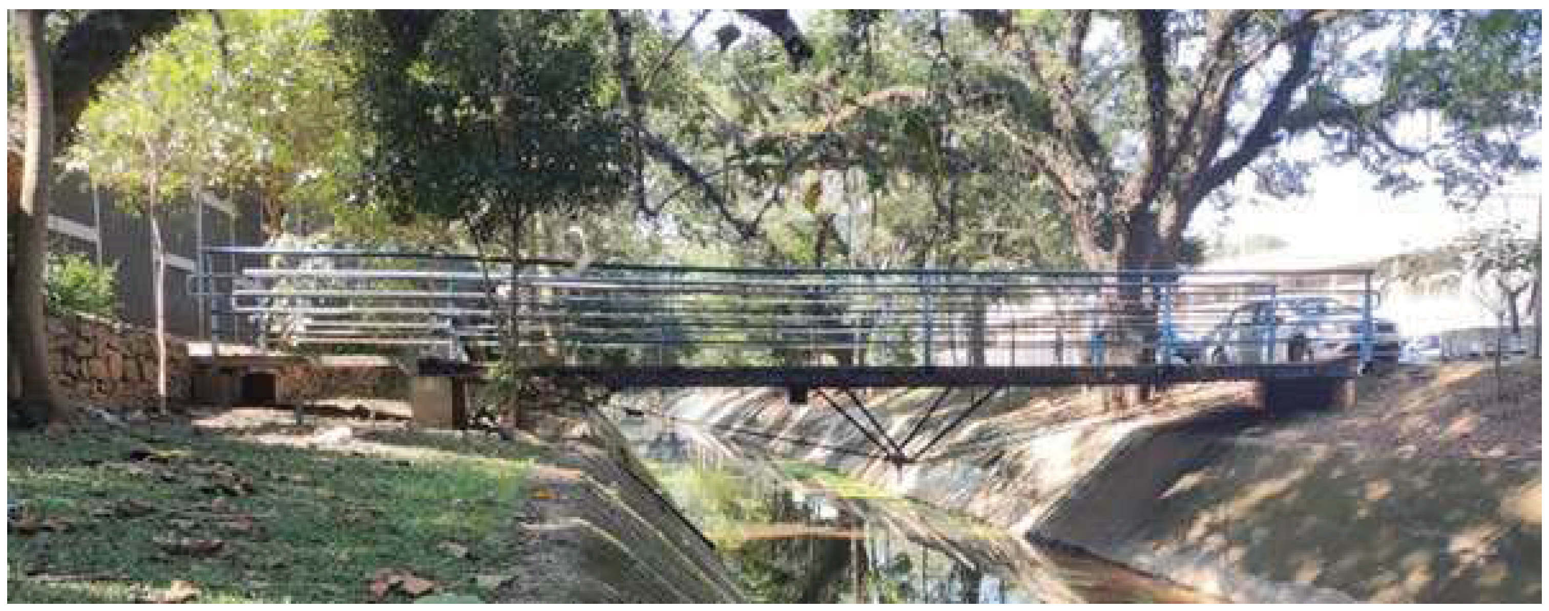
Figure 2.
Construction details and embedded sensors position on the LOP bridge ().
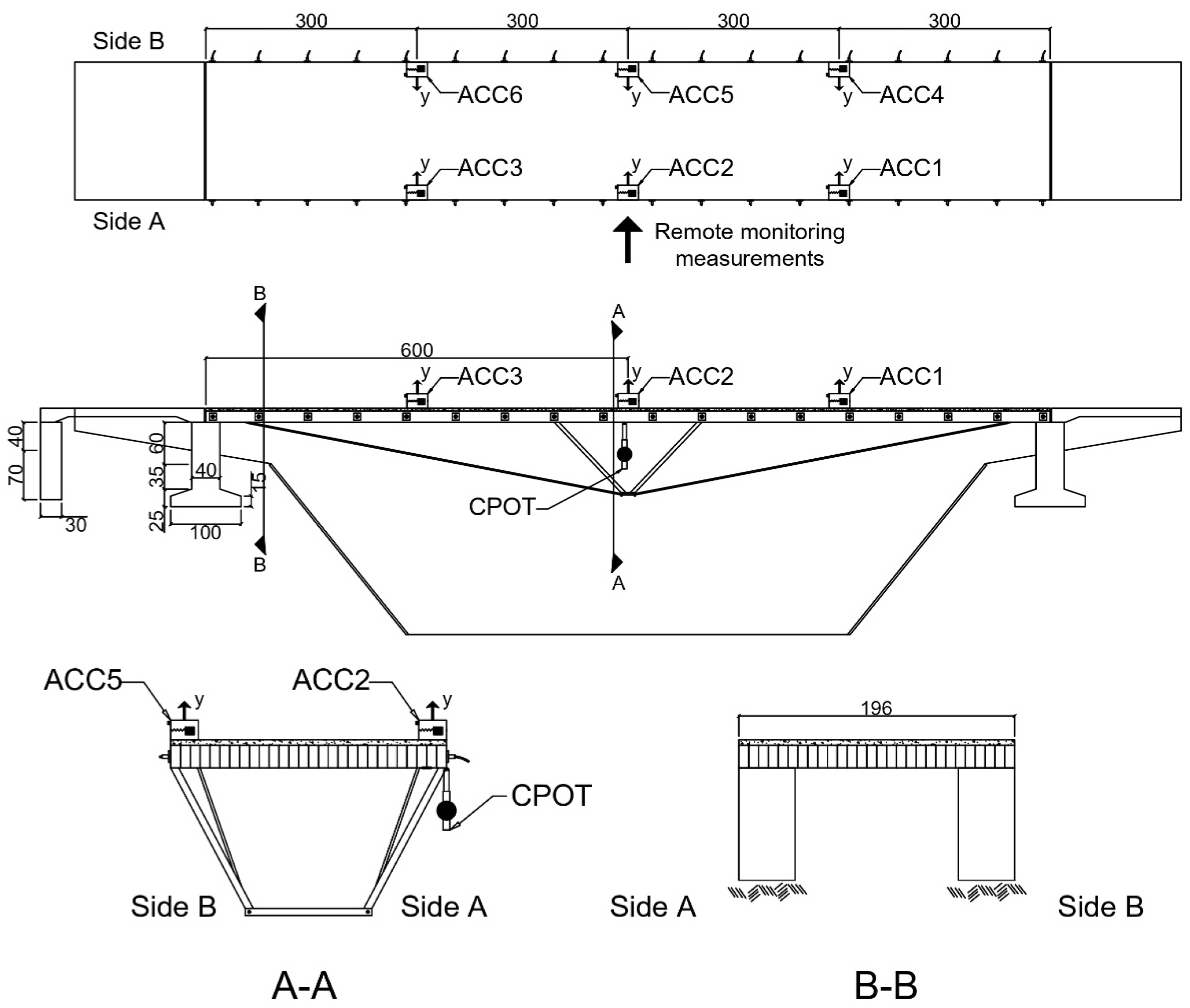
Figure 3.
Geotechnical test for the LOP bridge soil: (a) experiments position, (b) shear modulus and shear wave velocity graphs.
Figure 3.
Geotechnical test for the LOP bridge soil: (a) experiments position, (b) shear modulus and shear wave velocity graphs.
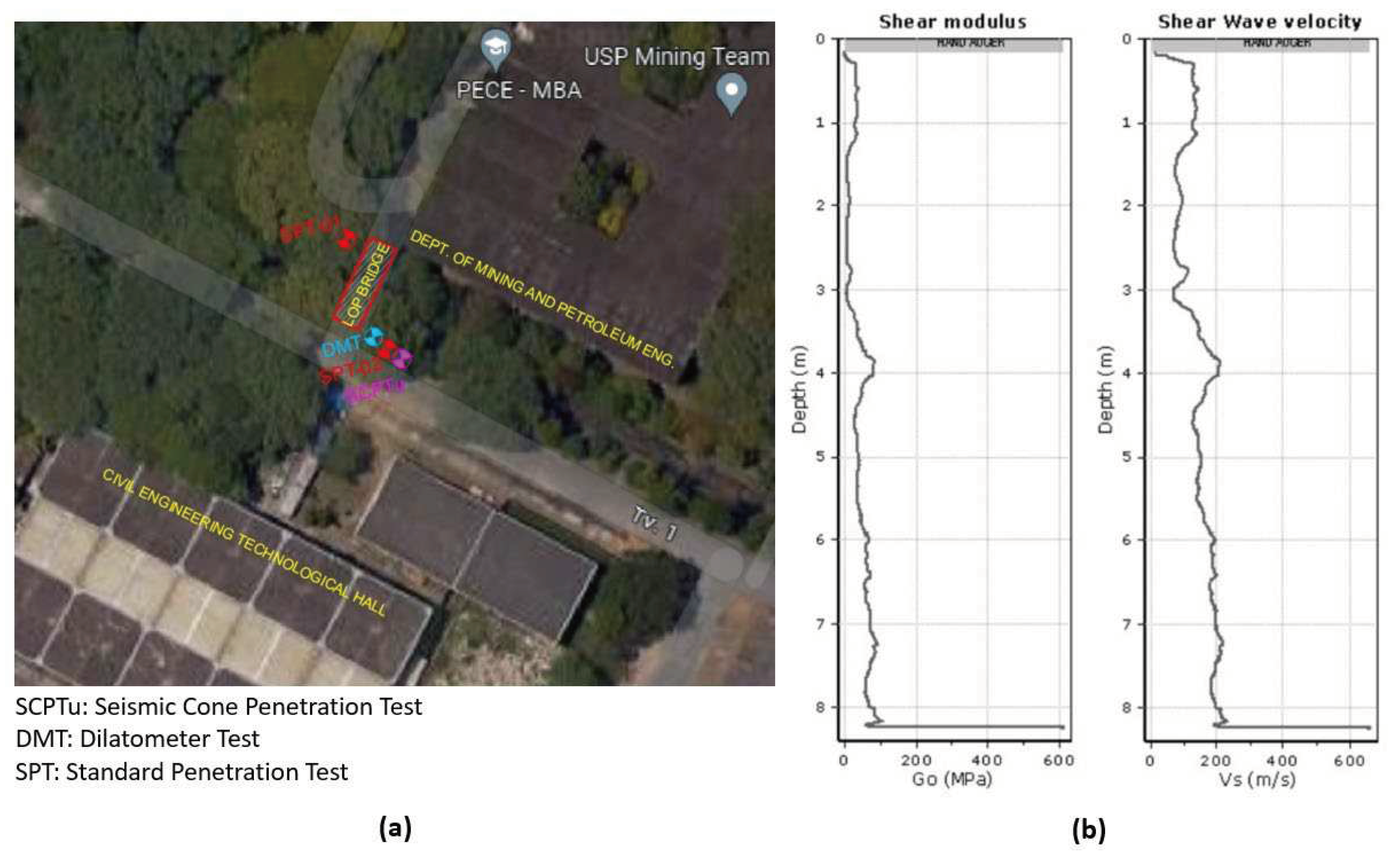
Figure 4.
Displacement transducer installation: (a) CPOT positioned on the LOP slab; (b) installation process detail (Adapted from Teixeira [20]).
Figure 4.
Displacement transducer installation: (a) CPOT positioned on the LOP slab; (b) installation process detail (Adapted from Teixeira [20]).
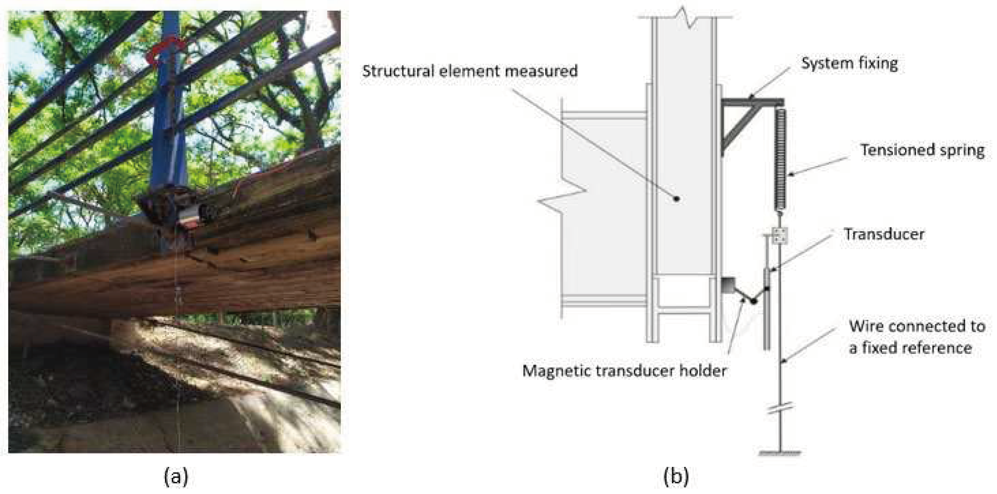
Figure 5.
GBRI positioning.
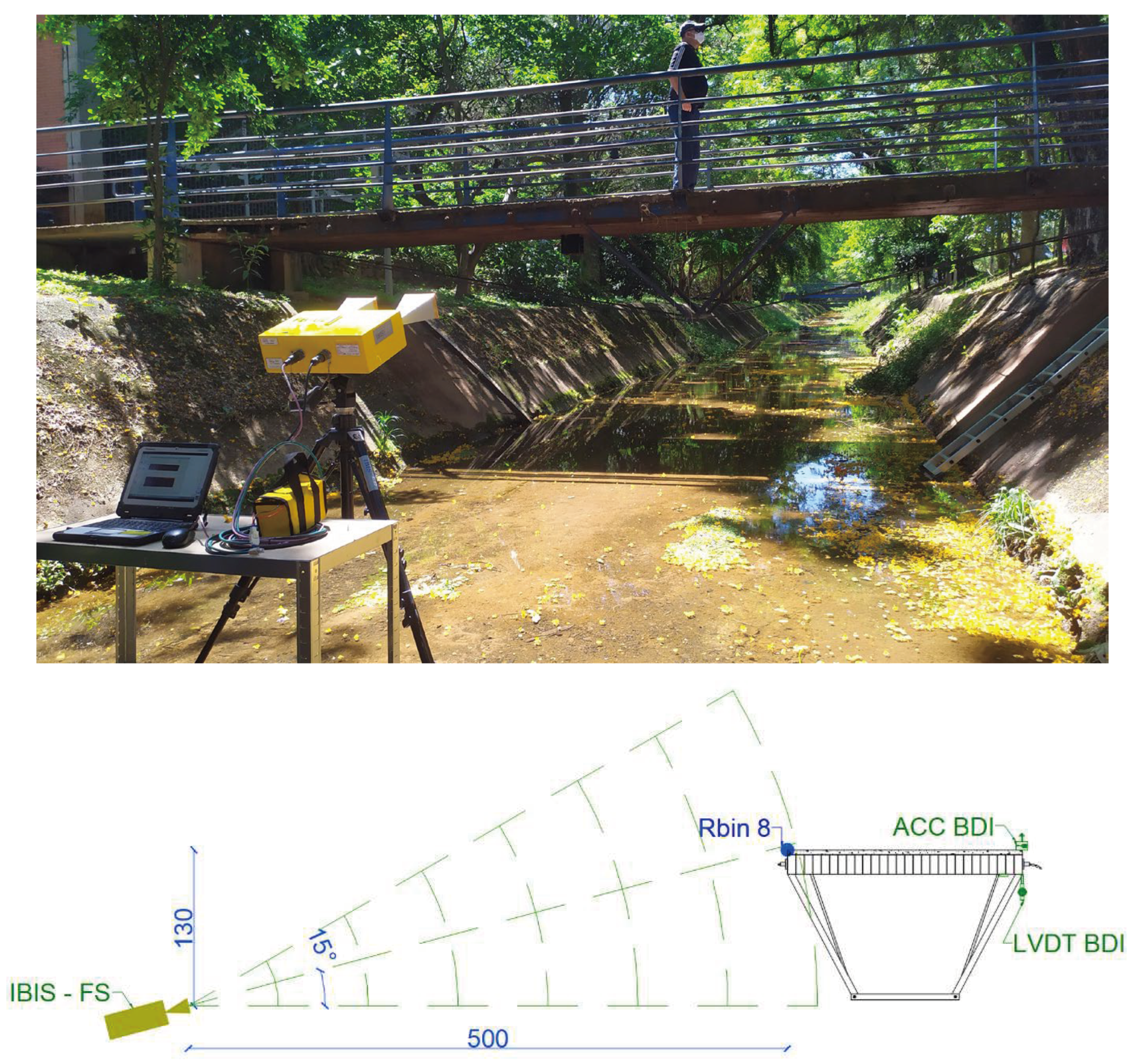
Figure 6.
IBIS-FS range resolution (Quirke and Barrias [22]).
Figure 6.
IBIS-FS range resolution (Quirke and Barrias [22]).
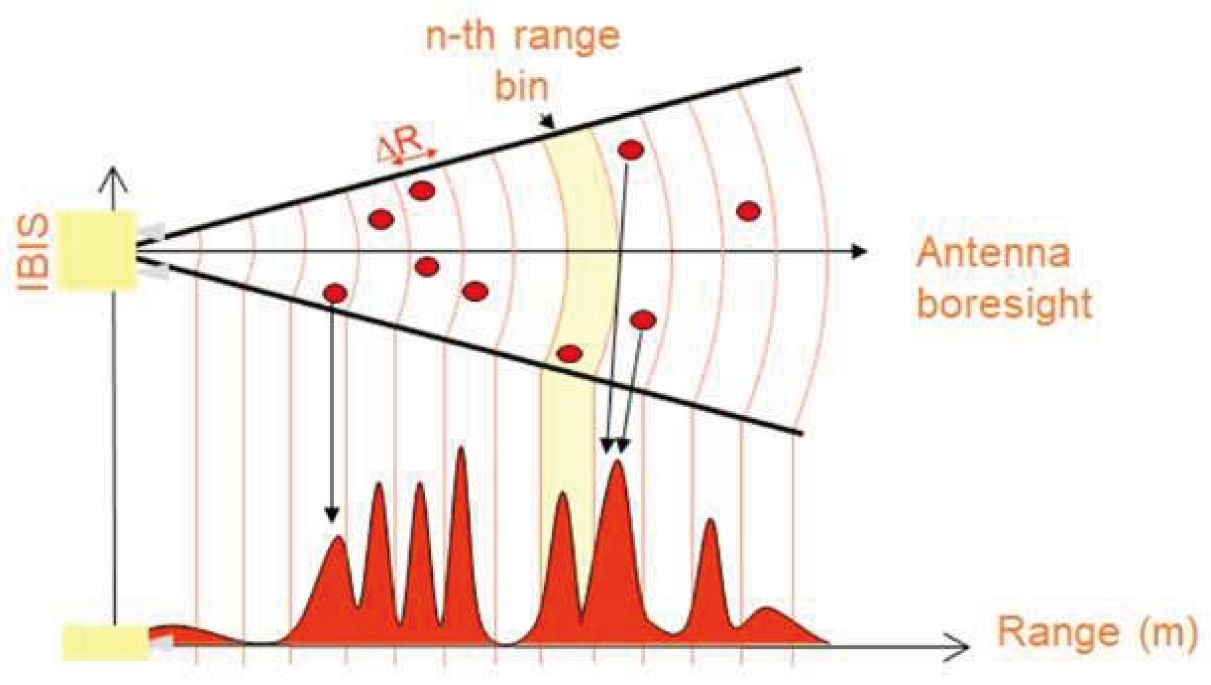
Figure 7.
IRIS-M position.
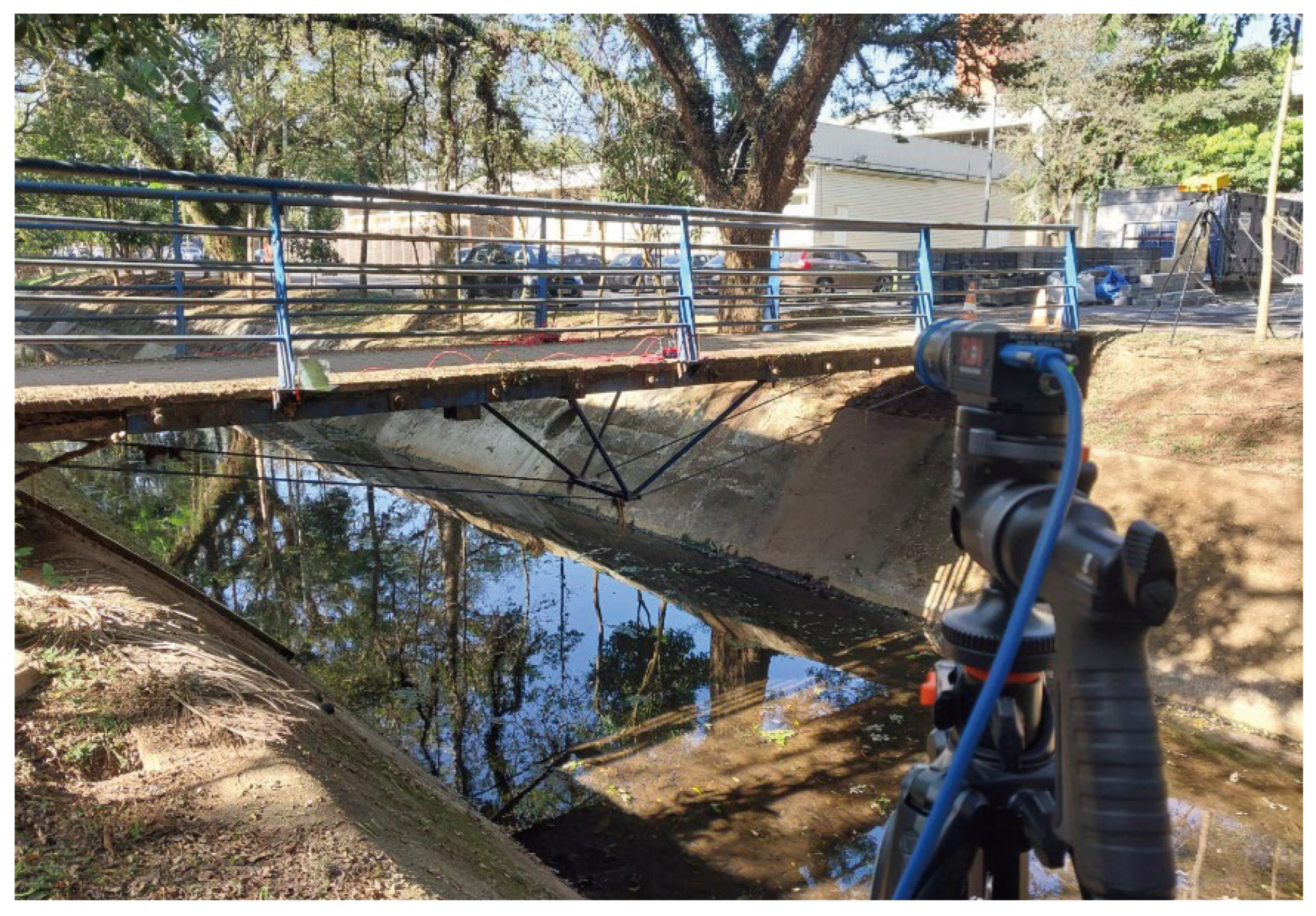
Figure 8.
Contactless motion amplification responses in LOP bridge.
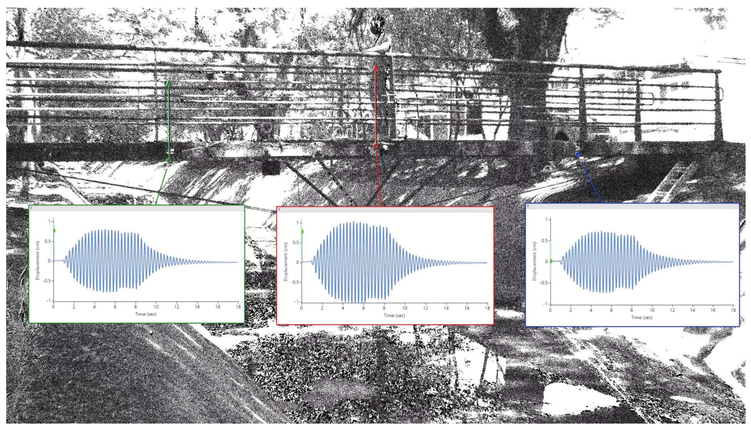
Figure 9.
Load steps (LS) related to the dynamic analysis on the LOP bridge for Test 1.
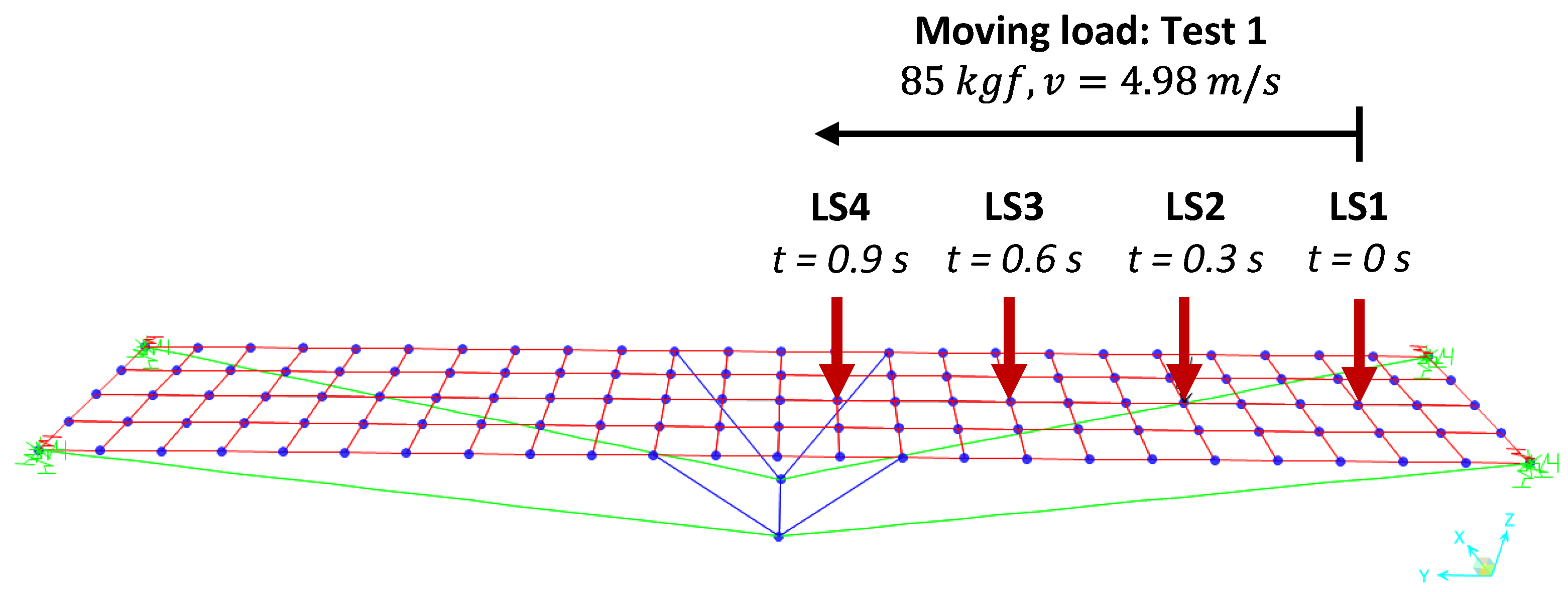
Figure 10.
Loading condition for Test 2 simulation.
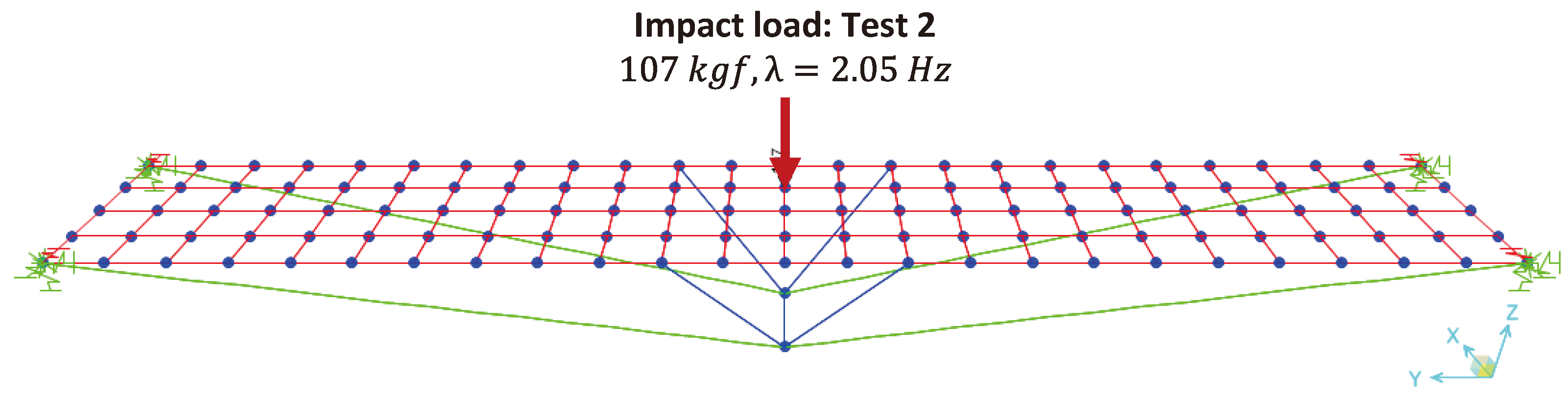
Figure 11.
Heavy-cart moving load configuration employed in Test 3 (dimension in “cm” and load in “kg”).
Figure 11.
Heavy-cart moving load configuration employed in Test 3 (dimension in “cm” and load in “kg”).
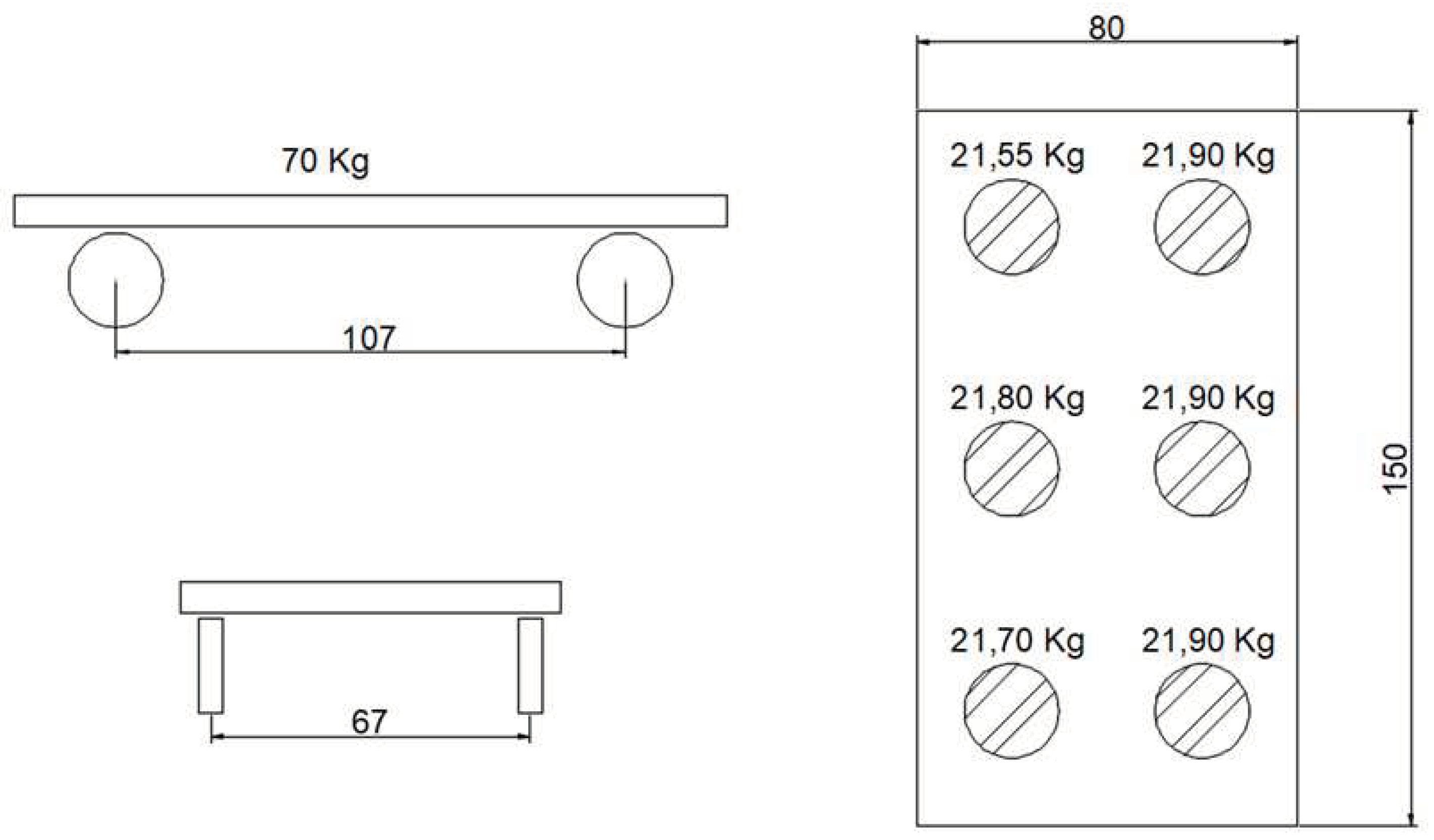
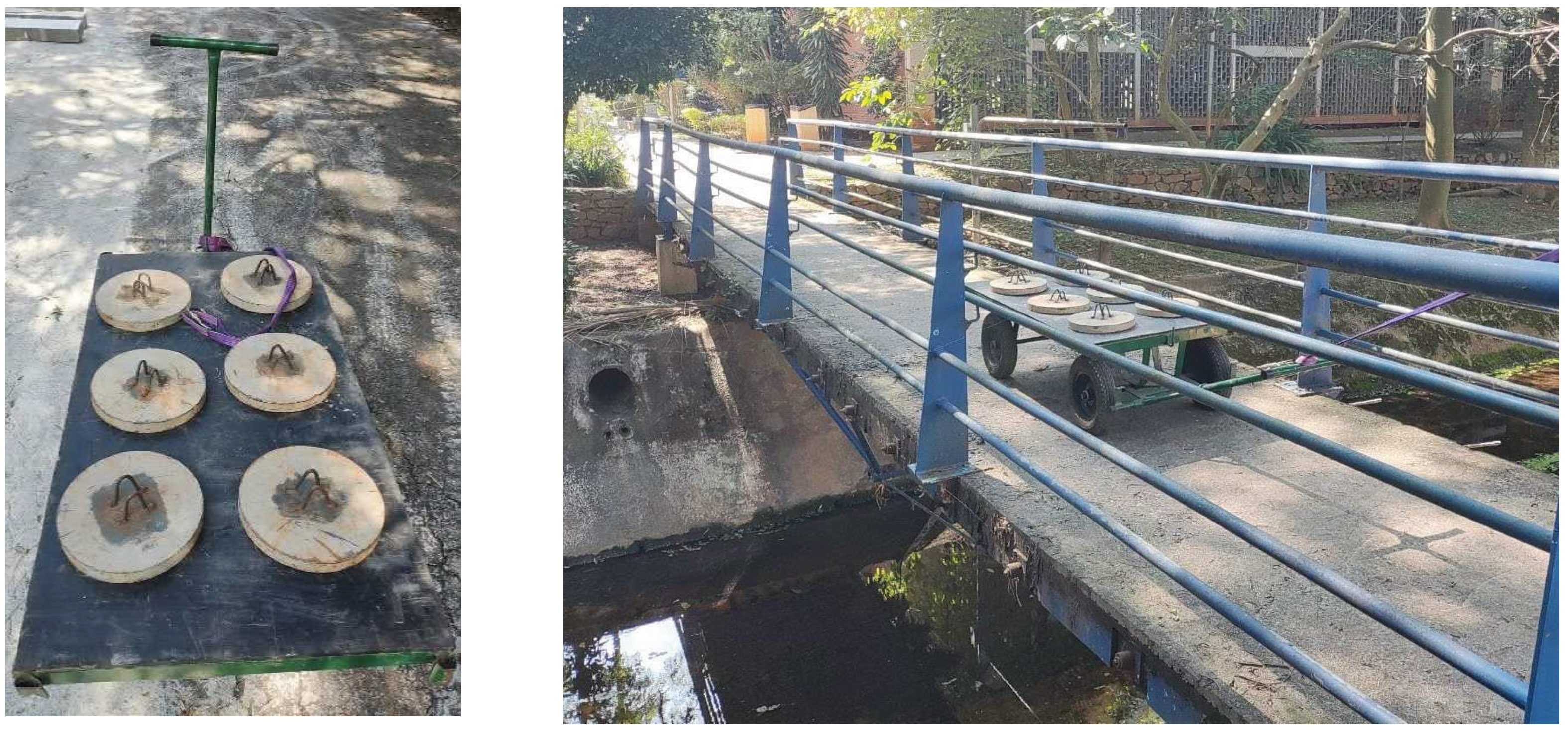
Figure 12.
Lane configuration proposed for the finite element model.
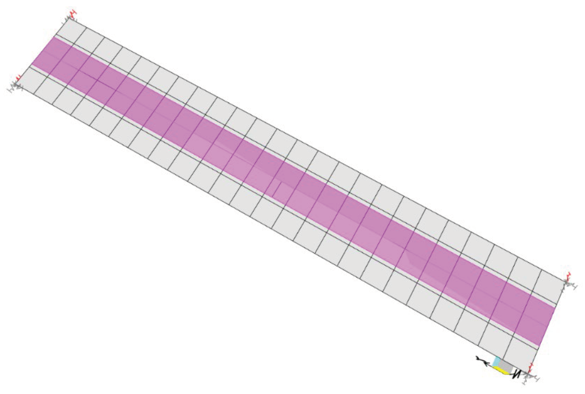
Figure 13.
Displacements measured using LVDT and IBIS-FS for Test 1. .
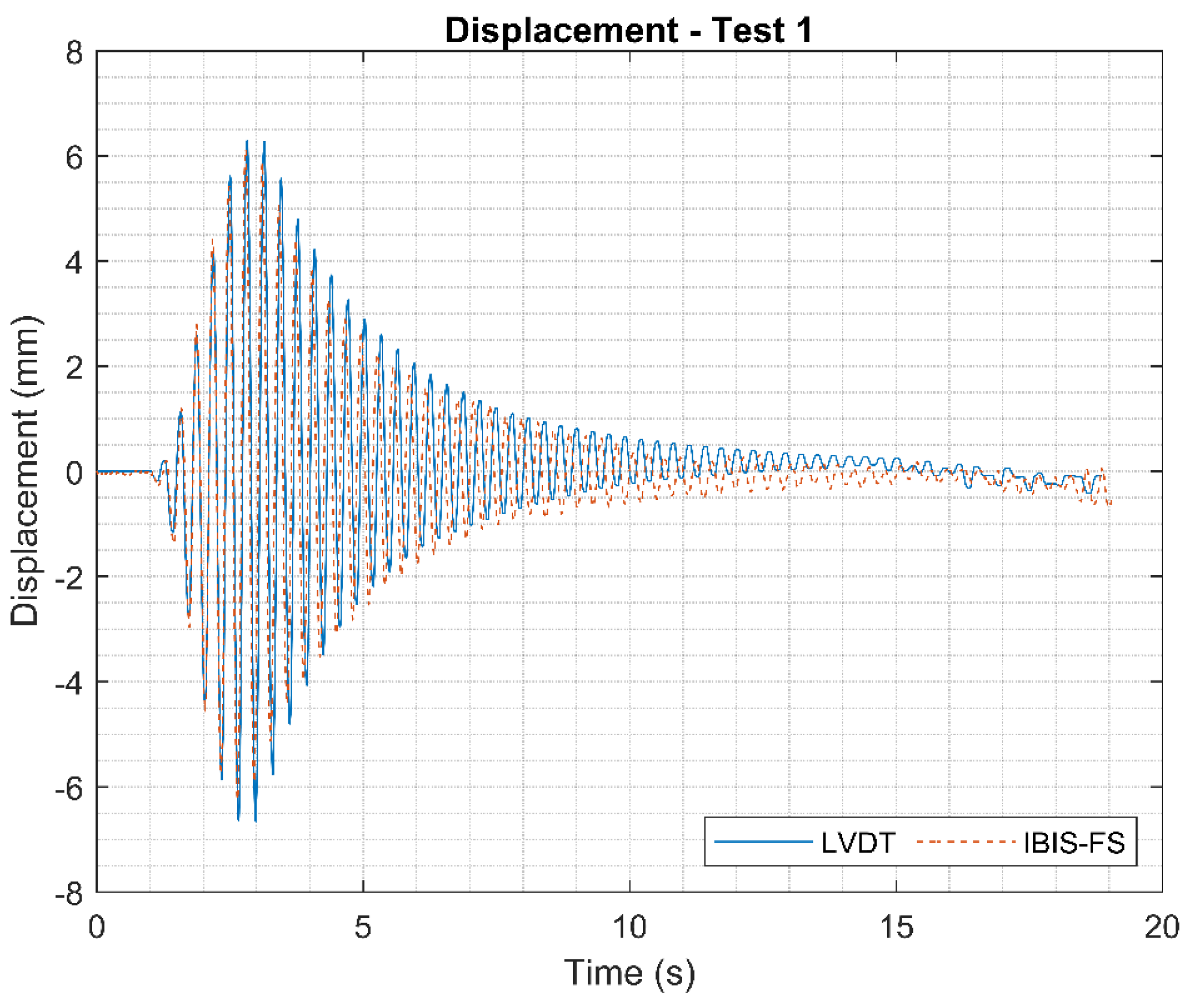
Figure 14.
Accelerations measured in Test 1.
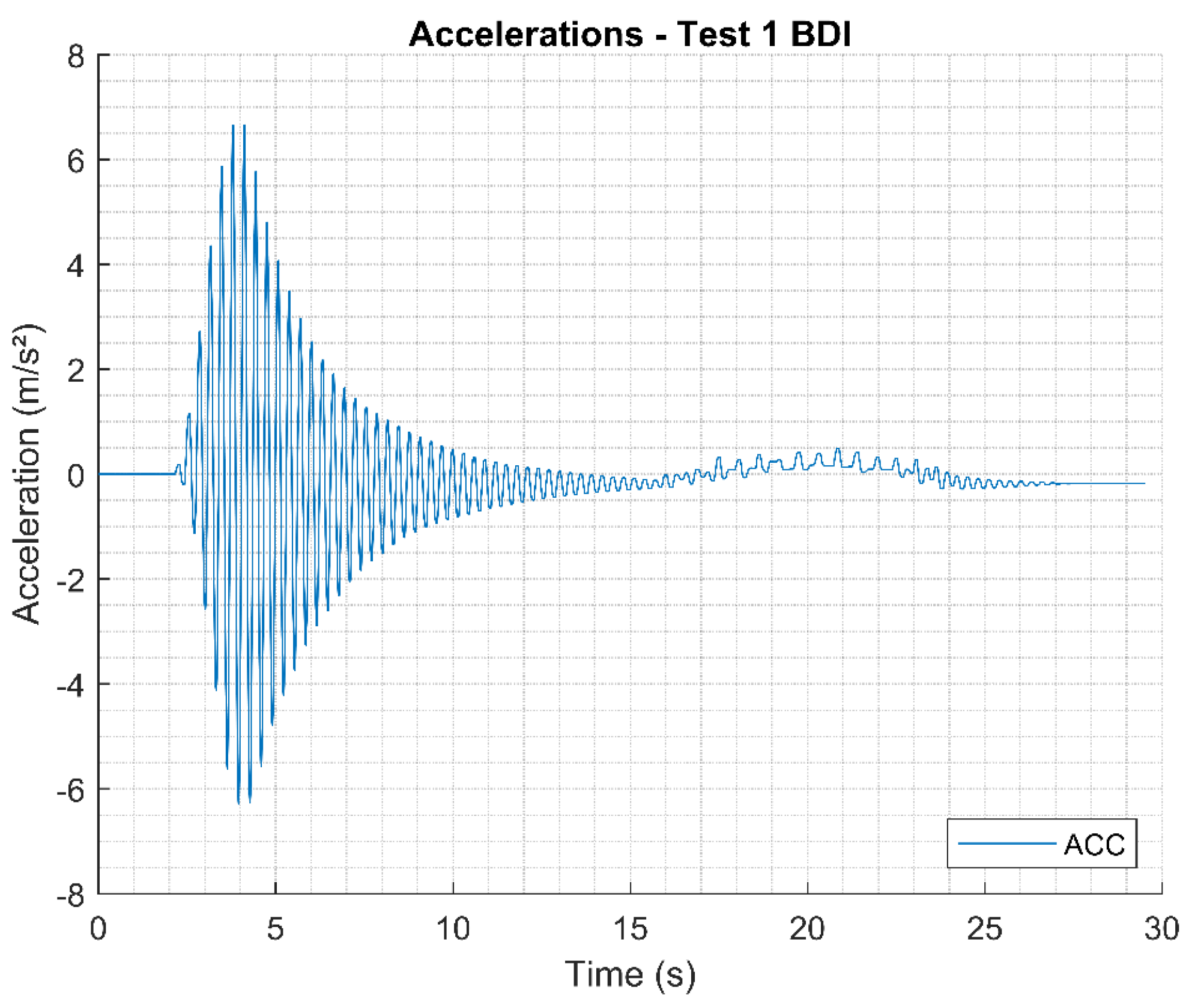
Figure 15.
Displacements measured using LVDT for Test 2.
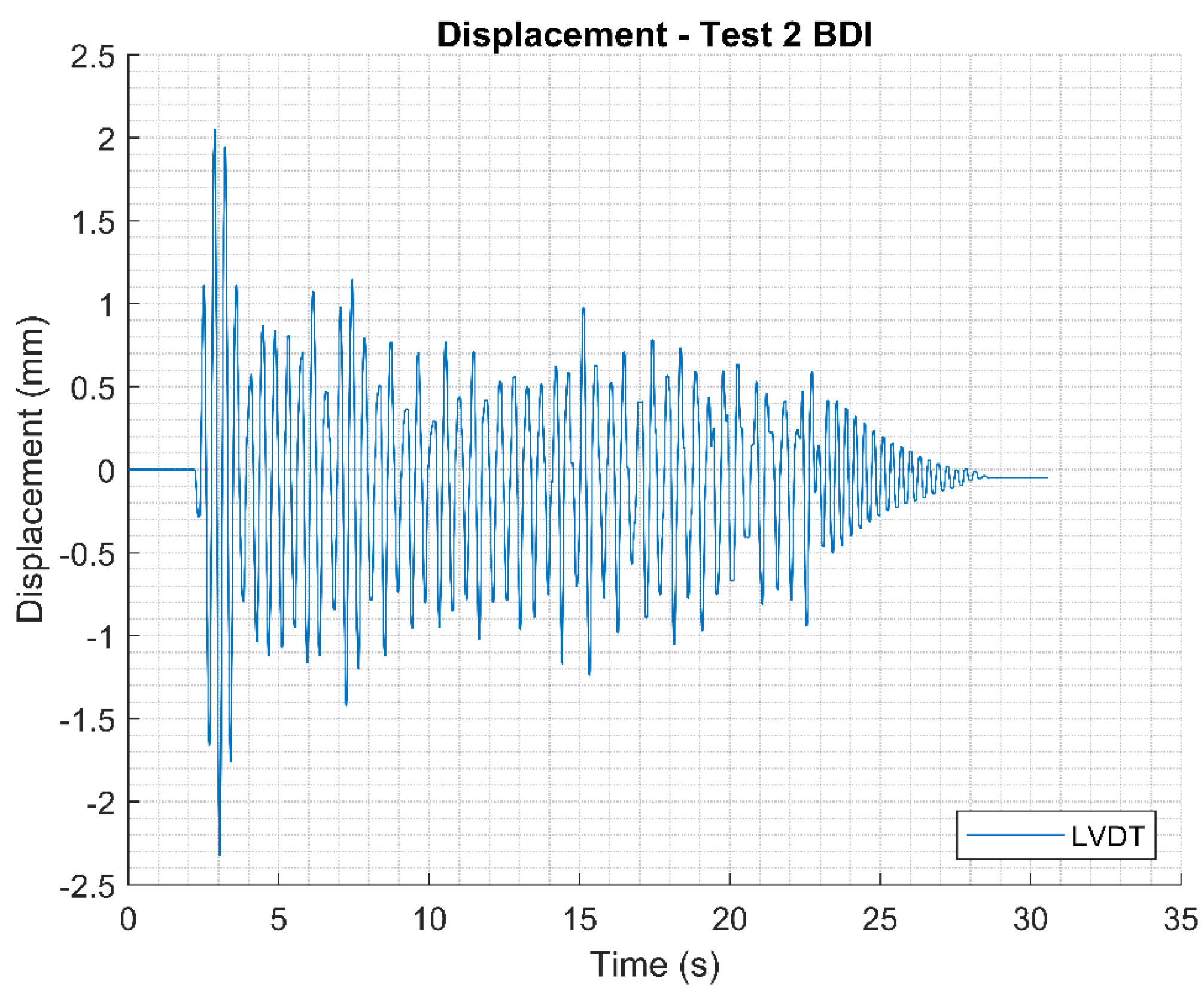
Figure 16.
Accelerations measured in Test 2.
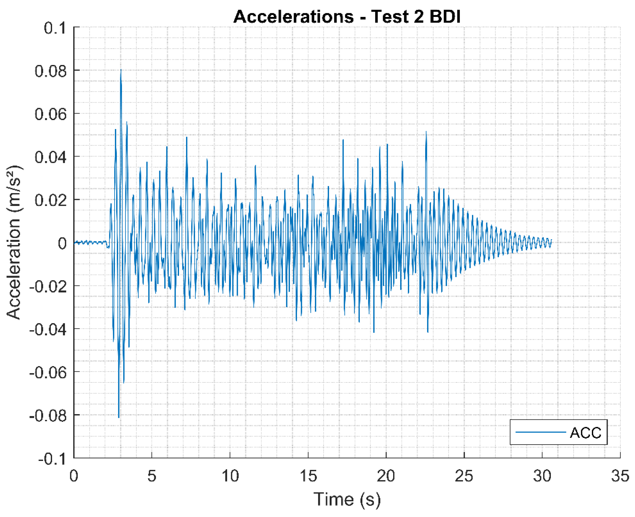
Figure 17.
Displacements measured using IBI-FS for Test 2.
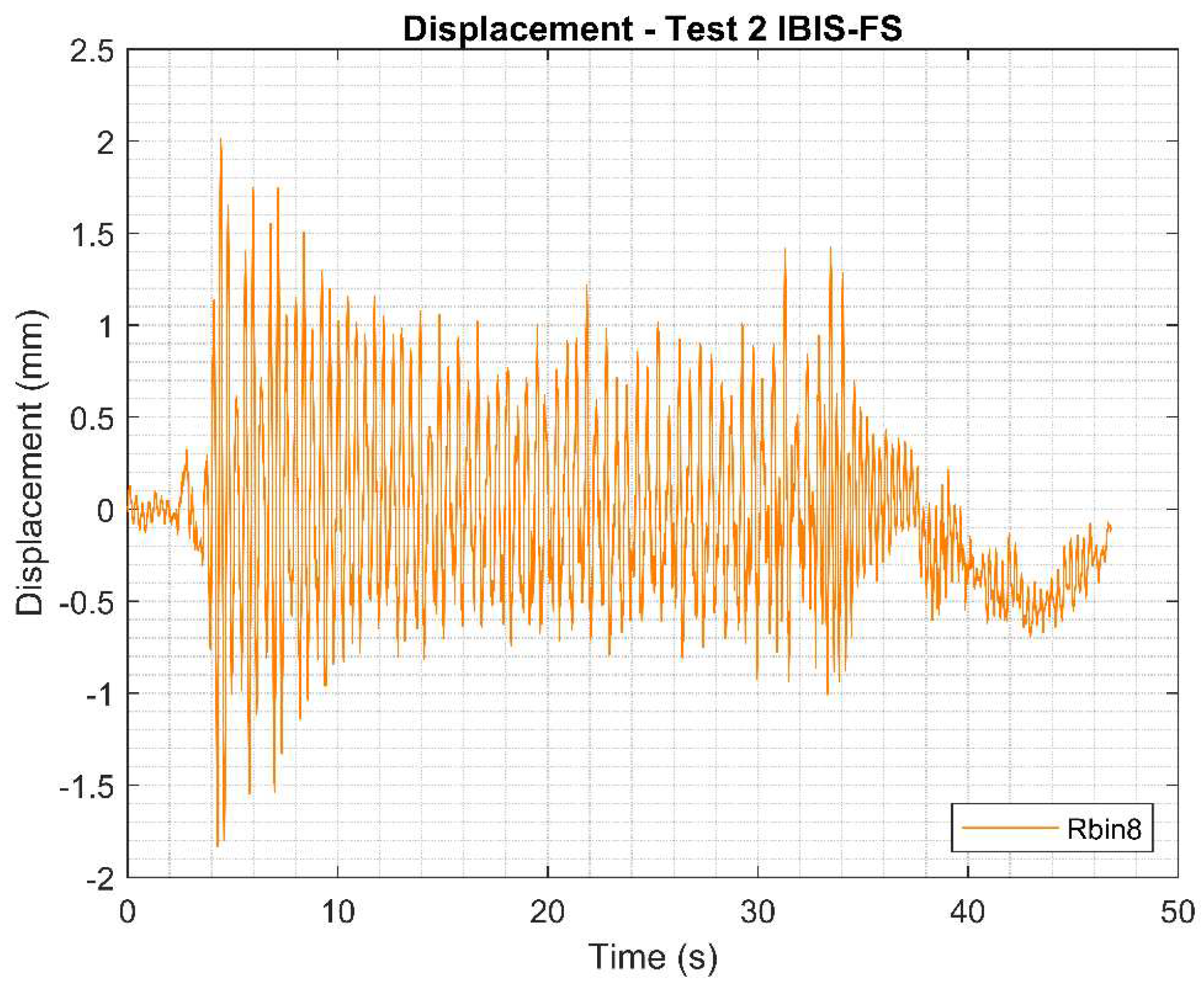
Figure 18.
Displacements measured using LVDT and IBIS-FS for Test 3.
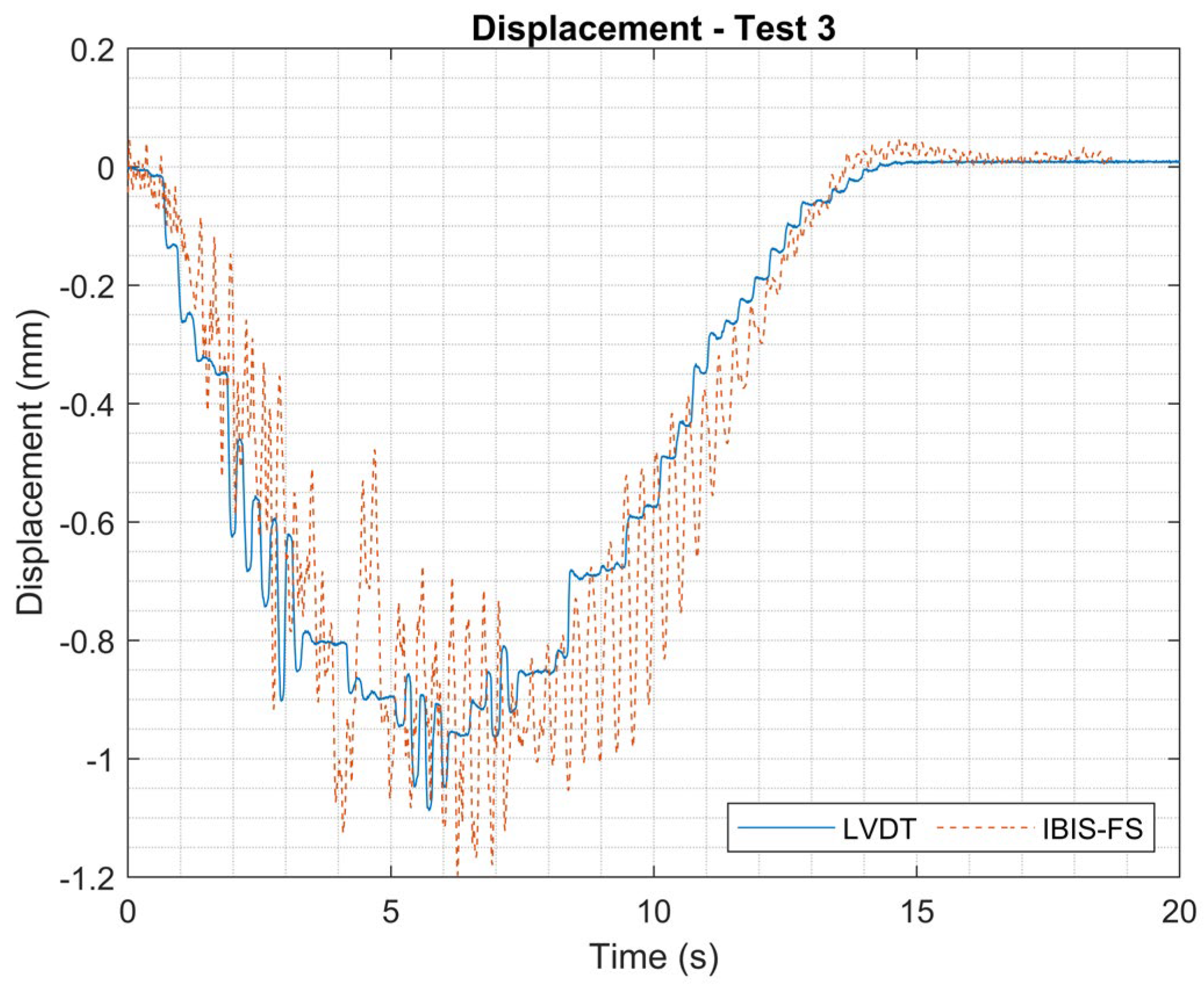
Figure 19.
Experimental frequencies obtained by IBIS-FS and accelerometer data during Test 1.
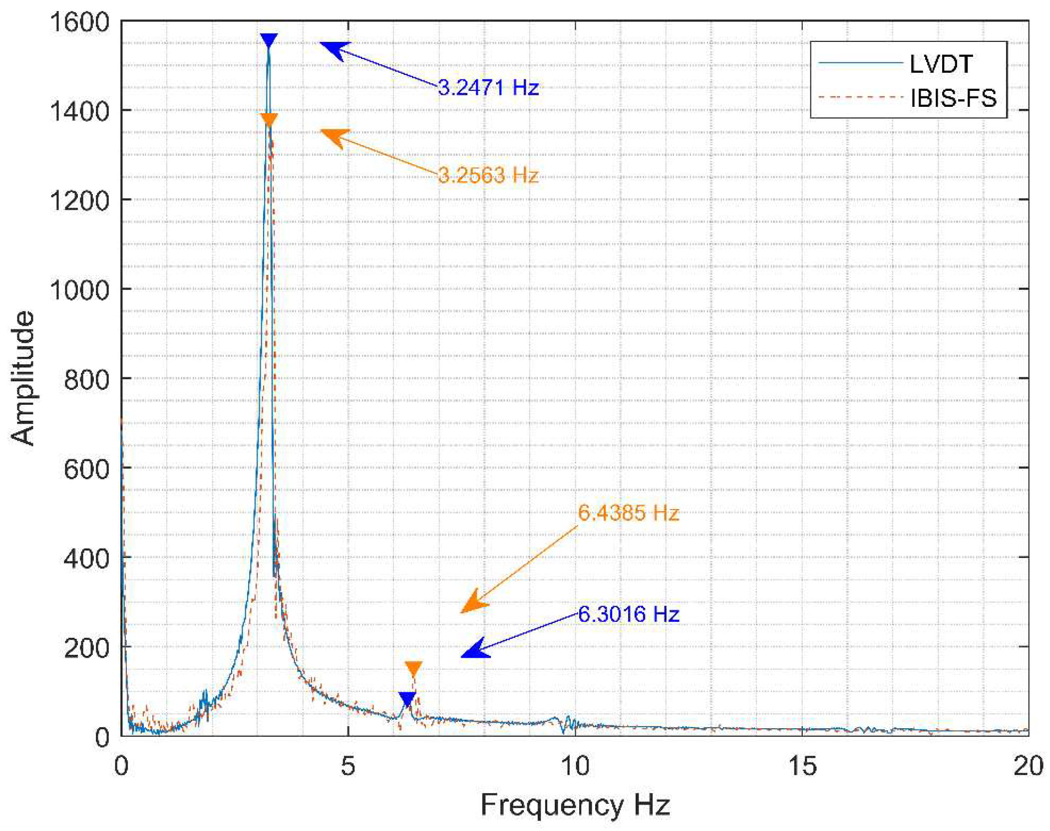
Figure 20.
Consecutive peak values for damping rate calculation .
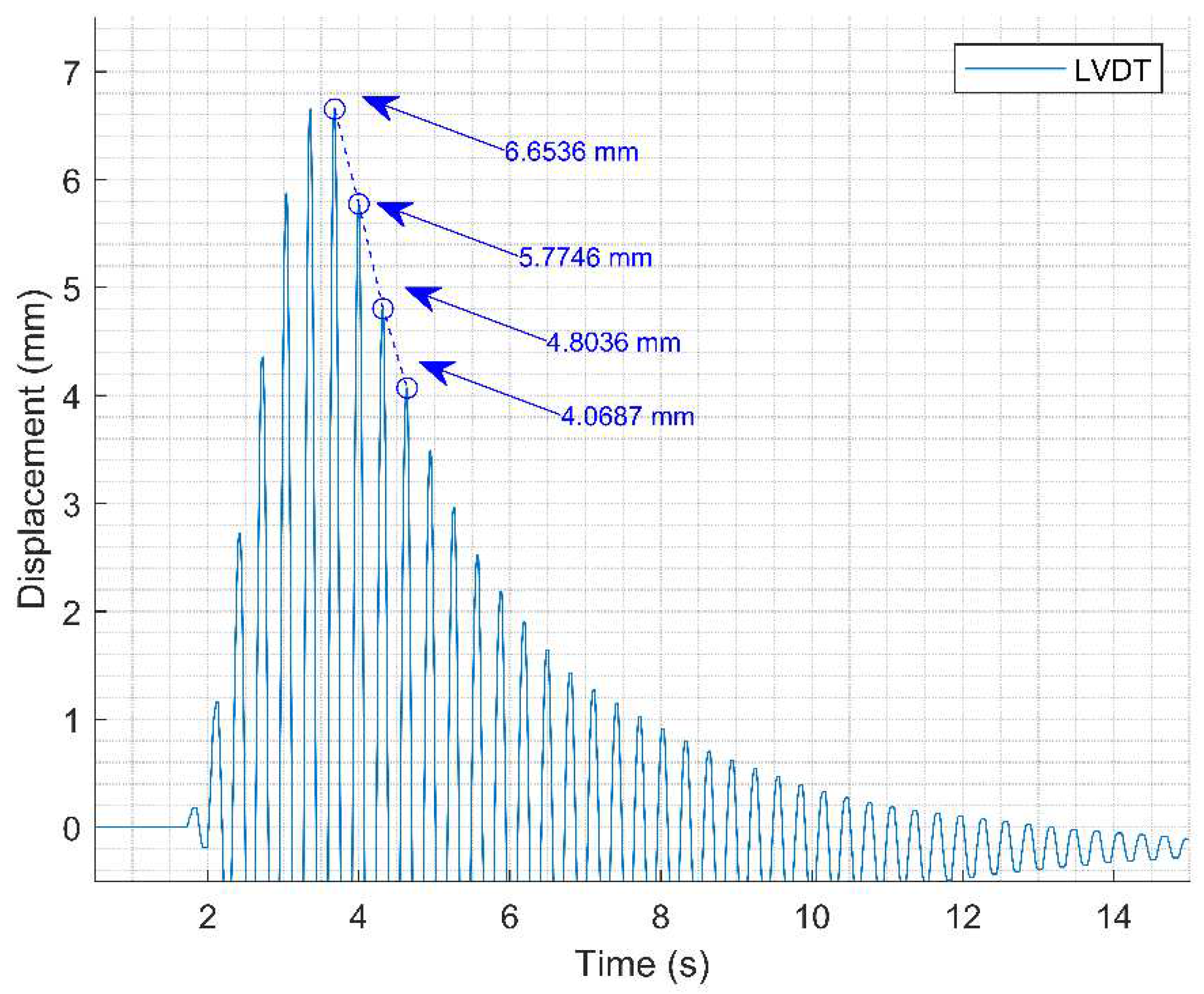
Figure 21.
Results of vertical accelerations on the LOP deck for free vibration Test 1.
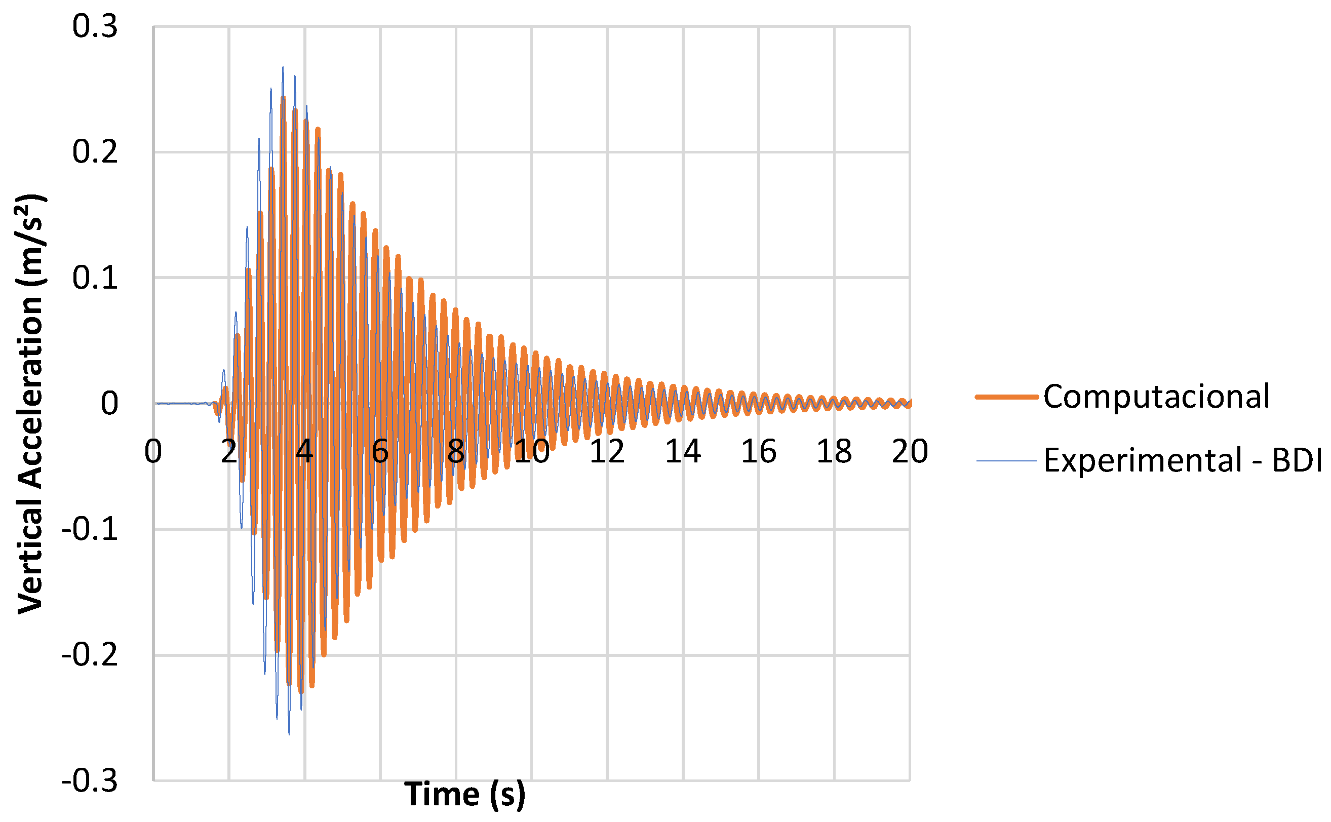
Figure 22.
Numerical results for dynamic Test 1 in LOP.
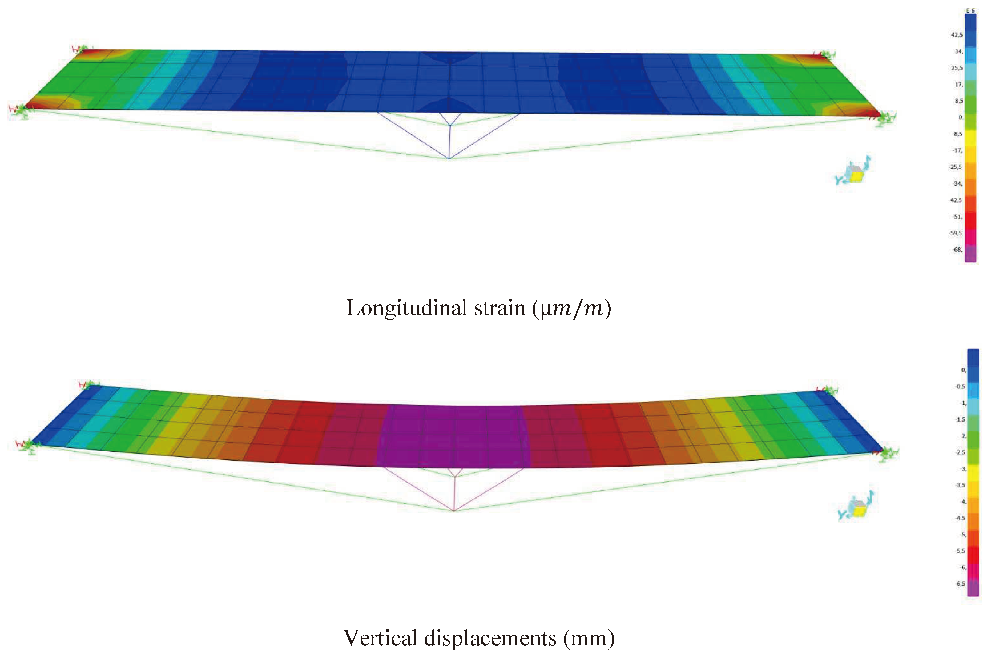
Figure 23.
Numerical results of vertical accelerations on the LOP deck for free vibration Test 1.
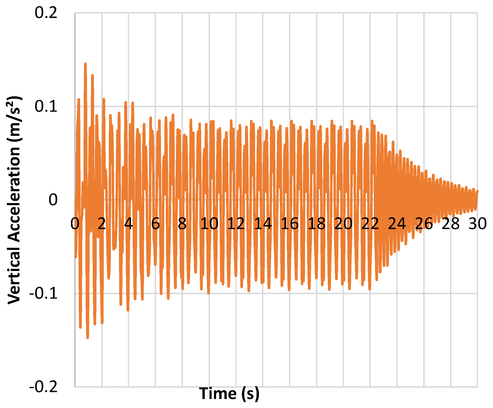
Figure 24.
Computational results for dynamic Test 2 in LOP.
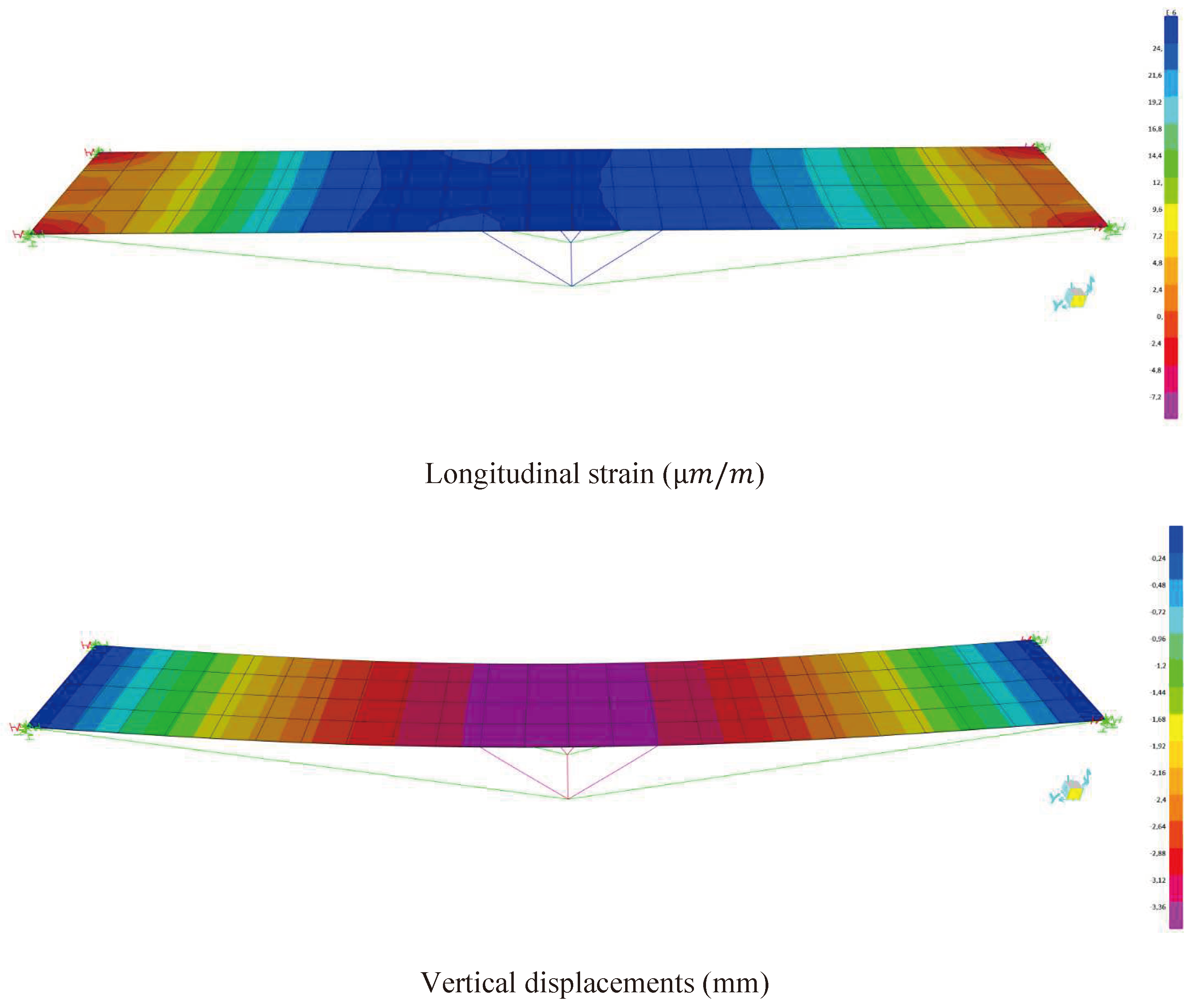
Figure 25.
Experimental results for dynamic Test 3 in LOP.
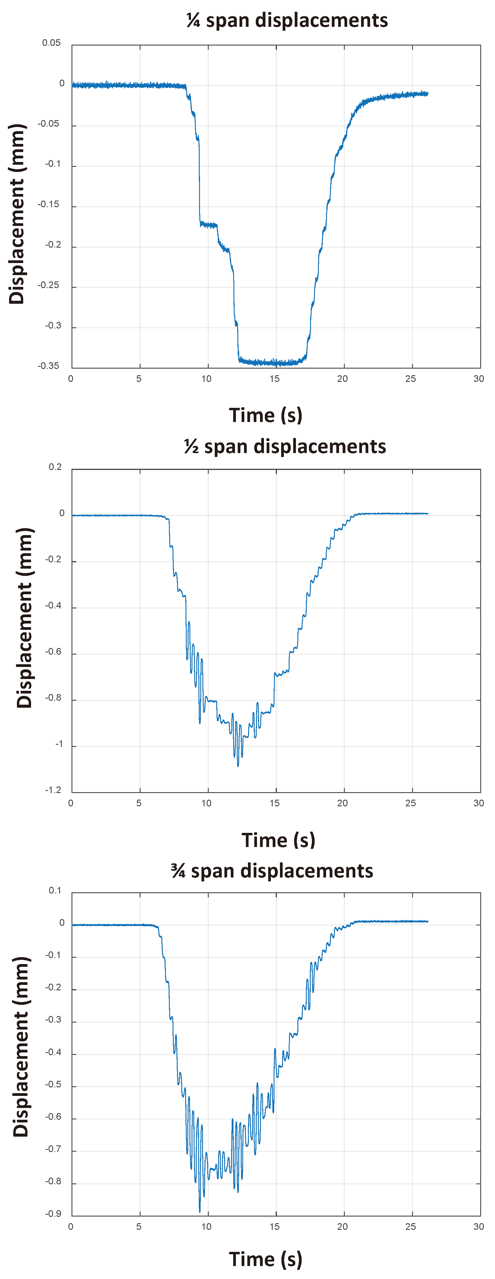
Figure 26.
Vertical computational displacements in “mm” for the Test 3.
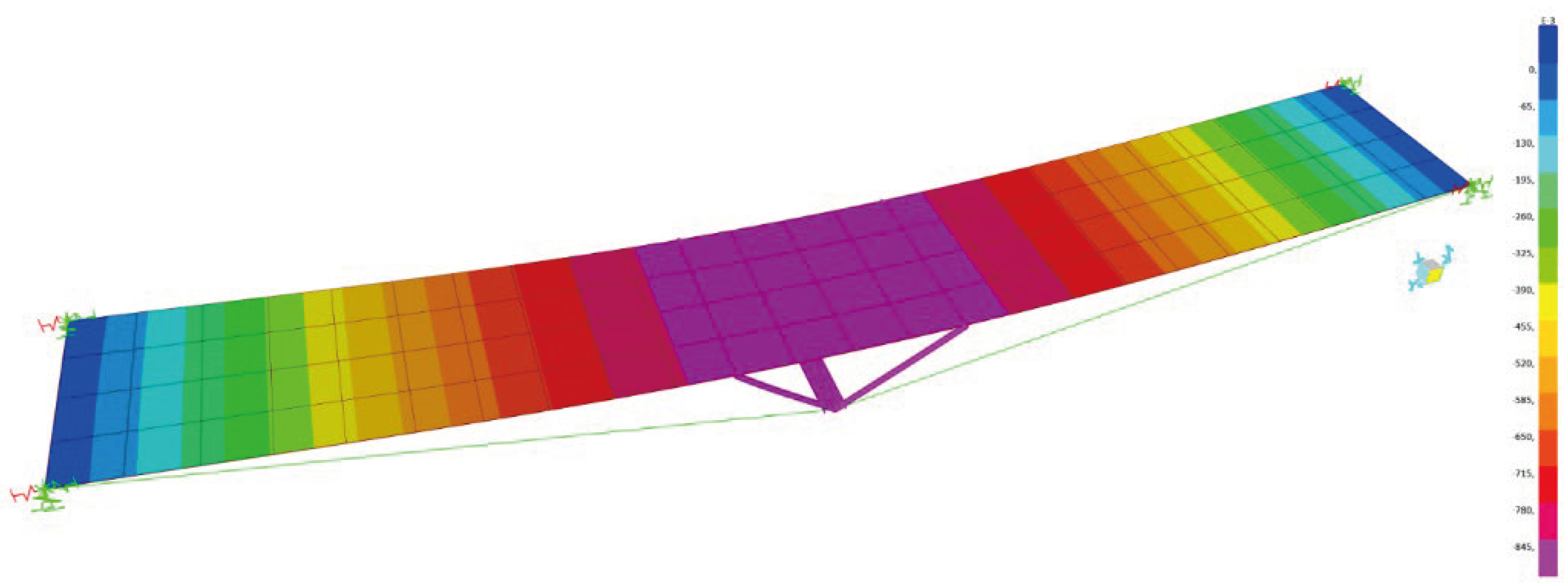
Figure 27.
Estimated modes: (a) Stabilization diagram of estimated state space models and (b) experimental modal configurations.
Figure 27.
Estimated modes: (a) Stabilization diagram of estimated state space models and (b) experimental modal configurations.
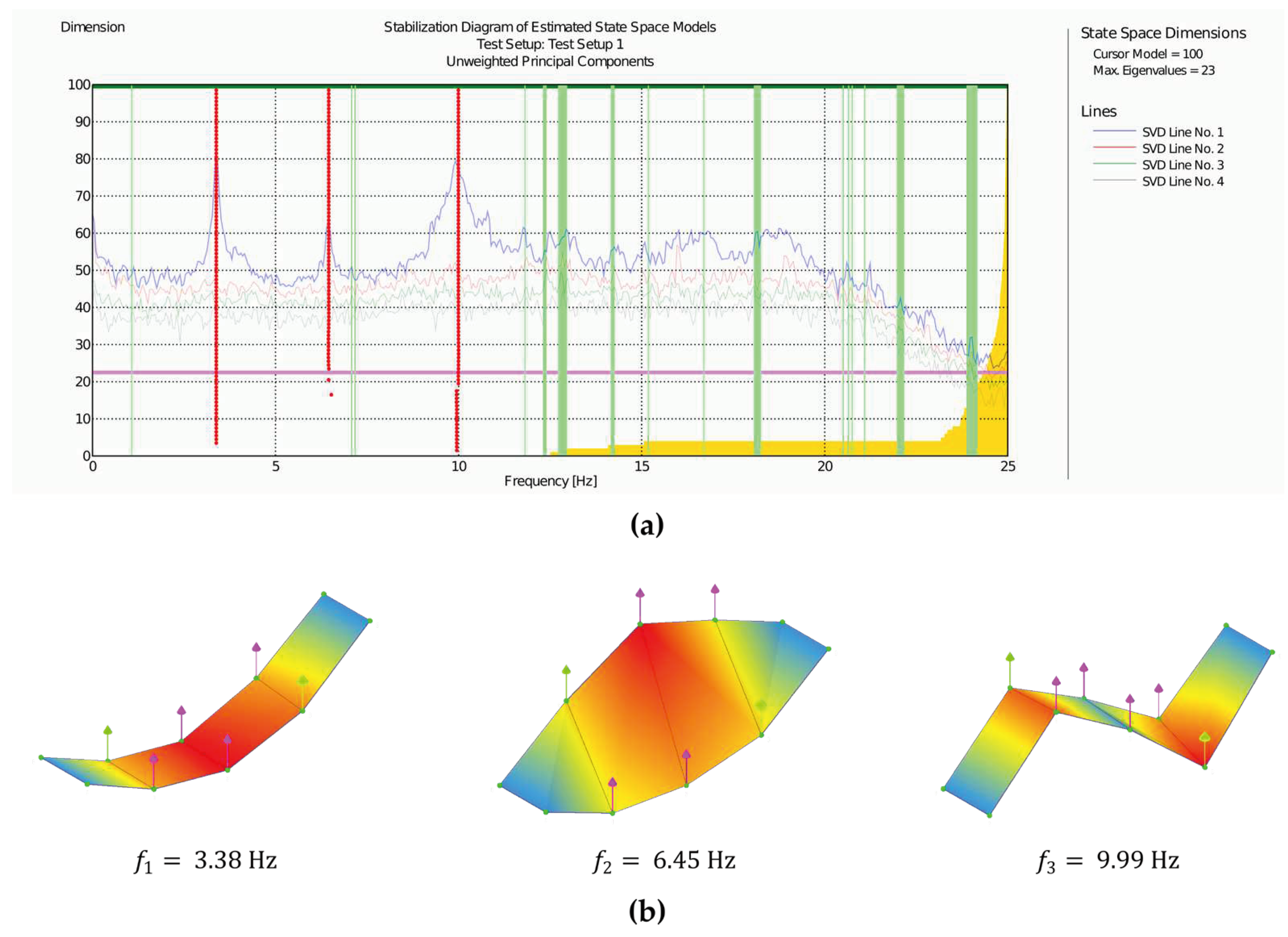
Figure 28.
Asset numerical vibration modes.
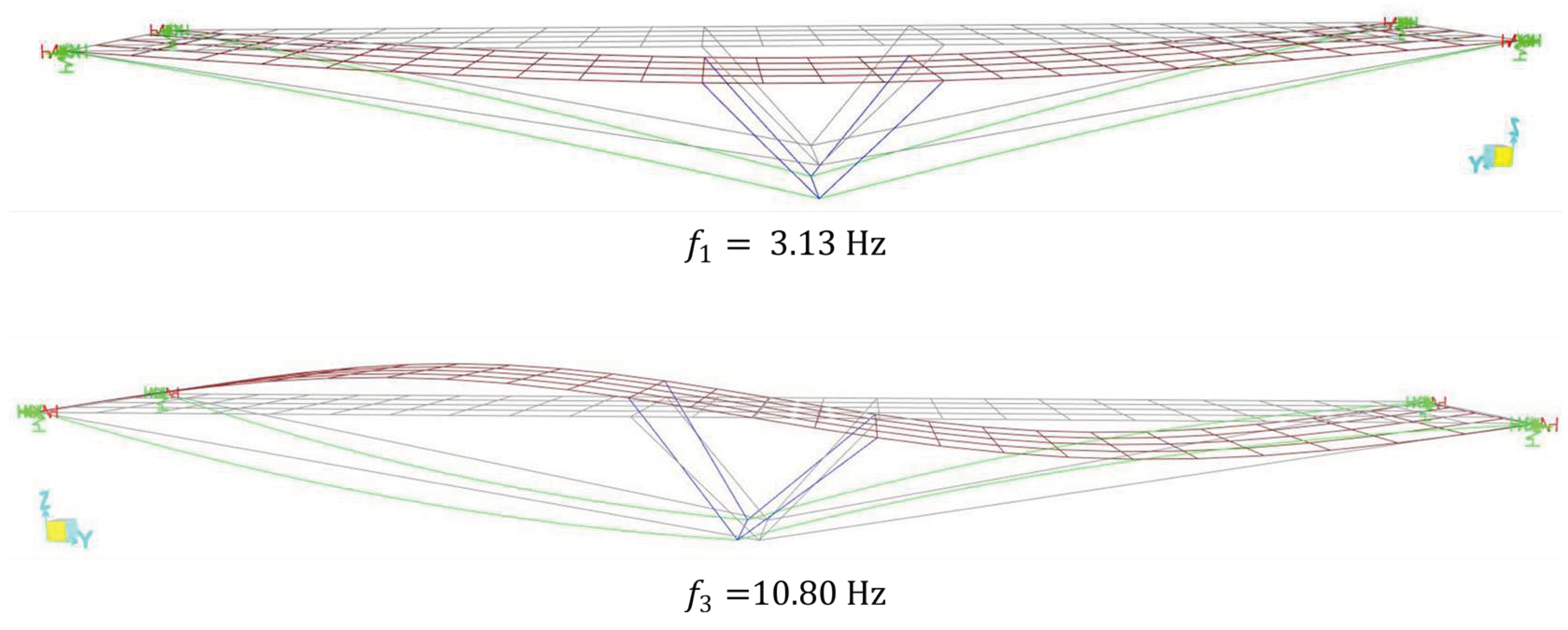

Table 1.
Mechanical material LOP properties.
| Part of the Asset | Attribute Values |
|---|---|
| RC deck | |
| CP 150 RN cables | |
| Wood deck | |
| Tubular and U steel profiles | |
| Soil and foundation (static) | |
| Soil and foundation (Test 1: dynamic free vibration) | |
| Soil and foundation (Test 2: dynamic forced vibration) | |
| Soil and foundation (Test 3: dynamic heavy-load cart moving load) |
Table 2.
Comparison between experimental and computational results for dynamic loads in Test 1.
| Technique | ) | ) |
|---|---|---|
| Numerical | 6.76 | 37.28 |
| Experimental | 6.55 | 30.26 |
* Tables may have a footer.
Table 3.
Comparison between experimental and computational results for dynamic loads in Test 2.
| Technique | ) | ) |
|---|---|---|
| Computational | 3.60 | 23.26 |
| Experimental | 3.25 | 24.90 |
* Tables may have a footer.
Table 4.
Comparison between experimental and numerical results for dynamic loads in Test 3.
| Technique | ) | ) | ) | ) |
|---|---|---|---|---|
| Numerical | 0.91 | 0.629 | 0.629 | 0.629 |
| Experimental (BDI) | 1.09 | 0.348 | 0.890 | 0.619 |
| Experimental (IBIS) | 1.200 | 0.742 | 1.111 | 0,927 |
| Experimental (RDI) | 0.914 | 0.429 | 1.050 | 0,740 |
* Tables may have a footer.
Table 5.
Comparison between experimental and computational results for natural frequencies.
| Flexural Vibration Mode | Experimental | Numerical | Deviation [%] |
|---|---|---|---|
| Mode I (Hz) | 3.38 | 3.13 | 7 |
| Mode II (Hz) | 9.99 | 10.80 | 8 |
Disclaimer/Publisher’s Note: The statements, opinions and data contained in all publications are solely those of the individual author(s) and contributor(s) and not of MDPI and/or the editor(s). MDPI and/or the editor(s) disclaim responsibility for any injury to people or property resulting from any ideas, methods, instructions or products referred to in the content. |
© 2023 by the authors. Licensee MDPI, Basel, Switzerland. This article is an open access article distributed under the terms and conditions of the Creative Commons Attribution (CC BY) license (http://creativecommons.org/licenses/by/4.0/).
Copyright: This open access article is published under a Creative Commons CC BY 4.0 license, which permit the free download, distribution, and reuse, provided that the author and preprint are cited in any reuse.


