
Submitted:
10 November 2023
Posted:
14 November 2023
You are already at the latest version
Abstract
Ca Mau Peninsula (CMP), the southernmost region of the Mekong Delta, is facing a severe loss of land and freshwater. Particularly, the groundwater resources in the complex multilayered aquifer system of CMP are subject to salinization processes, which are not yet fully understood. In this study, an existing groundwater flow model for the CMP was enhanced to a density-dependent transient transport model using the FEFLOW software package, which is based on the finite element method. The study focuses on simulating groundwater salinity in order to better understand the dynamics of groundwater salinization and potential saltwater intrusion pathways in the study area. Time series of Total Dissolved Solids (TDS) concentrations at observation wells were used to compare simulated and observed salinity data in different aquifers. The model allows a multi-factorial evaluation of the spatial groundwater salinity and could also confirm significant inter-annual variability, particularly in the case of shallow aquifers due to the influence of tides and seasonal rainy/dry seasons. Using sensitivity analysis, leakage from upper saline aquifers into lower freshwater aquifers through natural hydrogeological windows and poorly sealed boreholes was identified as a potential major cause for groundwater salinization occurring in the region. The results obtained can serve as an important basis for developing decision-making tools to promote the sustainable use of water resources on the CMP in the future.
Keywords:
salinity modeling
; groundwater transport modeling
; hydrogeology
; aquifers system
; Ca Mau
; Kien Giang
; Soc Trang
; Hau Giang
; Bac Lieu
1. Introduction
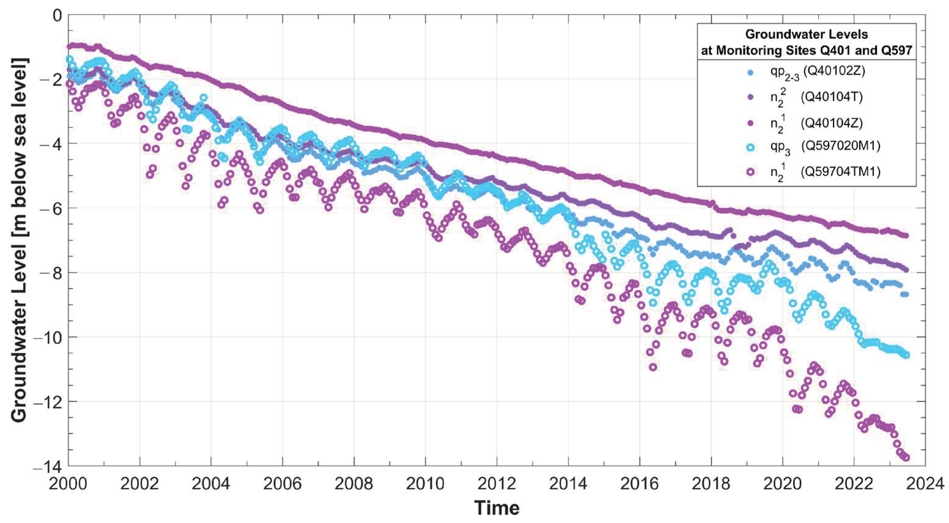
The salinization of groundwater in the southernmost region of the Mekong Delta poses a significant challenge to the local population (UN VIETNAM, 2020). Groundwater is a crucial resource that is used for domestic, agricultural, aquacultural, and commercial purposes (Nhan et al., 2007; Pham et al., 2023). It is predominantly relied upon as the primary freshwater source due to the limited availability of alternative water sources, particularly in remote areas on the Ca Mau Peninsula (CMP) and areas with increased surface water salinity, particularly during the dry season (Bauer et al., 2022). Consequently, excessive exploitation of groundwater has resulted in a decline in groundwater levels (Figure 1).
The hydrogeological setup of the CMP covers seven aquifers and seven aquitards ( Hoan et al., 2022; Vuong et al., 2014), and plays a crucial role in understanding groundwater dynamics as well as saline intrusion. In previous studies, aquitards have often been regarded as continuous formations that act as effective sealing layers. However, recent studies suggest that heterogeneities should be considered (Minderhoud et al., 2017; Wagner et al., 2012). In addition, geochemical signatures across several aquifers indicate a non-neglectable aquifer mixing (Bauer et al., 2023). An evaluation of water levels at monitoring sites with several wells in different aquifers shows that the dynamics of water levels in different aquifers seem to be linked to each other, which suggests that the aquifers may not be separated from each other, but may rather be interconnected. However, also loading effects could explain this synchronized dynamics of groundwater levels in the confined aquifers, as shown for example in the Bengal Basin (Burgess et al., 2017).
Figure 1.
Trend of groundwater level decline in monitoring well groups Q597 and Q401, located in the Ca Mau Peninsula (sources of data: NAWAPI).
Figure 1.
Trend of groundwater level decline in monitoring well groups Q597 and Q401, located in the Ca Mau Peninsula (sources of data: NAWAPI).
Since the beginning of the 21st century, countries upstream of the Mekong River constructed a large number of hydropower dams (Van Khanh Triet et al., 2017) to serve the energy and water demand of agricultural production and other economic activities. This has led to a decrease in water flow from upstream (Allison et al., 2017; Binh et al., 2020; Karlsrud et al., 2017), affecting the livelihoods of people downstream. In addition to the lack of freshwater in the dry season, under the influence of tides, seawater penetrates the surface water bodies inland, leading to saline intrusion in rivers, lakes, and channels, as well as shrimp and rice farming areas.
In response, the Vietnamese government has developed adaptation policies on water resource planning and management (MONRE, 2022). Many dams and sluice gates have been built to prevent saltwater intrusion during the dry season or to store rainwater in channels during the rainy season in order to reduce the amount of groundwater exploitation.
In the past, groundwater flow and salinization models have been developed for Vietnam (H. Van Hoan et al., 2018; Jusseret et al., 2009; Lam et al., 2021), as well as for the Mekong Delta (MKD), in particular (Gunnink et al., 2021; Hung et al., 2019; Minderhoud et al., 2020; Nam et al., 2019; Vuong et al., 2014). Modeling approaches have primarily employed the MODFLOW software package and have mostly covered large areas. A local high-resolution groundwater model for the CMP was developed by Hoan et al. (2022). The National Center for Water Resources Planning and Investigation (NAWAPI) also developed a model of saline groundwater intrusion in the Mekong Delta using the Groundwater Modeling System (GMS) based on a simplified two-zone evaluation: water resources with a salinity below 1.5 g/L were defined as freshwater, while water bodies with higher salinities were defined as brackish and saline waters (MONRE, 2015).
According to recent field surveys conducted by KIT as part of the ViWaT research program and data collected in Ca Mau Province, there has been a noticeable rise in groundwater salinity levels over the past decade. This escalation of salinization has forced farmers and water suppliers to drill deeper wells in order to access freshwater, as their previously used wells could no longer provide water of sufficient freshness after a certain period of operation. At the same time, data from the few monitoring wells of the Vietnamese national monitoring network in the study area indicate no progressive trend of increasing groundwater salinity for the majority of the available wells (Manh and Steinel, 2021). Base on this fact, it is hypothesized that the increased groundwater salinity in pumping wells is not solely caused by lateral saline intrusion from sea water, but rather is a locally driven phenomenon resulting from natural and artificial heterogeneities of the sealing clay layer aquitards between the aquifers that cause vertical migration of saline groundwater. In particular, the commonly applied drilling process could cause such local heterogeneities, as most wells in Ca Mau are usually drilled without any refilling of the well annulus, apart from the gravel pack at screen casing depth. The resealing of the overlaying aquifers and aquitards that were disrupted during drilling is only given by natural borehole collapse and clay closure. These processes are difficult to control, and backfalling aquifer material can result in locally increased hydraulic conductivity in the aquitards.
This hypothesis of vertical groundwater salinization aligns with the conceptual geochemical presented in Bauer et al. (2022), which indicates that the vertical intrusion of saline water from upper aquifers could be responsible for the salinization of deeper aquifers rather than lateral saline inflow from the ocean.
In this study, we evaluate this hypothesis by scenario calculations and sensitivity analysis using a density respecting saline groundwater transport model, which is based on the groundwater flow model presented in Hoan et al. (2022).
To reflect local disruptions to the clay layer caused by the drilling process of pumping wells and observation wells, the hydraulic conductivity (Kf) of aquitards is increased in the vicinity of each well in the model. This includes 1,100 pumping wells and 14 monitoring well groups with a total number of 39 observation wells which are not being pumped in the model.
A sensitivity analysis was conducted on the basis of variations in the increased Kf value. Moreover, a sensitivity analysis for saline inflow boundary conditions from the sea was performed to evaluate the possible impact of lateral groundwater inflow from the ocean.
In addition, hydrogeological windows near the exploitation wells were implemented in the model to assess the influence of non-anthropogenic factors on saline intrusion.
2. Study Area
The study area aligns with the study area employed in our previous study (Hoan et al., 2022). It is located in the southernmost region of the MKD, Vietnam, covering the provinces of Ca Mau, Bac Lieu, and the lower part of Kien Giang (see Figure 2). The study area is located in a region strongly affected by climate change (Li et al., 2017). The region faces major challenges, described by Bauer et al. (2022) as “loss of land and freshwater”, and which include processes like costal erosion, land subsidence, and salinization of the surface and groundwater bodies.
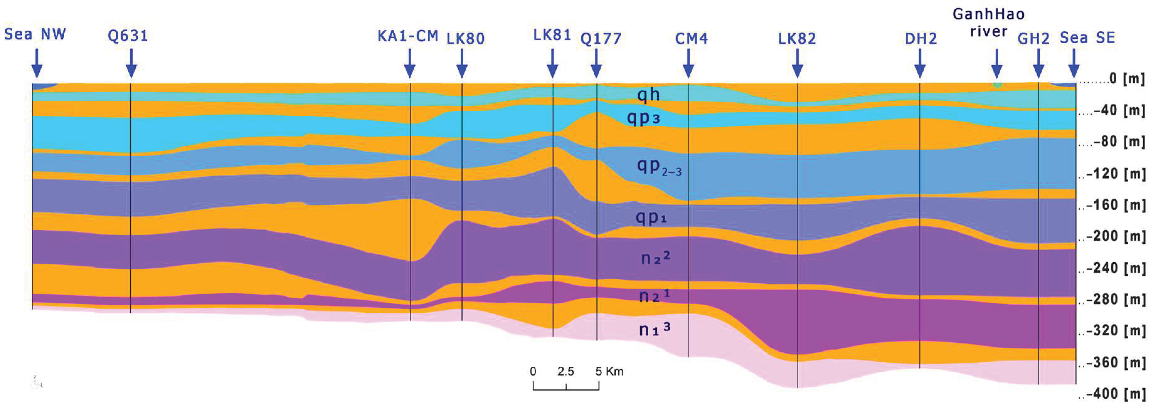
With an average topography of about 1 to 2 m (Hoan et al., 2022) above sea level, the CMP lies at a relatively low altitude above sea level. The costal line of the model area is about 396 km long. The ocean depth within a range of 30 km outside of the coastal line is about 60–80 m. The salinity of the ocean water is 35 g/L on average (Hung et al., 2019; Vengosh, 2013). The channel and river system of the CMP is highly influenced by tide. The inter-annual tide height is about 1–2 meters. This causes saline inflow into the channel and river system, with a maximum of nearly 33 g/L in the river system (Duong et al., 2016). The river system can be locally connected to the qh aquifer, as described by Duy et al. (2021). However, the surface water–groundwater interaction is limited in most areas, with the top aquitard having a thickness of several meters (Hoan et al., 2022, Figure 3 (cross-section)).
Geologically, there have been multiple transgression and regression periods, resulting in several-hundred-meters-thick sequences of marine and fluvial sediment deposits (Wagner et al., 2012). In recent geological history, the area is a consequence of the uplift of the Himalayan Mountains and the associated erosion. This eroded material was transported by the Mekong and deposited in its delta, forming the CMP. These deposits also exhibit a certain degree of salinity from former transgression/regression processes.
The surface water is interlaced by a large number of channels. These are used to transport people and goods, and to serve agricultural producers and fisheries. However, due to the tides, an exchange between salt- and freshwater, as well as between surface and the upper groundwater, is locally also possible, where the upper aquitard is shallow or not present at all. The conceptual model of the groundwater system of the CMP consists of seven aquifers (from top to bottom: Holocene–qh; upper Pleistocene–qp3; upper–middle Pleistocene–qp2–3; lower Pleistocene–qp1; middle Pliocene–n22; lower Pliocene–n21; and upper Miocene–n13; Figure 3). These aquifers are separated from each other by impermeable aquitards. However, the continuity of these aquitards has not yet been fully clarified, and is part of this evaluation.
Figure 3.
Hydrogeological structure of the Ca Mau Peninsula. Aquitards in orange color and Aquifers in color range from blue to magenta (modified after Hoan et al., 2022).
Figure 3.
Hydrogeological structure of the Ca Mau Peninsula. Aquitards in orange color and Aquifers in color range from blue to magenta (modified after Hoan et al., 2022).
The groundwater in the deep aquifers in the study region consists of brackish, saline, and fresh types. Previous studies revealed that the determination of groundwater age is inconclusive, ranging from recent to older than 45 ka, but with an increasing trend from Pleistocene to Miocene aquifers (Bauer et al., 2022; Hung et al., 2019). The saline water in the deep aquifers could result from the diffusion of saline pore water and/or salt intrusion into freshwater resources. Additionally, in the Mekong Delta, the hydraulic interaction between the surface rivers and channel system and the aquifer system does not reach down to qp2–3 (Doan et al., 2018). The interaction between deeper aquifers might be caused by natural conditions (thin aquitard layer, hydrogeological windows, and hydraulic gradients) or anthropogenic factors (number of production wells, leakage along the well structure, and underground construction) (Bauer et al., 2022).
As mentioned in Hoan et al. (2022), the most exploited aquifers are qp2–3 and n22, accounting for 63.7% (361,580 m³/day in 2019) and 29.7% (168,600 m³/day in 2019) of the total pumping in 2011. According to a survey conducted in 2019, people in Ca Mau mainly use groundwater for many daily purposes. However, only 25.4% respondents in the survey used groundwater for drinking purposes (Pham et al., 2023). The higher salinity in the qp2–3 aquifer is only one reason for the minor use of groundwater for drinking in this aquifer. In addition, high values were recorded for other water-quality-related parameters (Fe, Mg, etc.) (Bauer et al. 2022), leading to the reduced use of water from qp2–3 for drinking. This information on the use of the respective groundwater has to be taken into account for discussion. Therefore, this study focuses on qp2–3 and n22.
3. Data Collection
Data was collected from the national groundwater monitoring network (NAWAPI, 2023), and international research cooperation projects such as the ViWaT project (https://www.viwat.info/english/21.php (20 August 2023)) and the IGPVN (https://igpvn.vn/ (20 August 2023)) project from 2013 to 2022 (including Ca Mau, Kien Giang, Soc Trang, and Bac Lieu; see Figure 4).
Total dissolved solids (TDS) and electrical conductivity (EC) are mainly used as groundwater quality parameters in investigations focusing on salinity, especially in the coastal area of Vietnam. Two parameters, TDS and EC, are able to indicate salinization of water resources and they can be used to study the seawater intrusion into groundwater (El Moujabber et al., 2006).
In the field, EC is measured directly, while TDS is calculated. Through experimental calculations, the relationship between EC and TDS (Lloyd and Heathcote, 1985) can be written as follows:
where TDS is the total mineralization (mg/L), EC is the conductivity of water determined at 25 °C (µS/cm), and k is the conversion factor, which ranges from 0.5 to 1.0 in natural waters (McNeil and Cox, 2000).
The conversion factor k has not been uniformly applied in the Mekong Delta study area. For example, Trung (2015) chose a coefficient of 0.64, while a factor of 0.67 was used in Pechstein et al. (2018).
The EC depends on the activity of ions in the solution, which in turn depends on the chemical composition, ionic strength, and temperature. EC is not directly linear as the conductive mobility of ionic species is variable, e.g., it depends on size and charge, and colloidal suspensions also contribute to conductivity. For example, in high-salinity solutions, the dissolved ions form non-ionic complexes that do not contribute to EC, but rather to TDS (Day and Nightingale, 1984; McNeil and Cox, 2000). Manh and Steinel (2021) therefore chose a non-linear correlation based on the most reliable set of 179 data points consisting of both EC and TDS data from Ca Mau Province.
Bauer et al. (2022) determined the average conversion coefficient k = 0.81 by considering the relationship between EC and TDS of 190 groundwater samples analyzed in a laboratory. A technical report by Manh and Steinel (2021) used the coefficients of 0.5 and 0.8 to evaluate the sensitivity of the change in the saline intrusion boundary based on different conversion factors.
In addition, the collected field measurement data may use different types of devices or different factors, depending on experience, or the meter may automatically convert EC to TDS. To obtain accurate TDS results, samples should be taken to the laboratory for detailed ionic analysis.
According to the data collected from the national groundwater monitoring network, automatically recorded measurements from sensors, and laboratory results of water samples collected by NAWAPI, the difference in k was between 0.51 and 0.76. In conclusion, while TDS values may potentially show variations in terms of absolute values as a result of the aforementioned challenges, the trend nevertheless remains.
For the CMP, numerous single-point measurements for salinity are available (see Figure 4), provided by different organizations (NAWAPI, DWRPIS, BGR and KIT) in different aquifers, even though the aquifer has sometimes only been deduced on the basis of well depth, and hence may have been wrongly assigned. These values can be used to determine the saline areas and freshwater areas in the different aquifers. This is necessary for initializing the boundary conditions of the model. The measured time series of salinity are necessary for the validation of the transient run of the model. For the period from January 2011 to April 2022, 23 time series (right side of Table 1) are available, describing a salinity analysis of water samples in the lab two times per year. In addition, for the period from January 2020 to April 2022, 15 time series (left side of Table 1) of automatically measured EC from the national monitoring network are available. The conversion factor was calculated by comparing EC from the field with TDS analyzed from water samples in the laboratory. In eight cases, these factors were evaluated as being lower than 0.5 and greater than 0.81. In these cases, the factor was corrected to 0.5 and 0.81, depending on the evaluated minimum and maximum factors mentioned above.
Saline and freshwater areas can be distinguished using the interpolation method in space for the point measurements, as mentioned above. Alternatively, regionalizing methods can be used, as presented by Gunnink et al. (2021). The dataset, available on a 1 km by 1 km grid, incorporated groundwater points with TDS and wells with geophysical logging. An additional dataset for Ca Mau Province is that made available by Manh and Steinel (2021). To regionalize these data for each aquifer, a detailed data analysis and interpolation using the kriging method were carried out. The result was a homogenized saline dataset for each aquifer. Therefore, in principle, two homogenized datasets are available for the CMP.
Time series of the measured data from 2011 to 2023 did not show any significant trend in the lower aquifers regarding salinization (Manh and Steinel, 2021). In Figure 5a, the measured TDS data for the aquifer qh is presented. Only selected monitoring wells in aquifers qh and qp3 showed some trends, e.g., at Q177, Q199, and Q401 (Figure 5a). This trend may have been caused by surface penetration, dry and rainy seasons, tidal or artificial effects. No long-term increase in salinity in qh could be inferred from the available data on a regional scale.
The deeper monitoring wells exhibited stable salinity levels, with minor changes, except for a few wells that were monitored for two years, where the trend was unclear. In Figure 5b, the automated TDS monitoring data of groundwater wells in the ViWaT projects at two monitoring locations, GW1 and GW2, are visualized. The data showed that different levels of TDS were established at two sites in different aquifers over time. However, the observed change in TDS in the aquifers is not significant.
4. Methodology
4.1. Governing Equations
The three-dimensional mathematical solute transport model of hydrodynamic dispersion equation is as follows:
The salinity of water affects the density of the respective water. Therefore, to simulate the flow of groundwater in aquifers with variable salinity, it is necessary to convert the water level in the aquifers to the freshwater level using Equation of Ghyben and Herzberg (4.3):
where h, hf are saline and freshwater level (m); ρ, ρf are the densities of groundwater and seawater; and Z represents the height.
Conservative transport refers to the movement of inert substances dissolved in water. Solutes are affected by advection (the movement of the solute as linked to flowing water) and dispersion (dilution of contaminated water with clean water, which causes the size of the contaminated area to grow while reducing peak concentrations). To enhance a flow model to a transport model, additional parameters (e.g., porosity and dispersity) need to be specified (Figure 6), and initial and boundary conditions have to be determined.
The output of the transient transport model is the concentration at each node in the model domain during the considered time period. The calculated concentration values can be compared to observed concentrations as well as to qualitative information, e.g., the information that the salinity in the water of pumping wells is increasing.
4.2. Saline Intrusion Model Setup
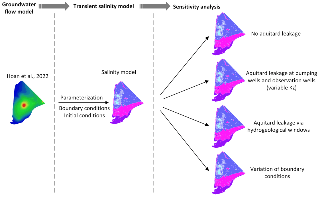
Figure 6 illustrates the process of enhancing the existing flow model of Hoan et al. (2022), making it a transient salinity transport model with a subsequent sensitivity analysis, which will be discussed later in more detail.
Figure 6.
Flowchart of the processing method.
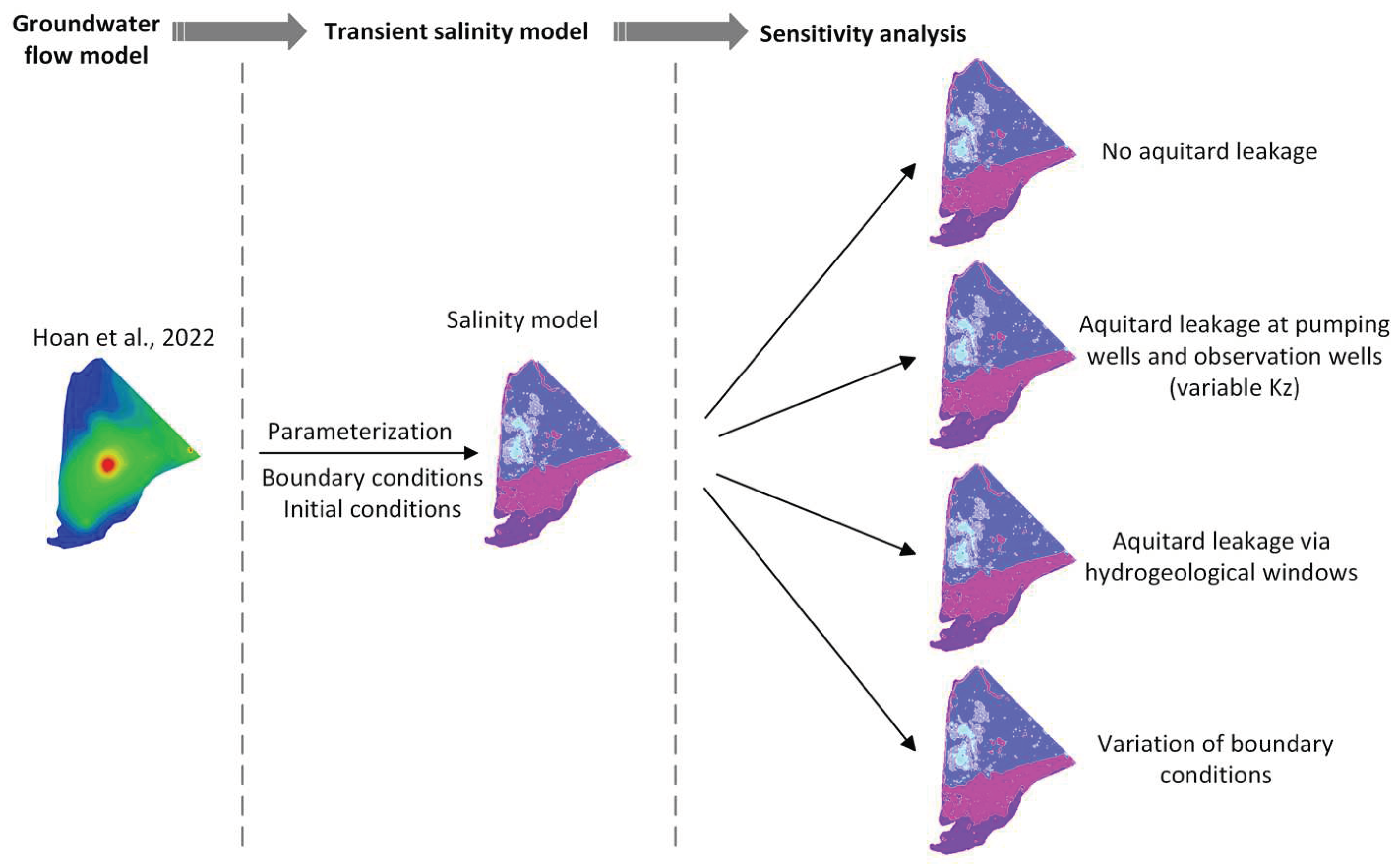
The density-dependent transient transport model for CMP was set up with the software FEFLOW for the time period from 2011 to 2022. The following salinization processes on the CMP were considered in the model:
- Infiltration from saline surface water sources (rivers, canals, aquaculture ponds, salt production, tidal inundations) into the upper aquifers identified by the land use map;
- Lateral saline intrusion from the offshore areas into the aquifer system induced by pumping, assuming freshwater/saline water in deep aquifers is extrapolated from inland data up to 30 km offshore;
- Salinization by mixing and dispersion from areas with higher salinity into areas with lower salinity along the flow path;
- Down or upward leakage from one aquifer to another through hydraulic windows in the aquitard either natural or from well drillings.
4.2.1. Groundwater flow Model
The groundwater flow model, which is used for the salinity model, was described in Hoan et al. (2022). The mass transport was activated in FEFLOW for the calculation of the salinity transport. Moreover, the finite element mesh was refined, both on a horizontal and vertical scale, in order to achieve a mesh size sufficient for simulating salinization processes, in particular around the pumping wells, where the hydraulic conductivity is locally changed.
4.2.2. Mass transport Model
For the mass transport model, TDS was used in our modeling to represent salinity. During the validation period, the observed TDS values from a total 14 well groups were used in the period 2011–2022.
4.2.2.1. Model Boundary Conditions
The following boundary conditions were considered:
- 1)
- Sea water intrusion implemented on the basis of Dirichlet boundary conditions with defined concentrations: for Layer 1–Layer 5, representing the aquifers qh and qp3, this was set as 35 g/L (similar to the current TDS of seawater), while for Layer 6–Layer 14 this was set as 3 g/L for the model boundary offshore;
- 2)
- No boundary conditions for salinity at the northern border;
- 3)
- Land-use-based estimation of human activities influencing the salinity in the qh aquifer. These activities were determined using land use maps (Stolpe, (2023), Figure 7, left side). For most land use classifications, a salinity value was fixed (see Figure 7, right side) for the initial conditions of the top layer depending on the predominant land use class in each region. At selected locations, the boundary conditions were applied as transient mass BCs with the dynamics illustrated in Figure 8 with monthly data.
- 4)
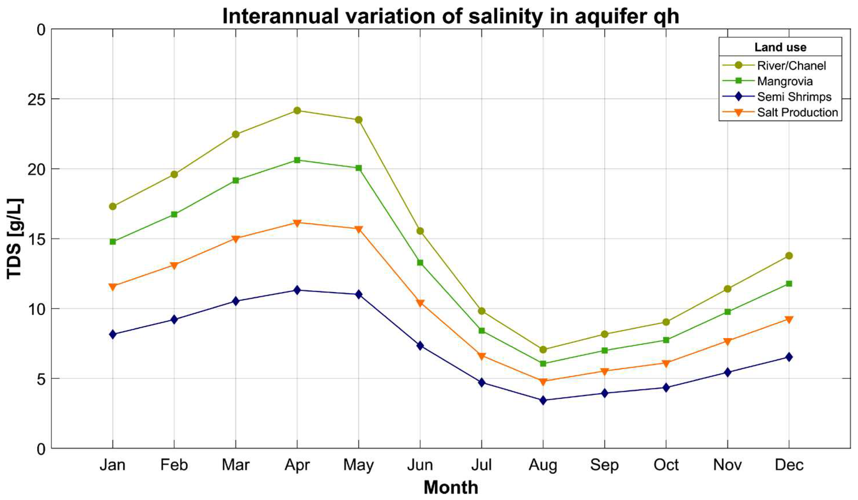
- Surface water–groundwater interaction: the channel and river system on the CMP is highly influenced by the tide system of the ocean. The water levels in the river and channel system were interpolated from measurements based on the mean monthly change in water level. In addition, we used measured mean monthly salinity data (Ca Mau and Song Doc stations) to interpolate interannual variation of the surface water bodies, mangrove, and semi-intensive shrimp and salt production (shown in Figure 8).
Figure 7.
Land-use-dependent salinity initialization (a) (based on Stolpe, (2023)) and TDS classification based on land use (b).
Figure 7.
Land-use-dependent salinity initialization (a) (based on Stolpe, (2023)) and TDS classification based on land use (b).
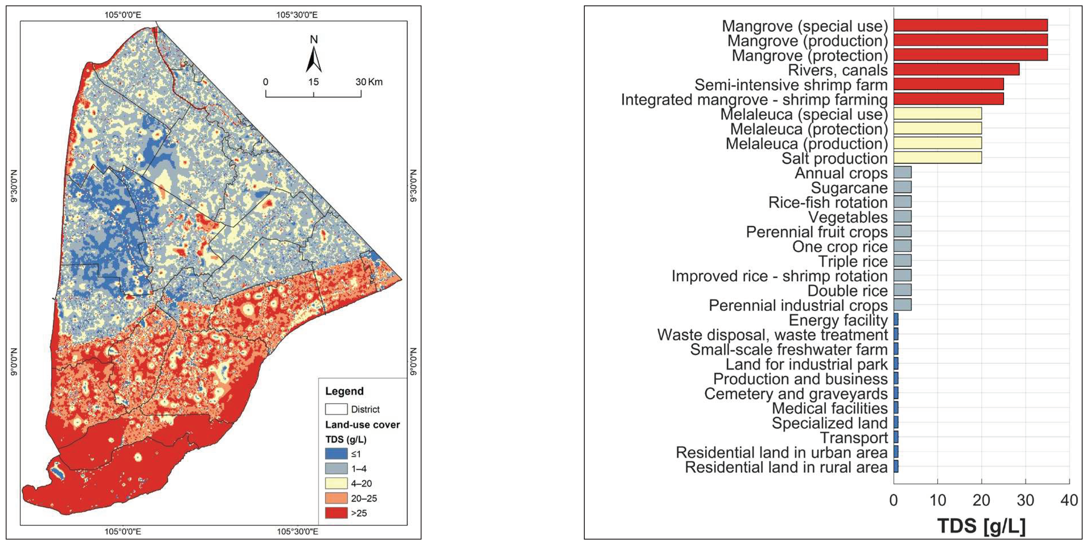
Figure 8.
Mean monthly salinity for different land use types applied for model boundary conditions in aquifer qh and the top layer (derived from salinity of surface water monitoring stations of Song Doc and Ca Mau, period 2012–2020).
Figure 8.
Mean monthly salinity for different land use types applied for model boundary conditions in aquifer qh and the top layer (derived from salinity of surface water monitoring stations of Song Doc and Ca Mau, period 2012–2020).
4.2.2.2. Initial Conditions
Initial conditions were estimated for the first-time step (Jan 2011) to initialize the model in space for all the aquifers. According to the reduced information of time-equal measurement of salinity data, all the available salinity data in space were used to prepare horizontal salinity.
A combined dataset was established from the regionalized data of the IGPVN project (Manh and Steinel, 2021) for the aquifers qp3, qp2–3, qp1, n22, and n21 inside Ca Mau Province and interpolated values outside of Ca Mau Province on the basis of values measured during our data collection.
One of the challenges was determining the initial TDS concentration for the upper layers. There are many lakes, ponds, and rivers/channels, covering about 60% of the study area. However, their common feature is that salinity changes with the season. Data on these changing salinity levels are not available.
Therefore, the salinity in Layer 1 and Layer 2 (qh) was determined according to the zoning of land use types combined with surveying some specific point groups. For the aquitards, the same initial conditions as in the upper aquifer were applied. Although some areas are controlled by sluice gates, salinity measurements in these areas vary within a relatively small range. Consequently, the TDS value is considered to be a time-constant boundary condition for areas, which are controlled by sluice gates. The initial conditions for all aquifers are illustrated in Figure 9. As for the remaining regions and land use types, their salinity variations were estimated through interpolation based on seasonal changes throughout the year (as depicted in Figure 8).
4.2.2.3. Density Flow Parameter Adaptation
Flow velocities and hydrodynamic dispersion coefficients are key parameters for the description of fluid and solute transport in porous media. The topic of dispersivity has interested many in the scientific community, including those studying hydrology and contaminants, and for some time now, flow through porous media has been investigated (e.g., Grathwohl (1998); Jacques W. Delleur (2019); Sahimi (1981); Bear and Verruijt (1987); Koch and Brady (1987)). Hydrodynamic dispersion includes both mechanical (convective) dispersion and molecular diffusion. For low fluid velocities, solute dispersion is determined by molecular diffusion; for high values of velocity, convection becomes dominant, but the contribution of diffusion cannot be neglected.
The following dependencies of dispersion from the soil and sediment are known from literature:
1. The dispersivity coefficient for homogeneous soil and layered heterogeneous sediments show that stratification affects the dispersivity coefficient, and the dispersivity coefficients for layered heterogeneous sediments are nearly two times lower than those in homogeneous sediments. (Leij and Van Genuchten (1995), Al-Tabbaa et al. (2000), Zhang and Wu (2016), and Sternberg (2004)).
2. The dispersion coefficient is influenced by the distance of travel, and its values undergo changes as distance increases. In both homogeneous and layered heterogeneous sediments, the dispersion coefficient values increase by a factor of 2.5 with the expansion of horizontal travel distance. ( Gelhar et al. (1992), Khan and Jury (1990), and Sudicky and Cherry (1979)).
3. There is also a dependence of the dispersion coefficient on the sediment type. From sand to clay, the dispersion coefficient decreases with smaller diameter of the material.
Therefore, in this study, the Waterloo Hydrogeological Database (Nilson Guiger and Monalisa Horvath 2003) was used to calculate the average longitudinal dispersivity coefficients and flow distances for different sediment types in the multilayered aquifer system of CMP. These coefficients were normalized by the flow distance (Figure 10a) and multiplied by the averaged element diameter of the finite element mesh of the model (ca. 50 m; Figure 10b). According to point 1, we assumed that sediments are homogeneous within the sediment classes presented in Figure 10, because detailed information about the sediment structure is not available. Thus, the value was multiplied by a factor 2.5. The regional distributions for the sediment type-based coefficients for the aquifers qp2–3, qp1, n22, and n21 are shown in Figure 10c–f.
For Vietnam’s aquifers, different papers or reports exist dealing with the estimation of dispersivity coefficients. Thanh et al. (2017) described a groundwater fieldwork pumping and tracer injection test in Nghiem Xuyen commune, Thuong Tin district, Hanoi, where a salinized and fresh groundwater boundary exists in the Pleistocene aquifer. The tracer experiment was conducted during a 60 h pumping test. The result was a longitudinal dispersivity value of 2.5 m, with an effective porosity of 0.32. In four other reports ( DWRPIS, 2021a; DWRPIS, 2021b; DWRPIS, 2021c; DWRPIS, 2021d), the results of different pumping tests in the Mekong Delta were determined (Table 2). In the process of these pumping tests, when the water level reached the steady state (after 48–72 h), salt was injected into the observation well until 150 kg of salt was dissolved, and the total time for each experiment averaged more than 20 days. These dispersivity coefficient results differ significantly from each other (0.02 – 2.5) due to the many influencing factors, such as the constant pump rate throughout the pumping test, the pumping well not being cleaned before the experiment, the salt injection process, and asynchronous machinery. In addition, there are natural factors such as the heterogeneous nature of the sediment types and the thickness of the aquifer.
The longitudinal dispersivity coefficient varied between 0.02 m and 2.5 m, with an effective porosity of between 11.5% and 32%. Thus, the abovementioned dispersion coefficients are in the range of the used sediment-based coefficient without the layer-based factor (blue columns in Figure 10b), thus representing the best method that could be achieved.
4.3. Limitations of the Model
In order to evaluate the groundwater salinization processes in the Mekong Delta, the model was adapted accordingly with the given dataset. However, the model possesses some limitations due to the limitations of the available data.
No private household wells are included in the model, since household wells operate with very small flows. Instead, for the model the water consumption for each commune is derived based on the population and an average rural water demand of 34 L/person/ day (Hoan et al., 2022). This water consumption for each commune is implemented in the model by several wells with a total flow rate equivalent to the derived water demand. By this method, the assumed amount of water extraction by a large number of private household wells is represented by fewer wells in the model.
The drilling time of wells is not considered during the transient model calculation: all wells are in the model throughout the whole calculation period. However, in reality, many of the deeper wells were drilled later than shallow wells. This time dependency could be respected in further evaluations.
5. Results
5.1. Model Salinity Calibration and Validation
The groundwater flow model validation was discussed in detail in Hoan et al. (2022). According to the described validation criteria, salinity modeling can be performed for the purposes of confidence building and scientific validation. As stated by Davis and Goodrich (1990), confidence building “is a measure of the adequacy of the model structure (conceptual model and mathematical model) in describing the system behavior”, and salinity modeling “is a measure of the accuracy of the model input parameters relative to experimental results and field observations”. For validation in space, the scientific view postulated by Jackson et al. (1992) demands the validation of specific models “that one might reasonably expect someone with relevant technical knowledge to consider the model acceptable”.
The quality of the model was tested with respect to space and time for different aquifers according to Davis and Goodrich’s (1990) second point mentioned above. In Figure 11, the monthly measured and calculated salinity values for different levels are shown as a time series. The upper aquifers qh from Q199010 (Figure 11a), Q17701T (Figure 11b), and Q597020M1 (Figure 11c) featured the measured and calculated values with the best fits in the model.
Aquifers qh and qp3 showed that the fluctuation of the water level tended to be stable, but the model did simulate the seasonal effect of salinity. The salinity in the deeper aquifers qp1 and n22 tended to be stable, without interannual variation. Figure 11 (a, b, c, d) shows that the simulated (Q199, Q188, Q177, Q597, and 608) salinity levels could capture the salinity groundwater system behavior over a long-term validation period in the complicated exploitation setting.
Figure 11.
Time-dependent comparison of measured and modeled salinity for different well groups and aquifers.
Figure 11.
Time-dependent comparison of measured and modeled salinity for different well groups and aquifers.
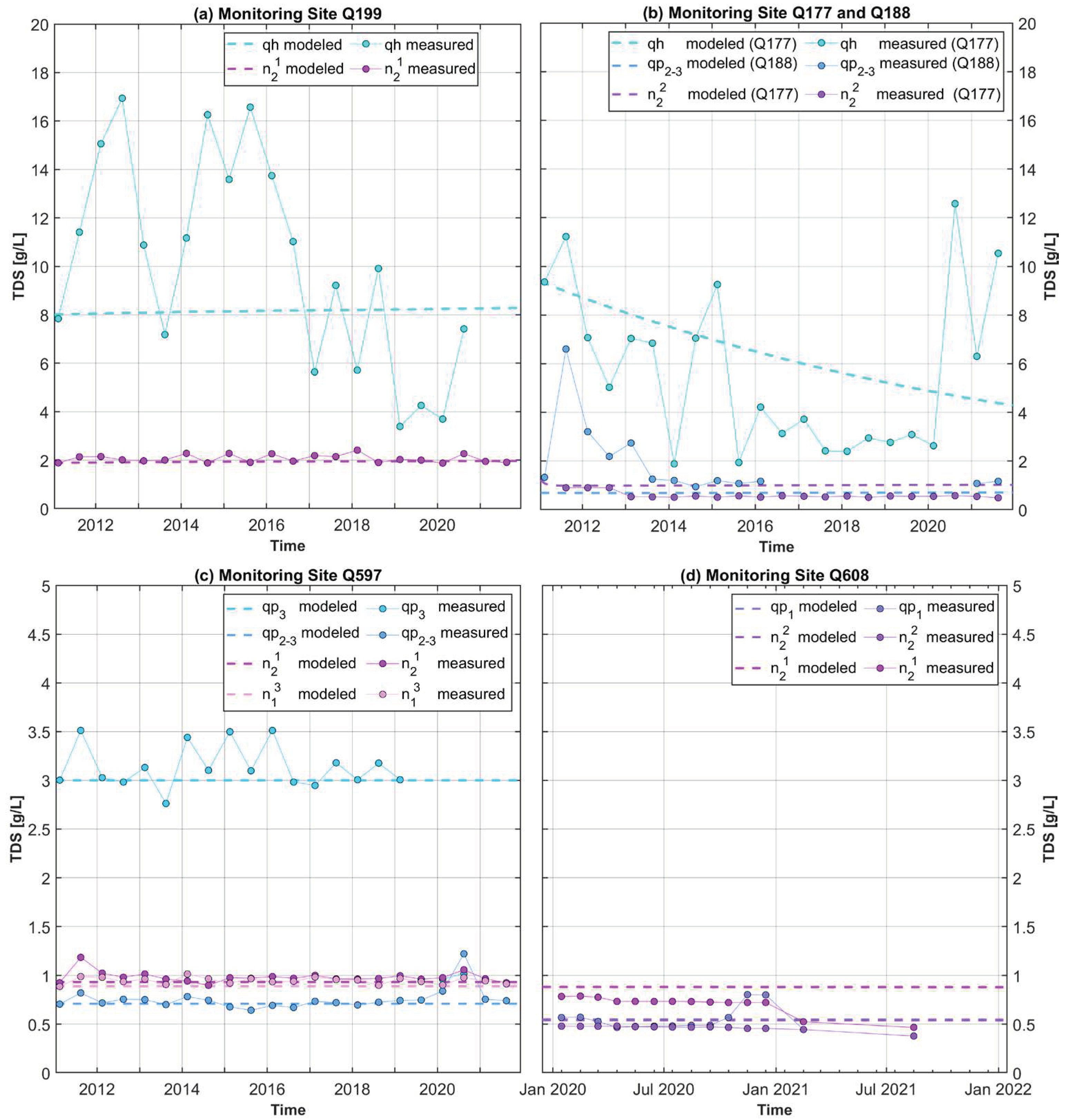
Figure 11 shows that at the presented monitoring wells the modeled TDS concentrations fit the observed values quite well in terms of magnitude and temporal evolution. The rather stable trend of observed TDS concentrations is met well by the model. Interannual variations in the observed TDS concentrations were not mimicked by the model, even though as described above, at selected locations interannual variations of TDS boundary conditions in qh were applied. At site Q199, the observed variations of TDS concentrations were not met by model, indicating that a refined consideration of locations with interannual variations of TDS boundary conditions in qh could improve the model results, as at Q199 site, constant TDS boundary conditions were applied.
The spatial salinity distribution is mainly influenced by the initial conditions and boundary conditions. Therefore, depending on the dispersion coefficient, the development of the salinity was simulated in the different aquifers. The calculation of salinity intrusion from the surface depending on land use classification led to a more detailed salinity distribution in the aquifers qh and qp3.
Figure 12.
Modelled salinity in aquifers qh and qp3.
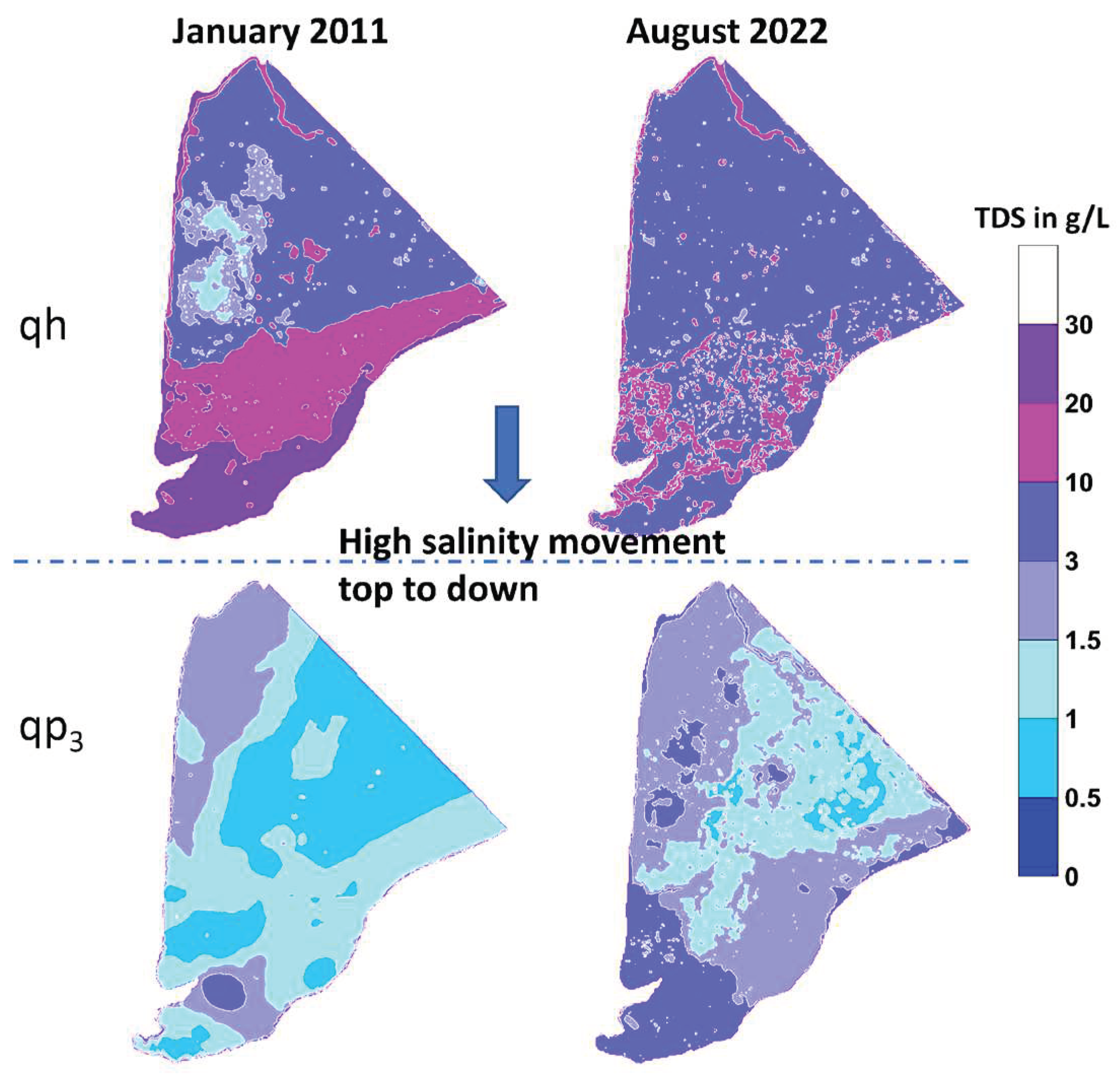
The salinity distribution in January 2011 was defined as the initial conditions in aquifers qh and qp3 (see Section 4.2.2.2). In August 2022, there was an increase in salinity in the aquifer qp3 (Figure 12, bottom middle), caused by a high transport from qh to qp3. Through the long-term simulation, we found additional salinity import from the top (Figure 12, top right) and ongoing salinity transport from the top down (Figure 12, bottom right). Because no space-dependent distributions of salinity for different times were available, the results of the salinity distributions for different aquifers could not be validated in detail.
As a common result for the criteria as described in detail in Section 4.2.2, the system behavior for salinization is considered to be well represented in the model from a confidence-building view because the calculated salinity was validated against point-measured salinity data (Figure 11) and the simulated results agree fairly well in terms of magnitude and temporal evolution. This is also in agreement with the second criteria for the operational view of model validation, i.e., “that a good, correct, or sufficient representation of reality” in time and space (Figure 12 and Figure 13) can be achieved with the model. Moreover, the model can be considered to be acceptable, as the knowledge of the hydrogeological and salinity context in the CMP was used for the model setup.
Figure 12 shows that the salinity transport was dominated by input from the surface, the modeled salinity in the two upper aquifers qh and qp3 show a strong change over the simulation period. In contrast, the lower aquifers qp2–3 and n22 show less changes in salinity over time (comparison of two lower maps in Figure 13 (a, b, d, e)). The scale is defined within an interval of 1.0 g/L. For the deeper aquifers qp2–3 and n22 (Figure 13a, b, d, e), no significant lateral change in salinity change can obtained from the model results during the simulation period. The Figure 13 (a, b, d, e) looks for both aquifers very similar. In the current model stage, only a small-scale variation in salinity due to pumping can be detected. However, this is consistent with the time series measurement of salinity, as no significant changes in salinity over time could be observed (see Figure 11). Figure 13 (c, f) show the modeled spatial changes of freshwater zones (< 1g/L) between 2011 to 2022. For both evaluated time steps, the 1 g/L isolines are shown. In figure 13c for qp2–3, two regions are marked: region 1 shows an increase of salinity along the border originated salinity inflow from the ocean, region 2 has increased salinity extending from the northern boundary (Bac Lieu Province) as a result of extensive groundwater extraction, which in turn contributes to heightened salinity levels in the northern border area. There are some regions (regions 3, 4), where salinity levels exceed 1 g/L due to the horizontal movement of areas with higher salinity, rendering the water unsuitable for drinking. The change of freshwater for aquifer n22 (Figure 13f) is smaller than qp2–3 aquifer. In the East (region 5, 6) the salinity is increasing originated by slow lateral transport of salinity. In the southern part of the Ca Mau Peninsula, we additionally observed vertical salinity transport in the model from qp3 to qp2–3, this salinity originates from the mangrove regions from the upper layers (Figure 9). As the result of the model, we only observe small influences on vertical salinity movement in qp2–3 and n22, which result from pumping. Exploitation is simulated based on area-wide values rather than specific points. In regions with high pumping rates, such as Ca Mau city, the results therefore suggest stable salinity as compared to other regions, as illustrated in Figure 13 (d, e).
Figure 13.
Development of the salinity from 2011 up to 2022 for aquifer qp2–3 and n22.
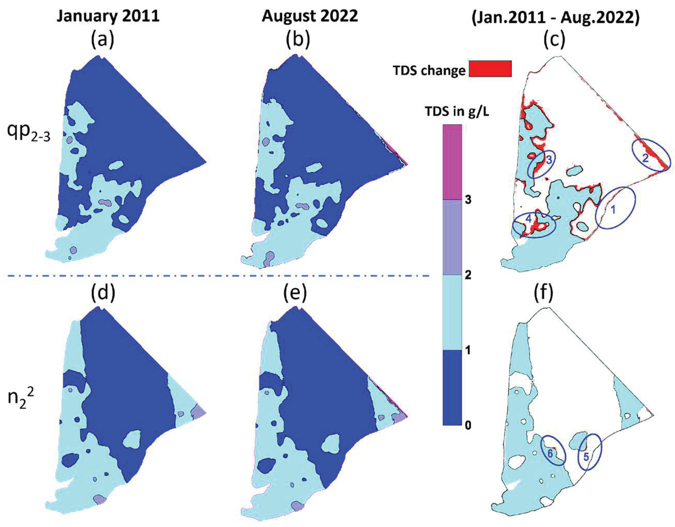
According to Pham et al. (2023), the study shows that among 144 questionnaires in Ca Mau, the percentage of exploited water allocated for drinking purposes was only 25.4%. Cooking accounted for 65.7% of the water usage, while 97% respondents use groundwater for washing activities. These freshwater areas are depicted as dark-blue regions in (Figure 13a, b) North-east Ca Mau Province. In the future, the number of areas with higher salinity is likely to increase due to similar pumping induced effects as illustrated in Figure 13c. Thus, this possibility of pumping freshwater from qp2–3 will decrease. In this area, freshwater has to be substituted from other sources, e.g., harvesting of rainwater or water diversion structures from other places. In regions with brackish groundwater, with salinity exceeding 1 g/L but below 3 g/L, it will be possible to use water in the qp2–3 aquifer for cleaning and washing in the near future.
5.2. Sensitivity Analysis for different levels of vertical hydraulic conductivity and initial conditions
To evaluate the possibility of local saltwater intrusion from the top to down at well locations, we assume a change in vertical hydraulic conductivity (Kz) due to the disturbance of the sediments around the wells caused by the drilling process in all aquitard layers above the tapped aquifer.
To avoid an overestimation of this process due to numeric effects, the aquitard layer beneath the aquifer qh was discretized into three layers. This refinement led to a regeneration of the model's mesh, culminating in a more intricate mesh comprising 11,397,424 mesh elements and 6,060,194 mesh nodes. Pertinently, key hydraulic boundary conditions (BC) including parameters such as pump rates and hydraulic head BC at the northern boundary, remained unaltered to ensure consistency.
Five possible scenarios are identified, as follows:
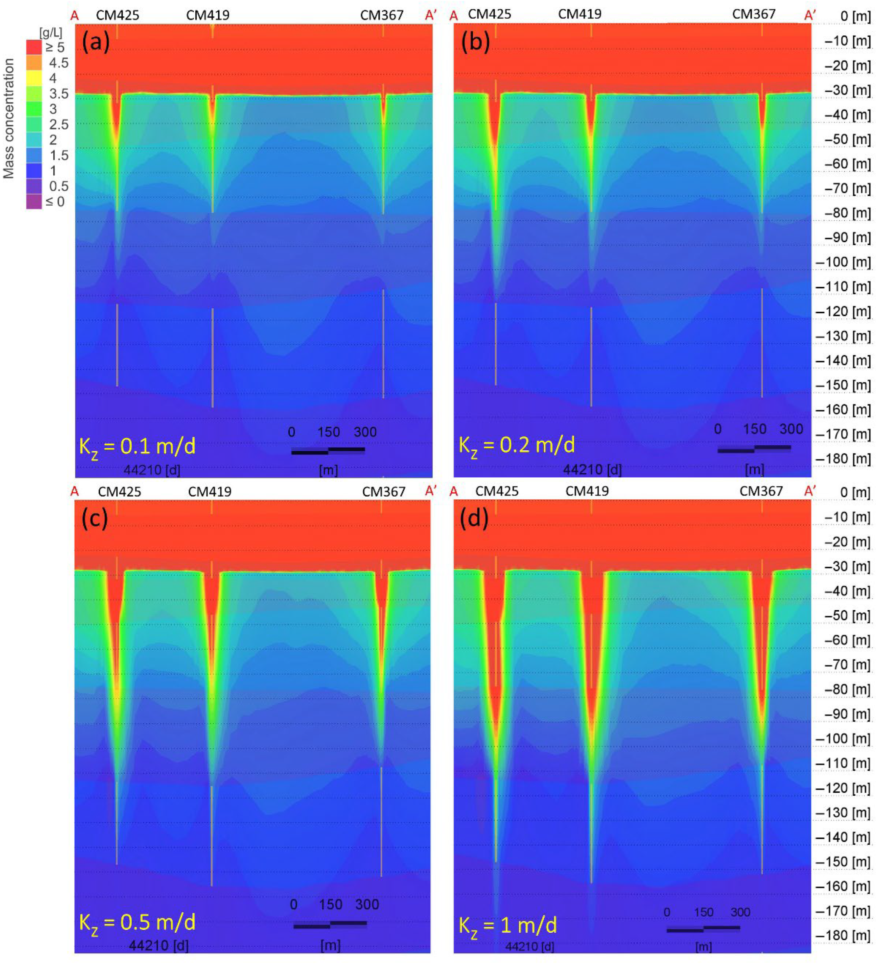
1) Scenario 1–4: Change of Kz at the production wells for the aquifers from unadapted to 0.1, 0.2, 0.5 to 1 m/d.
2) Scenario 5: There exists a hydrogeological window close to the production well with Kz = 0.1m/d.
The results of the sensitivity analysis show that such local disturbances of the sealing clay layers can enhance vertical salinization (Figure 14) processes as illustrated in an exemplary cross-section (Figure 3). We found that within a decade, the rate of vertical salinity intrusion will experience a significant boost, stretching from a depth of 30 m to a depth of 90 m. This phenomenon is in alignment with adapted Kz values ranging between 0.1 to 1 m/d in the aquitards (marked in orange color in Figure 14a–d). Conversely, when Kz is maintained at 0.1 m/d, the process of saline intrusion occurs at a slower pace, with the saline infiltrating to a depth of 55–60m within the same 10-year span.
Concerning the salinity of the extracted water, this temporal effect is crucial, as the high salinity concentrations (> 5 g/L TDS) did not propagate downwards to the pumped aquifer (below 155 m at CM425), hinting that for deeper aquifers, this effect is considered to increase, if longer time scales are considered.
Figure 14.
Kz simulation results on the cross-section AA’(a, b, c, d) and BB’(e) in 10 years, from 01.2011 to 01. 2021.
Figure 14.
Kz simulation results on the cross-section AA’(a, b, c, d) and BB’(e) in 10 years, from 01.2011 to 01. 2021.
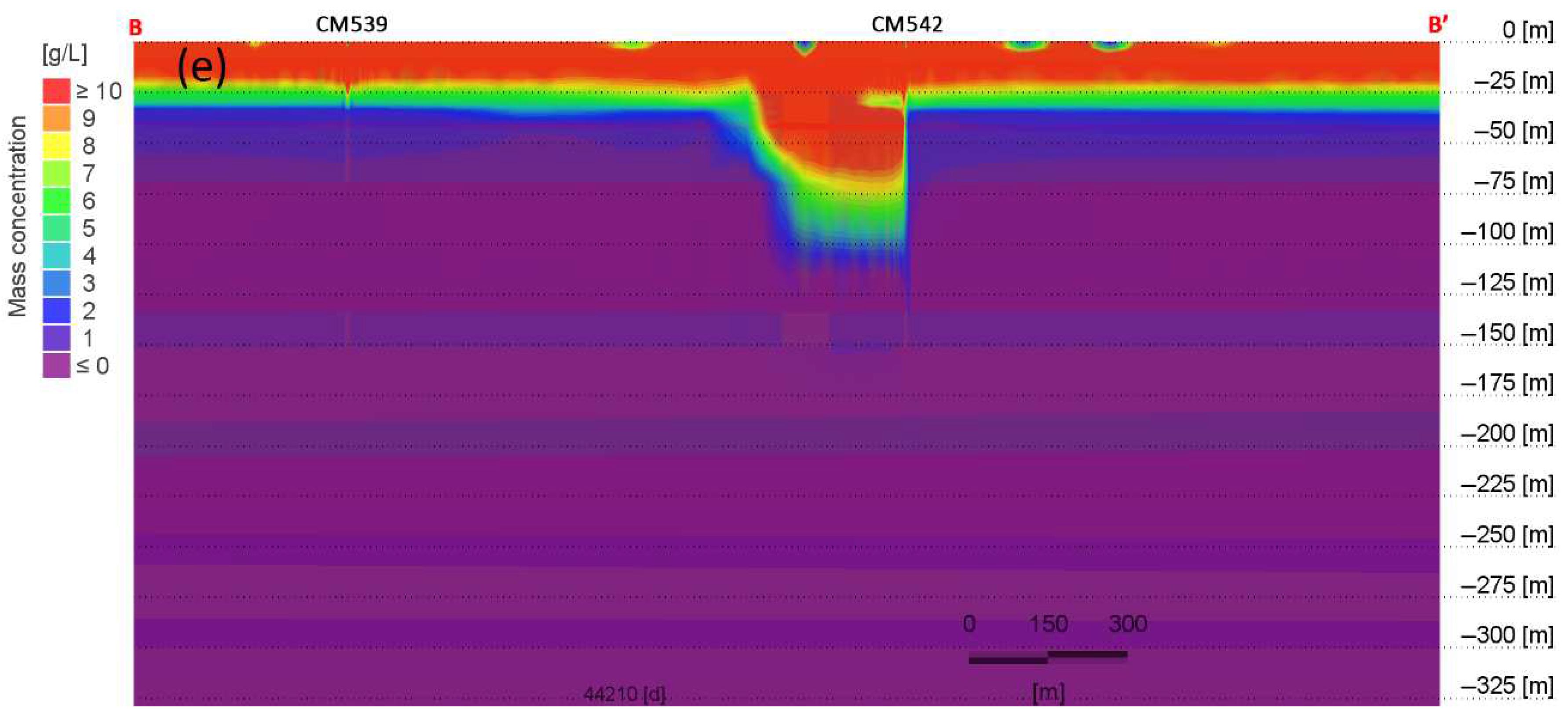
In addition, in one scenario a hydrogeological window (Figure 2) located near a production well (CM542, 720 m3/d) in a shallow aquifer (qp3) was implemented into the model. The results indicate that saltwater movement occurs at a considerable velocity from the upper layers, through the hydrogeological window, and flowing into the production well (Figure 14e). Depending on the pumping rate and the location of the hydrogeological window, the saltwater intrusion can occur quickly or slowly, or saltwater intrusion can occur due to gravity and diffusion or dispersion, if there are no pumping well nearby.
On the basis of personal communication during field research, we recognized a significant shift in the water extraction depth of many household wells over a span of seven to ten years. Instead of relying on shallow aquifers, households have transitioned to extracting water from deeper aquifers. This change can be attributed to the increasing salinity in the qp3 aquifer, where the concentration of TDS exceeds 3 g/L. Consequently, the drilling depth was extended to the adjacent qp2–3 aquifer. The findings are illustrated in Figure 14, which includes the qp3 and qp2–3 aquifers. In Figure 14a, b, the graphs depict the intersection between < 3 g/L (blue) and > 3 g/L (green) close to the aquifer between qp3 and qp2-3. In Figure 14c, d, this intersection is much deeper.
6. Discussion
The interaction between surface salinity and the upper aquifer qh in the MKD remains poorly understood. Elevate salinity levels in both soils and water bodies is a ubiquitous problem on the CMP. Salinity varies at the local scale (5–10 m), but the relative effects of land use and surface geology on salinity variation in the near-surface zone (<5 m) is unknown. Rahman et al. (2018) identified that “the influence of surface water salinity (associated with different land uses) on the groundwater salinity regime is pervasive”. They found that areas underlying the shrimp farm/tidal flat contained higher salinities irrespective of the near-surface sediment characteristics, while areas underlying the drinking water ponds or inhabited areas had relatively low salinity. In our model, the impact of land use and infiltration of surface water from the top into the qh aquifer was implemented to model the relation between land use and groundwater salinity.
Interannual variations of TDS concentrations at observation wells are most evident for the qh aquifer. But even in deep aquifers (e.g., in n21 at Q199 (Figure 11a) such interannual variations are observed. In order to model these dynamics, interannually variable TDS boundary conditions were applied at selected locations in the model for the qh aquifer. However, these dynamics in TDS concentration do not propagate to lower aquifers in the model. A lateral spread of these dynamics in qh from the selected areas with interannually variable TDS boundary conditions (such as river, channels) is limited by the constant TDS boundary conditions at other model nodes. For future studies, the location and variability of TDS boundary conditions in qh aquifer can be optimized in order to model the interannual variability of TDS concentrations in the deeper aquifers
Rahman et al. (2018) also described that the “distance from the river can also be seen as a factor; however, in reality, a more likely factor is the presence of saline water in the river compared to the other areas”. We found that the interannual salinity of Q199010 in aquifer qh varies between 6 and 10 g/L (Figure 9, top left). The distance of this observation well to the nearest river, which is strongly influenced by the tidal system and the rainy and dry periods, is about 100 m. Rahman et al. (2018) identified a distance from rivers of about 400–500 m as having an impact in this regard (4100–5500 μS/cm estimated for factor EC to TDS with k = 0.7, i.e., 2.8–3.8 g/L), which is in line with our results.
NAWAPI (2021) calculated salinity forecasts up to 2026, focusing on a 1.5 g/L shift in the saline boundary line in two different regions (below 1.5 g/L and above 1.5 g/L), they did not focus on the different salinity distributions in space. The work described in this article, presents a salinity distribution with improved detail. Due to the initialization dataset used for each aquifer, for a more accurate salinity forecast model could be developed. Our model indicates that the salinity movement in the deeper aquifers was seemingly slow, as predicted by NAWAPI (2021).
As neither the observed TDS concentrations in monitoring wells nor the modeled concentrations showed a significant increase in salinity during the simulation period from 2011-2021, further potential pathways of groundwater salinization were evaluated with the model by sensitivity analysis of the vertical interaction between the aquifers.
As illustrated in the cross section in Figure 3, the aquitard thicknesses vary a lot in the southernmost region of the Mekong Delta. This variation in thickness and the rather little number of available drilling logs upon the layer interpolation is based on, can be considered as indicators, that hydrogeological windows may indeed exist in different aquitards, even though they have not yet been identified in drilling logs. The integration of such a hydrogeological window nearby an extraction well in the model showed that vertical groundwater salinization can strongly be enhanced by such hydrogeological windows.
As a second pathway of potential vertical groundwater salinization, leakage at well locations was evaluated in a sensitivity analysis of the model, where disruptions of the sealing clay aquitards could cause vertical migration of saline waters into freshwater aquifers with more freshwater. This was implemented by a local increase of the hydraulic conductivity in z-direction (Kz) in 5 m around each well. The sensitivity of the model to different Kz adaptions was subsequently evaluated (Figure 15).
Figure 15a shows the temporal and spatial average modeled salinity in observation wells and pumping wells under different Kz scenarios for the aquifers qp3, qp2-3, qp1 and n22. For the simulated TDS concentrations of the lower aquifers qp1 and n22 (squares and diamonds in Figure 15a), there is neither a significant difference between the observation wells and pumping wells, nor can an effect of the variation of Kz be inferred from the sensitivity analysis. In contrast, for the wells in qp2-3 (circles in Figure 15a) an increase in salinity with increasing Kz can be concluded from the modeled data. Additionally, TDS increases nearly equally for both the observation wells and pumping wells in all tested scenarios.
In the uppermost considered aquifer qp3 (triangles in Figure 15a), TDS shows a significantly higher increase in pumping wells than in observation wells, indicating that pumping activates might enhance such vertical salinization pathways.
In lower aquifers, this effect is likely to be damped due to mixing processes and is considered to be delayed, so effects might occur later than the modeled period of 10 years.
As the effect of vertical salinization due to a disruption of clay layers during the drilling process is strongest in qp3, a more detailed analysis of the modeled data is presented in Figure 15b. The graph shows for each simulated timestep between 2011 and 2021 the statistical distribution of modeled concentrations as overlapping boxplots with the average concentrations as black lines, the 25–75 percentiles in the color codes for each scenario and the box plot whiskers in light grey color (outliers were not plotted).
The results indicate that an adaption of Kz to 0.1 m/d leads to an average increase from 2.0 g/L to 5.5 g/L for observation wells and 2.4 g/L to 4.6 g/L for pumping wells, respectively, over the simulation time. By contrast TDS concentrations in the scenario with unadapted Kz, increase only from 1.9 g/L to 2.7 g/L in observation wells and 2.3 g/L to 2.7 g/L in pumping wells during the simulation period. The increase of TDS is mainly characterized by an initial rise during the first year of simulation and a rather stagnant trend thereafter. The stronger increase in observation wells compared to pumping wells might be due to the relatively small numbers of available observation wells in qp3.
The salinization dynamics however change particularly for the pumping wells with increasing Kz -adaption, which can be derived from the continuously rising average concentrations in the pumping wells for Kz = 0.5 m/d and Kz = 1.0 m/d, reaching an average salinity of 8.2 g/L and 9.7 g/L, respectively, while in observation wells the concentrations remain after an initial rise at 5.8 g/L and 5.5 g/L, respectively.
This demonstrates that if the aquitards are locally disrupted by the drilling process of a well in an order of magnitude, the salinization process is much faster in a regularly pumped well compared to an observation well without regular pumping. This effect could explain the differences in stable TDS concentrations across different well types and the need of farmers to drill deeper wells, as the water of their previous wells became more saline over time. It is worth noting that even Kz values of > 1.0 m/d could be possible due to the backfalling of sandy aquifer sediments into the well anulus after drilling, leading to even higher and faster salinization effects. This study is the first study to quantify such potential processes for the Mekong Delta.
Furthermore, to assess whether seawater intrusion affects the groundwater salinity of inland areas, two model runs were carried out, (1) with boundary conditions from layer 3 to layer 17 with a salinity boundary condition of 35 g/L at the offshore model boundary approximately 30 km away from the coastline and (2) without any offshore salinity boundary conditions. The comparison of both simulation results over a period of ten years indicate that the entire inland region remains unaffected by saline intrusion from the offshore boundaries. The mass flow rate [g/d] over a cross section along the coastline differed less than 0.1% between both scenarios. This underlines, that the choice of offshore boundary conditions for such short simulation times of 10 years, due to the slow groundwater flow velocities, has much less impact on the salinity dynamics than the choice of initial conditions, land-used based top-boundary conditions and the hydraulic conductivity of the sealing layers in the vicinity of the wells.
Thus, the results of this study demonstrate that the management of pumping wells and the well construction process can potentially have a significant impact on salinization processes in the aquifers. Moreover, this first evaluation of potential impacts of vertical salinization due to a disruption of clay layers during drilling process can help to understand the discrepancy between rather stagnant salinities measured in observation wells and the reported increasing salinity of private household wells. This also could indicate that the salinization of the aquifers is not necessarily a regional phenomenon, but partly a local issue.
Further investigations in the comparison between TDS concentration of monitoring wells, active extraction wells and abandoned extraction wells is necessary to better understand the impact of pumping and well construction to local groundwater salinity.
7. Conclusions
A new groundwater model, built upon previous work by Hoan et al. (2022), was introduced in order to enhance the understanding of saltwater dynamics and salinization processes on the CMP. Therefore, the 3D transient groundwater flow model was enhanced to a density dependent transport model for salinity.
A new method for determining transport relevant parameters, such as dispersivity as a function of sediment type, was applied. In addition, the land-use-based interannual salinity impact from the top to the qh aquifer was included, as well as infiltration from the river system and from mangrove areas.
These new aspects led to the detailed identification of high-salinity regions in aquifer qh, which also influenced the dynamics of salinity in qp3 and in parts of qp2–3. In the deeper aquifers, most of the water was freshwater (TDS below 1.5 g/L). Only in the NE Ca Mau (Bac Lieu) were there regions identified as possessing higher salinity.
The conservative mass transport model was validated against time period of salinity measurements in observation wells in different aquifers. The results showed a good agreement between the salinity based on measurements and the simulated salinity.
The sensitivity analysis of the hydraulic conductivity of the sealing aquitards around the wells indicated a potentially significant influence of the drilling process and the uncontrolled refilling of the borehole annulus. This could be demonstrated by the substantial amount of saline water leakage along casings of the pumping wells under for different Kz scenario. These processes could play a crucial role in the intrusion of saline water into the deeper aquifers and might even increase in the future. Also, the implementation of hydrogeological windows into the aquitards in the model showed a substantial amount of saline water leakage downwards.
Due to the limited coverage of the monitoring network, it is crucial to develop a groundwater management approach that addresses not only horizontal but also vertical salinity intrusion. This requires measures to prevent vertical saltwater intrusion into the aquifer. Some of these measures should include repairing damaged groundwater wells, preventing their usage, and restricting the exploitation of areas adjacent to hydrogeological windows above or below the saline aquifers.
Moreover, a broader monitoring effort, including active and abandoned pumping wells, should be set up to further investigate the proposed concept.
For further forecasting scenarios, the impact of existing active and abandoned extraction wells should not be disregarded.
However, these results and suggestions are only applicable to the issue of groundwater salinization. Overexploitation can also lead to significant land subsidence, which was not discussed here.
In conclusion, groundwater resource managers need to investigate coastal saltwater sources in detail, develop an early warning system for depletion and saltwater intrusion, protect zones, reduce groundwater exploitation, manage and supervise the construction of pumping wells, and fill damaged wells, while exploring alternative groundwater sources such as artificial groundwater recharge, rainwater harvesting, surface water, and water transport from other areas. Furthermore, the consequences of overexploitation in terms of land subsidence should be considered when planning the future of CMP.
Author Contributions
Conceptualization, Tran Viet Hoan, Stefan Norra, Karl-Gerd Richter and Felix Dörr; methodology, Tran Viet Hoan, Karl-Gerd Richter, Felix Dörr and Jonas Bauer; software, DHI WASY; validation, formal analysis, and investigation, Tran Viet Hoan and Karl-Gerd Richter; resources, Le Thi Mai Van, Anke Steinel, Nicolas Börsig and Stefan Norra; writing–original draft preparation, Tran Viet Hoan and Karl-Gerd Richter; writing–review and editing, Tran Viet Hoan, Felix Dörr, Karl-Gerd Richter, Jonas Bauer, Nicolas Börsig, Anke Steinel, Le Thi Mai Van, Pham Cam Van and Stefan Norra; supervision, Stefan Norra; funding acquisition, Stefan Norra. All authors read and agreed to the published version of the manuscript.
Funding
This study was funded by the Karlsruhe Institute of Technology, German Ministry of Education and Research (BMBF), the ViWaT Engineering research project, and the Catholic Academic Exchange Service (KAAD).
Institutional Review Board Statement
Not applicable.
Informed Consent Statement
Not applicable.
Data Availability Statement
The data provided in this paper are available upon request to the corresponding author. A permission letter (18 March 2022) was obtained from NAWAPI for collecting the rainfall data, groundwater quality data, surface- and groundwater-level data, and water exploitation data.
Acknowledgments
This paper benefitted substantially from the comments and suggestions of the two anonymous reviewers. The KIT-Publication Fund of the Karlsruhe Institute of Technology, the German Ministry of Education and Research (BMBF), the Research ViWaT Engineering project, the Ministry of Science and Technology (MOST), and the Catholic Academic Exchange Service (KAAD) supported the work described in this publication. This work was a contribution to the catchment Mekong project of Vietnam (VIWAT-Mekong http://www.viwat.info/english/21.php).
Conflicts of Interest
The authors declare no conflicts of interest.
References
- Al-Tabbaa, A., Ayotamuno, J. M., & Martin, R. J. (2000). One-dimensional solute transport in stratified sands at short travel distances. Journal of Hazardous Materials, 73(1), 1–15. [CrossRef]
- Allison, M. A. , Nittrouer, C. A., Ogston, A. S., Mullarney, J. C., & Nguyen, T. T. (2017). Sedimentation and survival of the Mekong delta: A case study of decreased sediment supply and accelerating rates of relative sea level rise, Oceanography 30(3), 98–109. [CrossRef]
- Bauer, J. , Börsig, N., Pham, V. C., Hoan, T. V., Nguyen, H. T., & Norra, S. (2022). Geochemistry and evolution of groundwater resources in the context of salinization and freshening in the southernmost Mekong Delta, Vietnam, Journal of Hydrology: Regional Studies, 40(January), 101010. [CrossRef]
- Bear, J. , & Verruijt, A. (1987). Modeling Groundwater Pollution. Modeling Groundwater Flow and Pollution, 153–195. [CrossRef]
- 5. BGR. (2021). Technical Note TN-IV-03. Groundwater salinity distribution mapping for Ca Mau province.
- Binh, D. Van, Kantoush, S., & Sumi, T. (2020). Changes to long-term discharge and sediment loads in the Vietnamese Mekong Delta caused by upstream dams, Geomorphology, 353, 107011. [CrossRef]
- Burgess, W. G. , Shamsudduha, M., Taylor, R. G., Zahid, A., Ahmed, K. M., Mukherjee, A., Lapworth, D. J., & Bense, V. F. (2017). Terrestrial water load and groundwater fluctuation in the Bengal Basin. Scientific Reports 7(1), 1–11. [CrossRef]
- Davis, P. A. , and Goodrich, M. T.. (1990). A proposed strategy for the validation of ground-water flow and solute transport models. December.
- Day, B. A., & Nightingale, H. I. (1984). Relationships Between Ground-Water Silica, Total Dissolved Solids, and Specific Electrical Conductivity. In Groundwater (Vol. 22, Issue 1, pp. 80–85). [CrossRef]
- Doan, V. C. , Dang, D. N., & Nguyen, K. C. (2018). Formation and chemistry of the groundwater resource in the Mekong river delta, South Vietnam. Vietnam Journal of Science, Technology and Engineering, 60(1), 57–67. [CrossRef]
- Duong, T. D. , Vo, V. T., Pham, M. T., & Cuong Kien, D. (2016). Dự báo đỉnh mặn tại các trạm đo chính của tỉnh cà mau bằng mô hình chuỗi thời gian mờ. [CrossRef]
- Duy, N. Le, Nguyen, T. V. K., Nguyen, D. V., Tran, A. T., Nguyen, H. T., Heidbüchel, I., Merz, B., & Apel, H. (2021). Groundwater dynamics in the Vietnamese Mekong Delta: Trends, memory effects, and response times. Journal of Hydrology: Regional Studies, 33(May 2020), 100746. [CrossRef]
- DWRPIS. (2021a). Report “Results of experimental water pumping combined combined with injecting salt to CM2E.”.
- DWRPIS. (2021b). Report “Results of experimental water pumping combined combined with injecting salt to BL4D.”.
- DWRPIS. (2021c). Report “Results of experimental water pumping combined combined with injecting salt to BL2B.”.
- DWRPIS. (2021d). Report “Results of experimental water pumping combined combined with injecting salt to BL5C.”.
- El Moujabber, M., Bou Samra, B., Darwish, T., & Atallah, T. (2006). Comparison of different indicators for groundwater contamination by seawater intrusion on the Lebanese coast. Water Resources Management, 20(2), 161–180. [CrossRef]
- Gelhar, L. W. , Welty, C., & Rehfeldt, K. R. (1992). A critical review of data on field-scale dispersion in aquifers. Water Resources Research, 28(7), 1955–1974. [CrossRef]
- Grathwohl, P. (1998). Diffusion in Natural Porous Media: Contaminant Transport, Sorption/Desorption and Dissolution Kinetics. 207. http://www.springer.com/earth+sciences+and+geography/book/978-0-7923-8102-0.
- Gunnink, J. , Pham, H. Van, Oude Essink, G., & Bierkens, M. (2021). The 3D groundwater salinity distribution and fresh groundwater volumes in the Mekong Delta, Vietnam, inferred from geostatistical analyses. Earth System Science Data Discussions, 4441776, 1–31. [CrossRef]
- Hoan, T. V. , Richter, K.-G., Börsig, N., Bauer, J., Ha, N. T., & Norra, S. (2022). An Improved Groundwater Model Framework for Aquifer Structures of the Quaternary-Formed Sediment Body in the Southernmost Parts of the Mekong Delta, Vietnam. Hydrology, 9(4), 61. [CrossRef]
- Hoan, H. Van, Larsen, F., Lam, N. Van, Nhan, D. D., Luu, T. T., & Nhan, P. Q. (2018). Salt Groundwater Intrusion in the Pleistocene Aquifer in the Southern Part of the Red River Delta, Vietnam. VNU Journal of Science: Earth and Environmental Sciences, 34(1), 10–22. [CrossRef]
- Hung, P. Van, Van Geer, F. C., Vuong, B. T., Dubelaar, W., & Oude Essink, G. H. P. (2019). Paleo-hydrogeological reconstruction of the fresh-saline groundwater distribution in the Vietnamese Mekong Delta since the late Pleistocene. Journal of Hydrology: Regional Studies, 23(March), 100594. [CrossRef]
- Jackson, C. P. , Lever, D. A., & Sumner, P. J. (1992). Validation of transport models for use in repository performance assessments: A view illustrated for INTRAVAL test case 1b. Advances in Water Resources, 15(1), 33–45. [CrossRef]
- Jacques, W. Delleur. (2019). The Handbook of Groundwater Engineering (T. & F. Group (ed.); 2nd ed). CRC Press.
- Jusseret, S. , Tam, V. T., & Dassargues, A. (2009). Groundwater flow modelling in the central zone of Hanoi, Vietnam. Hydrogeology Journal, 17(4), 915–934. [CrossRef]
- Karlsrud, K. , Vangelsten, B. V., & Frauenfelder, R. (2017). Subsidence and shoreline retreat in the Ca Mau Province - Vietnam causes, consequences and mitigation options. Geotechnical Engineering, 48(1), 26–32.
- Khan, A. U. H. , & Jury, W. A. (1990). A laboratory study of the dispersion scale effect in column outflow experiments. Journal of Contaminant Hydrology, 5(2), 119–131. [CrossRef]
- Koch, D. L. , & Brady, J. F. (1987). A Non Local Description of Advection-Diffusion With Application to Dispersion in Porous Media. Journal of Fluid Mechanics, 180, 387–403. [CrossRef]
- Lam, Q. D. , Meon, G., & Pätsch, M. (2021). Coupled modelling approach to assess effects of climate change on a coastal groundwater system. Groundwater for Sustainable Development, 14(December 2020). [CrossRef]
- Leij, F. J. , & Van Genuchten, M. T. (1995). Approximate analytical solutions for solute transport in two-layer porous media. Transport in Porous Media, 18(1), 65–85. [CrossRef]
- Li, D. , Long, D., Zhao, J., Lu, H., & Hong, Y. (2017). Observed changes in flow regimes in the Mekong River basin. Journal of Hydrology, 551, 217–232. [CrossRef]
- Manh, L. Van, & Steinel, A. (2021). Groundwater salinity distribution mapping for Ca Mau province. Technical Note TN-IV-03 of Technical Cooperation Project “Improving groundwater protection in the Mekong Delta”, prepared by NAWAPI & BGR, Germany: 63 pp.,Hanoi. (Issue October).
- McNeil, V. H. , & Cox, M. E. (2000). Relationship between conductivity and analysed composition in a large set of natural surface-water samples, Queensland, Australia. Environmental Geology, 39(12), 1325–1333. [CrossRef]
- Minderhoud, P. S. J. , Erkens, G., Pham, V. H., Bui, V. T., Erban, L., Kooi, H., & Stouthamer, E. (2017). Impacts of 25 years of groundwater extraction on subsidence in the Mekong delta, Vietnam. Environmental Research Letters, 12(6). [CrossRef]
- Minderhoud, P. S. J. , Middelkoop, H., Erkens, G., & Stouthamer, E. (2020). Groundwater extraction may drown mega-delta: projections of extraction-induced subsidence and elevation of the Mekong delta for the 21st century. Environmental Research Communications, 2(1), 011005. [CrossRef]
- MONRE. (2015). National technical regulation on groundwater quality.
- MONRE. (2022). General report: General planning of the Mekong River basin, period 2021-2030, vision to 2050 (Vol. 2022).
- Nam, N. D. G. , Goto, A., Osawa, K., & Ngan, N. V. C. (2019). Modeling for analyzing effects of groundwater pumping in Can Tho city, Vietnam. Lowland Technology International, 21(1), 33–43.
- NAWAPI. (2021). Forecast of the risk of lowering underground water level and saline intrusion in the Mekong River Basin, period 2021 - 2026.
- NAWAPI. (2023). Bulletins announcing, forecasting and warning water resources in the Mekong River Basin.
- Nhan, D. K. , Be, N. V., & Trung, N. H. (2007). Water use and competition in the Mekong Delta, Vietnam. Literature Analysis. Chanllenges to Sustainable Development in the Mekong Delta: Regional and National Policy Issues and Research Needs, May 2014, 143–188.
- Pechstein, A. , Hanh, H. T., Orilski, J., Nam, L. H., Manh, L. Van, Chi, H., & City, M. (2018). Detailed Investigations on the hydrogeological situation in Ca Mau Province , Mekong Delta , Vietnam. Technical Report No III-5 of Technical Cooperation Project “Improving groundwater protection in the Mekong Delta” (Issue December).
- Pham, V. C. , Bauer, J., Börsig, N., Ho, J., Vu, L., Tran, H., Dörr, F., & Norra, S. (2023). Groundwater Use Habits and Environmental Awareness in Ca Mau Province , Vietnam : Implications for Sustainable Water Resource Management. Environmental Challenges, 13(June), 100742. [CrossRef]
- Rahman, A. K. M. M. , Ahmed, K. M., Butler, A. P., & Hoque, M. A. (2018). Influence of surface geology and micro-scale land use on the shallow subsurface salinity in deltaic coastal areas: a case from southwest Bangladesh. Environmental Earth Sciences, 77(12), 0. [CrossRef]
- Sahimi, M. (1981). Flow and Transport in Porous Media. Proceedings of Euromech. [CrossRef]
- Sternberg, S. P. K. (2004). Dispersion Measurements in Highly Heterogeneous Laboratory Scale Porous Media. Transport in Porous Media, 54(1), 107–124. [CrossRef]
- Stolpe, H. (2023). Abschlussbericht - ViWaT Mekong Planning, UÖ Umwelttechnik ind Ökologie im Bauwesen, Ruhr-Universität Bochum, in Vorbereitung (August.
- Sudicky, E. A. , & Cherry, J. A. (1979). Field Observations of Tracer Dispersion Under Natural Flow Conditions in an Unconfined Sandy Aquifer. Water Quality Research Journal, 14(1), 1–18. [CrossRef]
- Thanh, T. N. , Huy, T. D., Kenh, N. Van, Tung, T. T., Quyen, P. B., & Hoang*, N. Van. (2017). Methodology of determining effective porosity and longitudinal dispersivity of aquifer and the application to field tracer injection test in Southern Hanoi, Vietnam. Vietnam Journal of Earth Sciences, 39(1), 57–75. [CrossRef]
- Trung, D. T. (2015). Report “Study and apply the principle of flow depending on the density of water and SEAWAT model to assess and predict the salinization process of coastal aquifers. pilot in Soc Trang” province”.
- UN VIETNAM, 2020. (2020). Viet Nam Drought and Saltwater Intrusion in the Mekong Delta. Joint Assessment Report. January, 15–17. https://reliefweb.int/sites/reliefweb.int/files/resources/Mekong Delta Drough and Saltwater Intrusion_Joint Assessment Report_Feb 2020.pdf.
- Van Khanh Triet, N. , Viet Dung, N., Fujii, H., Kummu, M., Merz, B., & Apel, H. (2017). Has dyke development in the Vietnamese Mekong Delta shifted flood hazard downstream? Hydrology and Earth System Sciences, 21(8), 3991–4010. [CrossRef]
- Vengosh, A. (2013). Salinization and Saline Environments. In Treatise on Geochemistry: Second Edition (2nd ed., Vol. 11). Elsevier Ltd. [CrossRef]
- Vuong, B. T. , Chan, N. D., Nam, L. H., Bach, T. V., Long, P. N., & Hung, P. Van. (2014). Report on Construction of Model of Groundwater Flow and Models of Saline–Fresh Groundwater Interface Movement for Mekong Delta (Issue 434).
- Wagner, F. , Tran, V. B., & Renaud, F. G. (2012). Groundwater Resources in the Mekong Delta: Availability, Utilization and Risks. The Mekong Delta System. [CrossRef]
- Zhang, X. , & Wu, Y. (2016). Laboratory experiments and simulations of MTBE transport in layered heterogeneous porous media. Environmental Earth Sciences, 75(9), 1–10. [CrossRef]
Figure 2.
Location of the study area on the Ca Mau Peninsula (sources of data: NAWAPI, Esri, HERE, Garmin, © OpenStreetMap contributors, and the GIS user community).
Figure 2.
Location of the study area on the Ca Mau Peninsula (sources of data: NAWAPI, Esri, HERE, Garmin, © OpenStreetMap contributors, and the GIS user community).
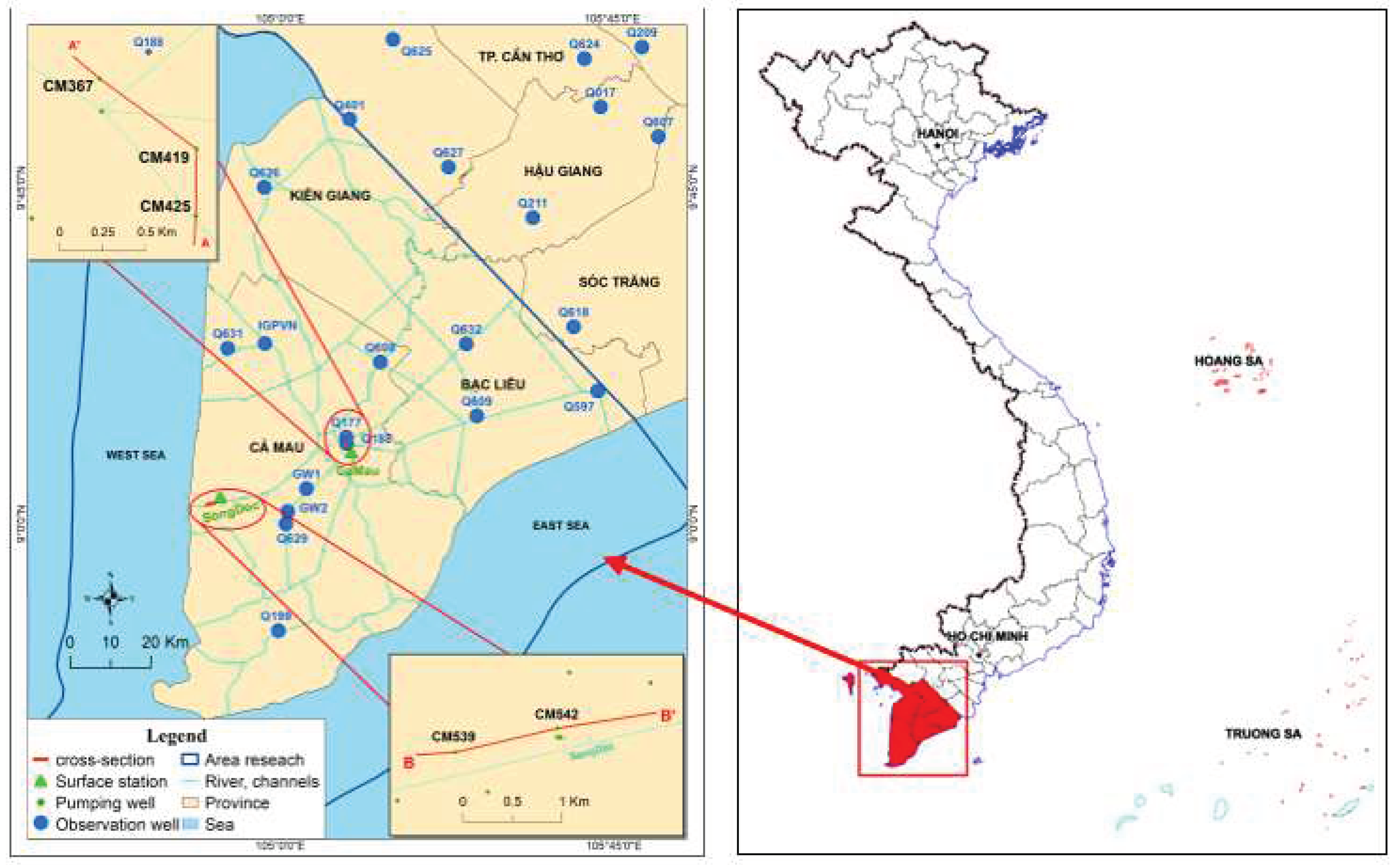
Figure 4.
Groundwater salinity data collected from households, exploitation wells, and monitoring wells in the period 2011 to 2021 (sources: NAWAPI, (Bauer et al. (2022), and IGPVN).
Figure 4.
Groundwater salinity data collected from households, exploitation wells, and monitoring wells in the period 2011 to 2021 (sources: NAWAPI, (Bauer et al. (2022), and IGPVN).
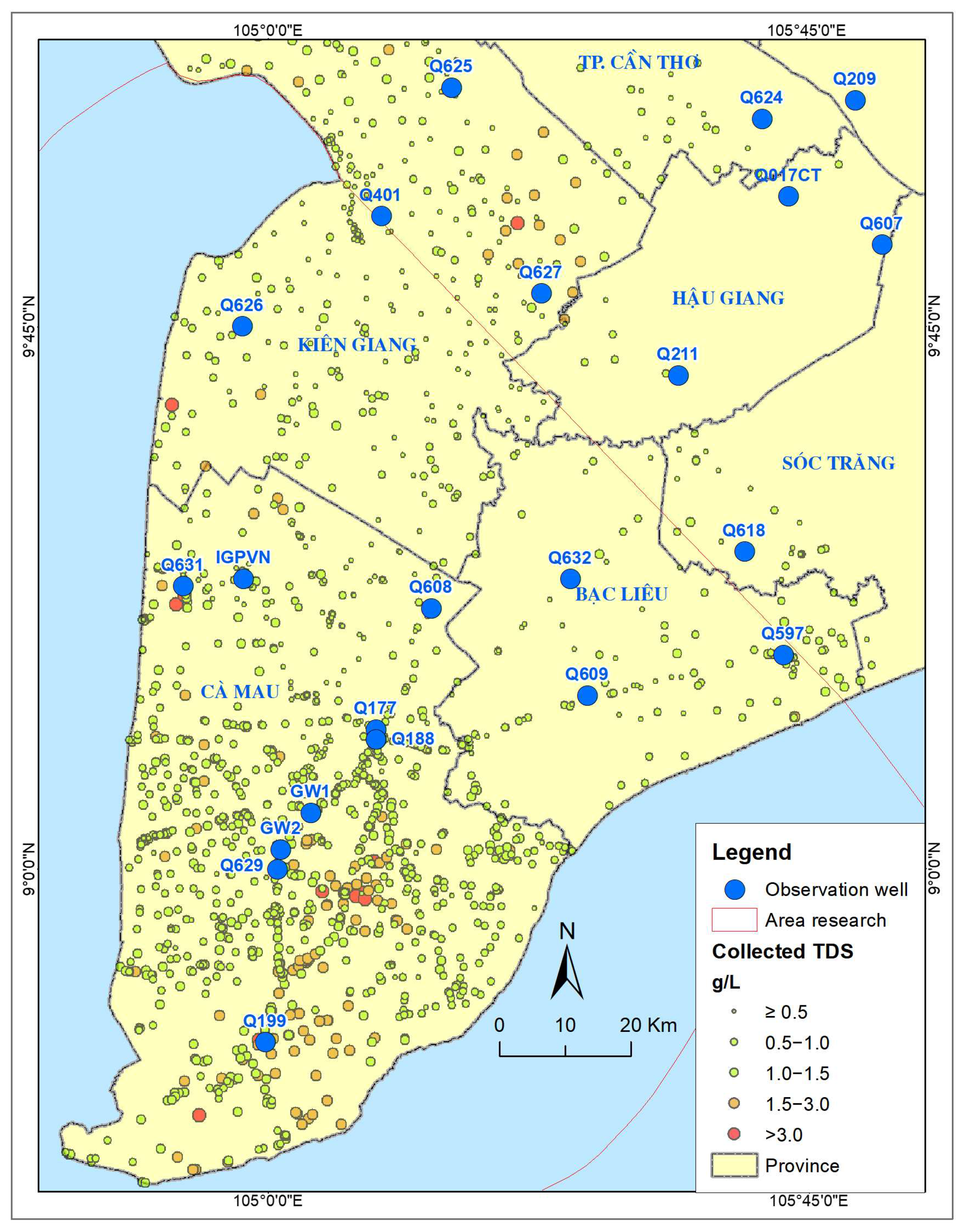
Figure 5.
Examples of TDS time series of groundwater monitoring wells from (a) NAWAPI (aquifer qh; period 2011-2023) and (b) the ViWaT project (well groups installed in 2022).
Figure 5.
Examples of TDS time series of groundwater monitoring wells from (a) NAWAPI (aquifer qh; period 2011-2023) and (b) the ViWaT project (well groups installed in 2022).
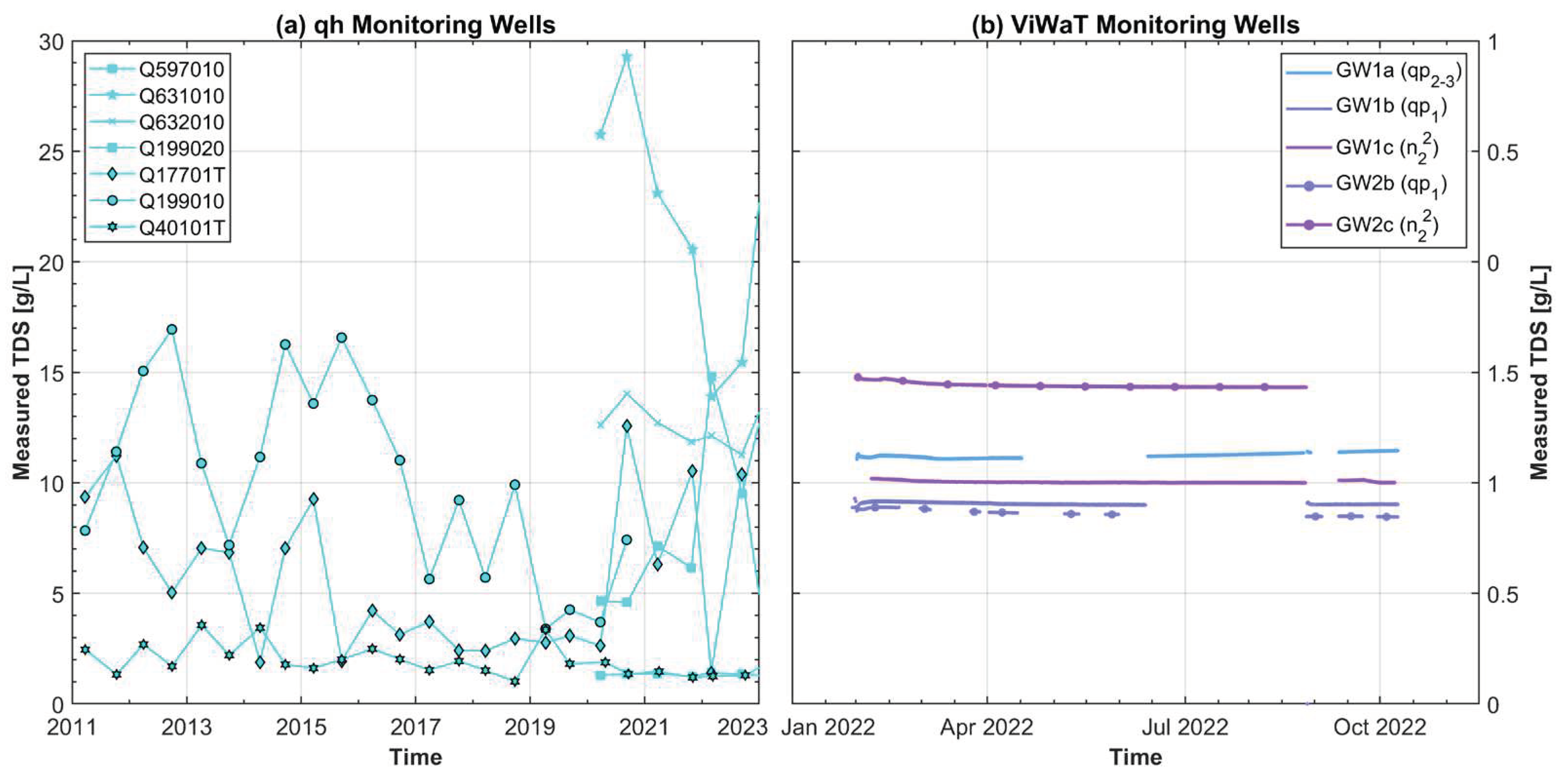
Figure 9.
Spatial distribution of initial salinity for the aquifers qh, qp3, qp2–3, qp1, n22, n21, and n13.
Figure 9.
Spatial distribution of initial salinity for the aquifers qh, qp3, qp2–3, qp1, n22, n21, and n13.
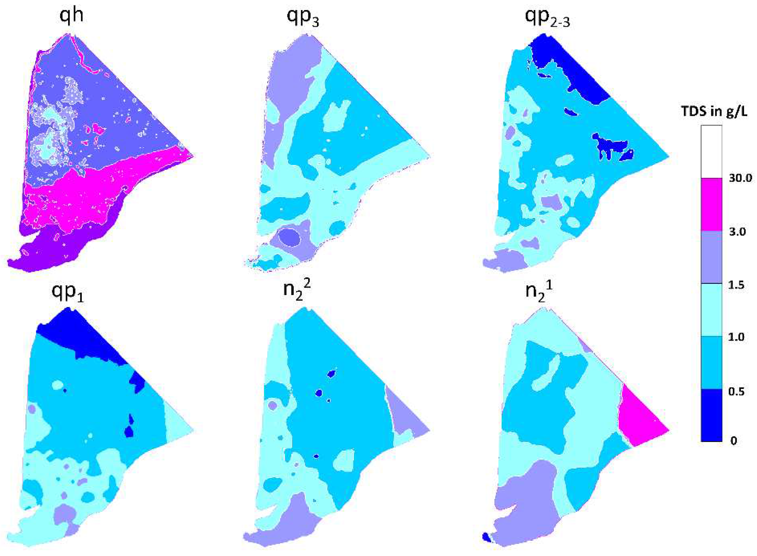
Figure 10.
(a) Dependence of dispersivity/flow meter in soil from Nilson Guiger and Monalisa Horvath (2003); (b) sediment grain-size-based classified regions for dispersion coefficients; (c,d,e,f) sediment-dependent dispersion coefficients for the aquifers qp2-3, qp1, n22 and n21 (Rinkel, 2022).
Figure 10.
(a) Dependence of dispersivity/flow meter in soil from Nilson Guiger and Monalisa Horvath (2003); (b) sediment grain-size-based classified regions for dispersion coefficients; (c,d,e,f) sediment-dependent dispersion coefficients for the aquifers qp2-3, qp1, n22 and n21 (Rinkel, 2022).
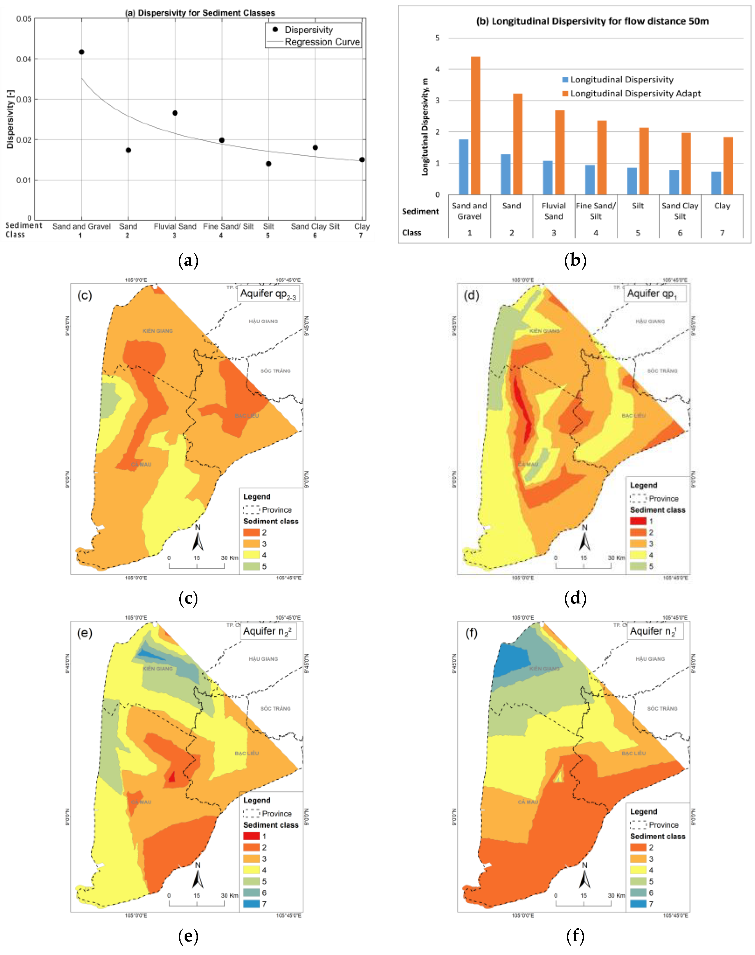
Figure 15.
The mean modeled TDS concentrations for qp3, qp2-3, qp1 and n22 under different Kz scenarios for pumping wells and observation wells (a) and temporal evaluation of TDS concentrations in pumping wells and observation wells in qp3 under different Kz scenarios (b).
Figure 15.
The mean modeled TDS concentrations for qp3, qp2-3, qp1 and n22 under different Kz scenarios for pumping wells and observation wells (a) and temporal evaluation of TDS concentrations in pumping wells and observation wells in qp3 under different Kz scenarios (b).
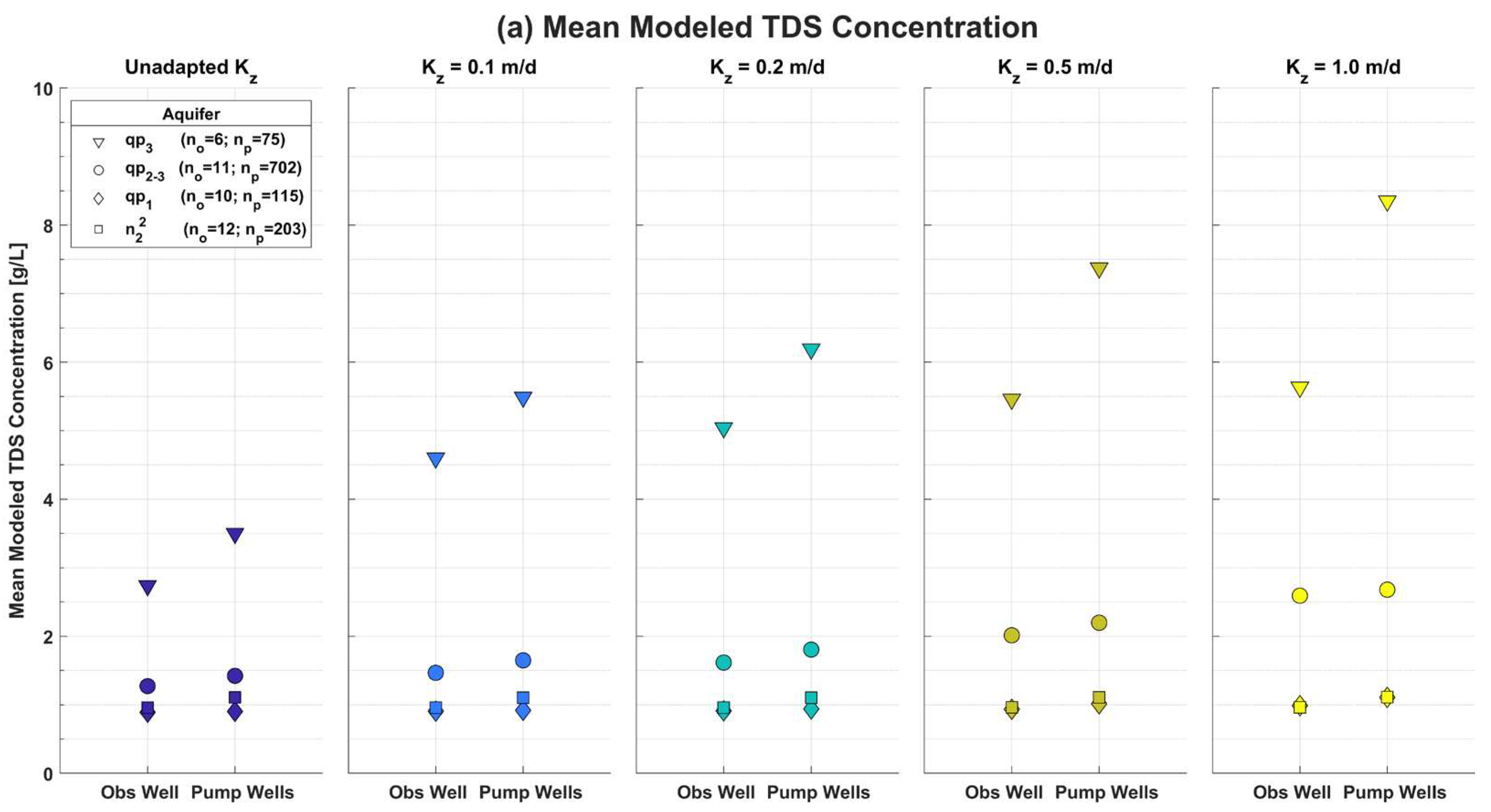
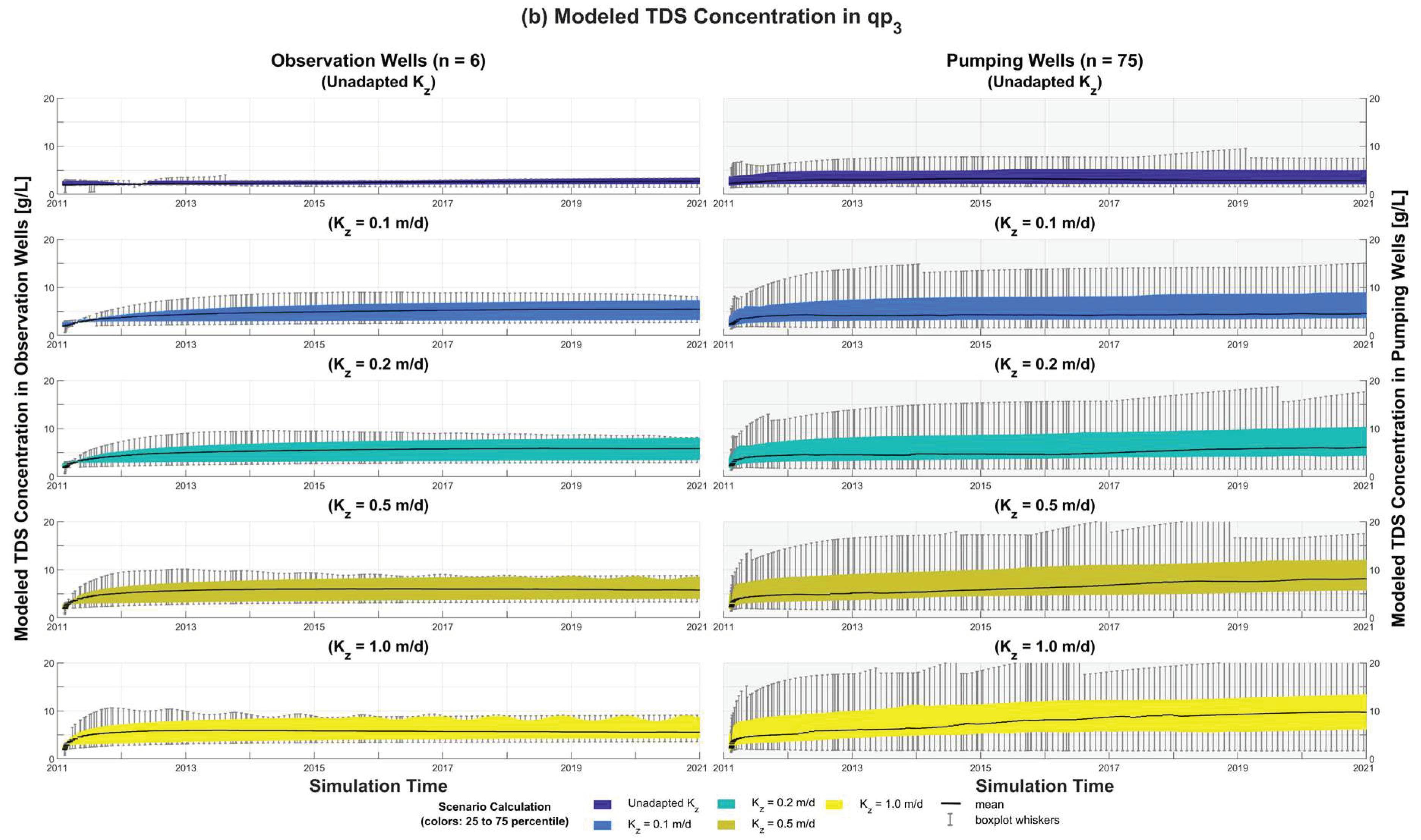

Table 1.
Available salinity time series with EC and TDS measurements and applied k values.
| Well with automatic EC measurement | Well with lab EC measurement | ||||||||
| Well name | aquifer | k(original) | k(corrected) | Well name | aquifer | k(original) | k(corrected) | ||
| Q631010 | qh | 0.82 | 0.70 | Q631050 | n22 | 0.45 | 0.50 | ||
| Q626020 | qp3 | 0.57 | 0.57 | Q632010 | qh | 0.55 | 0.55 | ||
| Q608030 | qp2-3 | 0.64 | 0.64 | Q632020 | qp3 | 0.52 | 0.52 | ||
| Q608040 | qp1 | 0.73 | 0.73 | Q632030 | qp2-3 | 0.51 | 0.50 | ||
| Q608050 | n22 | 0.57 | 0.57 | Q632040 | qp1 | 0.57 | 0.56 | ||
| Q608060 | n21 | 0.57 | 0.57 | Q632050 | n22 | 0.35 | 0.50 | ||
| Q609030 | qp2-3 | 0.57 | 0.57 | Q597010 | qh | 0.54 | 0.54 | ||
| Q609040 | qp1 | 0.86 | 0.70 | Q597040 | qp1 | 0.51 | 0.51 | ||
| Q609050 | n22 | 0.45 | 0.50 | Q597050 | n22 | 0.58 | 0.58 | ||
| Q609060 | n21 | 0.32 | 0.50 | Q199020 | qh | 0.4 | 0.5 | ||
| Q626030 | qp2-3 | 0.53 | 0.53 | Q199030 | qp1 | 0.6 | 0.6 | ||
| Q626040 | qp1 | 0.59 | 0.57 | Q19904T | n22 | 0.58 | 0.58 | ||
| Q626050 | n22 | 0.75 | 0.60 | Q19901Z | qp3 | 0.67 | 0.67 | ||
| Q631020 | qp3 | 0.63 | 0.63 | Q177040 | qp1 | 0.48 | 0.5 | ||
| Q631030 | qp2-3 | 0.40 | 0.52 | Q17704ZM1 | n21 | 0.52 | 0.52 | ||
| Q631040 | qp1 | 0.54 | 0.54 | ViWaT (GW1,2) | qp2-3, qp1, n22 | 0.51 | 0.51 | ||
Table 2.
Overview of dispersivity coefficients from different reports in Vietnam.
| Well Name | Aquifer | Longitudinal dispersity | Effective porosity | Specific storage | Average filtration velocity | Longitudinal dispersion coefficient | Flow distance | Location |
| αL (m) | ne (%) | (µ*) | V (m/min) | DL (m2/min) | m | |||
| CM2E (1) | n22 | 1.14 | 14.0 | 7.53 × 10⁻⁴ | 4.54 × 10⁻² | 8.54 × 10⁻⁴ | Ca Mau | |
| BL4D (2) | n22 | 0.02 | 16.0 | 4.58 × 10⁻³ | 4.20 × 10⁻³ | 8.40 × 10⁻⁵ | 8.0 | Bac Lieu |
| BL2B (3) | qp2-3 | 0.12 | 19.4 | 5.58 × 10⁻⁴ | 8.90 × 10⁻⁴ | 1.09 × 10⁻⁴ | 8.0 | Bac Lieu |
| IGPVN 1.4 (4) | n22 | 0.09–1.1 | 11.5–29.50 | 4.0–9.9× 10⁻⁵ | 10.09 | Ca Mau | ||
| CHN5 (5) | qp1 | 2.5 | 32.00 | 0.1736 | Hanoi |
(1) (DWRPIS, 2021a), (2) (DWRPIS, 2021b), (3) (DWRPIS, 2021c), (4) Pechstein et al., (2018), (5) Thanh et al. (2017).
Disclaimer/Publisher’s Note: The statements, opinions and data contained in all publications are solely those of the individual author(s) and contributor(s) and not of MDPI and/or the editor(s). MDPI and/or the editor(s) disclaim responsibility for any injury to people or property resulting from any ideas, methods, instructions or products referred to in the content. |
© 2023 by the authors. Licensee MDPI, Basel, Switzerland. This article is an open access article distributed under the terms and conditions of the Creative Commons Attribution (CC BY) license (http://creativecommons.org/licenses/by/4.0/).
Copyright: This open access article is published under a Creative Commons CC BY 4.0 license, which permit the free download, distribution, and reuse, provided that the author and preprint are cited in any reuse.


