
Submitted:
28 April 2023
Posted:
28 April 2023
You are already at the latest version
Abstract
Recharge is a crucial section of water balance for both surface and subsurface models in water resource assessment. However, quantifying its spatiotemporal distribution at a regional scale poses a significant challenge. Empirical and numerical modeling are the most commonly used methods at the watershed scales. However, integrated model inherently contain a vast number of unknowns and uncertainties, which can limit their accuracy and reliability. In this work, we have proposed integrated SWAT-MODFLOW and Transient Water Table Fluctuation Method (TWTFM) to evaluate the spatiotemporal distribution of groundwater recharge in Anyang wa-tershed, South Korea. Since TWTFM also uses SWAT model percolation output data, calibration was performed for individual models and coupled model. The coupled model was calibrated using daily streamflow and hydraulic head. SWAT-MODFLOW model performed well during the simulation of streamflow compared SWAT model. The study output showed that the study watershed had significant groundwater recharge variations during the simulated period. A sig-nificant amount of recharge happens in the wet season. It contributes about 34% of the average annual precipitation of the region. The direct flow components (surface and lateral) showed sig-nificant contributions when the water balance components were evaluated in the region. TWTFM showed a glimpse to estimate recharge, which requires representative monitoring wells in the study region. Comprehensively, the SWAT-MODFLOW model estimated groundwater recharge with reasonable accuracy in the region.
Keywords:
SWAT-MODFLOW
; groundwater recharge
; PEST
; Water table fluctuation
1. Introduction
Sustainable development and management of water resources are vital in watersheds that include urban and agricultural land use due to the rising demand for water supply, climate change, and improper management of water resources [1,2,3,4]. An Accurate understanding of the hydrological water cycle and its kinship system is mandatory to sustain and manage the water resources of the watershed [5,6]. It influences watershed recharge-discharge [6,7], water supply [8], and water quality. Further, a proper method for estimating water balance components is important [5,6,9]. Hence, this paper emphasis on assessing the groundwater recharge of the study watershed.
Preceding studies used several techniques to estimate groundwater recharge, which can be categorized into physical [10,11,12], tracer [13,14,15], and numerical methods [2,16,17]. Nonetheless, each method has its limitation while assessing recharge [11]. The numerical approach has become increasingly popular among researchers for evaluating groundwater recharge, which involves analyzing either surface or aquifer conditions, or both [18,19].
The Soil and Water Assessment Tool (SWAT) is usually applied to simulate surface water flow, while Modular Three-Dimensional Finite-Difference Ground-Water Flow Model (MODFLOW) is frequently employed for assessing unconfined groundwater flow. SWAT [20,21] has been extensively applied to determine surface and groundwater quality and quantity across various catchment scales. Further, it predicts how land use/cover and climate change influence designated catchment [9,18,22]. SWAT model have been applied in various hydrological watersheds for wide ranges of scale and multi-senior environmental studies [23,24,25]. For instance, SWAT model was applied in some parts of South Korea watersheds for water quality assessment [26], water balance analysis [27], and sustainability of water resources [28,29]. SWAT model places a strong emphasis on surface processes, but its ability to simulate groundwater flow is inadequate by its lumped nature [30]. Various strategies have been proposed to address the limitations of the original SWAT groundwater module, including altering the code of the module [31], implementing a more intricate groundwater storage module [32], or substituting the non-shallow aquifer with the grid cell aquifer [33]. Though, limited to simulating groundwater flow accurately due to semi-distribution approach. MODFLOW model is a suitable option for groundwater flow simulation since it is distributed and physically based, which was the limitation of SWAT model. This model considers various boundary conditions to simulate groundwater flow processes; such package includes Recharge, River, Reservoir, Well, and others [34]. It was also applied to investigate the influence of sub-surface water abstraction on surface water resources [35,36]. However, it is inadequate in hypothesizing surface water flow [9,18]. Hence, coupled SWAT-MODFLOW approach is critical to overcoming the drawbacks of models and for a better representation of the hydrological system [37].
Integrating SWAT and MODFLOW models was initially introduced by Sophocleous et al. [38] and has been upgraded while comparing the model performance with SWAT model [18,39,40]. In the integrated model framework by Bailey et al. [41], SWAT model focuses on simulating the surface hydrological processes, while MODFLOW-NWT (Newton-Raphson formulation for MODFLOW) [42], which is capable of solving unconfined aquifer sub-surface water flow problems, simulates groundwater flow processes. According to Wang et al. [43], preceding studies by the SWAT-MODFLOW model can be classified into non-situational and situational simulations. Non-situational state studies are primarily focused on streamflow simulation, groundwater discharge, surface water-groundwater interaction, and regional water balance [39,41,44,45,46,47], while situational scenario simulation studies using SWAT-MODFLOW consider the influences of groundwater abstraction on the surface water resources [9,48,49].
As specified by Ntona et al.[34], SWAT-MODFLOW is the most applied model for surface-groundwater analysis from the period 1992 to 2020 worldwide and it continues to be the keystone for recent studies. For instance, a study by Mosase et al. [50] estimates the spatio-temporal distribution of recharge, water table level, and interaction between surface and sub-surface water in the Limpopo River Basin, Africa. Sophocleous and Perkins [51] use SWAT-MODFLOW to three basins in Kansas, USA watershed to explore abstraction impacts on streamflow and water table levels. They also analyze the outcome of various scenarios, including climate change on water resources. A study by Gao et al. [39] analyzed spatiotemporal variations of the surface water resources applying integrated model in the River catchment, USA. Taie Semiromi and Koch [18] utilize the integrated model to inspect surface and subsurface water interaction in an agricultural watershed in Iran. They point out that climate change alone does not create future water scarcity but rather the overutilization of the groundwater source in the study of the agricultural watershed. Chunn et al. [52] apply the same model to evaluate consequence of climate variation and groundwater abstractions on the surface water-groundwater interaction in western Canada. They pinpoint that in the reduction of river flow and groundwater level, the overuse of groundwater contributes a high role, as stated by [45,53]. In recent hydrological studies, parametrization tools have been applied for SWAT-MODFLOW model, which reduces the uncertainty of parameters applied for the calibration of the model [30,54]. For instance, Liu et al. [30] applied PEST (parameter estimation by sequential testing) as calibration tools for integrated model and evaluate the streamflow response to groundwater abstractions for the Uggerby River Catchment in northern Denmark. SWAT-MODFLOW has a significant advantage in simulating interconnected surface-groundwater scenarios; such as in the case of streamflow evaluation, it showed high precision [9,30,41,46]. However, numerical models like SWAT-MODFLOW always have uncertainty [55]. Environmental models, especially those at the regional scale often suffer from significant uncertainty due to the large number of unknown factors. The source can be from model structure, input database, or parameterization options [43]. For example, Guevara-Ochoa et al. [44] mentioned SWAT model transfers a higher recharge amount to MODFLOW during the wet season since SWAT-MODFLOW does not have a module to associate the alteration among groundwater and soil saturation. While there are many other recharge estimation methods, water table fluctuation method is optioned as additional approach.
Among the many methods for estimating groundwater recharge, water table fluctuation (WTF) is a straightforward, accurate, and simple method [11,12,56]. The method required observed groundwater level data series and aquifer parameters, which can be determined using various methods [11,12,57]. To reduce subjectivity and increase efficiency several modifications have been taken to this method [58,59,60]. One of the approaches was to link the WTF method with a hydrological model, such as SWAT model, which helps to overcome local representation of the method. For instance, Chung et al. [59] estimated recharge by linking SWAT model with TWTFM in Hancheon watershed, Jeju Island, South Korea. Moreover, deep percolation (recharge from SWAT) was used as input for TWTFM to determine aquifer parameters (reaction factor and specific yield) for TWTFM. Applying an alternative approach to estimating groundwater recharge is recommended since it assures results [12,56,61,62]. This study aims to apply SWAT-MODFLOW model and TWTFM method to assess the groundwater recharge in our study area. As per our knowledge, no research has been reported to use coupled model and TWTFM to evaluate groundwater recharge and it will be presented for the first time in our study.
In this study, we proposed numerical and empirical methods to evaluate the spatiotemporal distribution of groundwater recharge. The spatial and temporal distribution of groundwater recharge using SWAT-MODFLOW model is evaluated for the study watershed. Further, we approach recharge estimation using TWTFM as an alternative option and evaluate the output with numerical model approach. Seasonal variation of groundwater recharge of the region is presented. Furthermore, the water balance segments are acquired and discussed.
2. Materials and Methods
2.1. Description of Study Region
Anyang watershed is located in northwestern South Korea which is displayed in Figure 1. The study watershed covers an approximately 137 km2 area and drains into the Han River, one of the longest rivers in the Korean Peninsula. The altitude ranges from 11–59l m above mean sea level and an average of 116 m for the region. Between 2002 and 2018, the mean annual precipitation was 1266.8 mm, and the yearly averages for the lowest and peak daily temperatures were 8.5 and 17.5 ℃, respectively. For a while, the streams of the study region are gauged that started before 2002. During the summer period, the streamflow gets its maximum value.
Anyang watershed land use/land cover consist of most forest and urban, with forest enclosing approximately 50% of the whole area and urban-industrial areas covering 43%. The remaining 7% is comprised of pasture, water bodies, wetlands, and agricultural land use. The land use was classified into 14 classes by the SWAT model, as represented in Figure 2.
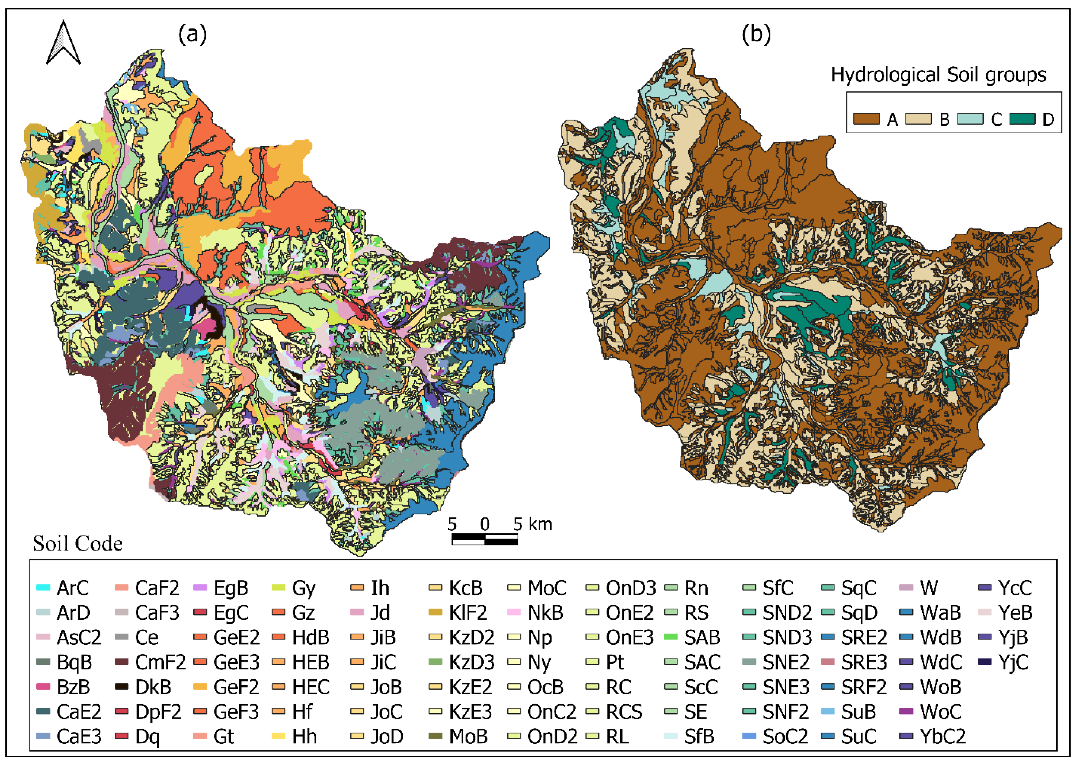
The soil types and hydrological soil groups of the study are displayed in Figure 3. In the study area, most soil types have four layers, the highest depth varies between 60 and 2000 mm. Hydrological soil group “A” dominates the region with 67.1%, which characterizes the soil texture of sand and sandy loam with low runoff potential. Then followed by soils that have a hydrological group of “B” with 27% coverage in the region, which encompasses loam and silt loam soils with moderate infiltration potential characteristics. Soil hydrological group “C” includes sandy clay loam soil, soil group “D” comprises clay, clay loam, and sandy clay soils. Hydrological soil group “C” comprises approximately 3.2% and “D” 2.7%. Both hydrological soil groups “C” and “D” are characterized by low seepage and a high potential for surface runoff. They mainly occupy the lowland zone, including wetlands and water bodies.
The information of Soil types and LULC of the study watershed were obtained from the National Institute of Agricultural Sciences and the Ministry of Environment of Korea, respectively. Daily streamflow data and weather data were provided by Water Resources Management Information System [63] and Metrological Agency Weather Data Service [64] respectively.
Figure 3.
Anyang watershed soil types: (a) Soil classes applied in SWAT model (the whole information can be retrieved from [65] website); (b) hydrological soil groups.
Figure 3.
Anyang watershed soil types: (a) Soil classes applied in SWAT model (the whole information can be retrieved from [65] website); (b) hydrological soil groups.
2.2. Evaluation of Recharge Using Integrated Model and Transient Water Table Fluctuation Method
2.2.1. SWAT-MODFLOW Model
SWAT model ability to address groundwater flow is restricted by its aggregated nature, while MODFLOW struggles to estimate surface water condition, which is a critical input for the groundwater model because it lacks a land surface hydrology model. However, integrated SWAT-MODFLOW model overcomes the limitation by replacing the SWAT model module for groundwater with the MODFLOW [43,48].
During simulating the groundwater recharge using SWAT-MODFLOW model, data transfer from individual model is vital for accurate estimation. The data transfer between individual models uses a mapping scheme. The simulated deep percolation of SWAT model (HRUs) mapped as recharge to the Disaggregated HRUs (DHRUs), MODFLOW in each grid cell, while SWAT model will get groundwater discharge in each sub-basin from MODFLOW [41]. SWAT model uses equation (1) to simulate deep percolation (groundwater recharge).
 where ωrchrg,i is the quantity of water inflow to the aquifers as recharge on day i (mm), δgw (days) is lapse period of the aquifer materials, ωseep is the sum quantity of water exiting below soil profile on day i(mm), and ωrchrg,i-1 is the quantity water inflow to the aquifers as recharge on dayi-1 (mm).
MODFLOW uses a finite difference approach as stated in equation (2) to describe the groundwater flow at grid level. MODFLOW model discretizes the aquifer into grid cell level, which can be defined in terms of rows, columns, and layers. Simulation such as groundwater head presented in grid cell level for the model. After the SWAT-MODFLOW setup is completed, SWAT groundwater module will be deactivated and MODFLOW groundwater flow equation used in the case of recharge.
 where h is the hydraulic head (m). Kxx, Kyy, and Kzz signify the hydraulic conductivity (m.day-1) along x, y, and z directions, respectively. The Ss is the specific storage of the aquifer that is a dimensionless quantity, t (day) represents time, and where W (day-1) signifies the source or sink. If the W is positive, it represents the recharge into the aquifer, while if it is negative it represents abstraction.
2.2.2. Transient Water Table Fluctuation Method (TWTFM)
Water table fluctuation (WTF) method has been utilized in various studies due to its easiness and straightforwardness to apply [67,68,69] and the method described in detail by [12]. The basic concept of this method, the rise of groundwater in the aquifers occurs due to the percolation process in the region. Several monitoring groundwater level data are required to apply this method with specific yield values of the aquifer. For accurate estimation of recharge, specific yield value should be acceptable [12,70,71]. Some studies use regression approaches to estimate specific yield, by developing a relationship between groundwater fluctuation in response to series event precipitation [72]. To calculate recharge with time series, researchers acquire inverse modeling of the water table elevation with temporally changing specific yield [60,71]. However, determining the aquifer parameters, including specific yield from known recharge (especially from numerical model approach), reduces the uncertainty of aquifer parameters value [59,73].
De Zeeuw and Hellinga (1958) suggested analytical equation (3) to determine recharge and discharge during transient state subsurface drainage process [74]. In the present study, we implemented this equation to estimate recharge. The procedure to determine recharge using this method is described in Figure 4. First, prepare selected groundwater (GW) level series data (daily), which should be continuous and reliable. Then determine reaction factor (α) parameter using equation (4) which is solely dependent on observed water level data series. Sum up simulated percolation from the SWAT model and use it for alteration input. Iterate specific yield (μ) value until the sum of SWAT percolation and computed recharge using TWTFM values close to each other.
 where α denotes the reaction factor (d-1), μ is the specific yield of the aquifer, hi is the GW level (L) on the i day, hi-1 is the GW level (L) on the i-1 day, Δt is the time interval (T), and R∆t is average recharge for time interval t-1 to t, and was presumed constant.
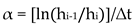
Reaction factor (α) can be calculated based on equation (4), which depends only on the groundwater level data and assumes no recharge in the aquifer [74]. Specific yield (μ) was determined using equation (3) and iteration procedure. Detailed procedure the for TWTFM approach reported by Chung et al. [59].
For this study, seven monitoring wells with reliable and long-period records were selected to apply TWTFM approach as shown in Figure 5. We applied this method even if the selected monitoring wells were not well distributed in the study watershed. Therefore, the number of wells and their distribution were considered a limitation of the TWTFM approach for this study. The whole process and workflow of the method is stated in Figure 4.
2.3. Model Setup and Coupling
2.3.1. SWAT Model
To build the study area, SWAT2012 (ver.636) was employed. SWAT model, is a semi-distributed model, which functions on a daily time series. A digital elevation model (DEM) was applied to delineate into watershed and sub-watershed (subbasins). For this model, the landscape is classified into conceptual units named Hydrological Response Units (HRUs). A piece HRU signifies an area of the landscape that has similar soil, land use, slope, and management characteristics. The SWAT model simulates the quantity and quality of water resources based on the conceptual units (HRUs)[75]. To adjust the model size without missing essential data, setting the proper number of HRUs is a vital procedure [76]. SWAT model has multiple HRU definition options, which allow users to represent the variability of LULC, soil types, and topography within the study watershed. In the present study, multiple HRUs option with threshold values of 5% was optioned to create the HRUs of the watershed.
QSWAT is a graphical user interface (GUI, version 3.22) that was utilized to construct and run the SWAT model of the study watershed. The region was delineated and divided into 21 subbasins (Figure 1) using a 30 m resolution digital elevation model (DEM). Stream network was constructed to duplicate the water network of the study area. Then 1679 HRUs were created with multiple HRUs option. For streamflow calibration, station gauge (SG2) (Figure 1) was used for this study. Weather data were imported and written in the model. From 2006 to 2018, the SWAT model simulation was performed; the initial three years (2006–2008) were designated as a warm-up period, during which the model did not provide results for analysis or interpretation.
2.3.2. MODFLOW Model
The study region conceptual model was developed using the GMS software MODFLOW, version 10.5.8. MODFLOW is employed to solve the groundwater flow of the aquifer in three dimensions finite difference approach [77]. To account for changes in the wetness and confinement of the grid cells over time, this study utilized the MODFLOW-NWT (Newtonian Solver) engine. MODFLOW-NWT is preferred over other versions of MODFLOW due to its ability to simulate hydraulic heads for dry cells without changing them to inactive cells in an unconfined aquifer [42]. In addition, upstream weighting (UPW) package was used, which enables zero magnitude for dry cells flow out and determines the head from the inflow to the dry cells. Overall, utilization of MODFLOW-NWT enables a more accurate analysis of sub-surface water flow for the study watershed [42].
Anyang watershed (with 137 km2 coverage) was discretized into grid cells with a lateral resolution of 100 m by 100 m, which resulted in 17,465 active grid cells. Conceptual top elevation data was obtained from SWAT model, DEM raster file. The bottom elevation was determined using data from electrical resistivity tests conducted in the study watershed; elevation ranges 50–200 m below the surface. The stream network created during delineation SWAT process was introduced to MODFLOW as a shape file. Using the river package 825 stream cells were created for the watershed.
During the simulation of steady-state groundwater flow, parameters include hydraulic conductivity, river conductance, initial head, and sources and sinks. Recharge rate was obtained from SWAT percolation output, which provides a single value for MODFLOW. The initial head values were acquired by interpolating from 35 monitoring wells data collected in the study region. To attain initial values for hydraulic conductivity interpolation approach was used. As anticipated, the initial simulation revealed a discrepancy between the observed and calculated head. The conceptual model was calibrated by the Parameters ESTimation (PEST) algorithm, which involved adding more pilot points in areas where data was limited. During calibration, the pilot points were comprised by fixing the minimum and maximum hydraulic conductivity to the same values.
After achieving reasonable results between the observed and computed head during the steady-state simulation, a simulation setup for the transient state was initiated. Before proceeding with the coupling procedure between SWAT and MODFLOW, specific storage and specific yield parameters were established for the transient simulation.
2.3.3. SWAT-MODFLOW Model Integration
The linking code, which integrates both SWAT and MODFLOW models in daily time steps, was introduced by Bailey et al. [41]. It has significant advantages for the models since the coupling approach enables the models to share their computed results without having to rewrite or import their input data. One of the significant steps during the coupling procedure is converting SWAT HRUs to disaggregated Hydrologic Response Units (DHRUs), which conjunction with a MODFLOW grid shape file, to provide spatially explicit information for the model. The procedure made available by Park et al. [78] explains the entire step for creating and transferring the current linking files and integrating the model.
In the present study, QSWATMOD, a QGIS-based graphical interface, was applied to do before processing, configuration, and after processing for coupled model. It is written in Python code, which is suited to create linkage files between SWAT and MODFLOW. The fundamental procedures are described by Bailey et al. [41].
To perform integrating using QSWATMOD, the following inputs are required, SWAT output file, shape files of subbasin, HRU, and river network, and a MODFLOW model folder as native text as a pre-processing procedure. Stream network can be selected from either SWAT or MODFLOW model. For this study, the MODFLOW stream was chosen due to modification of the riverbed conductance. To link the models, DHRUs were created to intersect with MODFLOW grid cells. A zonal polygon was created for aquifer parameters in the MODFLOW model before the coupling process, which can be used during the calibration process of SWAT-MODFLOW. All integrated model files were stored in a single working directory.
2.4. Model Calibration and Performance Evaluation
2.4.1. SWAT Calibration
SWAT model is suitable for simulating streamflow, it can be validated with observed streamflow data. Parameters that influence simulated streamflow should be calibrated until it sounds with observed streamflow values. To do that SWAT-CUP program was applied with the Sequential Uncertainty Fitting program (SUFI-2) algorithm, which considers all roots of uncertainty related to the model, parameters, and input data [79]. Details description of SUFI-2 and other algorithms was explained by [80]. In this work, the simulation of the SWAT model covered 13 years, with the calibration period from 2013 to 2018 and the validation period from 2009 to 2010. In our study, calibration and validation for the observed streamflow were in the daily time series.
From several SWAT hydrological parameters, sensitive parameters were chosen to calibrate the model by providing the acceptable range value. Selected parameters control simulated soil water, surface runoff, evaporation, and groundwater. Detailed descriptions of selected parameters were stated in Table 1.
During calibration, the execution of the model can be assessed using statistical parameters like the Nash-Sutcliffe efficiency (NSE) and the regression coefficient (R2) values [81]. NSE Value higher than 0.5 is acceptable for calibration performance. For NSE nearer to one indicates that the model outputs are significantly nearer to observed data. The regression coefficient (R2) is applied to determine how closely observed and simulated data align. In this study, NSE was selected as the objective function to evaluate the model simulation during the calibration and validation period in SWAT-CUP program. As stated in Figure 1, the study watershed has two stream gauges (SG1 and SG2). Calibration was implemented at SG2 since the other stream gauge has missing data, which makes it difficult to select. For subbasins, where SG2 did not cover regionalization approach was used [82].
2.4.2. SWAT-MODFLOW Model Calibration
The process of acquiring suitable parameters value is essential in modeling process since it helps in the accuracy of the model output. Previous studies have approached several calibration and validation frameworks for SWAT-MODFLOW. The first is to calibrate using automated parameter estimation tools for both SWAT and MODFLOW independently and then recalibrate the integrated model manually [9,22]. The other option is to use automated and semi-automated calibration approaches for coupled model [30,40,83].
SWAT-MODFLOW calibration using PEST framework was first introduced by [84]. In the present work, a parallel implementation of PEST called BEOPEST was used, which minimize the time needed for calibration. The PEST framework requires five types of files to run; control file, PEST-executable file (BEOPEST), model batch file, model input template file, and instruction file (for model output). Detail descriptions about the procedure can be found [30].
To improve streamflow simulation further five parameters from SWAT were selected for recalibration. Aquifer parameters (HK, SS, and Sy) were included in the calibration processes of SWAT-MODFLOW. Table 2 describes the selected parameters for calibration with their value ranges.
3. Results and Discussions
3.1. Calibrated Parameters
In this section, the final automated parameters used for integrated SWAT-MODFLOW model were presented. Parameters in Table 3 have lower values compared to the SWAT model calibration parameters value displayed in Table 1. One of the possible reasons for this is to overcome the simulated streamflow lower base flow and peak flow conditions and the statement supported by [85]. Zonal polygons were created preceding to coupling process based on hydraulic head distribution to calibrate aquifer parameters. Figure 6 showed the final automated aquifer parameter value ranges of the study region. Calibrated hydraulic conductivity value range from 0.014 m/day to 0.68 m/day. Yifru et al. [9] reported the hydraulic conductivity range between 0.001 m/day to 26 m/day for three watersheds that include the present work region. They also reported specific storage and specific yield values as 0.0001 m-1 and 0.18, respectively. For this study, specific storage values range from 0.0017 m-1 to 0.01m-1, and specific yield range from 0.03–0.41. Referring to Figure 6, we can draw a relationship between individual aquifer parameters. For example, specific yield and specific storage have inverse relations during calibration of the hydraulic head of the study watershed.
3.2. Model Performance during Calibration and Validation
Figure 7 describes daily streamflow between simulated and measured for SWAT and integrated model. The streamflow was calibrated from 2013–2018 and validated from 2009–2010. Table 4 summarizes model performance statistics of NSE and R2 between measured and calculated streamflow for SWAT and SWAT–MODFLOW model. During the integrated model, better performance statistics showed for streamflow than the SWAT model, as stated in Table 4. SWAT-MODFLOW model performs better simulation during low base flow and peak flow conditions of observed streamflow, as shown in Figure 7. According to the evaluation criteria mentioned by [86], both models accomplished well in simulating the streamflow during calibration and validation set time.
The hydraulic head simulation was performed based on the continuity of recorded monitoring wells. Several of the observed wells in our study do not have continuous daily time series data, which is considered a limitation of our study in the region. The selected monitoring wells have records from May 2017 to September 2018. Figure 8 describes the hydraulic head of the study watershed. The calculated depth to water values was compared with the observed, as displayed in Figure 8a. The negative sign indicates that the water level is level below the ground level. As shown in Figure 8a, good trends were visualized between observed and calculated groundwater levels, with the difference between the heads less than 1 m. Figure 8b displays the spatial distribution of simulated hydraulic head of our study watershed. The hydraulic head ranges from 9.7 m to 453.5 m (Figure 8b). The middle part of the study region shows low hydraulic heads while most of the north and east area have higher values.
3.3. Groundwater Recharge
Figure 9 displays the distribution of average groundwater recharge during the whole simulation period (2009–2018). The figure demonstrates a considerable spatial and temporal distribution of groundwater recharge in the watershed. The monthly average recharge distribution describes these patterns in the area that ranges from 0–22.4 m3/day (Figure 9a). In the present work, the groundwater recharge amount is complicatedly distributed and problematic to connect with the physical topographies of the region, even though the northeast has a maximum recharge. The study area precipitation was intense during the wet season of the summer period (June–August), and the groundwater recharge shows this tendency (Figure 9c). During the wet season, the average recharge ranges from 0–58.6 m3/day. In the region, the dry season (January–March) shows the lowest value among a yearlong recharge. During this season, most areas get the lowest recharge and the highest value is 4.5 m3/day (Figure 9b). Topography with high elevation shows relatively high recharge values.
Yifru et al. [9] stated that the recharge covers 18% of the annual average precipitation in the Han River watershed which includes our study region. Further, the peak and significant amount of recharge happen in the course of the summer period, and July month has the largest recharge value. In the present study, the groundwater recharge covers 34 % of the average annual precipitation of the region. Even though, it is not indicated numerically similar recharge pattern was shown graphically in this study region by Yifru et al. [9]. Whereas, the minimum recharge occurs during a month of the winter season with the highest value of 8.85 mm.
Table 5 shows the simulated recharge amount using the TWTFM approach. In addition, it listed the estimated parameters (specific yield and reaction factor) in the selected subbasin of the study region.
Groundwater level records and initial recharge input data are essential to apply the transient water table fluctuation method. From available monitoring wells in our study, seven were selected to apply TWTFM approach. For initial recharge input, SWAT percolation values at subbasin level where observed wells exist. For this method, recharge was estimated from May 2017 to September 2018. Table 5 describes the calculated aquifer parameters and recharge for selected monitoring wells in the study watershed. Specific yield ranges from 0.0078–0.022, while the reaction factor ranges from 0.04 d-1 to 0.2 d-1. The specific yield values were considered as initial input values in calibration of coupled model. Estimated recharge ranges between 553.6 mm to 1020 mm for this method, which is shown in Table 5. TWTFM provides almost similar results of recharge with SWAT model. For SWAT-MODFLOW, the average annual recharge was 430 mm for the whole watershed. For this method to draw a representative recharge value for the study watershed, well-distributed monitoring wells are required, which consider a limitation (Figure 5).
3.4. Water Balance Components of Study Watershed
Figure 10 illustrates the major water balance segments from integrated model for the period 2009–2018 (until September). Percolation is the major contributor to the water cycle of the study region. Based on Figure 10, the maximum monthly percolation occurs in June 2011 with 11.7 mm value where the precipitation was also maximum. Further, surface runoff and lateral flow show similar peak values during this time. The yearly average evapotranspiration is around 252 mm, almost 20% of the annual precipitation of the region. The direct flow components (surface and lateral) were significant, which is around 45% of the annual precipitation in the watershed. The groundwater volume shows decreasing pattern to adjust the initial hydraulic head of the region.
4. Conclusions
Numerical model and empirical approach were utilized to evaluate the groundwater recharge of Anyang watershed. A numerical model, SWAT-MODFLOW, was used to assess the spatiotemporal groundwater recharge distribution of the study region. Observed streamflow and groundwater level were calibrated for the coupled model. Streamflow was calibrated from the year 2013–2018 and validated from 2009–2010. The performance of the model was evaluated using statistical parameter function of R2 and NSE. The integrated model showed better performance in simulating the streamflow during calibration and validation period. Re-calibration of selected SWAT parameters was a proven reason for better streamflow simulation for integrated model, other than aquifer parameters calibration. Monitoring wells were evaluated with calculated water level below the ground level, which showed a good trend with the measured value.
SWAT-MODFLOW model quantified the average monthly groundwater recharge in the region and showed the spatiotemporal distribution variations yearlong. Seasonal recharge in the region was well spotted in the model and a significant difference was shown between the dry and wet seasons. The groundwater recharge contributes 34% of the annual average precipitation even though the region has large urban area coverage. The contribution of the direct flow component (surface and lateral) was significant, which relates to the geological characteristics of the study region.
The other method applied to evaluate recharge was the transient water fluctuation method (TWTFM). Seven monitoring wells with long-term record daily series were selected for this method. It provides recharge that ranges from 553.6–1020 mm and aquifer parameters that were used as initial input during calibration of coupled.
In general, the present work showed the utilization and performance of the SWAT-MODFLOW model and TWTFM approach to analyze groundwater recharge. SWAT-MODFLOW shows the spatial and temporal distribution of the groundwater recharge of the study watershed. Hence, it provides a better representation of the surface water and groundwater of the region. TWTFM shows a glimpse as an alternative option for recharge estimation, but it requires well-distributed groundwater level data to represent recharge condition of the region.
Author Contributions
Conceptualization and methodology, H.H.W., T.D.M., B.A.Y., S.W.C., and I.-M.C.; validation, H.H.W. and B.A.Y.; resources and data curation, S.W.C. and I.-M.C.; writing- original draft preparation, H.H.W.; writing-review and editing, H.H.W., T.D.M., B.A.Y., S.W.C., and I.-M.C.; supervision, I.-M.C.; project administration, I.-M.C.; funding acquisition, I.-M.C. All authors have read and agreed to the published version of the manuscript.
Funding
Acknowledgments
Conflicts of Interest
The authors declare no conflict of interest.
References
- Aslam, R.A.; Shrestha, S.; Usman, M.N.; Khan, S.N.; Ali, S.; Sharif, M.S.; Sarwar, M.W.; Saddique, N.; Sarwar, A.; Ali, M.U.; et al. Integrated SWAT-MODFLOW Modeling-Based Groundwater Adaptation Policy Guidelines for Lahore, Pakistan under Projected Climate Change, and Human Development Scenarios. Atmosphere (Basel). 2022, 13, 2001. [Google Scholar] [CrossRef]
- Arshad, A.; Mirchi, A.; Samimi, M.; Ahmad, B. Combining Downscaled-GRACE Data with SWAT to Improve the Estimation of Groundwater Storage and Depletion Variations in the Irrigated Indus Basin (IIB). Sci. Total Environ. 2022, 838. [Google Scholar] [CrossRef] [PubMed]
- Locatelli, L.; Mark, O.; Mikkelsen, P.S.; Arnbjerg-Nielsen, K.; Deletic, A.; Roldin, M.; Binning, P.J. Hydrologic Impact of Urbanization with Extensive Stormwater Infiltration. J. Hydrol. 2017, 544, 524–537. [Google Scholar] [CrossRef]
- Barron, O.V.; Donn, M.J.; Barr, A.D. Urbanisation and Shallow Groundwater: Predicting Changes in Catchment Hydrological Responses. Water Resour. Manag. 2013, 27, 95–115. [Google Scholar] [CrossRef]
- Fleckenstein, J.H.; Krause, S.; Hannah, D.M.; Boano, F. Groundwater-Surface Water Interactions: New Methods and Models to Improve Understanding of Processes and Dynamics. Adv. Water Resour. 2010, 33, 1291–1295. [Google Scholar] [CrossRef]
- Sophocleous, M. Interactions between Groundwater and Surface Water: The State of the Science. Hydrogeol. J. 2002 101 2002, 10, 52–67. [Google Scholar] [CrossRef]
- Sharp, J.M. The Impacts of Urbanization on Groundwater Systems and Recharge. Aquamundi 2010, 1, 51–56. [Google Scholar]
- Wang, Y.; Zheng, C.; Ma, R. Review: Safe and Sustainable Groundwater Supply in China. Hydrogeol. J. 2018, 26, 1301–1324. [Google Scholar] [CrossRef]
- Yifru, B.A.; Chung, I.M.; Kim, M.G.; Chang, S.W. Assessment of Groundwater Recharge in Agro-Urban Watersheds Using Integrated SWAT-MODFLOW Model. Sustain. 2020, 12, 6593. [Google Scholar] [CrossRef]
- Lee, C.H.; Yeh, H.F.; Chen, J.F. Estimation of Groundwater Recharge Using the Soil Moisture Budget Method and the Base-Flow Model. Environ. Geol. 2008, 54, 1787–1797. [Google Scholar] [CrossRef]
- Scanlon, B.R.; Healy, R.W.; Cook, P.G. Choosing Appropriate Techniques for Quantifying Groundwater Recharge. Hydrogeol. J. 2002, 10, 18–39. [Google Scholar] [CrossRef]
- Healy, R.; journal, P.C.-H. ; 2002, undefined Using Groundwater Levels to Estimate Recharge. Springer 2002, 10, 91–109. [Google Scholar] [CrossRef]
- Chand, R.; Chandra, S.; Rao, V.A.; Singh, V.S.; Jain, S.C. Estimation of Natural Recharge and Its Dependency on Sub-Surface Geoelectric Parameters. J. Hydrol. 2004, 299, 67–83. [Google Scholar] [CrossRef]
- Rangarajan, R.; Muralidharan, D.; Deshmukh, S.D.; Hodlur, G.K.; Gangadhara Rao, T. Redemarcation of Recharge Area of Stressed Confined Aquifers of Neyveli Groundwater Basin, India, through Tritium Tracer Studies. Environ. Geol. 2005, 48, 37–48. [Google Scholar] [CrossRef]
- Shahul Hameed, A.; Resmi, T.R.; Suraj, S.; Warrier, C.U.; Sudheesh, M.; Deshpande, R.D. Isotopic Characterization and Mass Balance Reveals Groundwater Recharge Pattern in Chaliyar River Basin, Kerala, India. J. Hydrol. Reg. Stud. 2015, 4, 48–58. [Google Scholar] [CrossRef]
- Cheema, M.J.M.; Immerzeel, W.W.; Bastiaanssen, W.G.M. Spatial Quantification of Groundwater Abstraction in the Irrigated Indus Basin. Groundwater 2014, 52, 25–36. [Google Scholar] [CrossRef] [PubMed]
- Yifru, B.A.; Chung, I.M.; Kim, M.G.; Chang, S.W. Assessing the Effect of Land/Use Land Cover and Climate Change on Water Yield and Groundwater Recharge in East African Rift Valley Using Integrated Model. J. Hydrol. Reg. Stud. 2021, 37, 100926. [Google Scholar] [CrossRef]
- Taie Semiromi, M.; Koch, M. Analysis of Spatio-Temporal Variability of Surface–Groundwater Interactions in the Gharehsoo River Basin, Iran, Using a Coupled SWAT-MODFLOW Model. Environ. Earth Sci. 2019, 78, 1–21. [Google Scholar] [CrossRef]
- Dowlatabadi, S.; Ali Zomorodian, S.M. Conjunctive Simulation of Surface Water and Groundwater Using SWAT and MODFLOW in Firoozabad Watershed. KSCE J. Civ. Eng. 2015, 20, 485–496. [Google Scholar] [CrossRef]
- Arnold, J., Kiniry, R., Williams, E., Haney, S., Neitsch, S. Soil & Water Assessment Tool, Texas Water Resources Institute-TR-439. 2012.
- Arnold, J.-F.G.; Moriasi, D.N.; Gassman, P.W.; Abbaspour, K.C.; White, M.J.; Srinivasan, R.; Santhi, C.; Harmel, R.D.; Van Griensven, A.; Liew, M.W. Van; et al. SWAT: MODEL USE, CALIBRATION, AND VALIDATION. Trans. ASABE 55, 1491–1508.
- Molina-Navarro, E.; Bailey, R.T.; Estrup Andersen, H.; Thodsen, H.; Nielsen, A.; Park, S.; Skødt Jensen, J.; Birk Jensen, J.; Trolle, D.; Piniewski, M.; et al. Comparison of Abstraction Scenarios Simulated by SWAT and SWAT-MODFLOW. 2019, 64, 434–454. [CrossRef]
- Gassman, P.W.; Sadeghi, A.M.; Srinivasan, R. Applications of the SWAT Model Special Section: Overview and Insights. J. Environ. Qual. 2014, 43, 1–8. [Google Scholar] [CrossRef] [PubMed]
- Al Khoury, I.; Boithias, L.; Labat, D. A Review of the Application of the Soil and Water Assessment Tool (SWAT) in Karst Watersheds. Water 2023, 15, 954. [Google Scholar] [CrossRef]
- Ashu, A.B.; Lee, S. Il Assessing Climate Change Effects on Water Balance in a Monsoon Watershed. Water 2020, 12, 2564. [Google Scholar] [CrossRef]
- Lee, J.; Lee, Y.; Woo, S.; Kim, W.; Kim, S. Evaluation of Water Quality Interaction by Dam and Weir Operation Using SWAT in the Nakdong River Basin of South Korea. Sustain. 2020, 12, 6845. [Google Scholar] [CrossRef]
- Ahn, S.R.; Kim, S.J. Analysis of Water Balance by Surface–Groundwater Interaction Using the SWAT Model for the Han River Basin, South Korea. Paddy Water Environ. 2018, 16, 543–560. [Google Scholar] [CrossRef]
- Lee, J.; Jung, C.; Kim, S.; Kim, S. Assessment of Climate Change Impact on Future Groundwater-Level Behavior Using SWAT Groundwater-Consumption Function in Geum River Basin of South Korea. Water 2019, 11, 949. [Google Scholar] [CrossRef]
- Kim, S.; Noh, H.; Jung, J.; Jun, H.; Kim, H.S. Assessment of the Impacts of Global Climate Change and Regional Water Projects on Streamflow Characteristics in the Geum River Basin in Korea. Water 2016, 8, 91. [Google Scholar] [CrossRef]
- Liu, W.; Park, S.; Bailey, R.T.; Molina-Navarro, E.; Andersen, H.E.; Thodsen, H.; Nielsen, A.; Jeppesen, E.; Jensen, J.S.; Jensen, J.B.; et al. Quantifying the Streamflow Response to Groundwater Abstractions for Irrigation or Drinking Water at Catchment Scale Using SWAT and SWAT–MODFLOW. Environ. Sci. Eur. 2020, 32, 1–25. [Google Scholar] [CrossRef]
- Zhang, X.; Ren, L.; Kong, X. Estimating Spatiotemporal Variability and Sustainability of Shallow Groundwater in a Well-Irrigated Plain of the Haihe River Basin Using SWAT Model. J. Hydrol. 2016, 541, 1221–1240. [Google Scholar] [CrossRef]
- Pfannerstill, M.; Guse, B.; Fohrer, N. A Multi-Storage Groundwater Concept for the SWAT Model to Emphasize Nonlinear Groundwater Dynamics in Lowland Catchments. Hydrol. Process. 2014, 28, 5599–5612. [Google Scholar] [CrossRef]
- Nguyen, V.T.; Dietrich, J. Modification of the SWAT Model to Simulate Regional Groundwater Flow Using a Multicell Aquifer. Hydrol. Process. 2018, 32, 939–953. [Google Scholar] [CrossRef]
- Ntona, M.M.; Busico, G.; Mastrocicco, M.; Kazakis, N. Modeling Groundwater and Surface Water Interaction: An Overview of Current Status and Future Challenges. Sci. Total Environ. 2022, 846, 157355. [Google Scholar] [CrossRef]
- Sanz, D.; Castaño, S.; Cassiraga, E.; Sahuquillo, A.; Gómez-Alday, J.J.; Peña, S.; Calera, A. Modeling Aquifer-River Interactions under the Influence of Groundwater Abstraction in the Mancha Oriental System (SE Spain). Hydrogeol. J. 2011, 19, 475–487. [Google Scholar] [CrossRef]
- May, R.; Mazlan, N.S.B. Numerical Simulation of the Effect of Heavy Groundwater Abstraction on Groundwater-Surface Water Interaction in Langat Basin, Selangor, Malaysia. Environ. Earth Sci. 2014, 71, 1239–1248. [Google Scholar] [CrossRef]
- Rumph Frederiksen, R.; Molina-Navarro, E. The Importance of Subsurface Drainage on Model Performance and Water Balance in an Agricultural Catchment Using SWAT and SWAT-MODFLOW. Agric. Water Manag. 2021, 255, 107058. [Google Scholar] [CrossRef]
- Sophocleous, M.A.; Koelliker, J.K.; Govindaraju, R.S.; Birdie, T.; Ramireddygari, S.R.; Perkins, S.P. Integrated Numerical Modeling for Basin-Wide Water Management: The Case of the Rattlesnake Creek Basin in South-Central Kansas. J. Hydrol. 1999, 214, 179–196. [Google Scholar] [CrossRef]
- Gao, F.; Feng, G.; Han, M.; Dash, P.; Jenkins, J.; Liu, C. Assessment of Surface Water Resources in the Big Sunflower River Watershed Using Coupled SWAT–MODFLOW Model. Water 2019, 11, 528. [Google Scholar] [CrossRef]
- Wei Liu; Seonggyu Park; Bailey, R.; Eugenio Molina-Navarro; Hans Estrup Andersen; Hans Thodsen; Anders Nielsen; Jeppesen; Erik Jensen; Jacob Skødt; et al. Comparing SWAT with SWAT-MODFLOW Hydrological Simulations When Assessing the Impacts of Groundwater Abstractions for Irrigation and Drinking Water. Hydrol. Earth Syst. Sci. Discuss. 2019, 1–51.
- Bailey, R.T.; Wible, T.C.; Arabi, M.; Records, R.M.; Ditty, J. Assessing Regional-Scale Spatio-Temporal Patterns of Groundwater–Surface Water Interactions Using a Coupled SWAT-MODFLOW Model. Hydrol. Process. 2016, 30, 4420–4433. [Google Scholar] [CrossRef]
- Techniques, M. MODFLOW-NWT , A Newton Formulation for MODFLOW-2005. Groundw. B. 6, Sect. A, Model. Tech. 2005, Book 6-A37, 44.
- Wang, Y.; Chen, N. Recent Progress in Coupled Surface–Ground Water Models and Their Potential in Watershed Hydro-Biogeochemical Studies: A Review. Watershed Ecol. Environ. 2021, 3, 17–29. [Google Scholar] [CrossRef]
- Guevara-Ochoa, C.; Medina-Sierra, A.; Vives, L. Spatio-Temporal Effect of Climate Change on Water Balance and Interactions between Groundwater and Surface Water in Plains. Sci Total Env. 2020, 722. [Google Scholar] [CrossRef]
- Taie Semiromi, M.; Koch, M. Analysis of Spatio-Temporal Variability of Surface-Groundwater Interactions in the Gharehsoo River Basin, Iran, Using a Coupled SWAT-MODFLOW Model. Env. Earth Sci 2019, 78, 201. [Google Scholar] [CrossRef]
- Guzman, J.A.; Moriasi, D.N.; Gowda, P.H.; Steiner, J.L.; Starks, P.J.; Arnold, J.G.; Srinivasan, R. A Model Integration Framework for Linking SWAT and MODFLOW. Environ. Model. Softw. 2015, 73, 103–116. [Google Scholar] [CrossRef]
- Chung, I.M.; Kim, N.W.; Lee, J.; Sophocleous, M. Assessing Distributed Groundwater Recharge Rate Using Integrated Surface Water-Groundwater Modelling: Application to Mihocheon Watershed, South Korea. Hydrogeol. J. 2010, 18, 1253–1264. [Google Scholar] [CrossRef]
- Liu, W.; Bailey, R.T.; Andersen, H.E.; Jeppesen, E.; Park, S.; Thodsen, H.; Nielsen, A.; Molina-Navarro, E.; Trolle, D. Assessing the Impacts of Groundwater Abstractions on Flow Regime and Stream Biota: Combining SWAT-MODFLOW with Flow-Biota Empirical Models. Sci. Total Environ. 2020, 706, 135702. [Google Scholar] [CrossRef]
- Surinaidu, L.; Muthuwatta, L.; Amarasinghe, U.A.; Jain, S.K.; Ghosh, N.C.; Kumar, S.; Singh, S. Reviving the Ganges Water Machine: Accelerating Surface Water and Groundwater Interactions in the Ramganga Sub-Basin. J. Hydrol. 2016, 540, 207–219. [Google Scholar] [CrossRef]
- Mosase, E.; Ahiablame, L.; Park, S.; Bailey, R. Modelling Potential Groundwater Recharge in the Limpopo River Basin with SWAT-MODFLOW. Groundw. Sustain. Dev. 2019, 9, 100260. [Google Scholar] [CrossRef]
- Sophocleous, M.; Perkins, S.P. Methodology and Application of Combined Watershed and Ground-Water Models in Kansas. J. Hydrol. 2000, 236, 185–201. [Google Scholar] [CrossRef]
- Chunn, D.; Faramarzi, M.; Smerdon, B.; Alessi, D. Application of an Integrated SWAT–MODFLOW Model to Evaluate Potential Impacts of Climate Change and Water Withdrawals on Groundwater–Surface Water Interactions in West-Central Alberta. Water 2019, 11, 110. [Google Scholar] [CrossRef]
- Pisinaras V Assessment of Future Climate Change Impacts in a Mediterranean Aquifer. Glob. NEST J. 2016, 18, 119–130. [CrossRef]
- Zambrano-Bigiarini, M.; Rojas, R. A Model-Independent Particle Swarm Optimisation Software for Model Calibration. Environ. Model. Softw. 2013, 43, 5–25. [Google Scholar] [CrossRef]
- Yuan, L.; Sinshaw, T.; Forshay, K.J. Review of Watershed-Scale Water Quality and Nonpoint Source Pollution Models. Geosci. 2020, Vol. 10, Page 25 2020, 10, 25. [Google Scholar] [CrossRef]
- Hung Vu, V.; Merkel, B.J. Estimating Groundwater Recharge for Hanoi, Vietnam. Sci. Total Environ. 2019, 651, 1047–1057. [Google Scholar] [CrossRef]
- Şimşek, C.; Demirkesen, A.C.; Baba, A.; Kumanlıoğlu, A.; Durukan, S.; Aksoy, N.; Demirkıran, Z.; Hasözbek, A.; Murathan, A.; Tayfur, G. Estimation Groundwater Total Recharge and Discharge Using GIS-Integrated Water Level Fluctuation Method: A Case Study from the Alaşehir Alluvial Aquifer Western Anatolia, Turkey. Arab. J. Geosci. 2020, 13, 1–14. [Google Scholar] [CrossRef]
- Delottier, H.; Pryet, A.; Lemieux, J.M.; Dupuy, A. Estimating Groundwater Recharge Uncertainty from Joint Application of an Aquifer Test and the Water-Table Fluctuation Method. Hydrogeol. J. 2018, 26, 2495–2505. [Google Scholar] [CrossRef]
- Chung, I.M.; Kim, Y.J.; Kim, N.W. Estimating the Temporal Distribution of Groundwater Recharge by Using the Transient Water Table Fluctuation Method and Watershed Hydrologic Model. Appl. Eng. Agric. 2021, 37, 95–104. [Google Scholar] [CrossRef]
- Park, E. Delineation of Recharge Rate from a Hybrid Water Table Fluctuation Method. Water Resour. Res. 2012, 48. [Google Scholar] [CrossRef]
- Gumuła-Kawęcka, A.; Jaworska-Szulc, B.; Szymkiewicz, A.; Gorczewska-Langner, W.; Pruszkowska-Caceres, M.; Angulo-Jaramillo, R.; Šimůnek, J. Estimation of Groundwater Recharge in a Shallow Sandy Aquifer Using Unsaturated Zone Modeling and Water Table Fluctuation Method. J. Hydrol. 2022, 605, 127283. [Google Scholar] [CrossRef]
- Jie, Z.; van Heyden, J.; Bendel, D.; Barthel, R. Combination of Soil-Water Balance Models and Water-Table Fluctuation Methods for Evaluation and Improvement of Groundwater Recharge Calculations. Hydrogeol. J. 2011, 19, 1487–1502. [Google Scholar] [CrossRef]
- 국가수자원관리종합정보시스템. Available online: http://www.wamis.go.kr/ (accessed on 11 November 2022).
- 기상자료개방포털. Available online: https://data.kma.go.kr/cmmn/main.do (accessed on 11 November 2022).
- Welcome to the National Academy of Agricultural Sciences. Available online: http://www.naas.go.kr/ (accessed on 11 November 2022).
- Guevara Ochoa, C.; Medina Sierra, A.; Vives, L.; Zimmermann, E.; Bailey, R. Spatio-Temporal Patterns of the Interaction between Groundwater and Surface Water in Plains. Hydrol. Process. 2020, 34, 1371–1392. [Google Scholar] [CrossRef]
- hydrology, M.S.-J. of; 1991, undefined Combining the Soilwater Balance and Water-Level Fluctuation Methods to Estimate Natural Groundwater Recharge: Practical Aspects. Elsevier.
- Moon, S.K.; Woo, N.C.; Lee, K.S. Statistical Analysis of Hydrographs and Water-Table Fluctuation to Estimate Groundwater Recharge. J. Hydrol. 2004, 292, 198–209. [Google Scholar] [CrossRef]
- Rasmussen, W.C.; Andreasen, G.E. Hydrologic Budget of the Beaverdam Creek Basin, Maryland: USGS Water Supply Paper 1472. 1959, 106.
- Turnadge, C.; Crosbie, R.S.; Barron, O.; Rau, G.C. Comparing Methods of Barometric Efficiency Characterization for Specific Storage Estimation. Groundwater 2019, 57, 844–859. [Google Scholar] [CrossRef]
- Park, E.; Parker, J.C. A Simple Model for Water Table Fluctuations in Response to Precipitation. J. Hydrol. 2008, 356, 344–349. [Google Scholar] [CrossRef]
- Cobb, A.R.; Harvey, C.F. Scalar Simulation and Parameterization of Water Table Dynamics in Tropical Peatlands. Water Resour. Res. 2019, 55, 9351–9377. [Google Scholar] [CrossRef]
- Hussain, F.; Wu, R.S.; Shih, D.S. Water Table Response to Rainfall and Groundwater Simulation Using Physics-Based Numerical Model: WASH123D. J. Hydrol. Reg. Stud. 2022, 39, 100988. [Google Scholar] [CrossRef]
- Smedema, L.K.; Rycroft, D.W. Land Drainage: Planning and Design of Agricultural Drainage Systems. 1983. [CrossRef]
- Arnold, J.G.; Srinivasan, R.; Muttiah, R.S.; Williams, J.R. Large Area Hydrologic Modeling and Assessment Part I: Model Development. J. Am. Water Resour. Assoc. 1998, 34, 73–89. [Google Scholar] [CrossRef]
- Her, Y.; Frankenberger, J.; Chaubey, I.; Srinivasan, R.; Srinivasan, R.; Member, A. Threshold Effects in HRU Definition Ofthe Soil and Water Assessment Tool. elibrary.asabe.org 2015, 58, 47907–2093. [Google Scholar] [CrossRef]
- Mathias, S.; research, A.B.-W. resources; 2007, undefined Flow to a Finite Diameter Well in a Horizontally Anisotropic Aquifer with Wellbore Storage. Wiley Online Libr. 2007, 43. [Google Scholar] [CrossRef]
- Park, S.; Nielsen, A.; Bailey, R.T.; Trolle, D.; Bieger, K. A QGIS-Based Graphical User Interface for Application and Evaluation of SWAT-MODFLOW Models. Environ. Model. Softw. 2019, 111, 493–497. [Google Scholar] [CrossRef]
- Faramarzi, M.; Srinivasan, R.; Iravani, M.; Bladon, K.D.; Abbaspour, K.C.; Zehnder, A.J.B.; Goss, G.G. Setting up a Hydrological Model of Alberta: Data Discrimination Analyses Prior to Calibration. Environ. Model. Softw. 2015, 74, 48–65. [Google Scholar] [CrossRef]
- Abbaspour, K.C. SWAT-CUP SWATCalibration and Uncertainty Programs. Arch. Orthop. Trauma Surg. 2010, 130, 965–970. [Google Scholar]
- D. N. Moriasi; J. G. Arnold; M. W. Van Liew; R. L. Bingner; R. D. Harmel; T. L. Veith Model Evaluation Guidelines for Systematic Quantification of Accuracy in Watershed Simulations. Trans. ASABE 2007, 50, 885–900. [Google Scholar] [CrossRef]
- Blöschl, G.; Sivapalan, M. Scale Issues in Hydrological Modelling: A Review. Hydrol. Process. 1995, 9, 251–290. [Google Scholar] [CrossRef]
- Jafari, T.; Kiem, A.S.; Javadi, S.; Nakamura, T.; Nishida, K. Fully Integrated Numerical Simulation of Surface Water-Groundwater Interactions Using SWAT-MODFLOW with an Improved Calibration Tool. J. Hydrol. Reg. Stud. 2021, 35, 100822. [Google Scholar] [CrossRef]
- Park, S. Enhancement of Coupled Surface / Subsurface Flow Models in Watersheds: Analysis, Model Development, Optimization, and User Accessibility by Using SWAT-MODFLOW Simulation, 2018.
- Abbaspour, K.C.; Rouholahnejad, E.; Vaghefi, S.; Srinivasan, R.; Yang, H.; Kløve, B. A Continental-Scale Hydrology and Water Quality Model for Europe: Calibration and Uncertainty of a High-Resolution Large-Scale SWAT Model. J. Hydrol. 2015, 524, 733–752. [Google Scholar] [CrossRef]
- Moriasi, D.N.; Arnold, J.G.; Van Liew, M.W.; Bingner, R.L.; Harmel, R.D.; Veith, T.L. Model Evaluation Guidelines for Systematic Quantification of Accuracy in Watershed Simulations. Trans. ASABE 2007, 50, 885–900. [Google Scholar] [CrossRef]
Figure 1.
Study area description: stream network, subbasins, digital elevation model (DEM), stream gauges, weather station, and precipitation stations.
Figure 1.
Study area description: stream network, subbasins, digital elevation model (DEM), stream gauges, weather station, and precipitation stations.
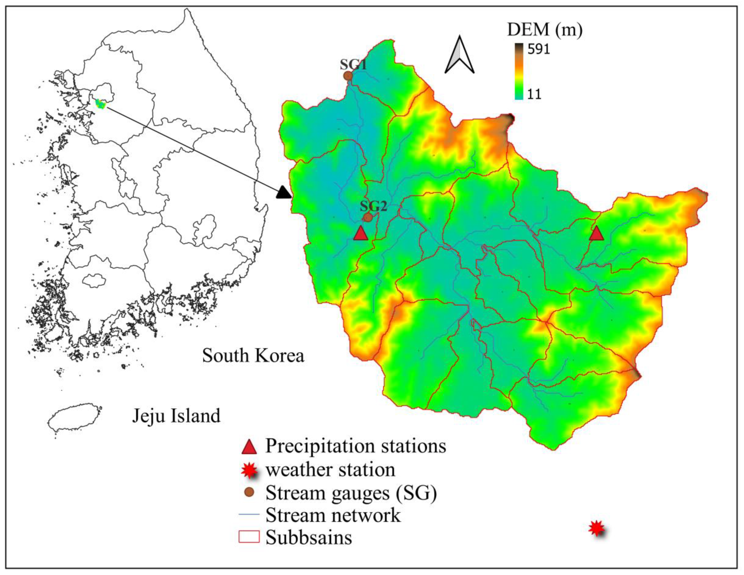
Figure 2.
Anyang watershed Land use and land cover (LULC) classes.
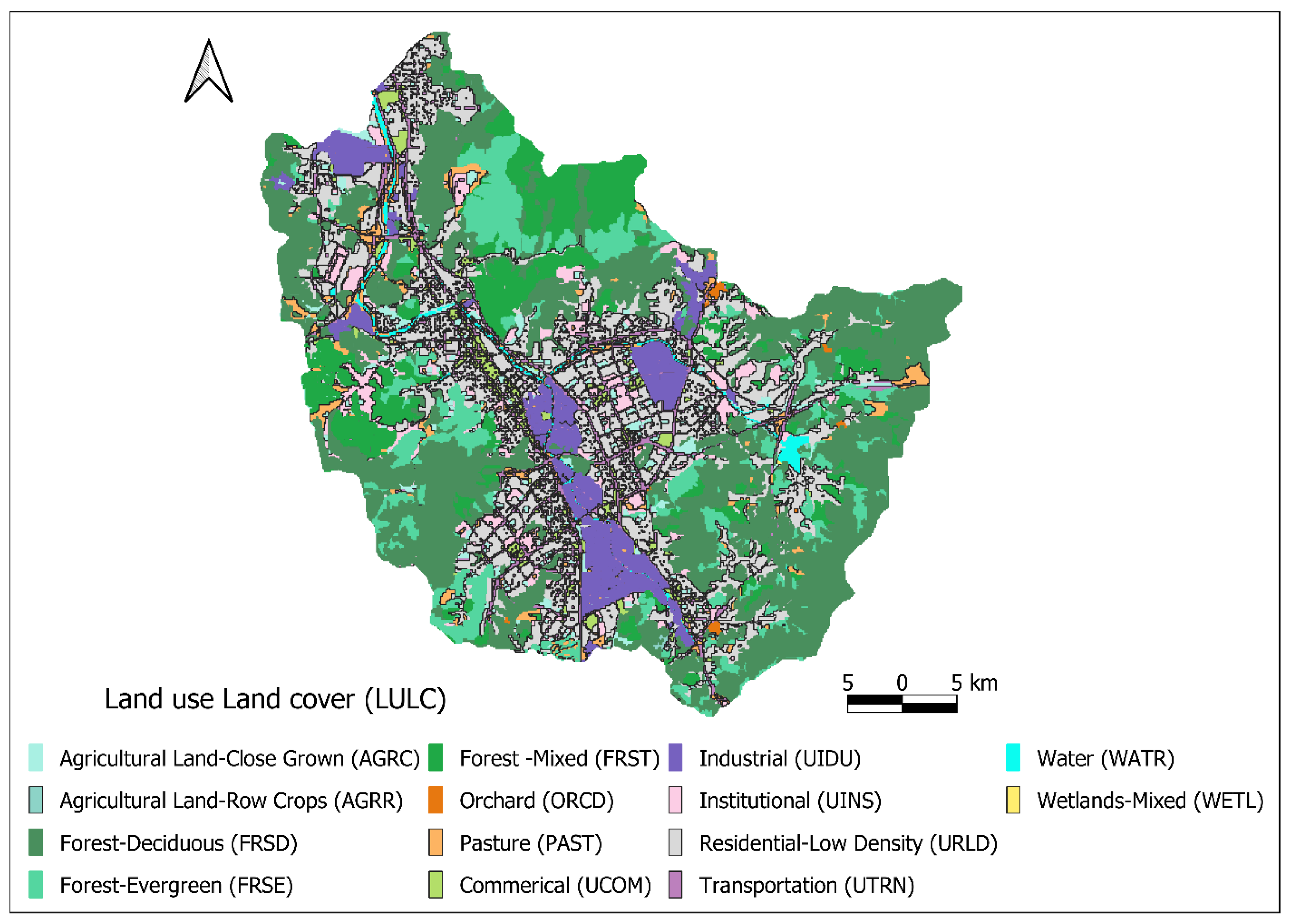
Figure 4.
Workflow of the SWAT-MODFLOW model and TWTFM. Adopted from Bailey et al. [41] for SWAT-MODFLOW and Chung et al. [59] for TWTFM method. .
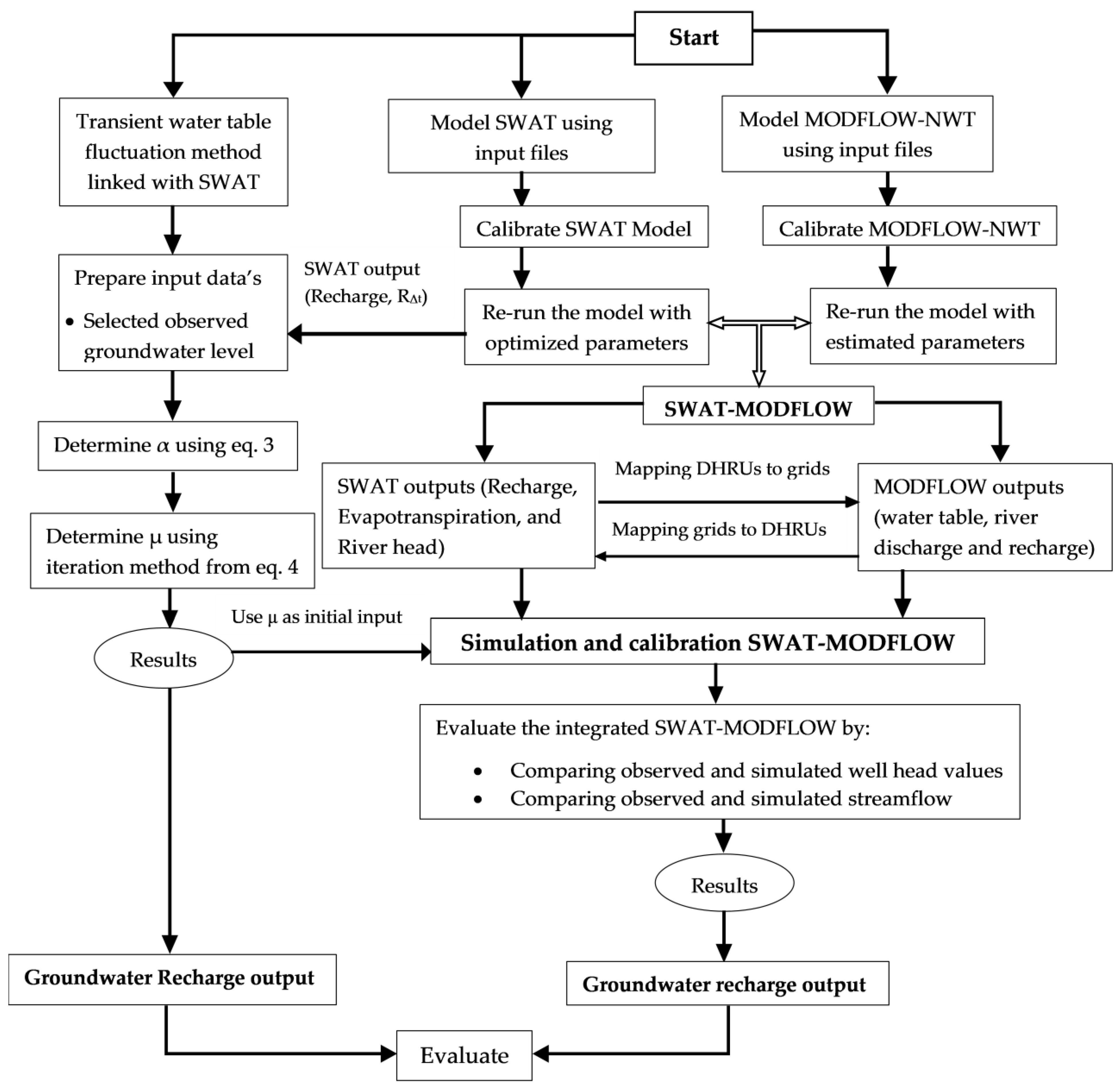
Figure 5.
Location of selected monitoring wells for TWTFM approach. .
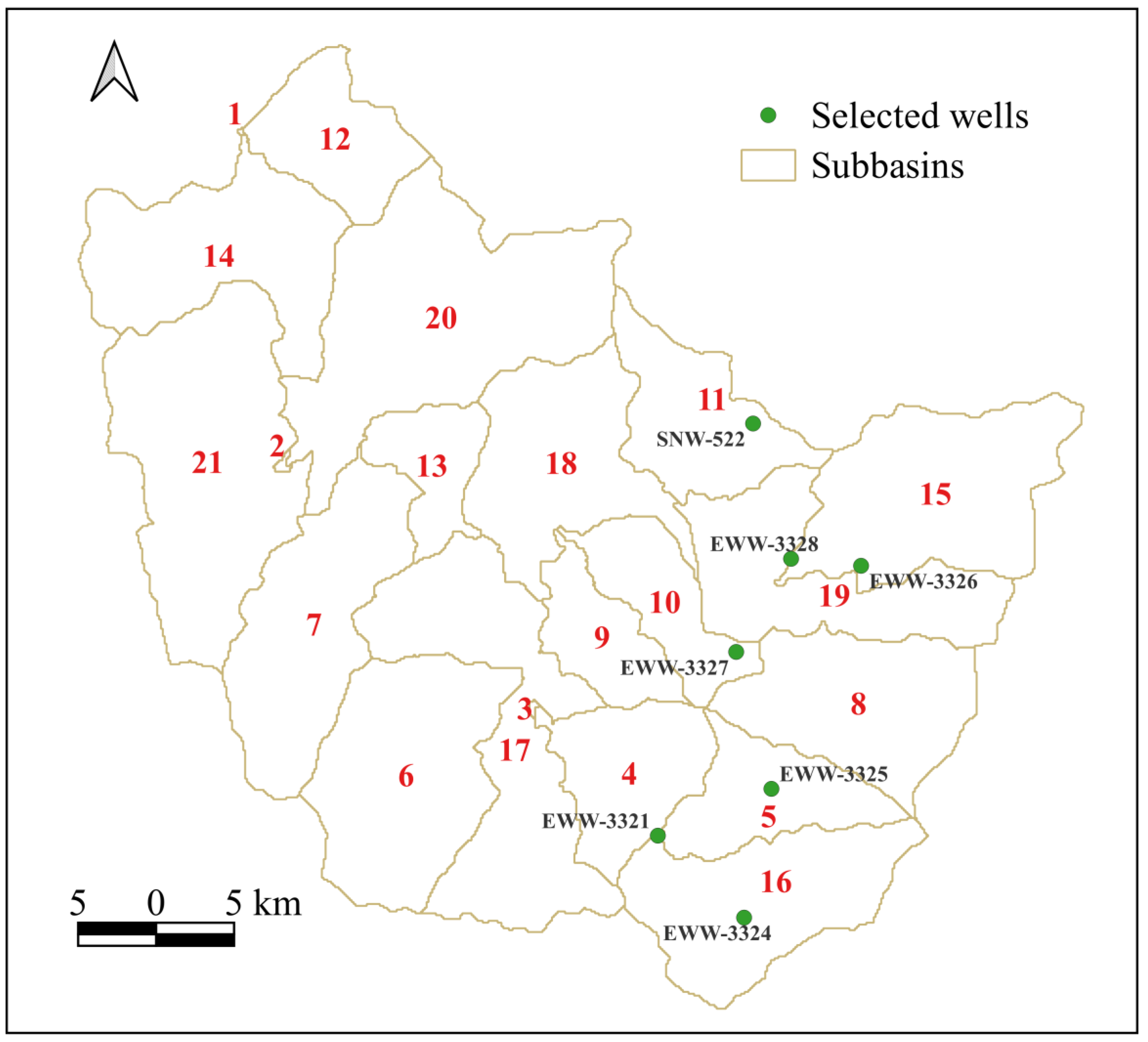
Figure 6.
Automated aquifer parameters distribution in study watershed.
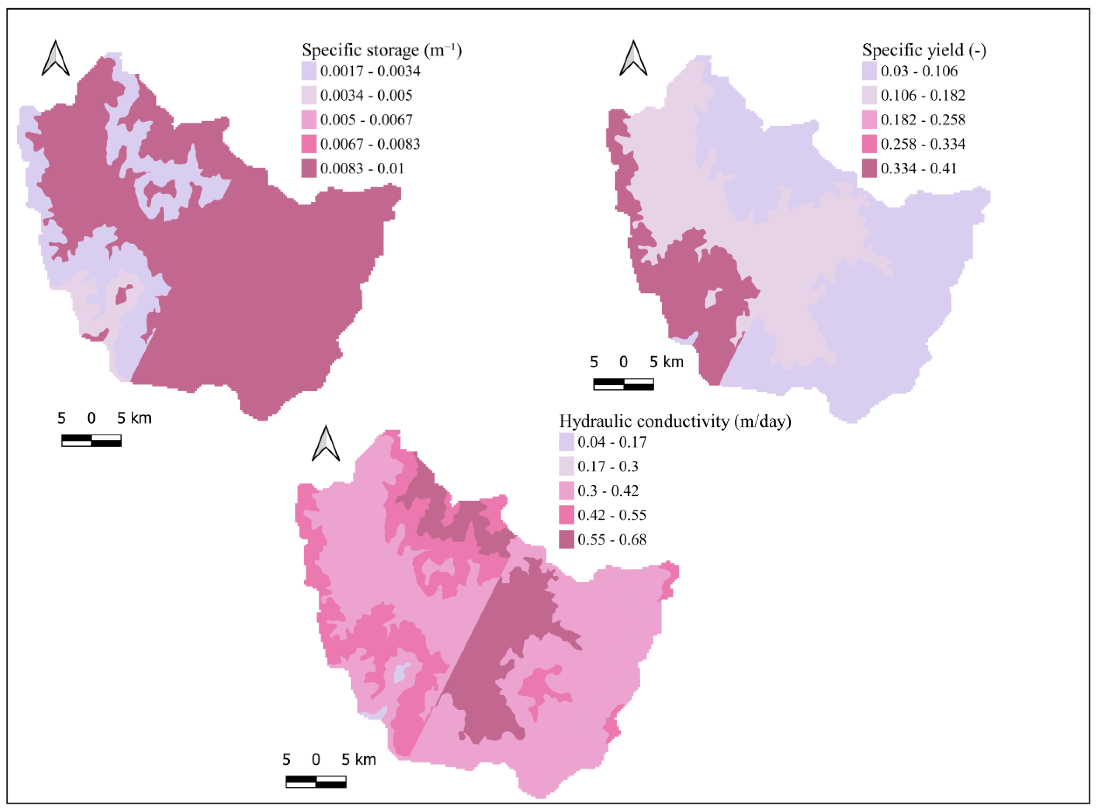
Figure 7.
Observed flow, simulated flow (SWAT (a) and SWAT-MODFLOW (b)), and precipitation at the stream station in the years 2009–2018.
Figure 7.
Observed flow, simulated flow (SWAT (a) and SWAT-MODFLOW (b)), and precipitation at the stream station in the years 2009–2018.
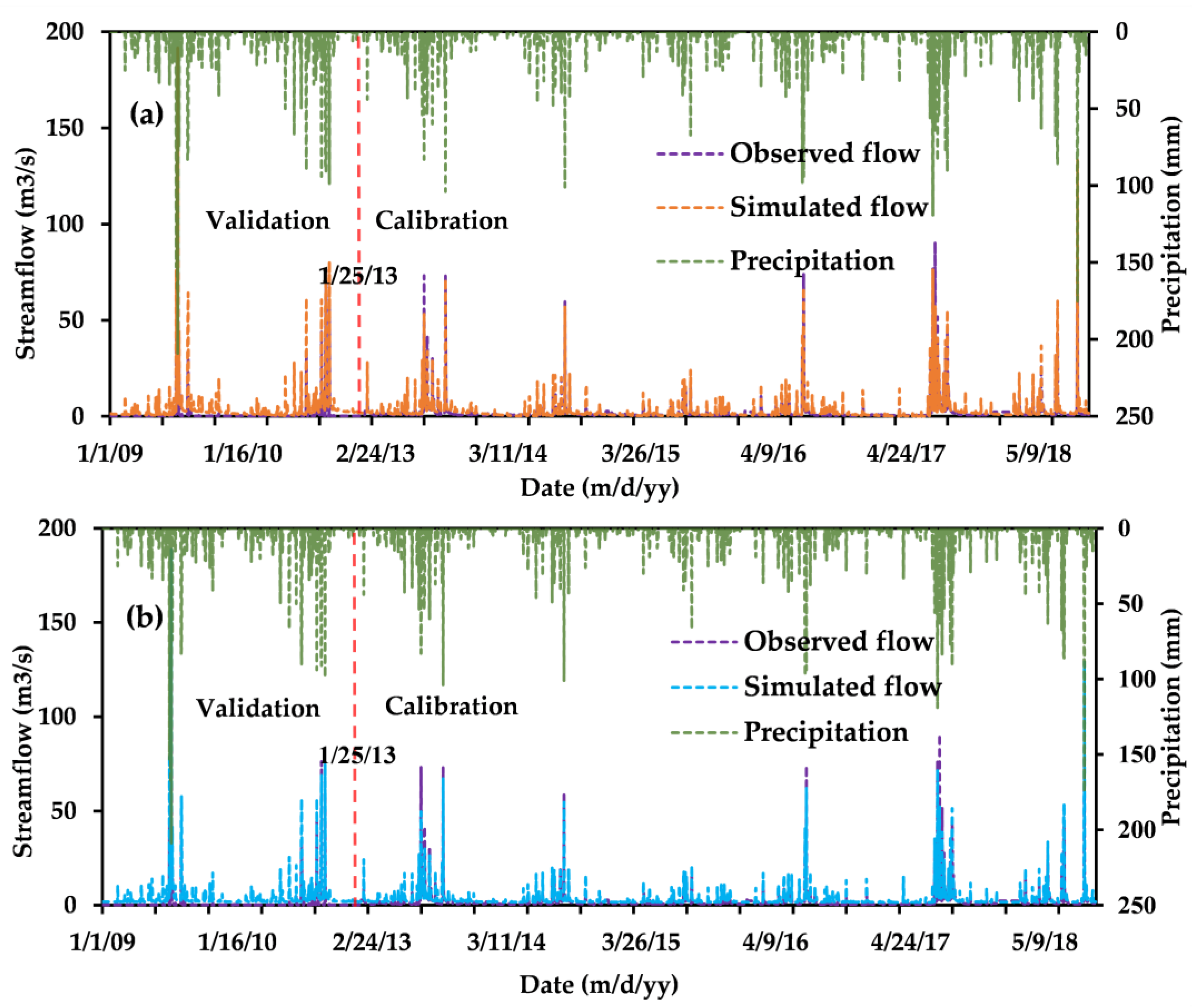
Figure 8.
Hydraulic head of the study region: (a) depth to water between observed and simulated (b) simulated hydraulic head from 2009–2018.
Figure 8.
Hydraulic head of the study region: (a) depth to water between observed and simulated (b) simulated hydraulic head from 2009–2018.
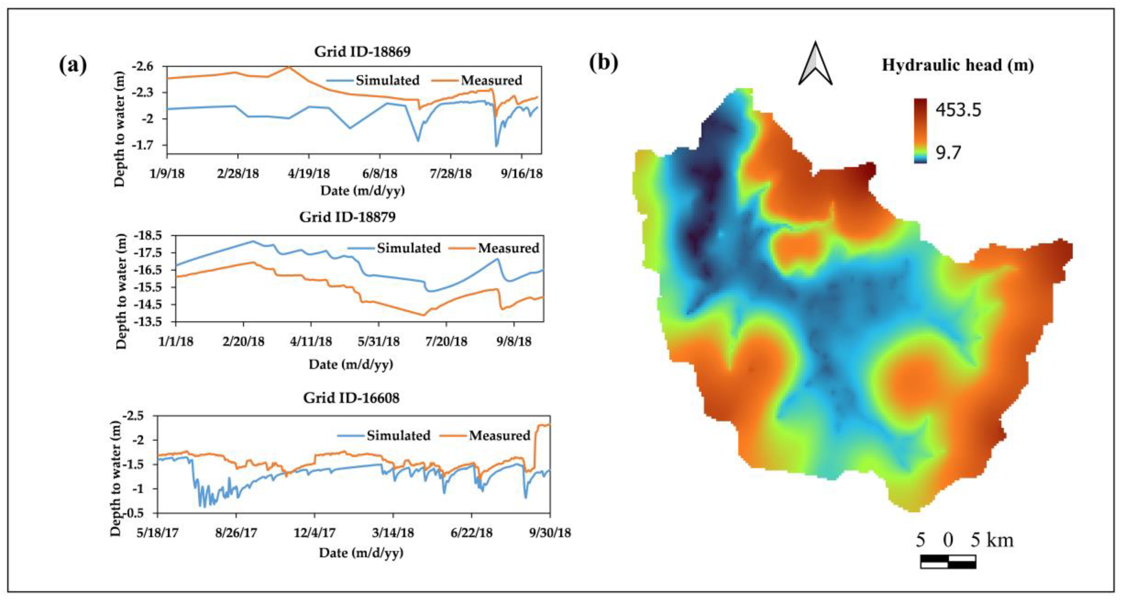
Figure 9.
Average groundwater recharge distribution from year 2009–2018: (a) monthly, (b) dry season, and (c) wet season.
Figure 9.
Average groundwater recharge distribution from year 2009–2018: (a) monthly, (b) dry season, and (c) wet season.
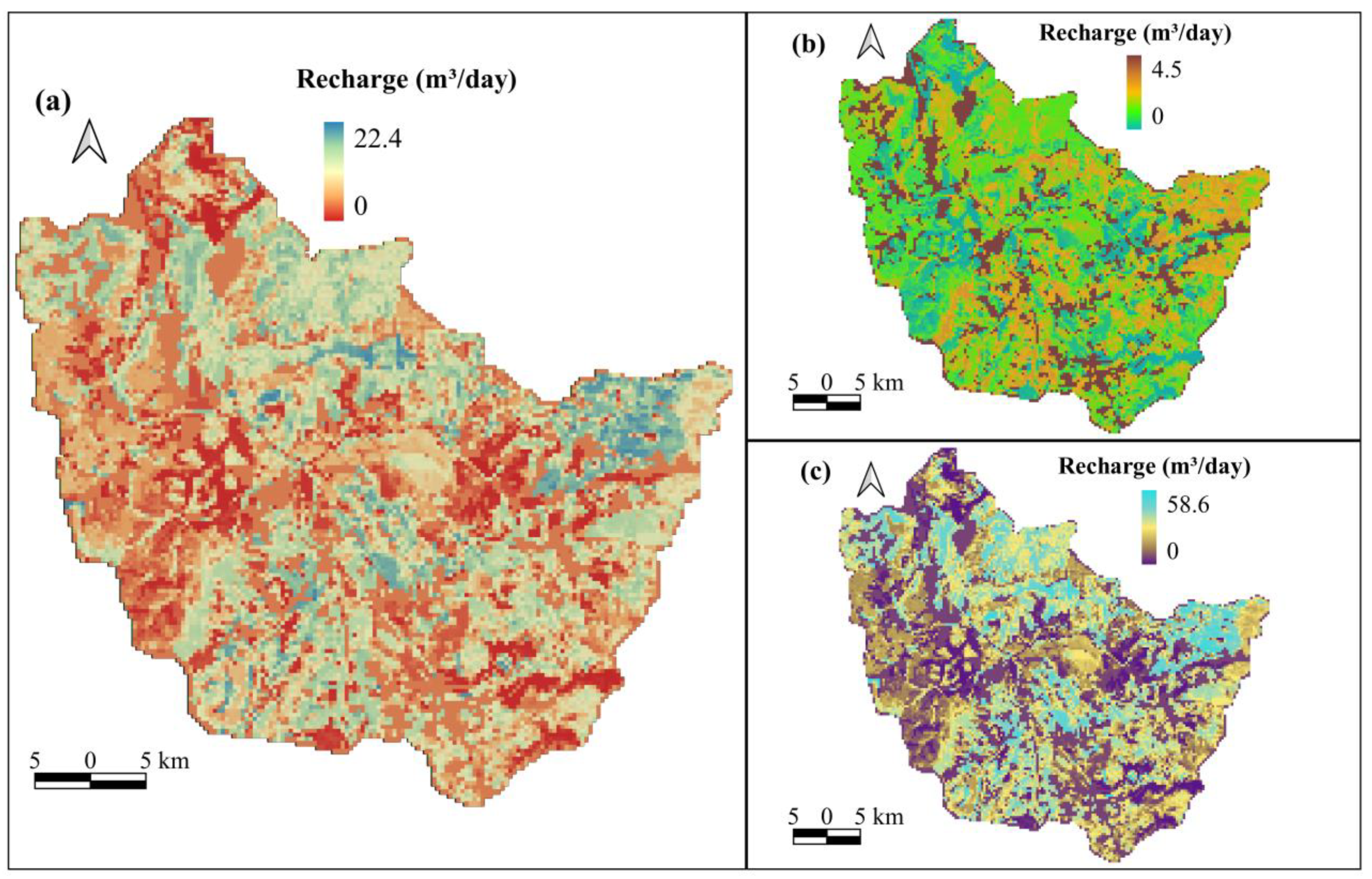
Figure 10.
SWAT-MODFLOW monthly water balance segments in the study region (mm) during year 2009–2018.
Figure 10.
SWAT-MODFLOW monthly water balance segments in the study region (mm) during year 2009–2018.
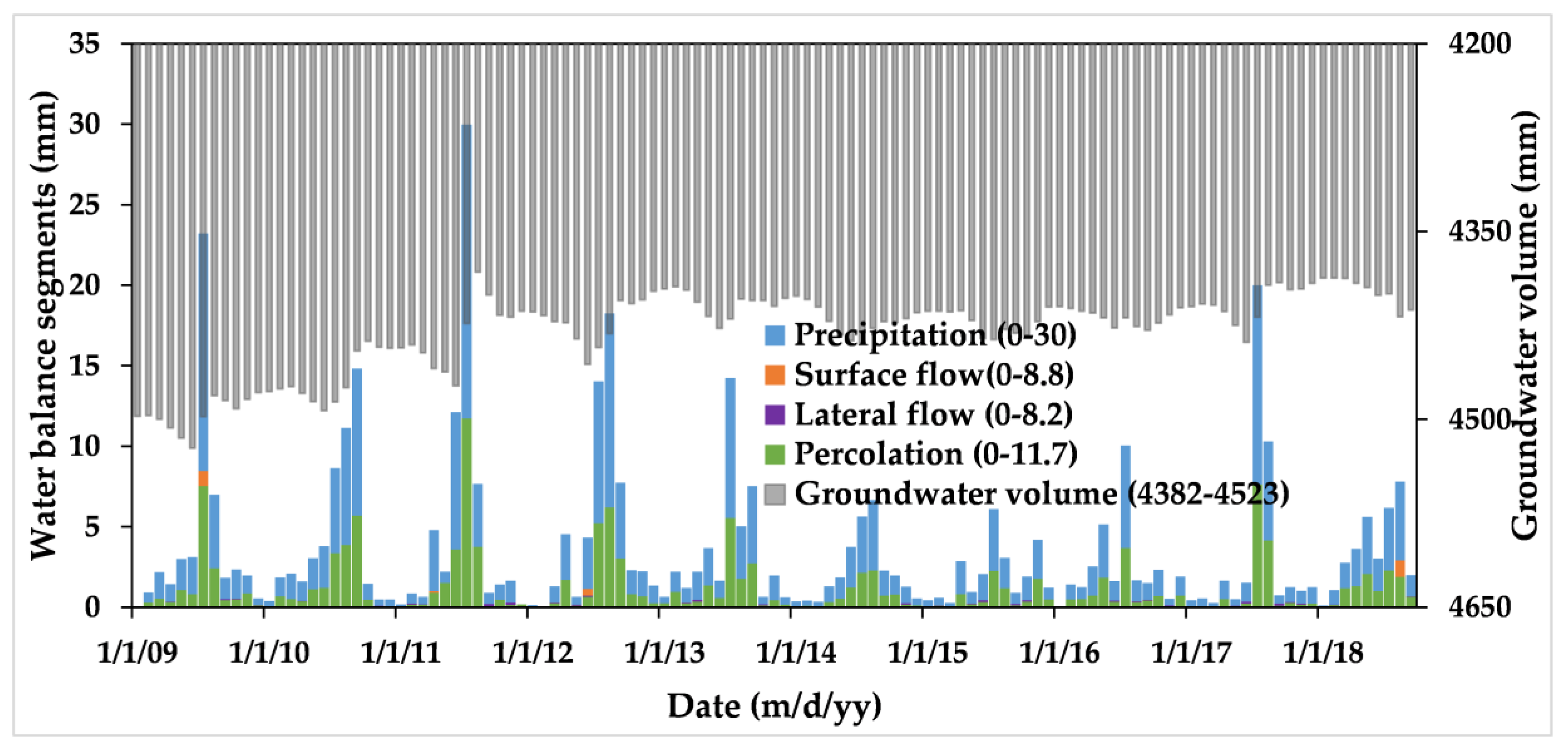

Table 1.
Description of SWAT model calibration parameters with fit and range values.
| Parameters | Description | Calibrated Value | Range Value |
| r_CN2.mgt | Initial SCS runoff curve no. for moisture condition II | 0.3 | 0.2-1.0 |
| v_ALPHA.BF.gw | Baseflow alpha factor (days) | 0.03 | 0.01-0.05 |
| v_GW_DELAY.gw | Groundwater delay (days) | 1 | 1-4 |
| v_GWQMN.gw | Threshold depth of water in the shallow aquifer for "revap" to occur (mm) | 530 | 460-1400 |
| v_GW_REVAP.gw | Groundwater "revap" coefficient | 0.05 | 0.01-0.09 |
| v_ESCO.hru | Soil evaporation compensation factor(-) | 0.3 | 0.15-0.5 |
| r_SOL_AWC.sol | Available water capacity of the soil layer (mm mm-1 ) | 0.03 | 0.01-0.05 |
| v_REVAPMN.gw | Threshold depth of water in the shallow aquifer for "revap" to occur (mm) | 430 | 187-450 |
| v_EPCO.hru | Plant uptake compensation factor(-) | 0.3 | 0.1-0.5 |
| v_RCHRG.gw | Deep aquifer percolation fraction | 0.3 | 0.05-0.4 |
r_ means original parameter is multiplied by (1+ a given value); v_ means replacing the existing parameter by a given value.
Table 2.
SWAT-MODFLOW selected calibration parameters descriptions and value ranges.
| Parameter | Value Range | Description |
| ALPHA_BF | 0.01-0.2 | Baseflow alpha factor (days),SWAT |
| CH_k2 | 1-50 | Main channel effective hydraulic conductivity (mm/h), SWAT |
| CN2 | 0.01-1 | Initial SCS runoff curve no. for moisture condition II, SWAT |
| EPCO | 0.1-1 | Plant uptake compensation factor(-), SWAT |
| ESCO | 0.1-1 | Soil evaporation compensation factor(-), SWAT |
| Hk | 0.01-100 | Hydraulic conductivity of aquifer (m/day), MODFLOW |
| Ss | 0.00001-0.01 | Specific storage (m-1), MODFLOW |
| Sy | 0.0001-0.4 | Specific yield (-), MODFLOW |
Table 3.
Final calibrated parameter value for SWAT-MODFLOW.
| Parameter | Calibrated Value | Description |
| ALPHA_BF | 0.01 | Baseflow alpha factor (days), SWAT |
| CH_k2 | 26 | Main channel effective hydraulic conductivity (mm/h), SWAT |
| CN2 | 0.08 | Initial SCS runoff curve no. for moisture condition II, SWAT |
| EPCO | 0.01 | Plant uptake compensation factor(-), SWAT |
| ESCO | 0.01 | Soil evaporation compensation factor(-), SWAT |
Table 4.
Summary of statistical parameters for SWAT and SWAT-MODFLOW performance during calibration and validation periods.
Table 4.
Summary of statistical parameters for SWAT and SWAT-MODFLOW performance during calibration and validation periods.
| Model | Calibration | Validation | ||
| R2 | NSE | R2 | NSE | |
| SWAT | 0.79 | 0.76 | 0.75 | 0.69 |
| SWAT-MODFLOW | 0.82 | 0.75 | 0.83 | 0.73 |
Table 5.
Estimated aquifer parameters and obtained recharge using TWTFM approach.
| Subbasins | Observed wells Name | Recharge (mm) (SWAT) | Recharge (mm) (TWTFM) | Specific yield (–) | Reaction factor (d-1) |
| 19 | EWW-3328 | 1001.2 | 994.4 | 0.017 | 0.2 |
| 16 | EWW-3324 | 1021.3 | 1020 | 0.022 | 0.04 |
| 15 | EWW-3326 | 806.2 | 806 | 0.01 | 0.12 |
| 11 | SNW-522 | 982.7 | 976.3 | 0.0078 | 0.2 |
| 10 | EWW-3327 | 702.5 | 702 | 0.0109 | 0.2 |
| 5 | EWW-3325 | 962.4 | 957.2 | 0.011 | 0.2 |
| 4 | EWW-3321 | 553.6 | 553.6 | 0.008 | 0.068 |
Disclaimer/Publisher’s Note: The statements, opinions and data contained in all publications are solely those of the individual author(s) and contributor(s) and not of MDPI and/or the editor(s). MDPI and/or the editor(s) disclaim responsibility for any injury to people or property resulting from any ideas, methods, instructions or products referred to in the content. |
© 2023 by the authors. Licensee MDPI, Basel, Switzerland. This article is an open access article distributed under the terms and conditions of the Creative Commons Attribution (CC BY) license (http://creativecommons.org/licenses/by/4.0/).
Copyright: This open access article is published under a Creative Commons CC BY 4.0 license, which permit the free download, distribution, and reuse, provided that the author and preprint are cited in any reuse.


