Submitted:
13 November 2023
Posted:
13 November 2023
You are already at the latest version
Abstract
Aim at a better understanding of the flow field around a fully appended Joubert BB2 submarine model and complementing the experimental investigations of the wake of the hydroplanes and sail, the Large eddy simulation (LES) with the dynamic Smagorinsky model is conducted. Three sets of grids with a maximum grid number of up to 228 million are designed, to perform the LES simulation for the Joubert BB2 at 10° yaw conditions, with a freestream Reynolds (Re) number based on the local freestream velocity and the hull length of ReL=2.2×10⁷. And comparison of the wake of the cruciform appendage is made with experiments, to verify the computational accuracy and examine the influence of the spatial resolution. A satisfactory result shows more favorable agreement with experimental measurements as the improvement of spatial resolution, with the relative error of the vortice centers well within 7.2% in the most refined grid arrangement. And under this grid arrangement, the evolution characteristics of three co-rotating vortices originating from the cruciform appendage are further described in detail at straight ahead and 10° yaw conditions.
Keywords:
Submarine
; LES
; Flow field
; Yaw
; Straight ahead
1. Introduction
The submarine will generate vortex structures with various scales and forms that develop downstream during navigation. Generalized appendages such as a sail, hydroplane, rudder, deck, and floodhole create coherent vortex structures, like the horseshoe vortex, tip vortex, Karman vortex, discrete vortex, et al., leading to intense flow vibration. The development of these vortex structures also influences the maneuverability and deteriorates the wake of the platform. The vortex oscillation and its induced pressure fluctuation excite the hull, resulting in flow-induced noise, which seriously influences the stealth. The investigation of the flow physics of a submarine can help to better understand maneuverability limitations and flow-induced noise sources.
A certain amount of available literature has described the flow around a submarine, among which experiment plays an important role, especially in early studies. Fu utilized a PIV (Particle image velocimetry) system to characterize the flow field around a sting-mounted captive ONR Body-1 submarine model in a steady turn (Fu et al., 2002). Jimenez and Ashok utilized a hot-wire system and a SPIV (Stereo particle image velocimetry) system to measure the flow field around an axisymmetric DARPA SUBOFF model, respectively, and the flow field experimental databases with different Reynolds numbers, pitch, and yaw angles were obtained (Jimenez et al., 2010; Ashok et al., 2012; 2013; 2014; 2015a; 2015b).
Another DSTO generic submarine model with a large deck, sail, and an X-form rudder arrangement (Joubert, 2004; 2006), which can provide a useful representation of a conventional submarine, has been widely discussed in the open literature. The flow field measurements of the fully appended model at both straight ahead conditions and during a 10° side-slip, were conducted by Defence Science and Technology (DST) Group, with data collected using pressure probes, PIV, and flow visualization of wool-tuft streamers (Kumar et al., 2012; Anderson et al., 2012; Jones et al., 2013; Lee et al., 2014; Manovski et al., 2014; Fureby et al., 2016). And it provided a benchmark prototype to validate and improve numerical simulations of submarine wakes.
Since a new vertical sail and two horizontal hydroplanes were designed to improve its stability and control characteristics (Bettle, 2014; Overpelt et al., 2015), which is known as “Joubert BB2” recently, the wind-tunnel experiment of the model at 10◦ yaw was conducted again, with China-clay visualization and a high-resolution SPIV system (Lee et al., 2018; 2019; 2020). And the wake of this cruciform appendage can be available to assist validation studies.
With the development of Computational Fluid Dynamic (CFD) methods, the numerical simulation of the flow field around a fully appended submarine model can complement the experimental investigations and create opportunities to advance the understanding of the flows, as the experiments only obtain limited flow field information. Careful verification and validation studies should be conducted with experimental data.
Three main CFD methods have been developed for predicting the flow field, and direct numerical simulation (DNS) is not practical in engineering prediction because of its enormous demand for computing resources, Reynolds Averaged Navier Stokes (RANS) and Large Eddy Simulation (LES) are gradually becoming dominant in computing the flow field around underwater vehicles. But for the fully appended hull, the RANS seems to slightly lack prediction accuracy, particularly for the second-order statistical moments and the local flow topology. The development of LES can provide very useful insights into the complicated transient nature of the flow, including unsteady wake flow, flow-induced noise, and vibrations (Bensow et al., 2006; Fureby et al., 2008; 2016; Toxopeus et al., 2012; Anderson et al., 2012; Zhang et al., 2016a).
The LES method was first proposed by Smagorinsky (Smagorinsky, 1963), and the applicability of predicting the flow field around submarines has been verified by many researchers. Alin and Bensow evaluated the predictive capabilities of LES by comparing it with experimental data from DTMB (Huang, 1992), and some generic features of the flow past DARPA SUBOFF configuration were discussed, both the fully appended model and the bare hull model. (Alin et al., 2003; 2010a; 2010b; Bensow, et al., 2004a; 2004b; 2006; 2008).
Anderson and Fureby performed LES computations of the fully appended DSTO generic submarine model at 10° yaw, and good qualitative agreement was found between the LES results and the experimental data, with respect to the velocity distributions and the locations of the main vortex structures (Anderson et al., 2012; Fureby et al., 2016). Norrison extends the computational studies by using a near-wall-modelled LES approach to simulate the flow around a full-scale, fully-appended Joubert generic submarine equipped with either a 5-bladed or 7-bladed propeller under straight-ahead (Norrison et al., 2016; 2017). The computational ability of LES for the surrounding flow of submarines under maneuvering conditions has been verified.
Zhang studied the numerical prediction approach for hydrodynamic force and noise of SUBOFF submarine appended by AU5-65 propeller by LES and Powell vortex theory (Powell, 1964), and expand LES to the field of submarine noise prediction and more complex maneuvering conditions, such as submarine propeller interaction and crashback (Zhang et al., 2010; 2014; 2016b; 2021; Wang and Zhang, 2022). The results further validated the numerical prediction ability of LES. Kroll performed LES of the flow over SUBOFF submarine appended by DTMB-4381 propeller in forward mode and crashback, mean flow fields and propeller load statistics show good agreement with experiments and previous simulations (Kroll et al., 2020).
In the paper, three sets of grids with a maximum grid number of up to 228 million are designed, to perform the LES simulation for the fully appended Joubert BB2 submarine model at 10° yaw. And a comparison of the wake of the sail and hydroplanes is made with Lee’s work (Lee et al., 2019), to verify the grid convergence and computational accuracy of LES in terms of predicting the flow field around the submarine. Simulations are conducted at a freestream Reynolds (Re) number based on the local freestream velocity and the hull length of ReL=2.2×10⁷, which is higher than those in previous work and more representative of a full-scale submarine. Then the characteristics of the flow around the submarine are described in detail at straight ahead and 10° yaw conditions. These computations further elucidate the structure of the flow around the fully appended Joubert BB2 submarine model, and provide an effective complement to the experimental investigations.
2. The Joubert BB2 Submarine Model
Figure 1 shows the Joubert BB2 submarine model with a length L=3.826 m and a model scale of 1:18.348. The hull is designed as an axisymmetric body of revolution with a length-to-diameter ratio L/2rm = 7.3, and the bow profile is derived from a NACA0018 curve (Loid and Bystrom, 1983), splined to allow the rise in pressure to occur further aft (Fureby et al., 2016). The cross-section of the sail is based on a NACA0022 with a height of 0.080L and a chord length of 0.157L. Two horizontal NACA0015 hydroplanes are assembled on the sail, and the combined span and the root chord are designed as 0.117L and 0.033L respectively. The stern control plane consists of four rudders in an X configuration, and the tailing edge is 0.075L away from the end of the hull. A further detailed description can be found in Joubert (Joubert, 2006), Bettle (Bettle, 2014), and Overpelt (Overpelt et al., 2015).
In Lee’s work (Lee et al., 2019), the experimental results are discussed in a wind axis coordinate system, with the x-axis direction defined as the direction of freestream as shown in Figure 2, which is also adopted in the paper for more direct comparison. The velocity field is obtained with a SPIV measurement system at three selected model-length locations x/L=0.511, x/L=0.650, and x/L=0.815, and the normal direction of these experimental planes is parallel to the free-stream direction. For further details on SPIV setup and measurements, see Lee (Lee et al., 2019). It should be noted that the model-length Reynolds numbers are chosen as ReL=4×10⁶ and ReL=8×10⁶ in the experiments, which are lower than those of this paper. The conclusion has been drawn that it shows similar experimental results of the velocity field, turbulence kinetic energy (TKE), cross-stream Reynolds stress, and et al. under different ReL, and according to previous research results on the wake field of submarines models, when the ReL increases from 1×10⁷ to 3.5×10⁷, the dimensionless mean velocity changes between 3% and 10%, the reciprocal validation of computations and experiments is still reliable.
3. Numerical Methodology
3.1. Large Eddy Simulation
The commercial CFD code StarCCM+ by Siemens PLM based on the finite volume method is utilized to conduct the LES simulations presented in the paper. For LES, large scales by which transport is largely governed are directly computationally resolved by the spatially filtered Navier-Stokes equations, and small scales are modeled by appropriate subgrid-scale turbulence models. The vortex flow is separated into small and large eddies, achieved by means of a low-pass filter. The filtered Navier-Stokes equations are as follows:
Where is the denity, is the filtered velocity, is the filtered pressure, is the identity tensor, and is the resultant of the body forces. is the filtered stress tensor due to molecular viscosity and is the subgrid-scale stress, where is the strain rate tensor and computed from the resolved velocity field . To model the sub-grid-scale stress terms, the dynamic Smagorinsky model proposed by Germano (Germano et al., 1991) and modified by Lilly (Lilly et al., 1992) is used here. This approach has shown good performance for a variety of complex marine flows of full appended submarines (Zhang et al., 2010; 2016b; 2021; Mahesh et al., 2017; Kumar et al., 2018; Kroll et al., 2020; Wang and Zhang, 2022).
As for the discretization of the governing equations, a bounded central difference scheme is applied. The coupling between the velocity and pressure is achieved by means of the classic PISO algorithm, and the algebraic multigrid method is employed to accelerate the solution convergence.
3.2. Computational Domain and Boundary Condition
Figure 3 shows the cylindrical computational domain, the domain has a length of 4L and a radius of L, and extends from L upstream of the front of the hull to 2L downstream of the stern of the hull, for modeling a fully developed wake. Free-stream boundary conditions are imposed at the inflow and radial boundaries, and a pressure-outlet boundary condition is imposed at the outflow boundary. The no-slip wall treatment is used for shear stress specification.
3.3. Computation Mesh
In this subsection, three sets of grids are designed for convergence study. The simulation domain is discretized using the unstructured hex-dominant grid (trimmer mesher, Octree grid), and a prism layer mesher is used for the generation of boundary layer mesh with y+ ≈ 1 for all grid sets. The refinement ratio of grids in three directions is , as recommended by the International Towing Tank Conference (ITTC, 2014). The corresponding grid numbers are 3.30 × 10⁷, 8.62 × 10⁷, and 2.28 × 10⁸ respectively and the three grid codes are G1 to G3 respectively. All numerical simulations are carried out by parallel processing in CSSRC (China Ship Scientific Research Centre) with 50 nodes (2400 processors). The time needed to finish a simulation with 228 million cells is about 30 days.
For capturing the flow field more accurately, a local volumetric control block is established around the submarine to control the surrounding grid size. Care is taken to resolve initial vortex formation and roll up of the free shear layer, and avoid rapid dissipation of vortex structure in the wake of the sail, hydroplanes, and X-rudder, local volumetric control blocks are also established around these appendages for more refined volume mesh control. There is an angle of approximately 5.5 degrees between the blocks and the longitudinal axis of the hull in calculation at 10°yaw conditions.
4. Results and Discussion
In this section, we present results initially for the qualitative and quantitative comparison between the numerical results and experimental results at 10° yaw, and then the detailed numerical investigation of the flow around the submarine is conducted at straight ahead and 10° yaw conditions.
4.1. Validation of the Numerical Approach
Figure 5 provides a direct comparison of the wake of the cruciform appendage, including the mean resultant velocity , the vertical component of velocity , and the cross−stream Reynolds stress , where denotes the freestream velocity. The experimental results with ReL= 4 × 10⁶ and ReL= 8 × 10⁶ are denoted by Exp. 1 and Exp. 2 respectively. It can be observed that the sail-tip vortex formed by the rolling up of the wake can be presented by the numerical calculations under all sets of girds. The region of the core flow, defined as a region of vortex flow from its center to its radial location of maximum swirl, is quite similar to the experimental results. While the range of the core flow and low-velocity region presents minor differences under different sets of grids. Especially for the vertical component of velocity, as the number of grids increases, the distribution of high/low-velocity regions becomes more concentrated and obvious, and the numerical results are closer to the experiments. In addition, the numerical dissipation decreases as the grid number increases, and the capture of the cross-stream Reynolds stress seems to be more refined.
Figure 6 shows a comparison of the mean resultant velocity as functions of radial distance ry/L from the vortex center, in the horizontal profiles through the sail-tip vortex. The mean resultant velocity under different grid sets exhibits a considerable difference, especially for the region of the core flow, which presents a corresponding increase with the grid number’s continuous growth. The core-flow velocity obtained from numerical calculations exhibits a significant difference at different axial distances from the bow, but is quite close for the experiments. The core flow obtained in the first set of grids (G1) has a mean velocity and at x/L=0.511 and x/L=0.815 respectively, with an axial descent rate of 18.8%. It corresponds to and respectively in G3, with an axial descent rate of 11.9%. It indicates that the numerical attenuation inevitably exits in the LES simulations with the dynamic Smagorinsky model of the core flow, which is not advantageous compared to experiments, and can be partly eliminated by improvement of the spatial resolution of the grid.
Figure 7 shows a comparison of the vertical component of velocity . It can be seen that the numerical results become gradually closer to the experimental values as the grid number increases. Especially for the prediction of the peak and valley values, the results obtained in G3 are quite close to that of Exp. 2 with a relatively higher Reynolds number. Overall, the relative errors of the peak and valley values in G3 are 10.6% and 4.3% respectively, which turns to 13.2% and 14.0% in G2, and 21.6% and 21.1% in G1. It can be concluded that with the refinement of the grids, the extreme values can be more accurately captured in numerical simulations, due to the improvement of spatial resolution.
Figure 8 provides a plot of the comparison of the turbulence kinetic energy (TKE) for the sail-tip vortex. The distribution of TKE along the radial distance ry/L for all grid sets is consistent with the experimental results, and the simulations of G3 are more representative of the experiments, with the relative error of the peak value in the region of core flow being relatively smaller.
Figure 9 summarizes the comparison of the centerline of the sail wake, which is defined by tracing the boundary <uxuy > = 0 between the positive and the negative Reynolds stresses. Overall, the sail-wake centerline shifts very slightly windward by no more than 0.01L, and by refining the grids from G1 to G3, it shifts leeward and closer to the experiments. The centers of the vortices on the upper hull are listed in Table 1, and their relative errors to Exp. 2 are listed in Table 2. In the near sail-wake region (x/L=0.511), the numerical simulations for all grid sets can well define the centers of the vortices, but as they evolve downstream, the advantages of refining the grids are gradually being reflected. For the case of G3, the maximum horizontal and vertical relative errors of the vortice centers at x/L=0.815 are 7.2% and 1.5%, which is quite satisfied with actual engineering predicting needs.
4.2. Analysis of the Evolution of the Flow
Figure 10 presents an overall view of the flow past Joubert BB2 at straight ahead conditions in terms of the second invariant of the velocity gradient Q, colored by the mean resultant velocity . In the immediate front of the junctions of the sail root and the deck, the flow rolls up into a horseshoe vortex system surrounding the sail, the legs of which develop downstream following the deck. Because of the adverse pressure gradient at the trailing edge of the sail, the flow gradually develops into turbulence, and the side vortices are formed and interact with the horseshoe vortex at the root. The side vortices over the sail cap are transported along the sail edge, then merge with the sail-tip vortices and dissipate rapidly. The flow over the outer edge of the hydroplanes induces a pair of hydroplane-tip vortices with opposite circulation, which develop downstream independently, then dissipate and disappear at a distance of approximately one submarine length from the stern. Further, horseshoe vortex, tip vortex, and wake vortex systems can be observed around the X-rudders. And between the two upper rudders, they interact with the vortices sweeping down and sideways over the end of the deck, complicating the flow into the propeller disk, which is unstable and the main source of propeller hydrodynamic noise. Downstream far away from the hull, all the tip vortices dissipate and almost only the wake vortices after complicated interaction dynamically evolve with the energy gradually weakening.
Similarly, Figure 11 presents various vortex systems past Joubert BB2 at 10° yaw conditions, from perspectives of oblique, top, and side views. It can be clearly seen that the vortex systems are more complicated. The side vortices on the leeward side of the sail occur more forward, and the sail-tip vortices are relatively strong enough to develop far downstream. The same as the hydroplane-tip vortices, but which are not clearly observed downstream because of strong interaction with the sail wake. Figure 12 shows the development of the trajectories of the cores of tip vortices originating from the cruciform appendage, including the port and starboard hydroplanes and the vertical sail, at 10° yaw conditions. The clockwise rotating sail-tip vortices maintain an axial angle of approximately 8 degrees with the hull and develop downstream and leeward, and are almost stable vertically after experiencing a brief down-wash immediately behind the sail. The position of the port hydroplane-tip vortices fluctuates widely, the horizontal and vertical coordinates of which reach their maximum values approximately at x/L=1.1 and x/L=0.7 respectively, then experience a sharp drop. Overall, the port hydroplane-tip vortices develop and revolve around the sail-tip vortices. The development of the starboard hydroplane-tip vortices is relatively stable, whose core keeps moving towards the leeward side, with the vertical position gradually rising away from the hull after passing through a valley approximately at x/L=1.1, due to the repulsive interaction of the hull wake.
At 10° yaw conditions, another obvious feature that distinguishes the straight ahead conditions is the flow separation on the leeward side of the middle hull. The upper and lower vortex system can be clearly seen, and the former eventually interacts with the horseshoe vortex system originating from the sail, while the latter merges into the wake between the upper and lower rudders. The wake of the submarine becomes quite complicated, and the flow behind the stern is dominated by the mixing of various component vortex systems, including the tilted horseshoe vortex system, the upper and lower hull vortices, the tip vortices, and the wake of the sail, hydroplanes, X-rudders, and hull.
Figure 13 shows the evolution of the mean vorticity magnitude along the submarine axial, at straight ahead and 10° yaw conditions, where .The momentum and energy are transported by the development of vortex systems, where the vortex systems generated by the sail, hydroplanes, deck, hull, and X-rudder pass present an increase in vorticity, especially for the tip vortices, horseshoe vortices, wake vortices, and generated hull side vortices possibly. Noticing that the instabilities of the horseshoe-vortex system and its interaction with the hull boundary layer, cause the legs to break up and develop connected vortex loops, which results in the transport of momentum across the hull and influences the distribution of the vorticity, as mentioned by Fureby (Fureby et al., 2016). As the vortex structure gradually dissipates downstream, the vorticity gradually decreases, with the sail-tip vortices and hydroplane-tip vortices being particularly prominent. For the case straight ahead, the obvious vorticity near the sail induced by the tip vortices of the cruciform appendage quickly decays, which is quite significantly far away from the stern for the case at 10° yaw. Increased vorticity is also found around and behind the hull at 10° yaw conditions because of considerable interaction between the flow and the hull. Therefore, the flow-induced noise of submarines under maneuvering conditions has always been a research highlight in the international hydrodynamics field. As the vortex systems develop from a concentrated distribution in the near wake region to a dispersed mode in the far field in both cases, the vorticity gradually weakens while the coverage range increases, due to energy conservation.
Figure 14 shows the evolution of the turbulence kinetic energy (TKE) along the submarine axial, at straight ahead and 10° yaw conditions. The evolution of TKE is quite similar to that of the mean vorticity magnitude, where the vorticity is concentrated, the momentum is intense and the TKE is significant. For the case at 10° yaw, it can be obviously seen that the TKE induced by the sail-tip vortices is quite stronger than that induced by the hydroplane-tip, with the same pattern as the vorticity followed. Besides that, the TKE in the wake is strongly influenced by the X-rudder at both conditions, which exacerbates the velocity fluctuations of the flow and induces additional propeller noise, thus the hydrodynamic design of the X-rudder is also a research highlight.
Figure 15, Figure 16, and Figure 17 show a comparison of the mean resultant velocity , the mean vorticity magnitude , and the turbulence kinetic energy respectively, for the model-length locations x/L=0.484, at straight ahead and 10° yaw conditions. A pair of sail-tip vortices with opposite circulation can be found at straight ahead conditions, and in the core-flow region, the mean resultant velocity, the mean vorticity magnitude, and the turbulence kinetic energy are quite smaller than those at 10° yaw conditions.
In view that the momentum and energy transported by the sail-tip vortices at 10° yaw conditions are quite predominant, the flow characteristics of the sail-tip vortices are further studied below. Figure 18 provides a comparison of the velocity for the sail-tip vortex under different longitudinal locations, including mean resultant velocity , the three-dimensional component of velocity , and . It can be intuitively seen that as the wake of the sail-tip vortices develops downstream, the mean resultant velocity, streamwise velocity, and horizontal velocity show a gradually decreasing trend, and the fluctuation of the vertical velocity between peak and valley values gradually weakens. In the near wake region where x/L≤0.807, the core flow exhibits a high-velocity characteristic, while in the far wake region, the velocity is smaller than the freestream velocity.
Figure 19 shows a comparison of the mean vorticity under different streamwise locations. The dominant component of the mean vorticity magnitude is the streamwise mean vorticity , which indicates that the sail-tip vortex rotates rather faster around the x-axis compared to the other two. The core-flow vorticity weakens rapidly as the wake develops downstream, while the decay rate gradually slows down. An interesting phenomenon shows that the distribution of the peaks and valleys of the vertical mean vorticity changes with the evolution of the flow. In the near wake region where x/L≤0.807, the peaks are located on the windward side, and the valleys are located on the leeward side, while in the far wake region, the positions of the two are exactly opposite.
Figure 20 shows a comparison of the turbulence kinetic energy under different streamwise locations. The roll-up from the sail is accompanied by a down-wash of the sail-tip vortex (see Figure 12(a)), and the normal stress in the vertical component <uxux> is the strongest contribution to the TKE, as mentioned by Lee (Lee et al., 2019). Because of the significant cross-stream, the normal stress in the horizontal component accounts for the second strongest contribution, and the normal stress in the streamwise component is the weakest. The strongest TKE does not occur immediately behind the sail, but approximately in the range of x/L equal to 0.6 to 1.0, where the down-wash of the sail-tip vortex is quite intense.
5. Conclusions
In the paper, the large eddy simulation with the dynamic Smagorinsky model is conducted, to investigate the flow field around a fully appended Joubert BB2 submarine model at straight ahead and 10° yaw conditions. Conclusions acquired from the analysis of computed results can be summarized as:
- 1)
- By qualitative and quantitative comparison with experiments at 10° yaw conditions, the computational accuracy is verified. A satisfactory result shows more favorable agreement with experimental measurements as the improvement of spatial resolution, especially for capturing the vortice centers in the far wake region, with the relative error well within 7.2% in the most refined grid arrangement.
- 2)
- The resultant velocity, vorticity magnitude, and TKE show a gradually decreasing trend as the wake of the cruciform appendage develops downstream. At 10° yaw conditions, the core flow velocity of the sail-tip vortices will transition from high-velocity characteristics in the near wake region, to low-velocity characteristics as the wake further evolutions.
- 3)
- The tip vortex tracking at 10°yaw conditions exhibits significant three-dimensional characteristics than that at straight ahead conditions. In the core-flow region, the resultant velocity, vorticity magnitude, and TKE at straight ahead conditions are quite smaller than those at 10° yaw conditions.
- 4)
- At 10° yaw conditions, the sail-tip vortex tracking maintains an axial angle of approximately 8 degrees with the hull, and is almost stable vertically after experiencing a down-wash immediately behind the sail. The port hydroplane-tip vortices develop and spiral around the sail-tip vortices, while the core of the starboard hydroplane-tip vortices keeps moving towards the leeward side, with the vertical position gradually rising away from the hull after passing through a valley approximately at x/L=1.1, due to the repulsive interaction of the hull wake.
Funding
Support from the projects with the Grant No. 50907010101 is acknowledged.
CRediT Authorship Contribution Statement
Mo Chen: Conceptualization, Methodology, Software, Writing -original draft. Nan Zhang: Conceptualization, Methodology, Data curation, Validation, Supervision. Hailang Sun: Visualization & Investigation. Xuan Zhang: Writing-review & editing.
Data Availability Statement
The data that has been used is confidential.
Conflicts of Interest
The authors declare that they have no known competing financial interests or personal relationships that could have appeared to influence the work reported in this paper.
References
- Alin, N.; Fureby, C. LES of the flow past simplified submarine hulls. In Proceedings of the 8th International Conference on Numerical Ship Hydrodynamics, Busan, Korea; 2003. [Google Scholar]
- Alin, N.; Bensow, R.; Fureby, C.; et al. Current capabilities of RANS, DES and LES for submarine flow simulations. J. Ship. Res. 2010, 54, 184–196. [Google Scholar] [CrossRef]
- Alin, N.; Chapuis, M.; Fureby, C.; et al. Numerical study of submarine propeller-hull interactions. In Proceedings of the 28th Symposium on Naval Hydrodynamics, Pasadena, USA; 2010. [Google Scholar]
- Anderson, B.; Chapuis, M.; Erm, L.; et al. Experimental and computational investigation of a generic conventional submarine hull form. In Proceedings of the 29th Symposium on Naval Hydrodynamics, Gothenburg, Sweden; 2012. [Google Scholar]
- Ashok, A.; Smits, A.J. The turbulent wake of a submarine model at varying pitch and yaw angle. In Proceedings of the 65th Annual Meeting of the APS Division of Fluid Dynamics, San Diego, California; 2012. [Google Scholar]
- Ashok, A.; Smits, A.J. The turbulent wake of a submarine model in pitch and yaw. In Proceedings of the 51st AIAA Aerospace Sciences Meeting including the New Horizons Forum and Aerospace Exposition, Grapevine, Texas; 2013. [Google Scholar]
- Ashok, A.; Buren, T.V.; Smits, A.J. Asymmetries in the high Reynolds number wake of a submarine model in pitch. In Proceedings of the 67th Annual Meeting of the APS Division of Fluid Dynamics, San Francisco, California; 2014. [Google Scholar]
- Ashok, A.; Buren, T.V.; Smits, A.J. The structure of the wake generated by a submarine model in yaw. Exp. Fluids 2015, 56, 123. [Google Scholar] [CrossRef]
- Ashok, A.; Buren, T.V.; Smits, A.J. Asymmetries in the wake of a submarine model in pitch. J. Fluid Mech. 2015, 774, 416–442. [Google Scholar] [CrossRef]
- Bensow, R.E.; Fureby, C.; Liefvendahl, M.; Persson, T. A comparative study of RANS, DES and LES. 26th Symposium on Naval Hydrodynamics, Rome, Italy; 2004. [Google Scholar]
- Bensow, R.E.; Persson, T.; Fureby, C.; et al. Large eddy simulation of the viscous flow around submarine hulls. In Proceedings of the 25th Symposium on Naval Hydrodynamics, Newfoundland and Labrador, Canada; 2004.
- Bensow, R.E.; larson, M.G. Towards a novel residual based subgrid modelling based on multiscale techniques. In Proceedings of the 9th Numerical Towing Tank Symposium, Le Croisic, France; 2006. [Google Scholar]
- Bensow, R.E.; Liefvendahl, M. Implicit and explicit subgrid modeling in LES applied to a marine propeller. In Proceedings of the 38th Fluid Dynamics Conference and Exhibit, Seattle, Washington; 2008. [Google Scholar]
- Bettle, M.C. Validating design methods for sizing submarine tailfns. In Proceedings of the Warship 2014: naval submarines and UUV’s, Bath, UK; 2014. [Google Scholar]
- Fu, T.C.; Atsavapranee, P.; Hess, D.E. PIV measurements of the cross-flow wake of a turning submarine model (ONR Body-1). In Proceedings of the 24th Symposium on Naval Hydrodynamics, Fukuoka, Japan; 2002. [Google Scholar]
- Fureby, C. Large eddy simulation of ship hydrodynamics. In Proceedings of the 27th Symposium on Naval Hydrodynamics, Seoul, Korea. 2008. [Google Scholar]
- Fureby, C.; Anderson, B.; Clarke, D.; et al. Experimental and numerical study of a generic conventional submarine at 10° yaw. Ocean Eng. 2016, 116, 1–20. [Google Scholar] [CrossRef]
- Germano, M.; Piomelli, U.; Moin, P.; Cabot, W. A dynamic subgrid-scale eddy viscosity model. Physics of Fluids A 1991, 3, 1760–1765. [Google Scholar] [CrossRef]
- Huang, T.; Liu, H.L.; Groves, N.; et al. Measurements of flows over an axisymmetric body with various appendages: the DARPA SUBOFF experiments program. In Proceedings of the 19th Symposium on Naval Hydrodynamics, Seoul, Korea; 1992. [Google Scholar]
- ITTC. Recommended procedures and guidelines: practical guidelines for ship CFD applications. Int. Towing Tank Conf. Rep. 2014, 7, 5-03-02-03. [Google Scholar]
- Jimenez, J.M.; Hultmark, M.; Smits, M. The intermediate wake of a body of revolution at high Reynolds numbers. J. Fluid Mech. 2010, 659, 516–539. [Google Scholar] [CrossRef]
- Jones, M.B.; Erm, L.P.; Valiyf, A.; Henbest, S.M. Skin-friction measurements on a model submarine. In Australia Defence Science and Technology Organization; Technical Report DSTO-TR-2898; 2013. [Google Scholar]
- Joubert, P.N. Some aspects of submarine design part 1: hydrodynamics. In Australia Defence Science and Technology Organization; Technical Report DSTO-TR-1622; 2004. [Google Scholar]
- Joubert, P.N. Some aspects of submarine design part 2: shape of a submarine 2026. In Australia Defence Science and Technology Organization; Technical Report DSTO-TR-1920; 2006. [Google Scholar]
- Kroll, T.; Morse, N.; Horne, W.; Mahesh, K. Large eddy simulation of marine flows over complex geometries using a massively parallel unstructured overset method. In Proceedings of the 33th Symposium on Naval Hydrodynamics, Osaka, Japan; 2020. [Google Scholar]
- Kumar, C.; Manovski, P.; Giacobello, M. Particle image velocimetry measurements on a generic submarine hull form. In Proceedings of the 18th Australasian Fluid Mechanics Conference, Launceston, Tasmania; 2012. [Google Scholar]
- Kumar, P.; Mahesh, K. Large-eddy simulation of flow over an axisymmetric body of revolution. J. Fluid Mechanics 2018, 853, 537–563. [Google Scholar] [CrossRef]
- Lee, S.K. Topology of the flow around a conventional submarine hull. In Proceedings of the 19th Australasian Fluid Mechanics Conference, Melbourne, Australia; 2014. [Google Scholar]
- Lee, S.K. Longitudinal development of flow-separation lines on slender bodies in translation. J. Fluid Mech. 2018, 837, 627–639. [Google Scholar] [CrossRef]
- Lee, S.K.; Manovski, P.; Kumar, C. Wake of a cruciform appendage on a generic submarine at 10° yaw. J. Marine Science and Technology 2019, 25, 787–799. [Google Scholar] [CrossRef]
- Lee, S.K.; Jones, M.B. Surface-pressure pattern of separating flows over inclined slender bodies. Phys. Fluids 2020, 32, 095123. [Google Scholar] [CrossRef]
- Loid, H.P.; Bystrom, L. Hydrodynamic aspects of the design of the forward and aft bodies of the submarine. In RINA International Symposium on Naval Submarines; Paper no. 19; 1983. [Google Scholar]
- Mahesh, K.; Kumar, P.; Gnanaskandan, A.; Nitzkorski, Z. LES applied to ship research. J. Ship Research 2015, 59, 238–245. [Google Scholar] [CrossRef]
- Manovski, P.; Giacobello, M.; Jacquemin, P. Smoke flow visualization and particle image velocimetry measurements over a generic submarine model. In Australia Defence Science and Technology Organization; Technical Report DSTO-TR-2944; 2014. [Google Scholar]
- Norrison, D.; Sidebottom, W.; Anderson, B.; et al. Numerical study of a self-propelled conventional submarine. In Proceedings of the 31th Symposium on Naval Hydrodynamics, Monterey, California; 2016. [Google Scholar]
- Norrison, D.; Petterson, K.; Sidebottom, W. Numerical study of propeller diameter effects for a self-propelled conventional submarine. In Proceedings of the 5th International Symposium on Marine Propulsors, Espoo, Finland; 2017. [Google Scholar]
- Overpelt, B.; Nienhuis, B.; Anderson, B. Free running maneuvering model tests on a modern generic SSK Class submarine (BB2). In Proceedings of the Pacific International Maritime Conference, Sidney, Australia; 2015. [Google Scholar]
- Powell, A. Theory of vortex sound. J. Acoustical society of America 1964, 36, 177–195. [Google Scholar] [CrossRef]
- Smagorinsky, J. General circulation experiments with the primitive equations. I. the basic experiment. Month. Wea. Rev. 1963, 91. [Google Scholar] [CrossRef]
- Toxopeus, S.; Atsavapranee, P.; Wolf, E. Collaborative CFD exercise for submarine in a steady turn. In Proceedings of the ASME 31st International Conference on Ocean, Offshore and Arctic Engineering OMAE2012, Rio de Janeiro, Brazil; 2012. [Google Scholar]
- Wang, X.M.; Zhang, N. Large eddy simulation of the flow field and hydrodynamic force of submarine in crashback. J. Ship Mech. 2022, 26, 1595–1610. (in Chinese). [Google Scholar]
- Zhang, N.; Shen, H.C.; Yao, H.Z. Numerical simulation of cavity flow induced noise by LES and FW-H acoustic analogy. J. Hydrodynamics 2010, 22, 242–247. [Google Scholar] [CrossRef]
- Zhang, N.; Lv, S.J.; Xie, H.; Zhang, S.L. Numerical simulation of unsteady flow and flow induced sound of airfoil and wing/plate junction by LES and FW-H acoustic analogy. Applied Mechanics and Materials 2014, 444–445, 479–485. [Google Scholar] [CrossRef]
- Zhang, N.; Wang, X.; Xie, H.; Li, Y. Research on numerical simulation approach for flow induced noise and the influence of the acoustic integral surface. J. Ship Mech. 2016, 20, 892–908. (in Chinese). [Google Scholar]
- Zhang, N.; Xie, H.; Wang, X.; Wu, B.S. Computation of vortical flow and flow induced noise by large eddy simulation with FW-H acoustic analogy and Powell vortex sound theory. J. Hydrodynamics 2016, 28, 255–266. [Google Scholar] [CrossRef]
- Zhang, N.; Li, Y.; Huang, M.M.; Chen, M. Numerical prediction approach for hydrodynamic force and noise of propeller in submarine propeller interaction condition. J. Ship Mech. 2021, 25, 1439–1451. (in Chinese). [Google Scholar]
Figure 1.
The Joubert BB2 geometry.
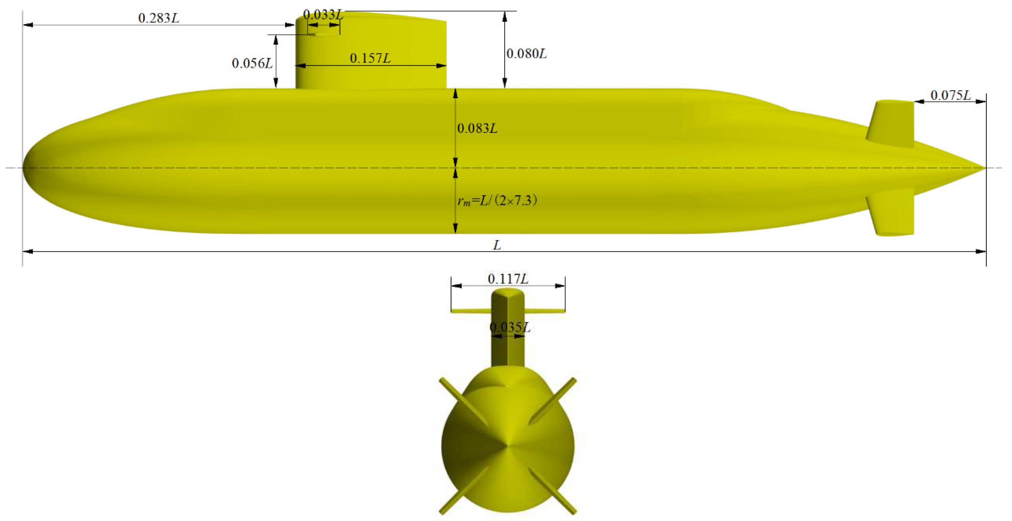
Figure 2.
The schematic diagram of SPIV measurement and wind axis coordinate system (Lee et al., 2019).
Figure 2.
The schematic diagram of SPIV measurement and wind axis coordinate system (Lee et al., 2019).
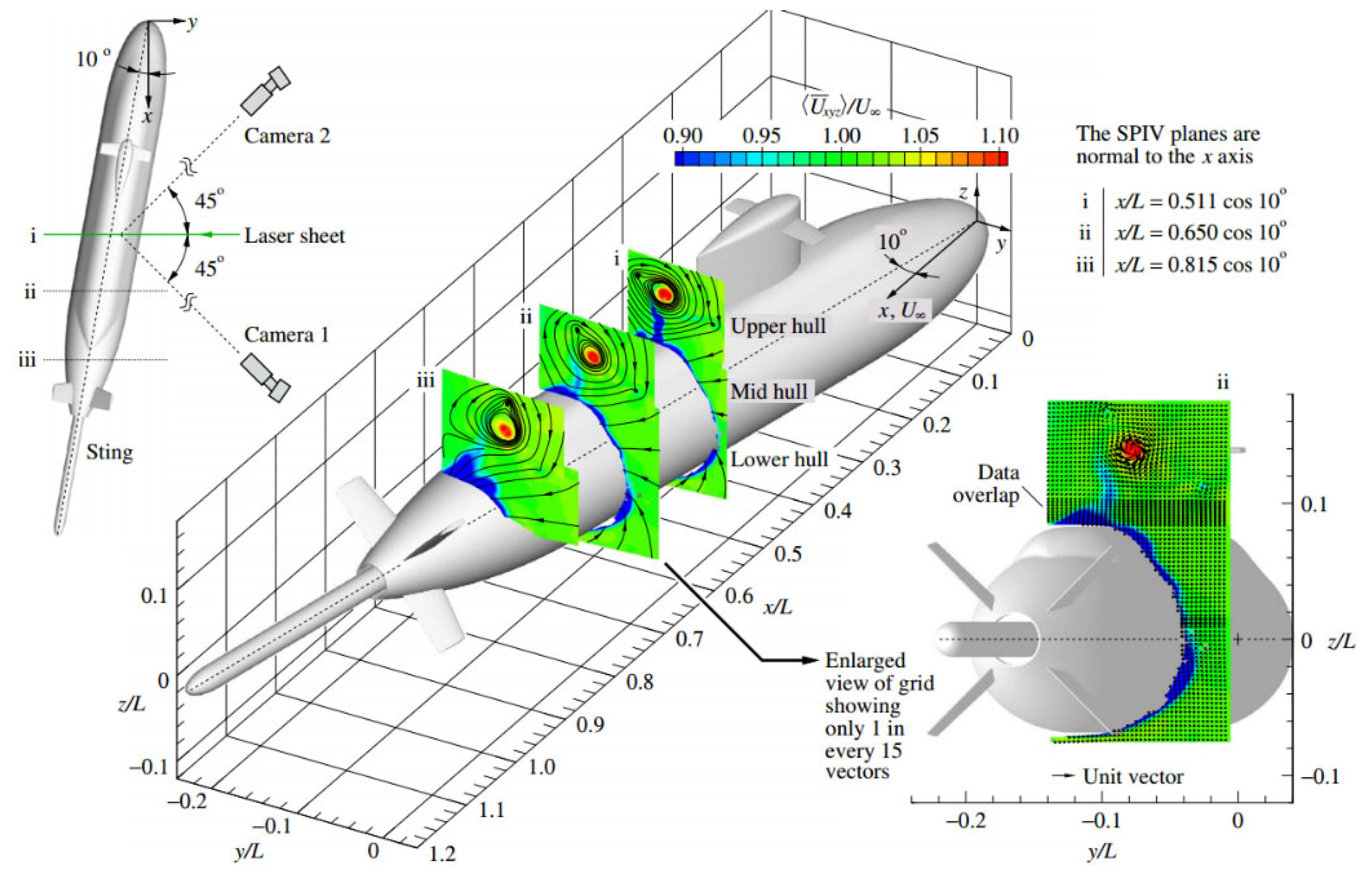
Figure 3.
The computational domain.
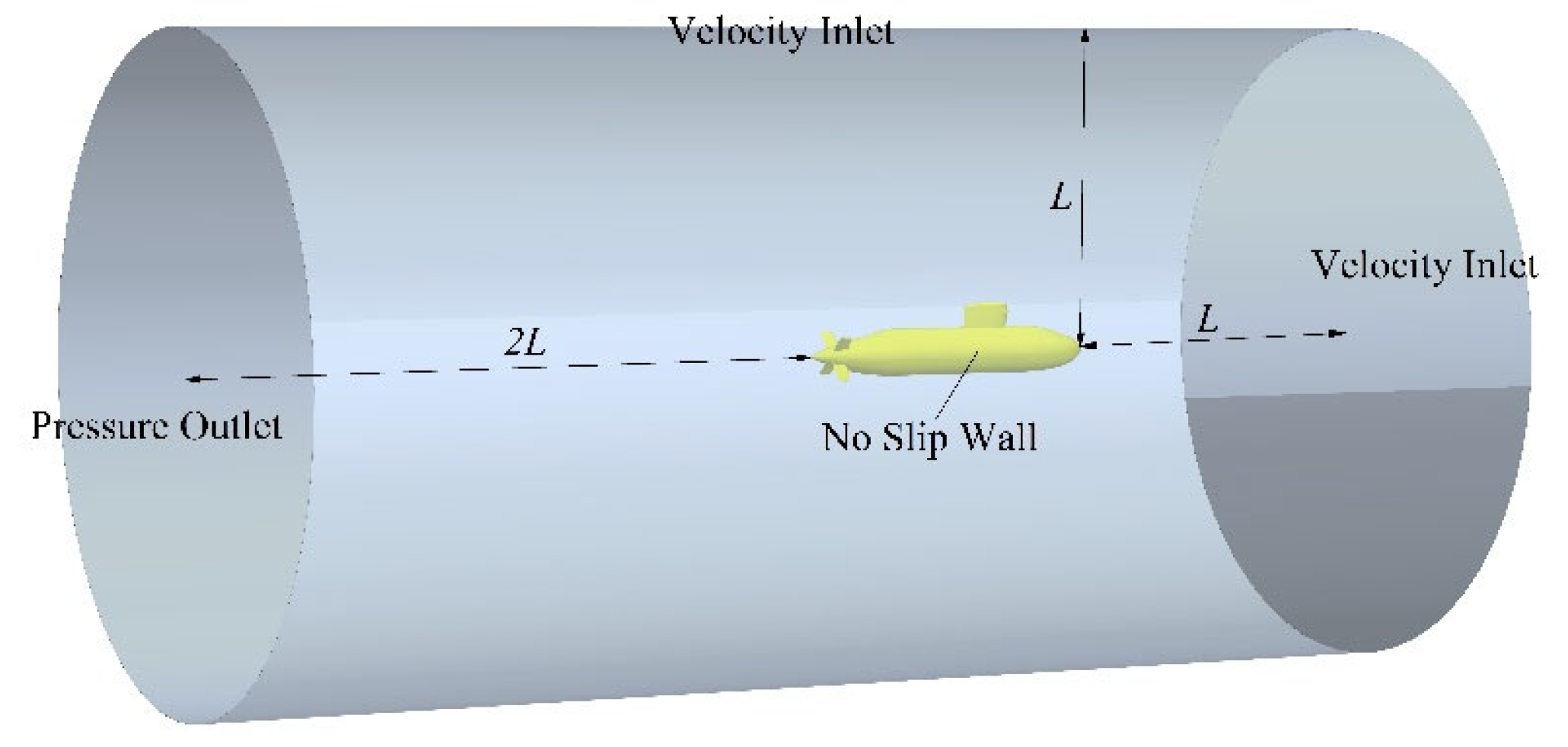
Figure 4.
Grids for computation.
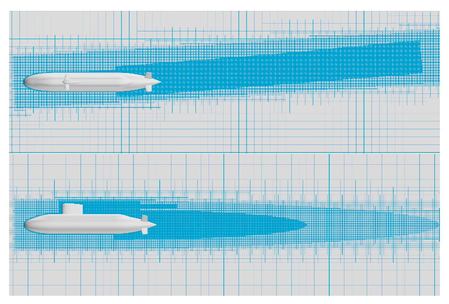

Figure 5.
Comparison of the wake of the cruciform appendage under different sets of grid.
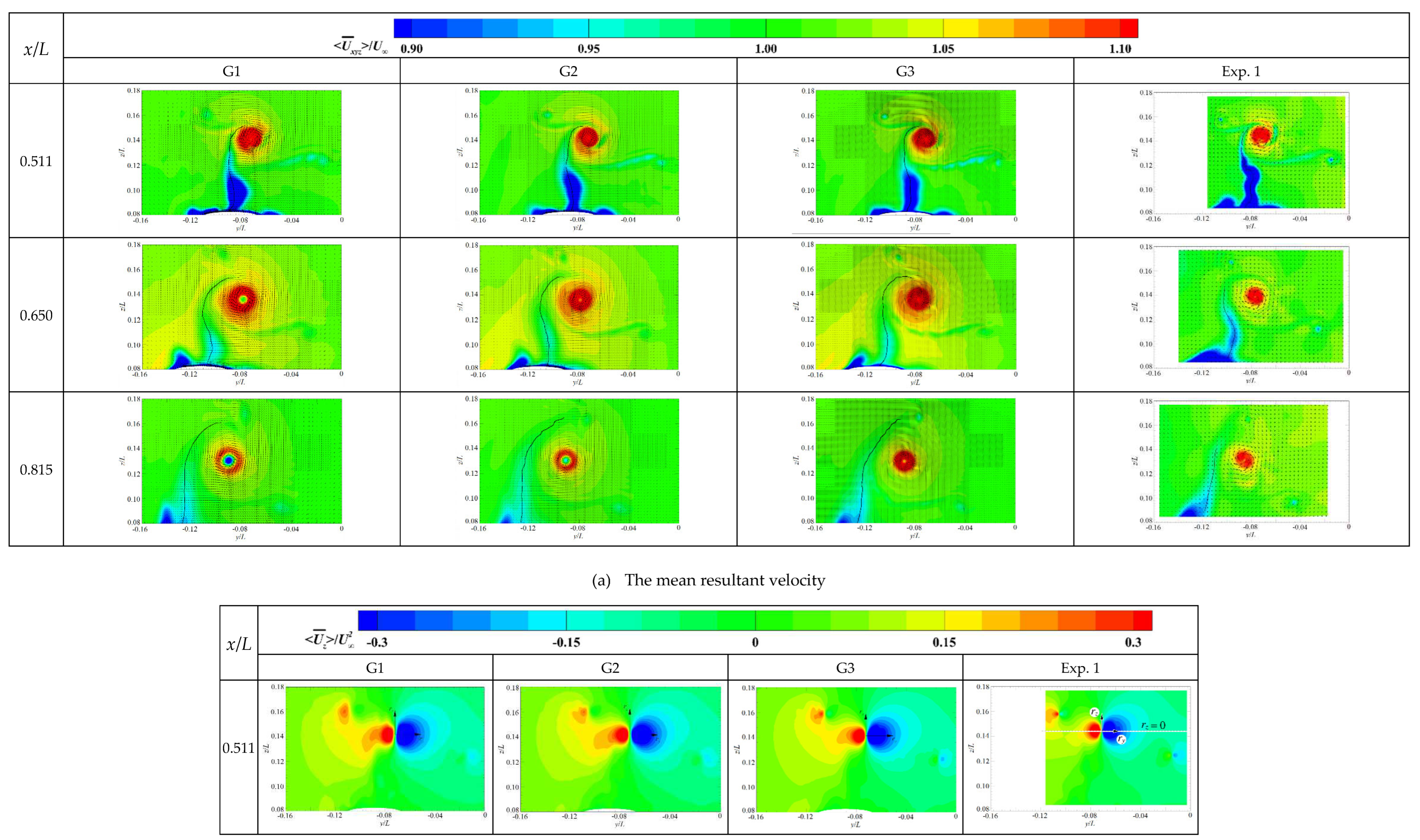
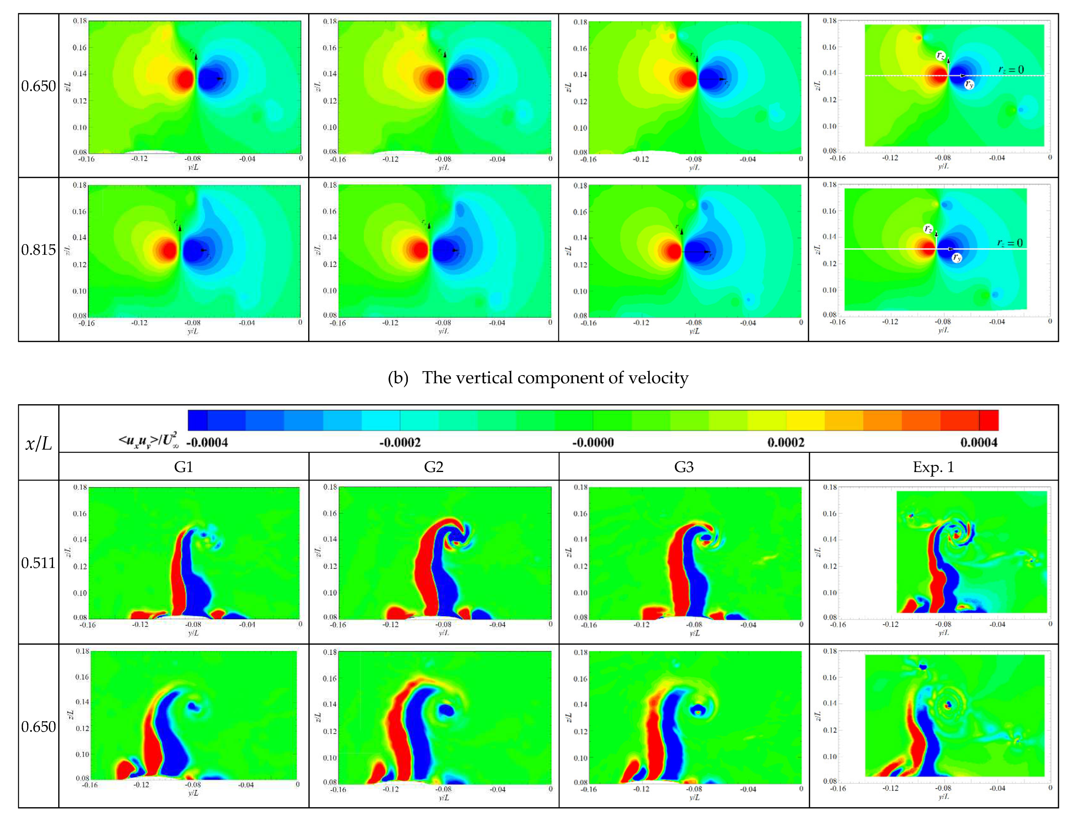
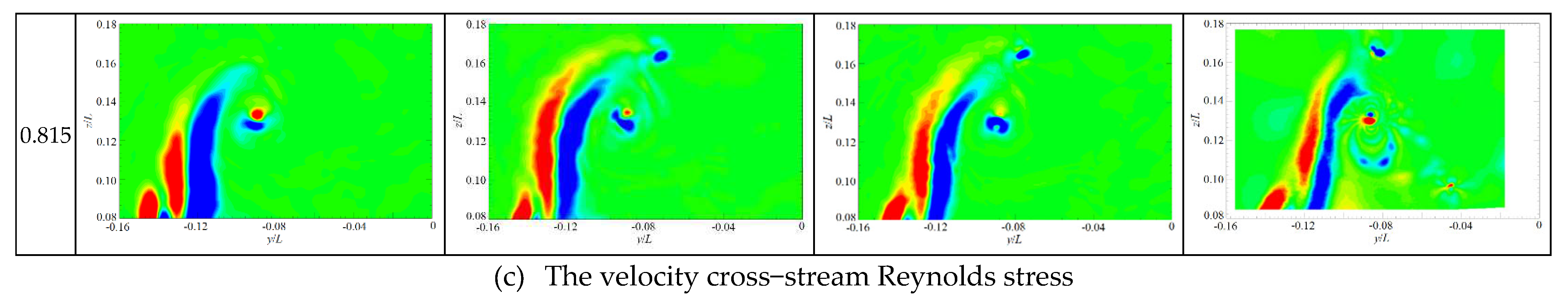
Figure 6.
Comparison of the mean resultant velocity under different sets of grid.
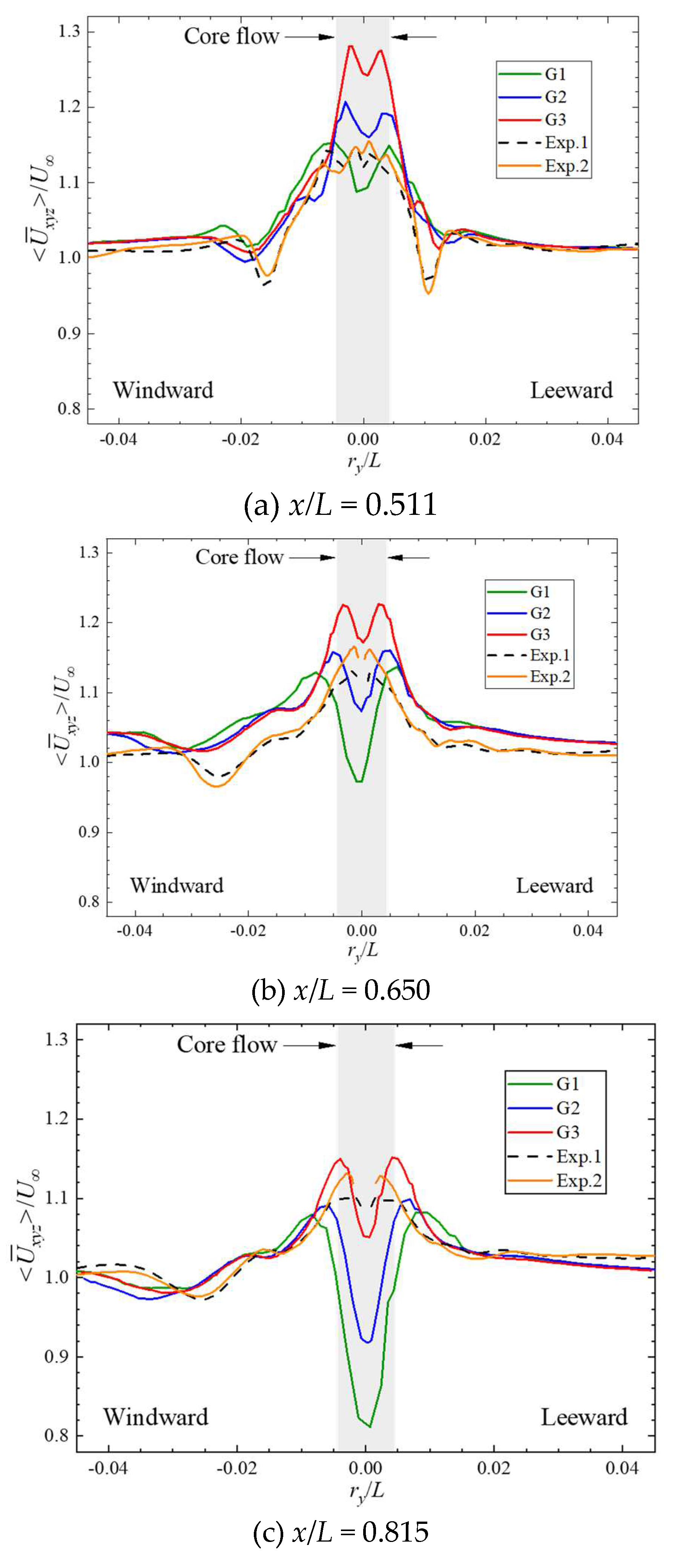
Figure 7.
Comparison of the vertical component of velocity under different sets of grid.
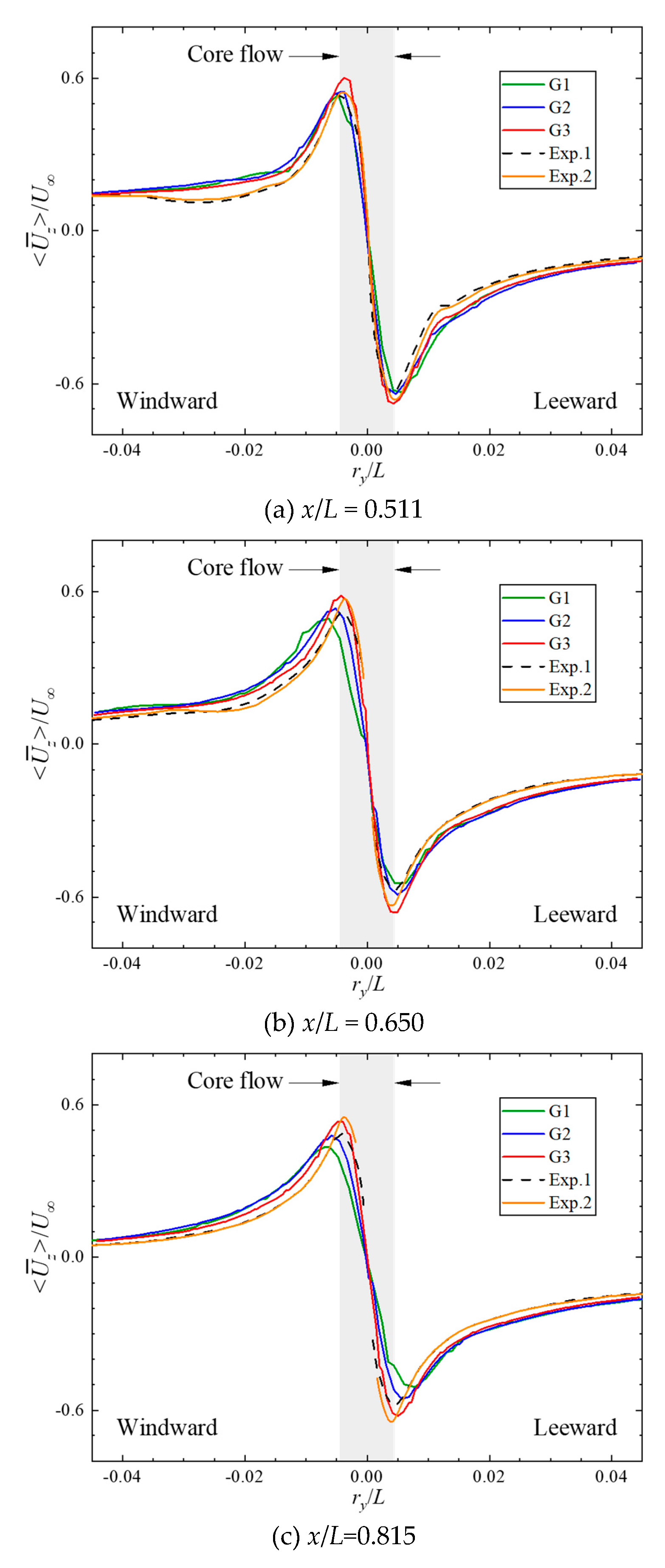
Figure 8.
Comparison of the turbulence kinetic energy under different sets of grid.
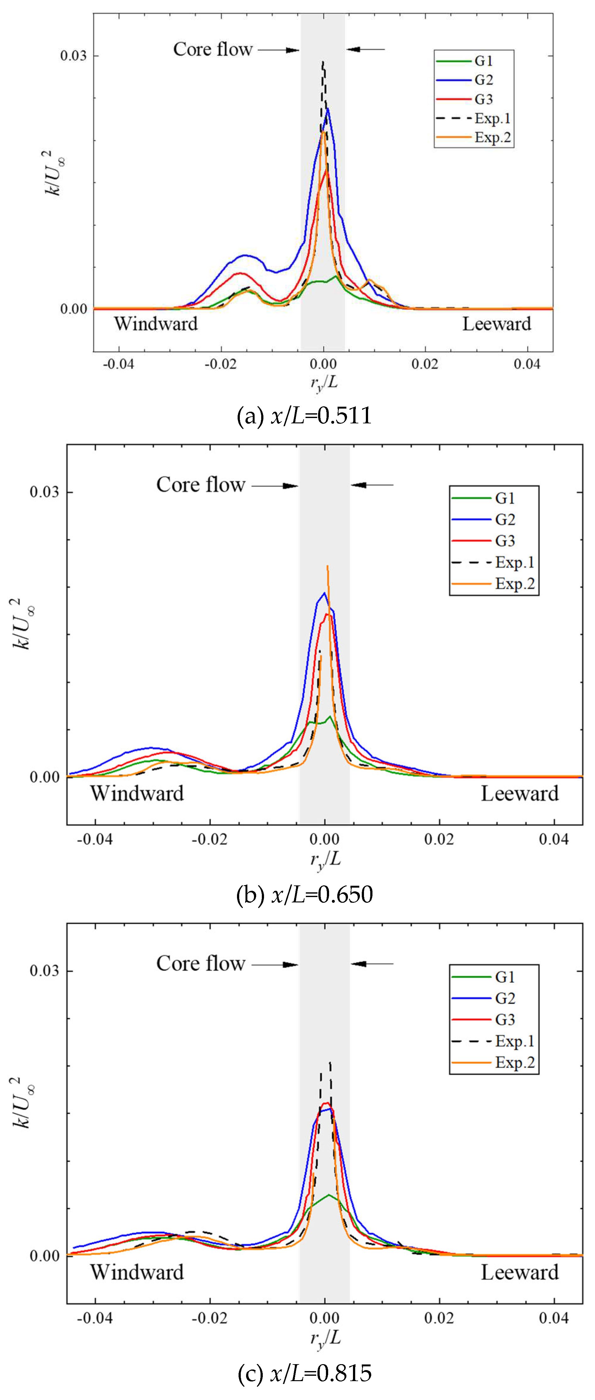
Figure 9.
Comparison of the centerline of the sail wake under different sets of grid.
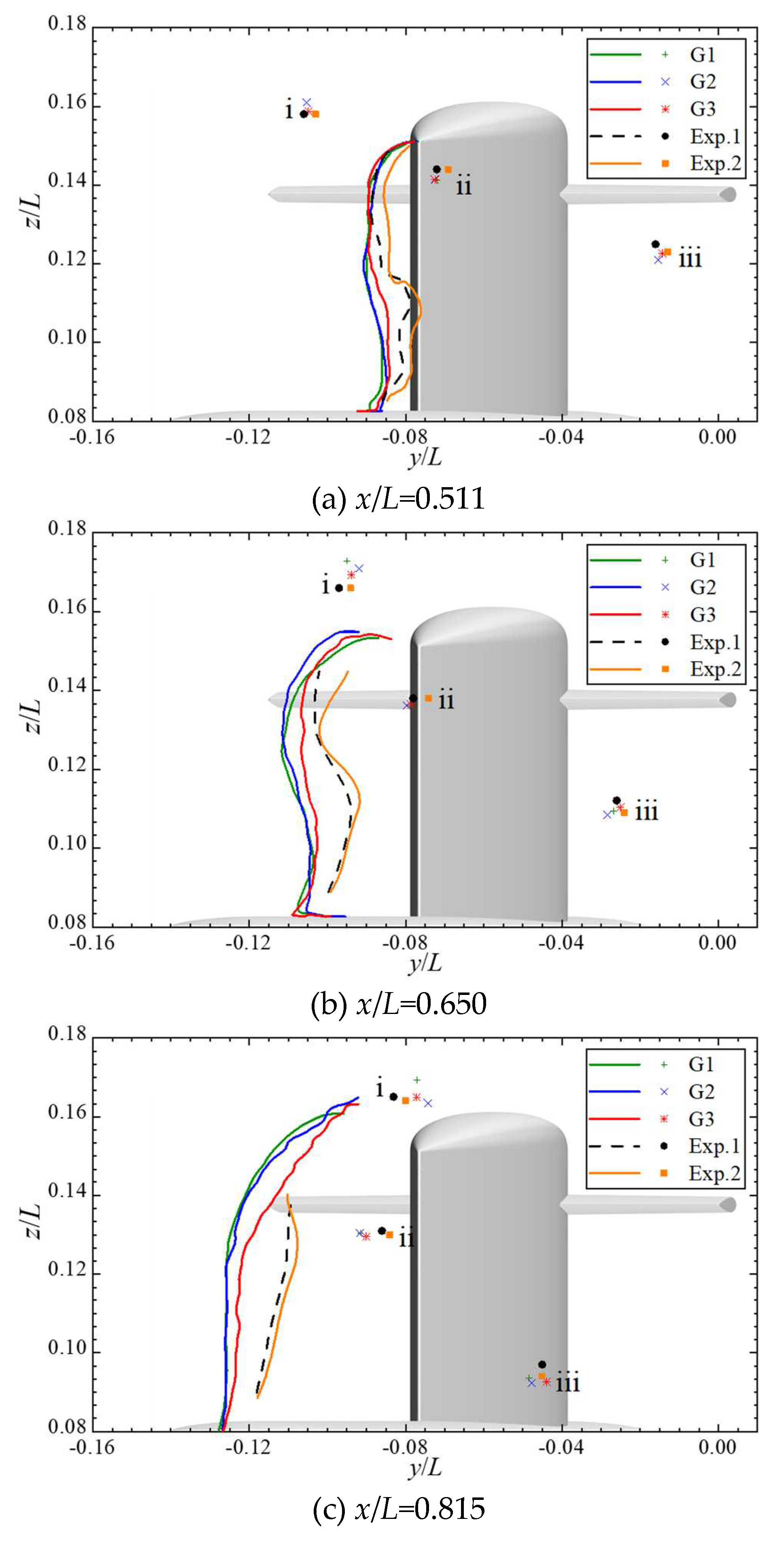
Figure 10.
Development of vortex systems past Joubert BB2 at straight ahead conditions.
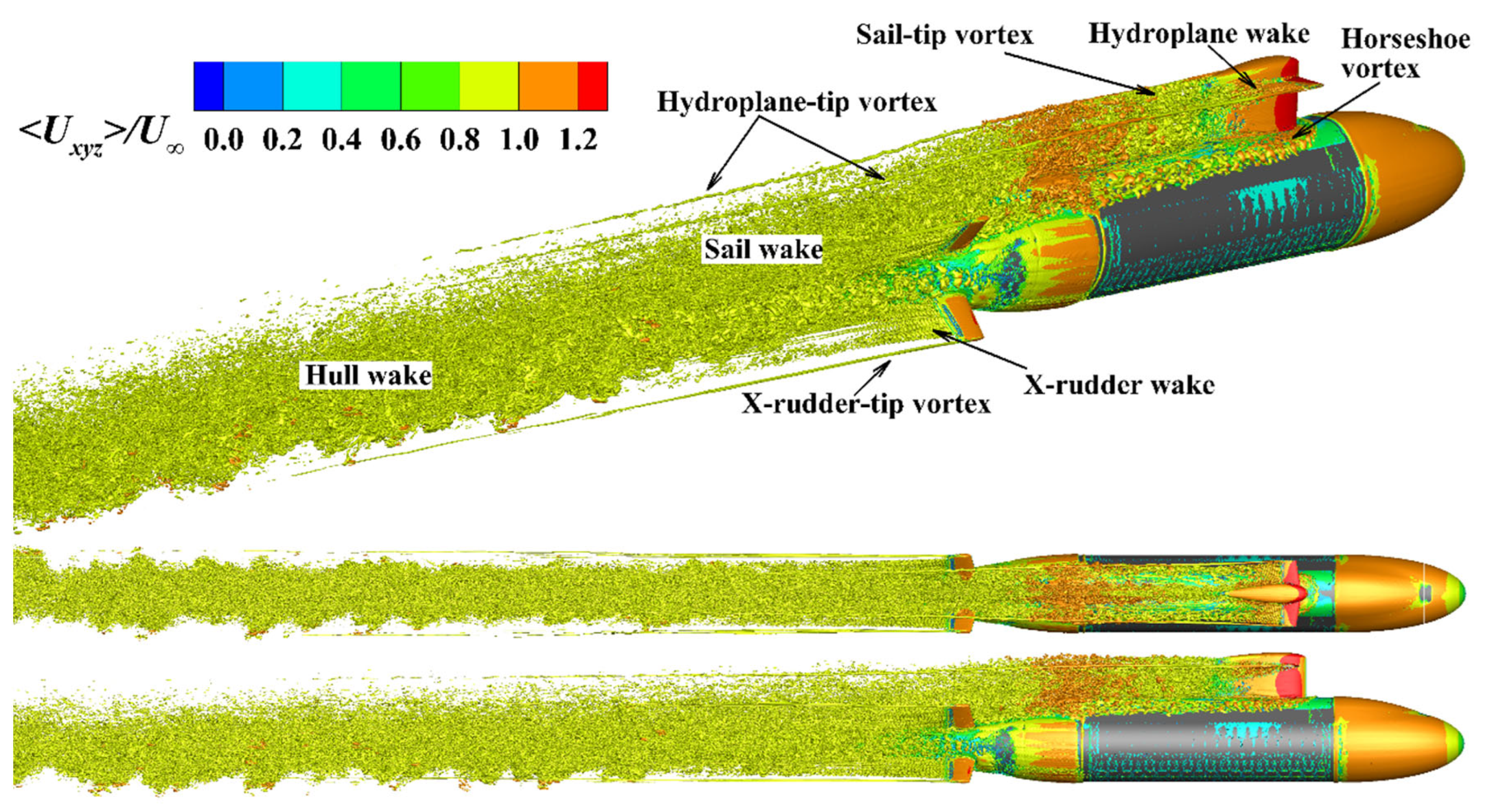
Figure 11.
Development of vortex systems past Joubert BB2 at 10° yaw conditions.
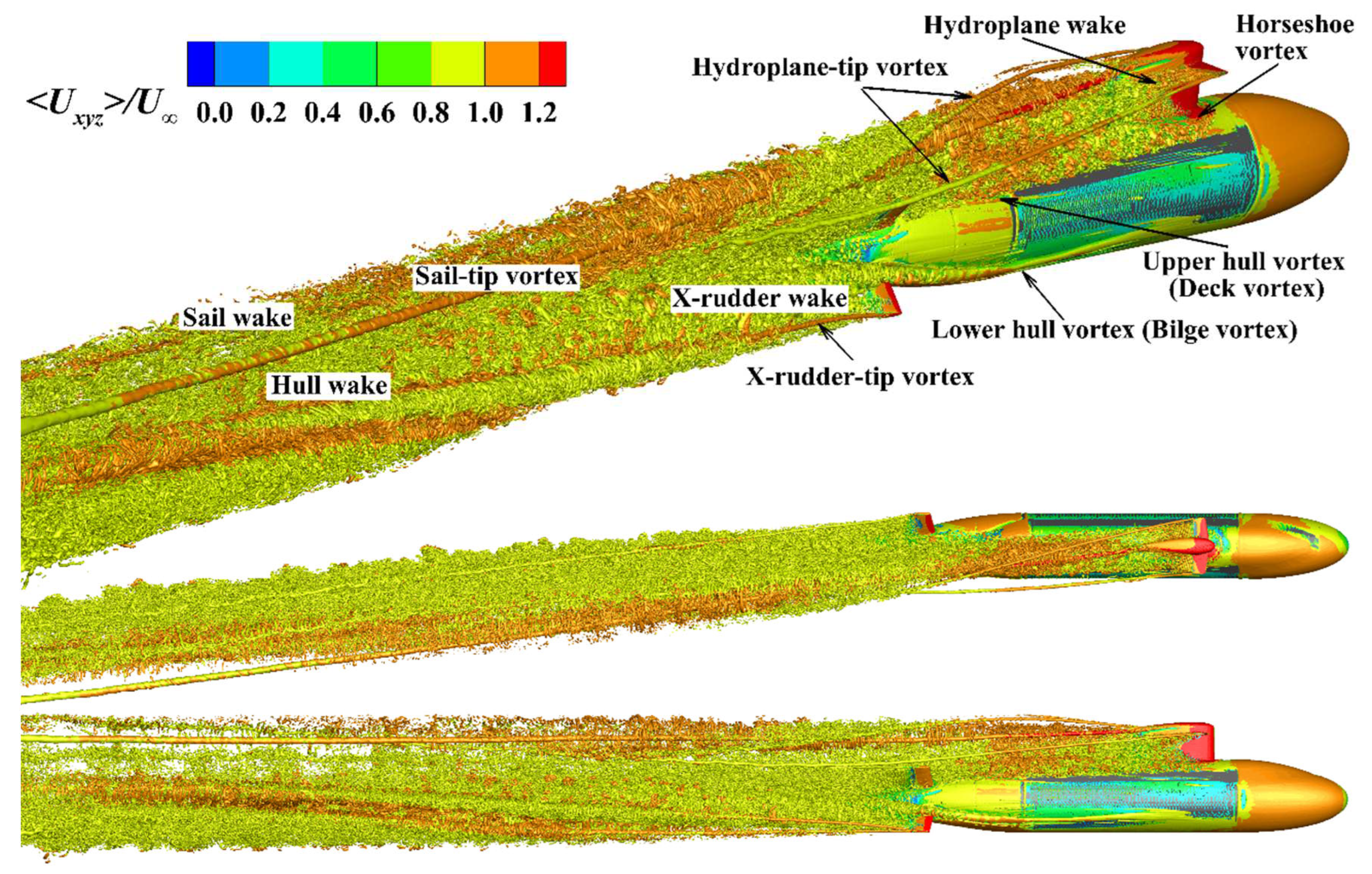
Figure 12.
Trajectories of the cores of tip vortices at 10° yaw conditions.
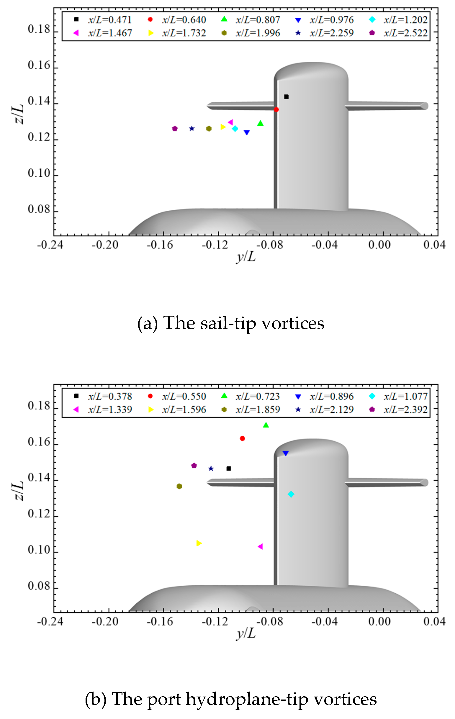
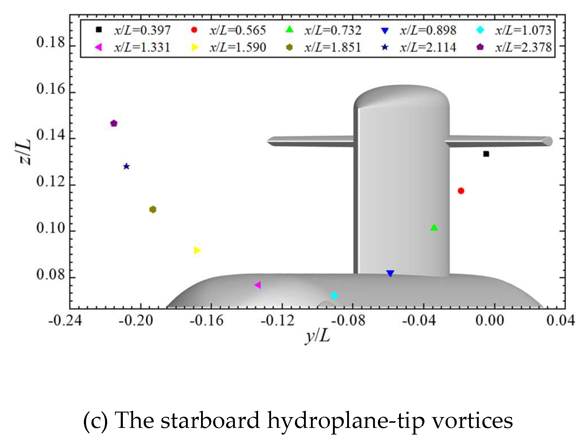
Figure 13.
Evolution of the mean vorticity magnitude.
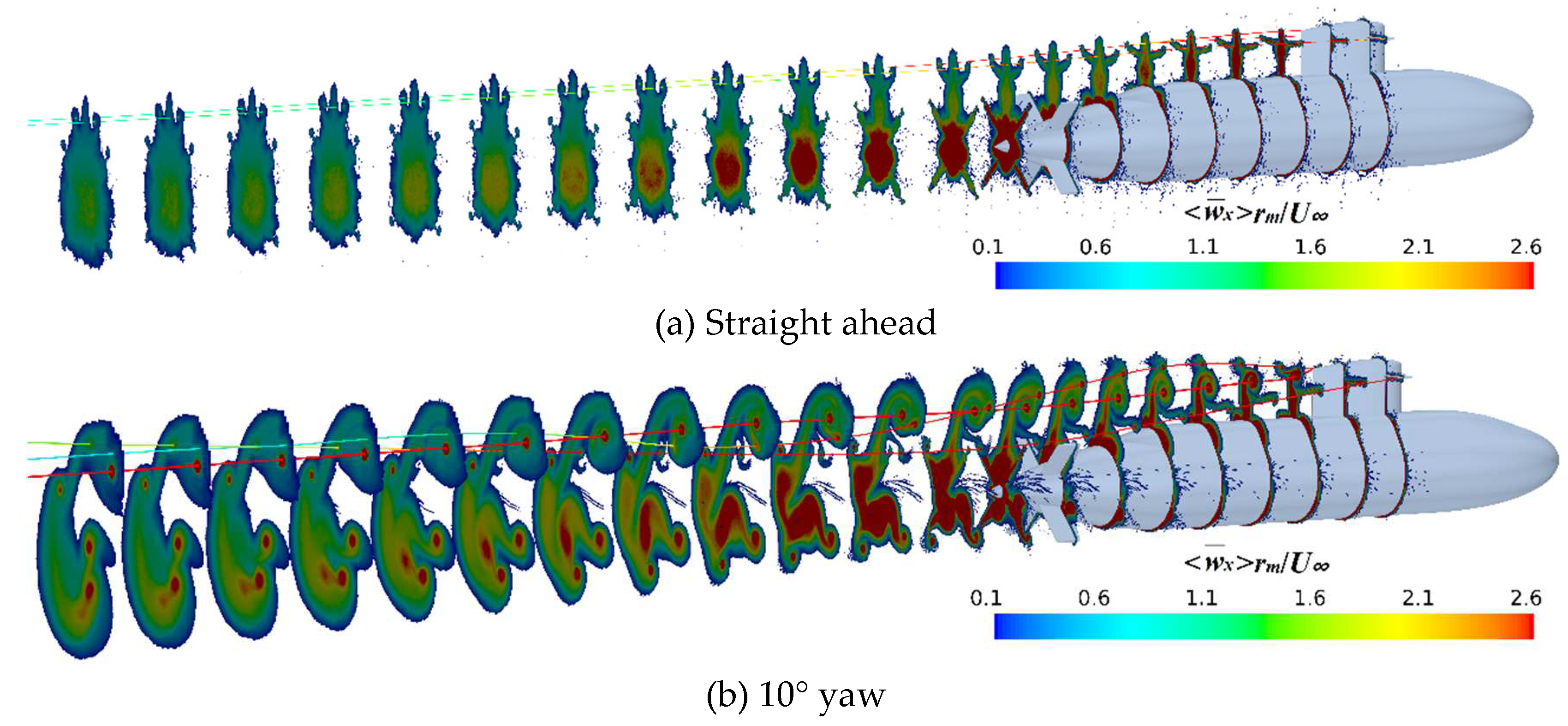
Figure 14.
Evolution of the turbulence kinetic energy.
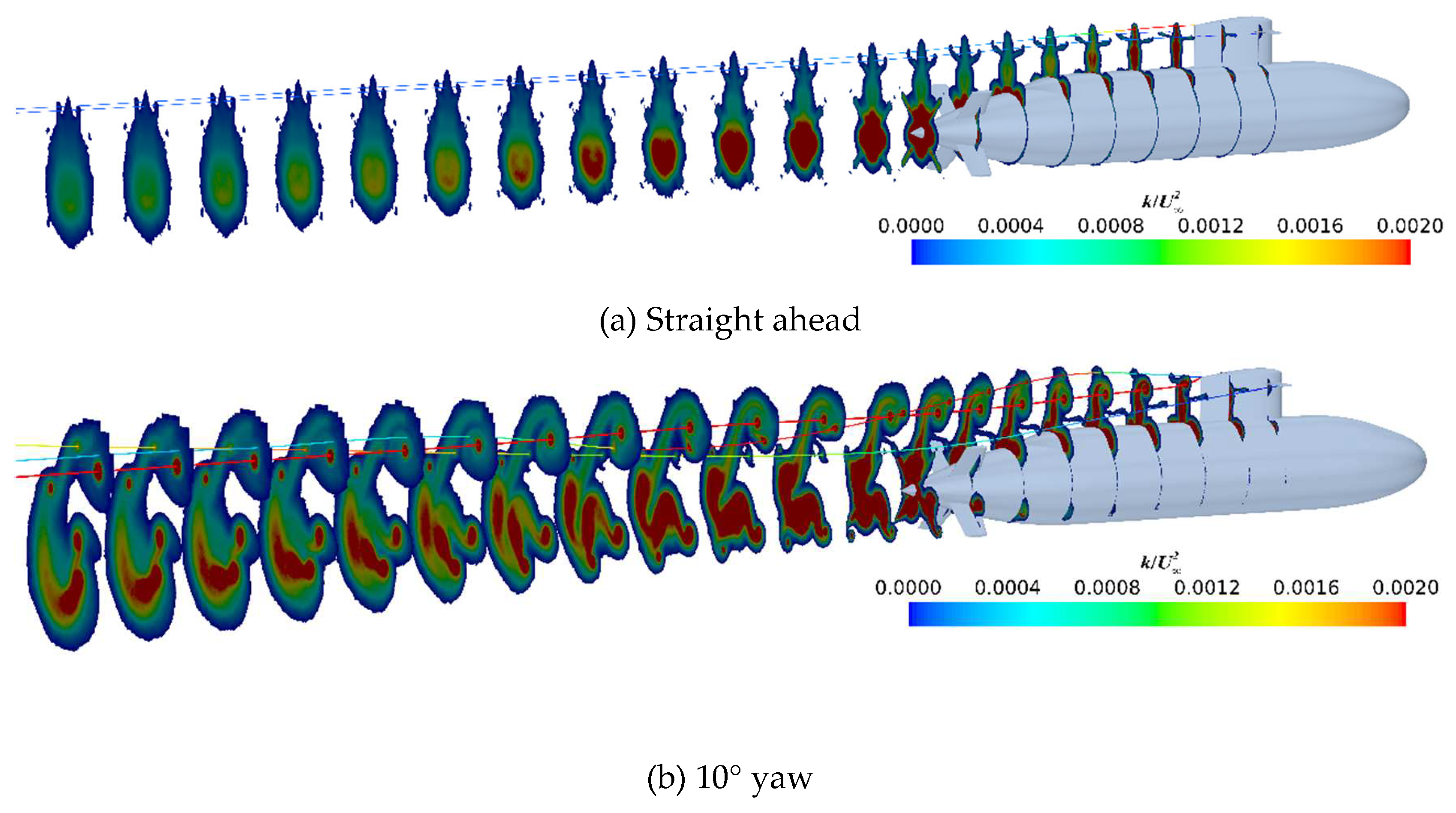
Figure 15.
Comparison of the mean resultant velocity at straight ahead and 10° yaw conditions.
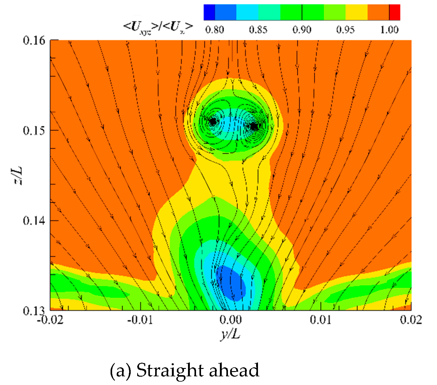
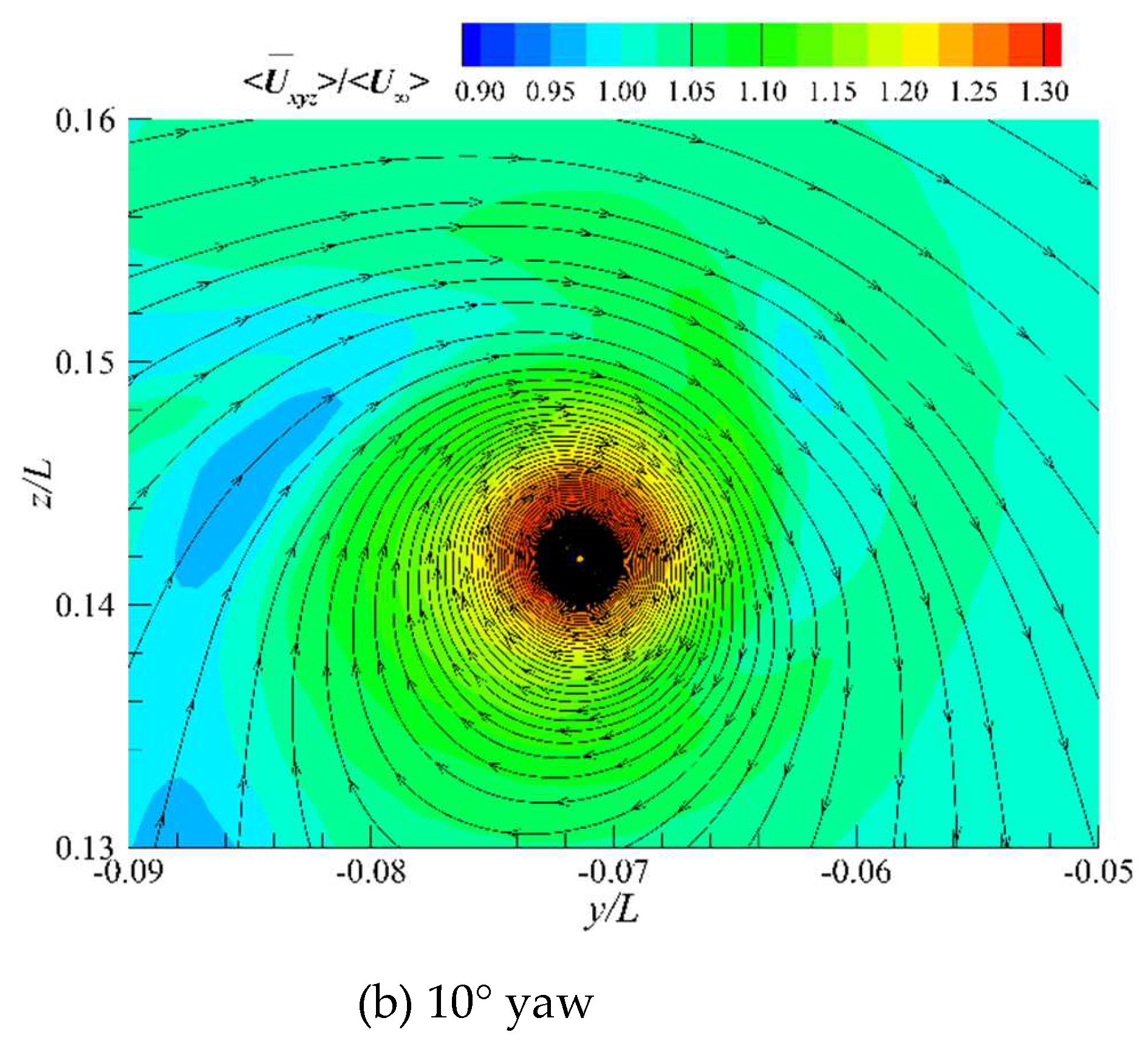
Figure 16.
Comparison of the mean vorticity magnitude at straight ahead and 10° yaw conditions.
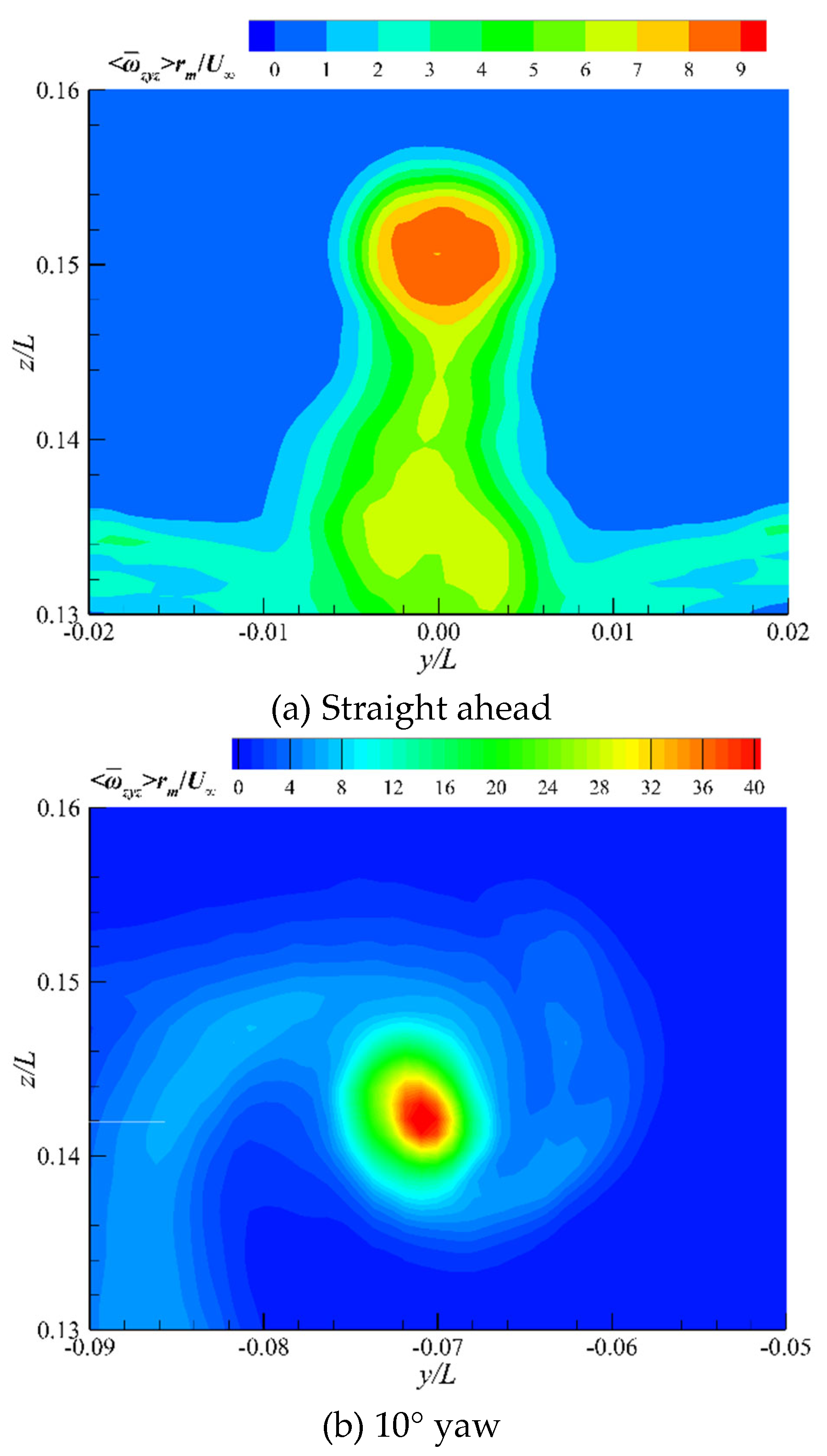
Figure 17.
Comparison of the turbulence kinetic energy at straight ahead and 10° yaw conditions.
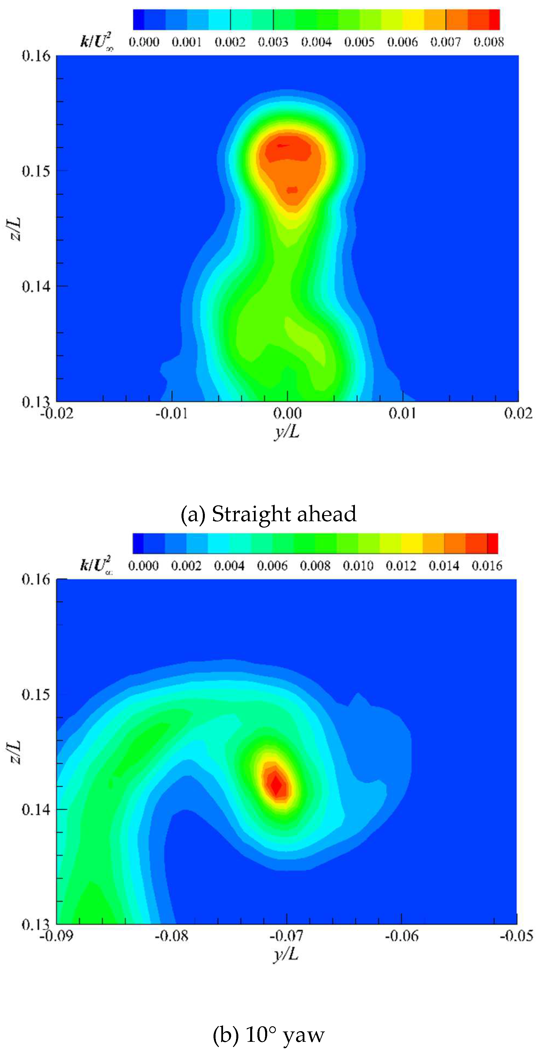
Figure 18.
Comparison of the mean velocity under different streamwise locations.
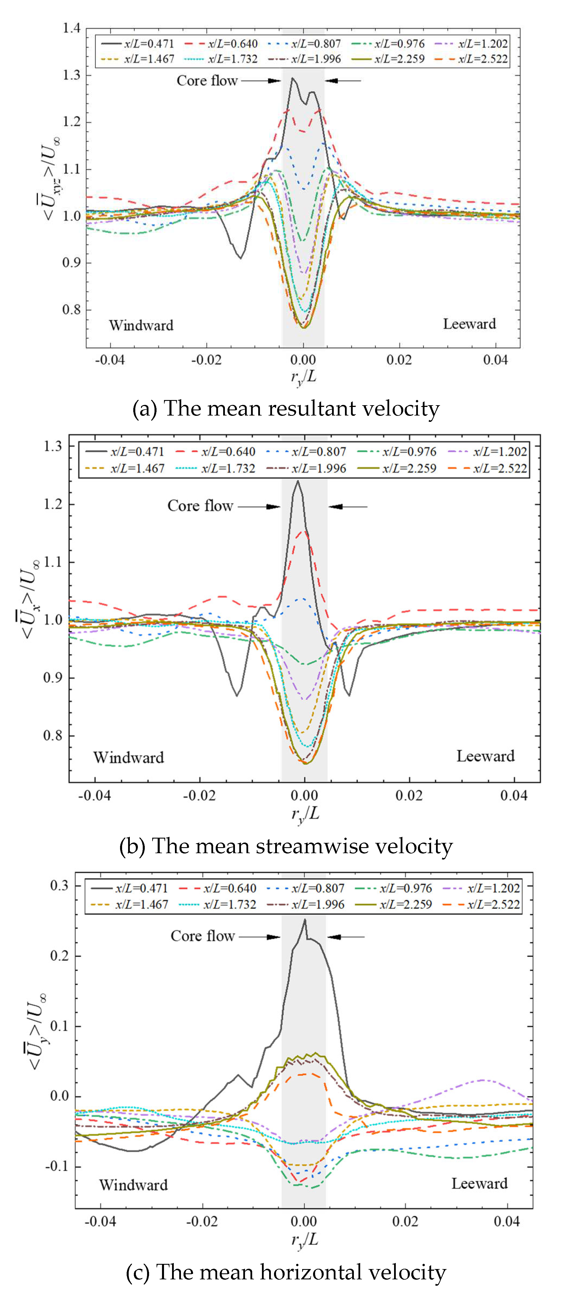
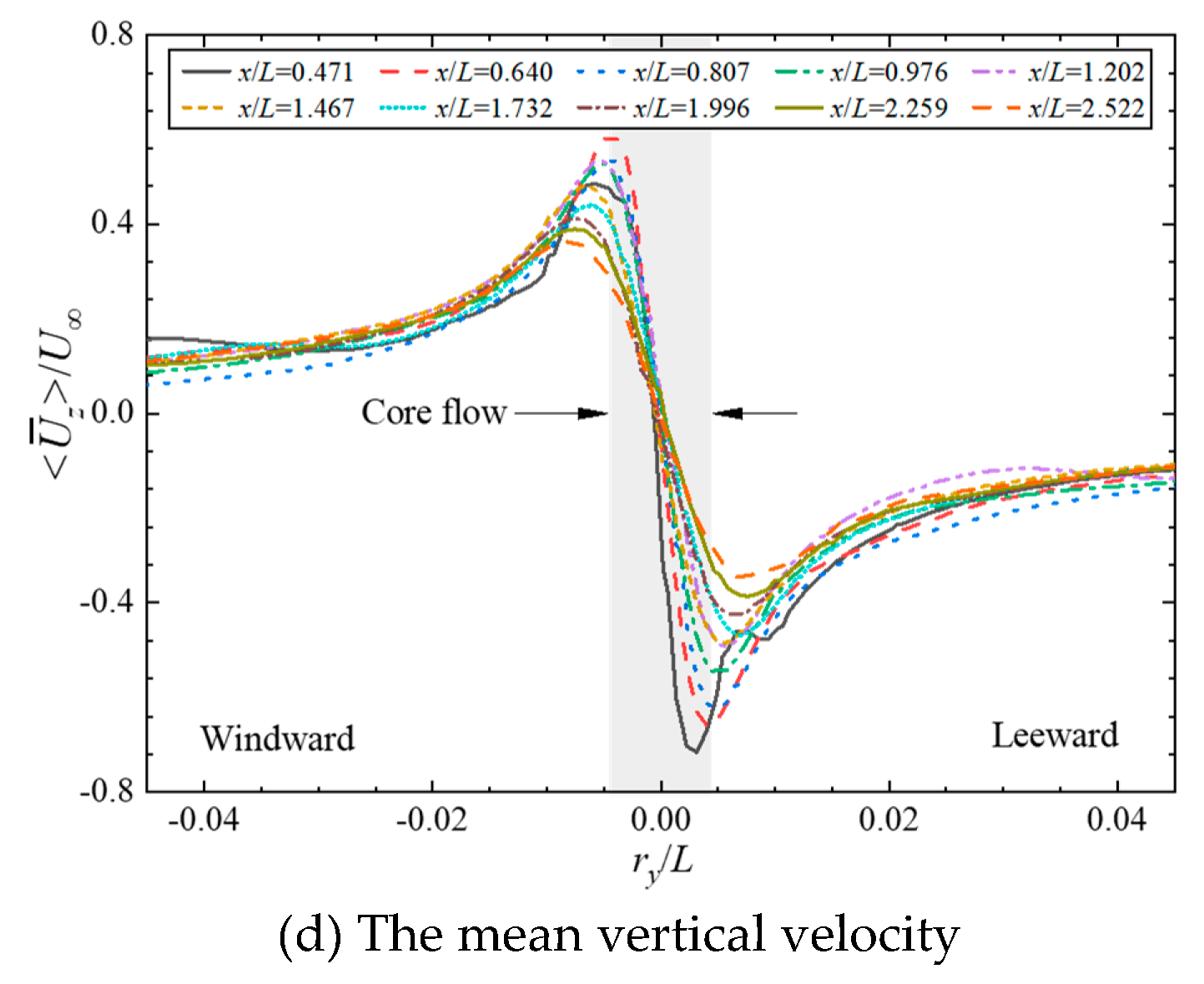
Figure 19.
Comparison of the mean vorticity under different streamwise locations.
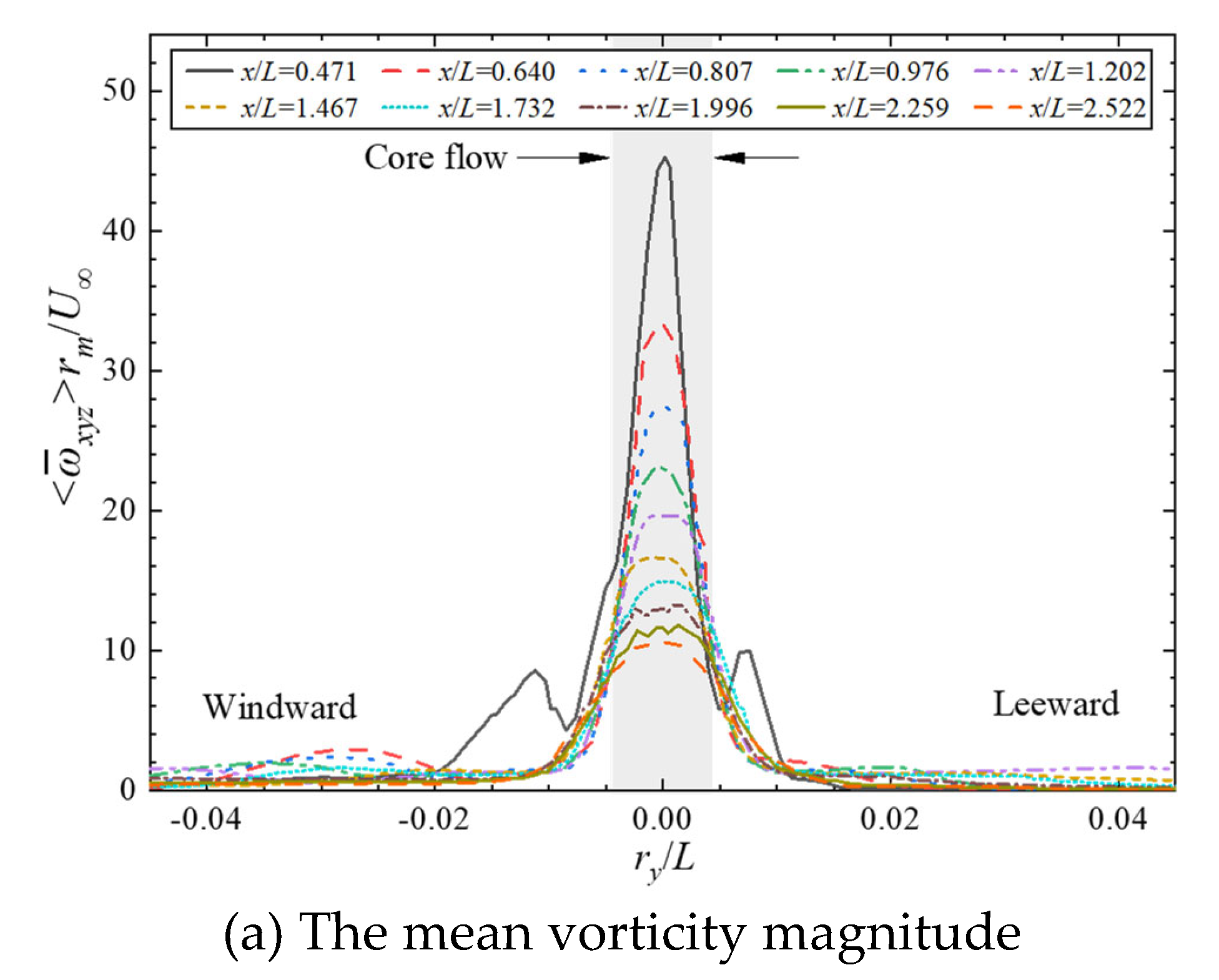
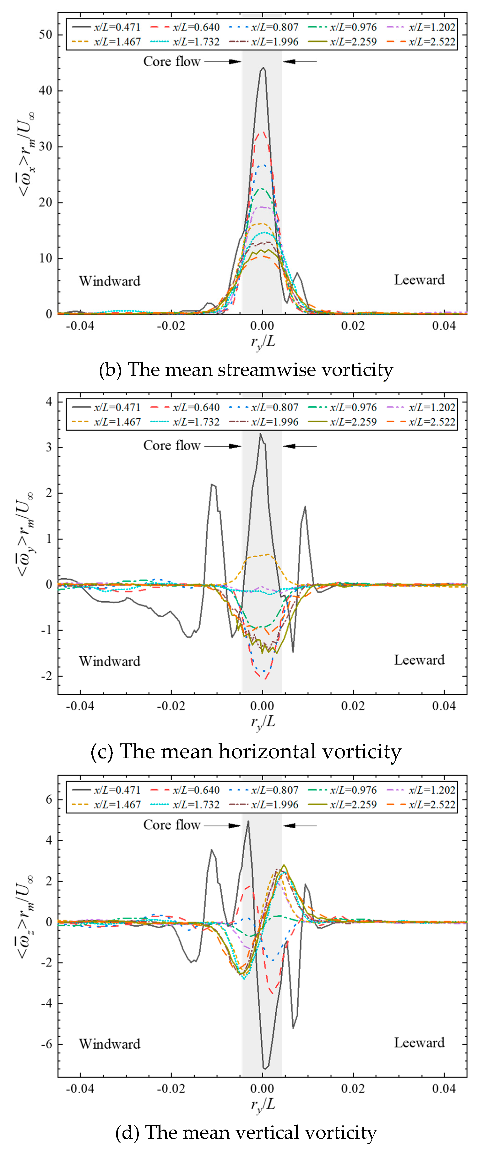
Figure 20.
Comparison of the turbulence kinetic energy under different streamwise locations.
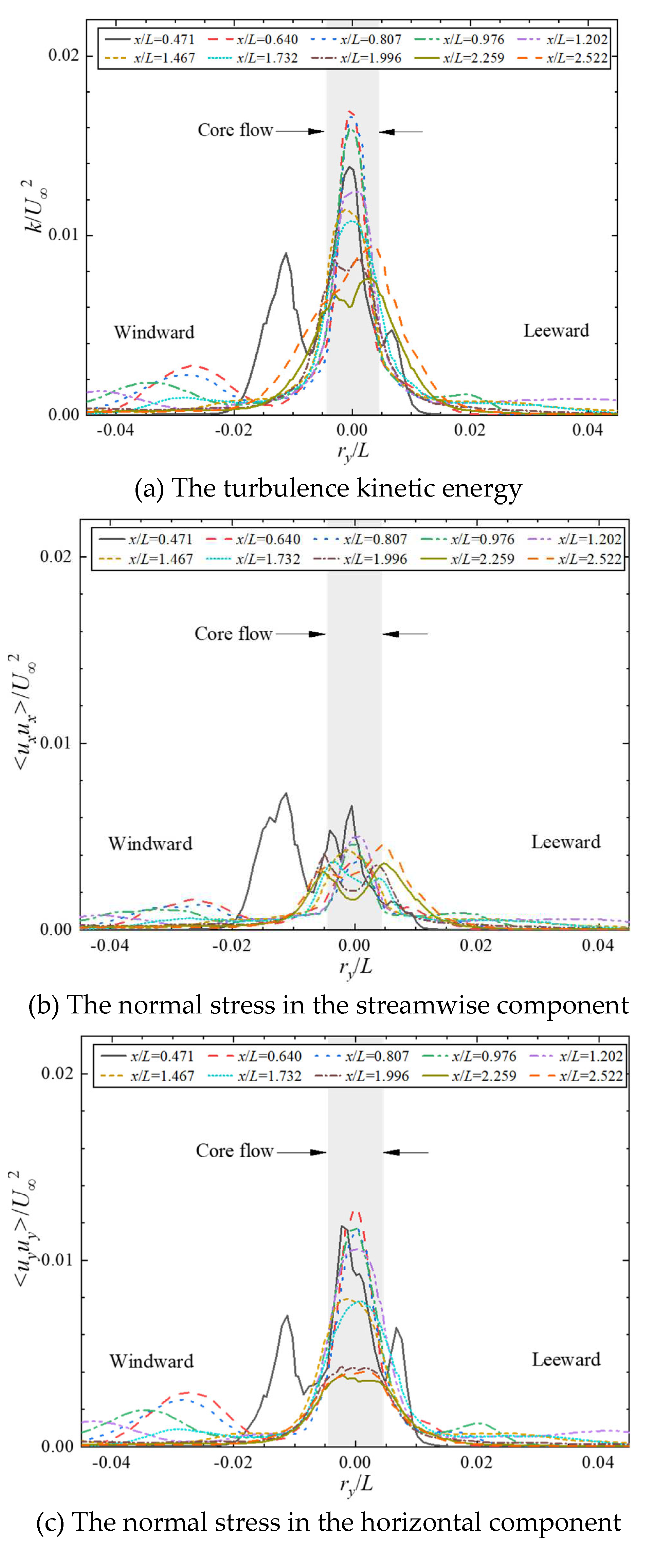
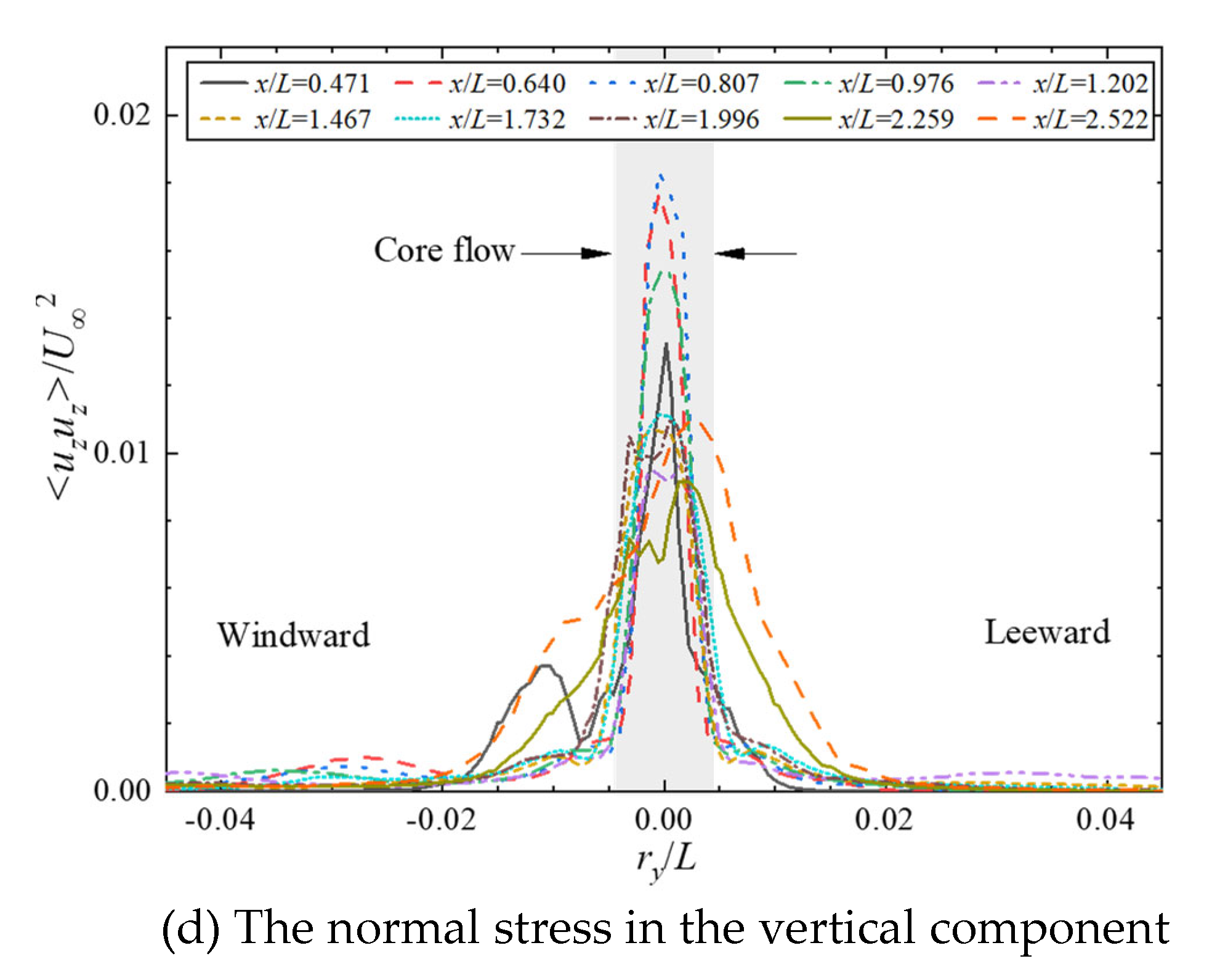

Table 1.
Summary of the centers of the vortices on the upper hull.
| Measurement Plane | Grid Scheme | Sail tip | Hydroplanes | ||||
| Windward | Leeward | ||||||
| y/L | z/L | y/L | z/L | y/L | z/L | ||
| G1 | −0.072 | 0.141 | −0.108 | 0.161 | −0.013 | 0.123 | |
| x/L=0.511 | G2 | −0.073 | 0.141 | −0.105 | 0.161 | −0.015 | 0.121 |
| G3 | −0.072 | 0.141 | −0.105 | 0.159 | −0.014 | 0.123 | |
| G1 | −0.079 | 0.136 | −0.095 | 0.173 | −0.027 | 0.109 | |
| x/L=0.650 | G2 | −0.080 | 0.136 | −0.092 | 0.171 | −0.028 | 0.109 |
| G3 | −0.079 | 0.136 | −0.094 | 0.169 | −0.025 | 0.110 | |
| G1 | −0.092 | 0.130 | −0.077 | 0.169 | −0.048 | 0.094 | |
| x/L=0.815 | G2 | −0.092 | 0.130 | −0.074 | 0.163 | −0.048 | 0.092 |
| G3 | −0.090 | 0.130 | −0.077 | 0.165 | −0.044 | 0.093 | |
Table 2.
Summary of the relative errors to Exp. 2 of the centers of the vortices.
| Measurement Plane | Grid Scheme | Sail tip | Hydroplanes | ||||
| Windward | Leeward | ||||||
| y/L(%) | z/L(%) | y/L(%) | z/L(%) | y/L(%) | z/L(%) | ||
| G1 | 4.3 | −1.9 | 5.3 | 1.6 | 2.7 | 0.3 | |
| x/L=0.511 | G2 | 5.3 | −1.8 | 2.2 | 1.9 | 18.2 | −1.6 |
| G3 | 5.0 | −1.9 | 1.8 | 0.5 | 10.7 | −0.3 | |
| G1 | 6.5 | −1.3 | 1.0 | 4.2 | 12.0 | 0.4 | |
| x/L=0.650 | G2 | 7.7 | −1.4 | −2.3 | 3.0 | 18.6 | −0.4 |
| G3 | 6.1 | −1.1 | −0.1 | 2.0 | 4.8 | 1.2 | |
| G1 | 9.0 | 0.4 | −3.7 | 3.3 | 7.5 | −0.5 | |
| x/L=0.815 | G2 | 9.2 | 0.3 | −7.0 | −0.4 | 6.2 | −1.8 |
| G3 | 7.2 | −0.3 | −3.5 | 0.6 | −2.5 | −1.5 | |
Disclaimer/Publisher’s Note: The statements, opinions and data contained in all publications are solely those of the individual author(s) and contributor(s) and not of MDPI and/or the editor(s). MDPI and/or the editor(s) disclaim responsibility for any injury to people or property resulting from any ideas, methods, instructions or products referred to in the content. |
© 2023 by the authors. Licensee MDPI, Basel, Switzerland. This article is an open access article distributed under the terms and conditions of the Creative Commons Attribution (CC BY) license (http://creativecommons.org/licenses/by/4.0/).
Copyright: This open access article is published under a Creative Commons CC BY 4.0 license, which permit the free download, distribution, and reuse, provided that the author and preprint are cited in any reuse.


