
Submitted:
07 November 2023
Posted:
08 November 2023
You are already at the latest version
Abstract
Solar flares are broadly classified as impulsive or gradual. Ions accelerated in a gradual flare are thought to be accelerated through a shock acceleration mechanism, but the particle acceleration process in an impulsive flare is still largely unexplored. To understand the acceleration process, it is necessary to measure the high-energy gamma-rays and neutrons produced by the impulsive flare. Under such circumstances, on November 7, 2004, a huge X2.0 flare occurred on the solar surface, where ions were accelerated to energies greater than 10 GeV. The accelerated primary protons collided with the solar atmosphere and produced line gamma-rays and neutrons. These particles were received as neutrons and line gamma-rays, respectively. Neutrons of a few GeV, on the other hand, decay to produce secondary protons while traveling 0.06 au in the solar-terrestrial space. These secondary protons arrived at the magnetopause. Although the flux of secondary protons is very low, the effect of collecting secondary protons arriving in a wide region of the magnetosphere (the Funnel or Horn effect) has resulted in significant signals being received by the solar neutron telescope at Mt. Sierra Negra (4,600 m). This information suggests that ions on the solar surface are accelerated to over 10 GeV with an impulsive flare.
Keywords:
solar flare
; impulsive flare
; gradual flare
; solar comic-rays
; solar energetic particles
; particle acceleration
; solar neutrons
1. Introduction
In association with solar flares, ions are accelerated to high energies and arrive on the Earth. These high-energy ions are called solar cosmic rays, districting from galactic cosmic rays. However, it still needs to be clarified what energies the galactic cosmic rays are accelerated, where they are accelerated, and their acceleration mechanism. The acceleration mechanism for the solar cosmic rays produced by solar flares remains as a puzzle to be understood. Solar flares are used to be classified into two types: the impulsive flare and the gradual flare. For more details on this classification, refer to the paper written by Don Reames in this special issue [1,2].
Solar cosmic rays produced by the gradual flares have been attributed to the gradual acceleration of ions by their reciprocal motion across the shock inside the Coronal Mass Ejection (CME) that is observed in association with the event. However, the hypothesis of acceleration by shock waves fails to explain the observed short-term acceleration of energetic ions in impulsive flares. To illustrate this phenomenon, Holman, Litvinenko, Somov proposed the electric field acceleration model in the 1995 [3,4,5], which produces high-energy ions in a shorter duration. However, there is still no clear observational evidence supporting this model.
Fisk has proposed the wave-riding theory in order to explain the low-energy abundance of 3He and Fe ions [6,7]. However, this model is classified into a 2nd-order Fermi acceleration mechanism [8], which means it can’t quickly accelerate particles to high energies. Therefore, it is crucial to capture as many solar cosmic rays associated with the impulsive flare as possible. To do this, we must detect high-energy solar cosmic rays and simultaneously must observe the X-ray, gamma-ray and ultraviolet images on the solar surface. This is what we refer to as the solar version of the multi-messenger astronomy.
Observation of high-energy solar particle beams requires a great deal of ingenuity due to the presence of a magnetic field between the Sun and Earth, which is created by the solar dynamo activity and has a strength of approximately 5 nT near the Earth. The magnetic field causes the effect of the trajectory of charged particles from the Sun to the Earth. They are transported in the Parker field and transferred to the Earth not straightforwardly. Therefore, this leads to an orbit dependence for charged particles on the arrival time of the particles, longer than the light that travels straightforwardly. As a result, these data cannot be compared with the optical phenomena such as gamma-rays, ultraviolet rays and X-rays on the solar surface. To avoid the time lag problem, we used to compare the data with optical phenomena on the solar surface in case high-energy neutral particles such as gamma-rays and neutrons are detected. Therefore, the detection of these neutral particle rays is expected to clarify the acceleration processes of protons and electrons in the impulsive flare.
Neutrons have mass, which means they take longer time to travel through solar-terrestrial space than light. However, this issue can be resolved by measuring the neutron’s energy. Figure 1 displays the relationship between the energy of a neutron and the flight time traveling through 1 astronomical unit (1 au) of space. For example, a neutron with an energy of 100 MeV will lag behind light by approximately 660 seconds, whereas a neutron with an energy of 400 MeV will have a delay time of 200 seconds. At an energy level of 1000 MeV, the time difference between the neutron and light is only one minute. When the detector threshold is set at 30 MeV, which will be discussed in the next chapter, the delay time is 1,460 seconds (approximately 24 minutes), and at 40 MeV, it turns out as 1,280 seconds (approximately 21 minutes). If solar neutrons are produced on the solar surface in a -functional time distribution, they should be detected by our instruments within about 20 minutes.
However, during their journey over 1 au, neutrons decay into protons, electrons, and antineutrinos. Therefore, we must take this effect into account when determining the flux. For example, at an energy level of 70 MeV, 70 % of neutrons decay during their 1 au flight, and the probability of survival is around 30 %. On the other hand, at an energy level of 1 GeV, 92.5 % of neutrons do not decay and reach the Earth.
Unlike high-energy gamma-rays, neutrons are only produced by collisions of ions with solar atmosphere. Therefore, information on pure ions can be obtained from them, but the above correction is associated. Gamma-rays are also generated by electron bremsstrahlung and also by the decay of neutral mesons () produced by the nuclear collisions of neutrons with the solar atmosphere. Hence, it will lead to an unclear problem of whether gamma-rays are produced by ions or electrons.
Figure 2 provides an example of the first detection of solar neutrons [9]. The Gamma-Ray Spectrometer onboard the Solar Maximum Mission satellite detected the signal, and the neutron monitor located at Jungfraujoch high altitude confirmed the increase of neutrons after one minute later. The peak at 11:43:30 UT was caused by a gamma-ray flash, while the signal arrived one minute later and is estimated to be 1 GeV with the energy of neutrons.
In Figure 3, the event of May 24, 1990, is presented. The Soviet satellite GRANAT received a strong gamma-ray flash due to this event, which had a gamma-ray peak of 10.6-109.5 MeV at 20:48:10 UT. At the same time, a neutron monitor located in North America recorded an arrival of massive neutrons with a rise time at 20:49 UT, with a time difference of approximately one minute [10,11]. Moreover, an accelerated charged ion beam approached the Earth’s vicinity 18 minutes later at 21:07 UT.
Figure 4-a and b show examples of observations received in Mt. Norikura [12,13]. The observation dates are June 4 1991 (Figure 4a) and June 6 1991 (Figure 4b), respectively. The figures show, from top to bottom, the time distribution (1-minute values) of neutrons above 40 MeV observed by the 1 m2 Solar Neutron Telescope, the 36 m2 Muon Telescope, the Neutron Monitor [14,15], the CGRO satellite, and the 80 GHz radio waves observed by the Nobeyama Solar Radio Telescope. It shows that high-energy electrons were accelerated for a short time on the solar surface and that protons and ions were simultaneously accelerated to high energies. The second one, Figure 4b, shows that the high-energy electrons and ions were again accelerated in the X10 class flare two days later. The fifth graph from the top is the results observed by the neutron monitor located at Haleakala, Hawaii [13]. At the Mt. Norikura neutron telescope, a significant signal increase is observed in the highest energy channel (> 390 MeV). The Nobeyama data shows that the acceleration continued for about five minutes. It would be impressive to know that the difference between the rise time of the Haleakala data and the peak time of the Nobeyama radio signal is one minute.
On September 7th, 2005, two examples were received in the American continent: one at Mt. Chacaltaya in Bolivia (Figure 5a, on the left side) and the other at Mt. Sierra Negra in Mexico (Figure 5b, on the right side). In these figures (Figure 5a and Figure 5b), the start time of ion acceleration is illustrated, which was assumed to be at 17:36:40 UT, based on the X-ray data above >50 keV from the GEOTAIL satellite. The time is shown by the green dashed line in the figures. Then, the energy spectrum was obtained [16]. Although the instantaneous acceleration model cannot explain a part of the tail, a weak signal with an intensity of about 1/10 is recorded for about 10 minutes on the X-ray production time profile. Likely, ions were also produced during this time profile and generated weakly.
On November 7th, 2004, a solar neutron signal was detected over the American continent [17]. However, this event differs from the event on September 7th, 2005. The excess observed in Bolivia may be produced by the solar neutrons as the event of 2005. On the other hand, the event observed at Mt. Sierra Negra is significantly different from the 2005 event. We present the data observed by Mt. Sierra Negra in Figure 6. The data showed an increase in the signal that lasted for 78 minutes. However, if they were produced by solar neutrons, signals are expected to last less than 24 minutes. Therefore, different interpretations are necessary for the two data observed in Bolivia and Mexico. In this paper, we have a working hypothesis that the data observed at Mt. Sierra Negra are due to Solar Neutron Decay Protons. Hereafter, we may call them as SNDP.
This paper is organized as follows. Chapter 2 presents the detection methods and sensitivities of the instruments for solar neutron detection installed in Bolivia, Mexico and Finland. Chapter 3 presents the converting process of the signals observed at Mt. Chacaltaya in Bolivia, into differential spectra, and Chapter 4 describes the flux observed by the detector located at Mt. Sierra Negra. In chapter 5, we explain the general situation of the heliosphere at 16:00 UT on 7 November 2004. Chapter 6 presents the results of the anti-proton orbit analysis launched from 20 km above the ground. These results of the analysis show that the solar neutron decay proton model is the most likely probable model to explain the excesses observed at Mt. Sierra Negra. Chapter 7 presents the results of analysing the signals received by the GOES satellite and the neutron monitor located at Oulu in Finland. After discussions in chapter 8, we finally summarize these stories in chapter 9 and present conclusions.
2. Solar Neutron Detectors
In the early days of cosmic-ray research, passive methods had been used to detect energetic particles, such as GLEs, emitted by solar flares. For this purpose, a stable and long-term operating instrument is traditionally used. Initially, the ionization chamber was selected as the instrument [18], but it was later replaced by the neutron monitor for continuous observation of cosmic rays [19,20,21]. In 1970, for the long-term stable observation of cosmic ray intensity, a detector consisting of a 36 m2 plastic scintillator was constructed at Mt. Norikura (2,778 m). The detector is possible to measure the arrival direction of the muon with the use of the two-layer structure. Then, another detector to measure the energy deposit of charged particles in the scintillator was carried out for the first time in 1990. In 1973, a carpet array for air shower observations with a container of liquid scintillators was started at Baksan laboratory in the USSR.
In Figure 7, we present a photo of the neutron monitor that consists of the BF3 gas-filled proportional counter tube in the center. The BF3 counter is surrounded by the lead and further covered with paraffin on the outside. When incoming neutrons collide with lead nuclei, several neutrons are emitted. The process is known as the nuclear evaporation process. The average energy of these emitted neutrons is around 20 MeV, which is still high for the detection of the signals by the BF3 counter. Therefore, they are further collided by the hydrogen and the carbon nuclei in the outer paraffin. Then, the thermal neutrons are guided into the proportional counter, where -rays are produced that are detected as a signal by the BF3 counter.
To determine the detection efficiency of the neutron monitor, we conducted an experiment using the neutron beam from the accelerator at the Centre for Nuclear Physics, Osaka University. We have found the detection efficiency as 0.20 for =100 MeV and 0.42 for =350 MeV. More details about these beam experiments are published in the paper [22].
When neutrons enter into the plastic scintillator, they interact with protons inside the material through the charge exchange process, a typical feature of nuclear force. This interaction makes neutrons eject forward as high-energy protons. The incident neutron transfers energy into the proton and is captured in the carbon nucleus. If an incident neutron collides with a hydrogen nucleus in the plastic scintillator, a proton is ejected forward. The energy of the incident neutron can be determined by measuring the energy of the forward-ejected proton with emission angle.
Photographs of current equipment are shown in Figure 8 and Figure 9.Figure 8 presents a photograph of the solar neutron detector installed on Mt. Chacaltaya (5,250 m) in Bolivia, where four vessels with an area of 1 m2 stacked 40 cm thick plastic scintillator were prepared inside (Figure 8a). Arrival of neutron signals is recognized by the photomultiplier mounted on the top of the vessels; muons above 80 MeV pass through these scintillators without stopping. This character was used for the energy calibration of the detector. Figure 8b shows a picture of the anti-counter, which was prepared to surround the four vessels of the plastic scintillator. Photomultiplier tubes on both sides are used to determine the signals whether the incident charged particles have passed through these anti-counters or not.
Figure 9 represents a solar-neutron telescope that has been installed on Mt. Sierra Negra, Mexico (4,600 m) [23]. The principle of operation is similar to that of the detector in Bolivia. The thickness of the plastic scintillator is 30 cm (Figure 9a). Muons with energies above 60 MeV can pass through the layer of plastic scintillator. The outer part of the plastic scintillator container is covered by an anti-counter gondola made of proportional counters. Figure 9b) illustrates the installation of the proportional counter for the anti-counter.
In contrast to the apparatus at Mt. Chacaltaya, four additional layers of proportional counters are placed under the plastic scintillator box with an area of 4 m2 to discriminate the incident direction. The topmost part is covered with a 5 mm thick lead plate designed to convert gamma-rays into electrons and distinguish them from neutrons. This is because the intensity of background cosmic rays is almost equal to that of muons and electrons at an altitude of 4,600 m. This reduces the background noise from gamma-rays.
The neutron detection efficiency of the instrument was also measured with the use of a neutron beam from the accelerator at the Centre for Nuclear Physics, Osaka University. The values are 0.11 at =100 MeV and 0.21 at =400 MeV. Details are available in [24]. The detection efficiency of neutrons in the higher energy range than 400 MeV has also been determined by Monte Carlo simulation [25].
The photograph of the 12NM64-type neutron monitor located in Mt. Norikura Cosmic Ray Observatory is shown in Figure 7. The monitor successfully received solar neutrons in association with solar flares on 4 June 1991 and 6 June 1991, and it is still in operation. Figure 7b) shows the part of the power supply to the BF3 counter. This photograph shows the signal extraction section.
3. Flux of Solar Neutrons observed at Mt. Chacaltaya
For the understanding the event observed at Mt. Sierra Negra, It is important to understand the solar neutron event observed at Mt. Chacaltaya. This chapter focuses on the determination process of the observed solar neutron flux at the Chacaltaya observatory.
There were important data on the hard X-rays obtained by the detectors on board the satellite for the events that occurred on May 24, 1990, September 7, 2005, June 4, 1991, and June 6, 1991. However, in the present case of the November 7, 2004 event, we will use X-ray data obtained from the GOES satellite to estimate the start time of particle acceleration. The green plot in Figure 10 represents the derivative of the GOES X-ray flux. Assuming that the ions were rapidly accelerated at the first peak, which occurred at 15:46:00 UT when the derivative shows its first maximum, and taking into account the fact that 1 GeV protons lag behind light by about 1 minute, the 20-minute excess seen in Figure 11 ➁ would be consistent with the hypothesis that the solar neutrons created this excess. The statistical significance of the increment is 5.0.
According to the data represented by the green line in Figure 1, it can be inferred that neutrons with energies exceeding 40 MeV reach the Earth within 1,250 seconds, which is approximately 20 minutes. The observed time of the increase is consistent with the anticipated 20-minute growth in the 40 MeV threshold energy channel. This assumption is also corroborated by the rise time in the channel for neutrons above 120 MeV and 160 MeV, as illustrated in Figure 12. The increase of these channels occurs approximately 10-12 minutes from 15:47:00 UT and is statistically significant at 3.7 and 3.2 , respectively. It is observed that neutrons at =120 MeV are delayed by 10 minutes when compared to light. The increased times of these channels are in the time distribution expected from the assumption that neutrons were created on the solar surface at 15:46:00 UT. On the other hand, the assumption that ions were accelerated to high energies at either the 15:53 UT or 15:57 UT peak in Figure 10 does not explain the time distribution of neutrons observed at Mt. Chacaltaya. Therefore, this hypothesis shall not be adopted.
Assuming that neutrons are emitted simultaneously from the solar surface, it’s possible to draw an energy spectrum from the flight time difference in arrival time between the Sun and Earth. The result is shown in Figure 13. However, Figure 13 presents the number of neutrons () incident in the energy interval (), divided by the energy width (), which hasn’t yet been corrected for the energy dependence of the neutron detection efficiency. Two further corrections are necessary: one for the energy dependence of the detection efficiency of the detector itself and another factor for the attenuation of neutrons in the atmosphere. The energy dependence of the detection efficiency was measured using the accelerator beam at the Centre for Nuclear Physics, Osaka University, and the value was applied [24]. For the energy dependence of neutron attenuation in the atmosphere, the value calculated by Shibata was used[26], which agrees well with that calculated using GEANT4 [23]. These two corrections were made to Figure 13, and the resulting differential spectrum is shown in Figure 14.
The observed fluxes at Mt. Chacaltaya atmospheric top are and for =100 MeV and =1,000 MeV, respectively. When approximated by a power function, it can be approximated by in the range of MeV. The integrated spectrum is shown in Figure 15: the flux at Mt. Chacaltaya atmospheric top is estimated as above 100 MeV and above 1,000 MeV. The top of the atmosphere has a flux of 400,000 high-energy neutrons per m2. The next chapter will attempt to interpret the phenomenon using these values.
4. Excess observed at Mt. Sierra Negra
This chapter will discuss the results of observation at Mt. Sierra Negra, one of the main subjects of this paper. In the results of Mt. Sierra Negra (Figure 6), we notice two typical features: (a) Firstly, the excess of the events started almost at the same time with nearly the same intensity. The threshold energy of the detector at Mt. Chacaltaya is set at over 40 MeV, while the detector at Mt. Sierra Negra is set at above 30 MeV. The actual intensities at Mt. Sierra Negra and Mt. Chacaltaya were 2,300/5 min. and 2,550/5 min. respectively. However, there was a difference between the atmospheric pressure between the two sites with approximately , as shown in Figure 16. According to the calculations on the attenuation of solar neutrons in the atmosphere[26], the fluxes at Mt. Sierra Negra are expected to be attenuated by 1/10 and 1/7 for = 100 MeV and 200 MeV neutrons, respectively. However, the observed fluxes of both sites were observed with almost the same intensity. This observation result contradicts the prediction of the simulation.
(b) The second question arises from the duration of the event. The threshold energy of the scintillator at Mt. Sierra Negra is set at over 30 MeV (S1 channel). This means when neutrons are produced impulsively on the solar surface with any energy spectrum, they will reach the detector within 1,500 s (25 min) (as shown by the orange line in Figure 1. However, the excess of the signal continues to 55 minutes. The observed results presented in (a) and (b) may reject a hypothesis that solar neutrons produced the incremental component for 55 minutes at Mt. Sierra Negra. These facts give rise to a serious question of what caused the excess at Mt. Sierra Negra.
Therefore, we propose here that the excess at Mt. Sierra Negra was produced by protons resulting from the decay of solar neutrons. However, the expected energy of these protons is only a few GeV, which raises two issues: (1) can such low-energy protons penetrate the magnetosphere? (2) Can they reach the instruments located at high mountains without being attenuated by the Earth’s atmosphere?
To investigate the first issue, anti-protons were launched from 20 km above Mt. Sierra Negra to see if they could reach the leading edge of the magnetosphere (magnetopause). The second issue was investigated through the Monte Carlo simulation using GEANT4. These results are reported here. The Solar Neutron Decay Proton (SNDP) hypothesis can solve the duration problem of (b), because the neutron signal, which has been changed to a charged proton, is trapped in the magnetic field of the heliosphere (10 nT at present case) and transported to the tip of the Earth’s magnetosphere, which may extend the reception time.
The cut-off rigidity () of Mexico City was predicted as 8.61 GV [27]. However, previous studies by Smart, Shea, and Flückiger have shown that charged particles with energies below the rigidity () can also intrude [28]. Recent observations by PAMELA and AMS satellites indicate that the proton energy spectrum in the 1 GeV-11 GeV range reflects the cosmic ray flux in the energy region above rigidity. Nonetheless, the low-energy component is also observed to penetrate the region below rigidity[29,30,31,32].
Antiprotons were launched 20 km above the observation point, changing emission angle by one degree in both the zenith and azimuthal angles of and , respectively. A total of 32,761 () antiprotons were launched with different energies. We then studied whether these antiprotons could pass through the magnetosphere and reach the magnetopause. The results of this study are presented in Figure 17. Taking account of an observational condition that protons incident at 20 km above the sky from a horizontal direction will not reach the observation point, antiprotons incident from 20-40 degrees from the zenith are marked as white circles (○). The black circles (●) represent the antiprotons entering above the Earth’s atmosphere within 20 degrees from the zenith. The symbols (●) represent nearly vertical incidence ( and ). The open triangles present the proton flux from the heliocentric side (dayside) (∆). The calculation results in Figure 17 show that protons above 5 GeV can penetrate the magnetosphere. It was also indicated that the flux at =7 GeV was reduced to about 1/10 of that at =20 GeV. These results are consistent with the observations of PAMELA [31,32] and AMS [30]. These attenuation rates in the magnetosphere were applied to the incident SNDP.
To determine whether protons entering the atmosphere above the observation point could reach the observation point, we had to conduct an investigation. We found that incident protons were energy-fragmented and absorbed by nuclear interactions in the atmosphere. According to Figure 18, the signal of low-energy protons can reach the altitude of Mt. Sierra Negra. If the energy of the incident proton is =7 GeV, the energy of the parent incident particle is propagated into neutrons and gamma-rays (, 30 MeV). The ratio is 0.7:0.3, but they are expected to be detected as a single signal. In other words, this suggests that a proton of =7 GeV incident perpendicularly above the atmosphere can be detected at Mt. Sierra Negra, at an altitude of 4,600 m, with a detection efficiency of almost 100 %. However, the incidence at larger angles is more strongly attenuated, as shown in Figure 19. The attenuation rate was determined through GEANT4 calculations.
To summarize, the Earth’s magnetic field causes the signal to weaken by a factor of 1/100 during the passage in the magnetosphere. However, in the atmospheric passage, protons with =7 GeV have almost no reduction effect. Suppose the ions were accelerated to 10 GeV or higher during the 2004.11.7 flare. In that case, when they struck the solar surface, neutrons were produced with energies of a few GeV, and they were emitted into solar-terrestrial space. The protons that resulted from their decay were then received at Mt Sierra Negra. The next chapter will investigate if the flux can be explained by the SNDP assumption without contradictions.
5. Solar-Terrestrial Environment around 2004.11.7
As discussed in the previous chapter, the signal detected at Mt. Sierra Negra might have resulted from the decay of solar neutrons. In this chapter, we investigate whether the observations made at Mt. Chacaltaya and Mt. Sierra Negra can be reconciled with this hypothesis. To do so, we need to know the condition of the plasma in the heliosphere around 16:00 UT on November 7, 2004.
The GOES satellite data obtained on November 7 2004, is shown in Figure 20. The neutron monitor data, displayed in the bottom graph, reveals that the intensity of the neutron monitor decreased in sync with the sudden magnetic field change at around 18:30 UT. This phenomenon is known as Forbush Decrease (FD), which is informed by the arrival of Coronal Mass Ejection (CME) at the Earth. It’s important to note here that the X2.0 flare at 15:42 UT did not create this FD, but it was caused by the M9.3 solar flare that occurred on the solar surface a day earlier at 00:34 UT on November 6. The FD associated with the CME generated by the 15:42 UT flare reached the Earth’s vicinity at 19:20 UT on November 9, and there is observational evidence to support this feature. The radio stars are used by the solar wind detector located at the ground in order to know the plasma motion of the heliosphere. Figure 21 illustrates the observation data for (22:00 UT on November 7, 2004 - 07:00 UT on November 8, 2004) and (22:00 UT on November 8, 2004 - 07:00 UT on November 9, 2004) detected by the Nagoya University solar wind detector, respectively. The latter data in Figure 21(b) clearly shows the high-speed (1,000 km/s) flow of the CME rope generated by the X2.0 flare.
Figure 22 depicts the Sun-Earth space around 16:00 UT. ACE satellite measured the internal magnetic field of CME1, which showed about 150 nT when it passed the L1 point [33]. The width of the rope of CME1, which can be determined by the transit time, helps to determine the maximum radius of the gyroscopic motion of the charged particles. Based on this, the maximum momentum of the charged particles trapped in the CME loop can be calculated at approximately P = 60 GeV/c. This information is crucial for the following discussion.
If the charged particles have smaller momentum than 60 GeV/c, they will be reflected by “the wall of the magnetic loop,” or some ions will be trapped inside the magnetic loop [34]. In the case of the first SNDP event in 1981, the neutrons from the Sun decayed to protons in a “free space”, i.e.,in the case of the first SNDP found, there was a neutron horizon, but no CME rope. Therefore, the heliosphere was more straightforward [35,36,37,38].
The speed of the magnetic rope of CME1 is calculated. It was created at 00:34 UT on November 6th, and they passed the Earth at 19:00 UT on November 7th. The time of flight is seconds. Dividing the distance from the sun to the Earth (1 au = meters) by the time of flight gives the propagation speed of the CME, which is precisely as 1,000 km/s. This speed is classified as the high-speed solar wind. This implies that at 15:42 UT, CME1 had not yet reached the vicinity of the Earth, and its tip was still about 0.066 au or meters away from the Earth’s sun-facing side. Figure 22 illustrates this situation.
6. Fluxes between Solar Neutrons and Solar Neutron Decay Protons
This chapter determines at first (a) the expected flux of SNDPs flying to the Earth’s atmosphere. Then (b) determine the flux of SNDP received at Mt. Sierra Negra. After (c) we search for the conditions under which charged particles can pass through the magnetosphere. Then (d) In order to know actual number of entrance of SNDPs in the magnetosphere, we will estimate possible entrance area on the surface of the heliopause and (e) we will examine the matching condition between incoming protons and out-going anti protons at the heliopause. The key parameter may be the momentum vector of both particles. Then (f) we will estimate actual area of the entrance window that satisfies these conditions (1) > 0, (2) < 40∘, and (3) > .
(a)Let us determine the number of neutrons that decay in space with an energy of a few GeV. The probability that a solar neutron with =6 GeV will decay while travelling m is represented by the blue dotted line in Figure 23, and the value is estimated as 0.00510. Additionally, Figure 23 shows the expected values of the integral spectra of solar neutrons with =1-10 GeV. The predicted values for the slopes of -2.75, -3.75 and -4.75 are shown, assuming the integral spectrum is expressed by a power function. As demonstrated in Figure 17, SNDP below 5 GeV cannot pass through the magnetosphere, and they do not reach the Earth. The expected solar neutron decay proton flux is estimated at approximately 0.11 protons per unit area (/m2) at the tip of the magnetosphere. This low flux of solar neutrons is comming from the reason that only 0.5% of neutrons at = 6∼7 GeV decay, because of the short neutron flight distance, such as 0.066 au.
(b) Next, we challenge a subject why such a weak signal is yet to be detected. Before we delve into this matter, let’s determine the flux of events observed at Mt. Sierra Negra. The average 5-minute reading of the channel (S1) with threshold energy above 30 MeV is 834,000 events. Meanwhile, an excess was observed in 11 bins (55 min), as depicted in Figure 6. The total excess component was 23,900 events. Since the total instrument area at Mt. Sierra Negra is 4 m2, the flux per unit area (m2) was approximately 6,000 events/m2. In comparison with the anticipated value of the extended Mt. Chacaltaya, the integral spectrum is estimated as 0.1 /m2 around 7 GeV, and the observed value at Mt. Sierra Negra is approximately 60,000 times larger than the expected value. To understand this discrepancy with present hypothesis, analyzing the orbits of antiprotons launched 20 km above the observation point on the Earth may hold the key.
(c) To understand this problem, we launched antiprotons at various angles 20 km above Mt. Sierra Negra. We aimed to study the behavior of the antiprotons and determine where they would reach the magnetopause. The results of our analysis indicate that when the energy of the antiprotons exceeds 6 GeV, a significant number of them can reach the magnetopause. This is illustrated in Figure 24. For instance, when the energy of the antiprotons is 7 GeV, 0.36 % of them can reach the magnetopause. The coordinates of the antiprotons are distributed over a wide area of the magnetosphere tip, which is about 8 . This wide distribution may contribute to the boosting effect of the signal. It means protons at the end of the magnetosphere from the outside may be connected to the “several penetration routes” to the Earth, if they reach this region. Our antiproton calculations indicate multiple points where this is the case. It would be adequate to call it “funnel effect” or “Horn effect”. This effect may enhance very few fluxes of the high-energy SNDPs.
Figure 25 shows the distribution of arrival points for the antiproton orbit with =6 GeV that meet the following conditions. Firstly, the antiproton must be oriented towards the Sun, meaning the momentum’s X component must be positive (). Here, we are discussing the GSE coordinate. Secondly, the launch angle must be within 40 degrees from 20 km above the Earth’s surface in order to ensure that the incident signal of protons should not be absorbed by the Earth’s atmosphere before they reach the instruments. Thirdly, we imposed another condition, , which ensures that the SNDP is trapped and transported by the solar wind. On the day of the observation, the 2D map of the solar wind shows that it was crossing the orbit of the Earth at about 50∘ (Figure 26). Since the seed of solar wind has v=400 km/s by Parker’s equation [39], we will get .
(d) Let’s consider that the Solar Neutron Decay Protons (SNDP) arrive uniformly at the front edge of the Earth’s magnetosphere (magnetopause), which is approximately 8 times the radius of the Earth (8 ). Suppose we estimate the surface area of the magnetosphere’s leading edge when observed from the sun. In that case, we can find the total surface area as , where is the Earth’s radius since solar neutrons don’t arrive on the magnetosphere’s night side (magneto-tail) and are therefore excluded from the calculation. Then, the calculated total area of the surface is estimated as . Based on the previous analyses, the expected value of SNDP is ∼0.1 neutrons/m2. Multiplying this value by the surface area, we can estimate that the total flux of SNDP arriving at the tip of the Earth’s magnetosphere is neutrons (for = -2.75). Although this number is significant, not all SNDPs can reach the Earth’s surface, and only a fraction is expected to enter the atmosphere. However, the initial values are large enough to boost SNDP (boosting factor).
(e) We estimate the likelihood of an antiproton penetrating the magnetosphere. First, we consider the probability of an antiproton emitted within 40 degrees from the zenith at 20 km altitude and 6 GeV whether they arrive at the magnetopause or not. From the simulation, this probability is estimated as only . The next factor is to consider if the escape direction of antiprotons from the magnetosphere matches with the direction of the solar wind arrival, which must align with the angle of travel of the SNDP. The angle from the Earth’s orbital plane (Y-axis) must be at least () radians to satisfy this restriction on the momentum space. Figure 25 suggests only one point may meet this condition. Furthermore, the injection conditions depend on the coupling between the Parker field and the magnetic field of the magnetosphere. Assuming one state-of-the-art example, a damping factor 1/32761 (=) could be adopted for the incident particle.
(f) The dotted line in Figure 25 represents the area that satisfies conditions (1), (2), and (3). The size of this region is approximately , equivalent to . Assuming a power of = -2.75, the expected average number of 0.11 SNDPs per unit area results in a flux of arrival protons of . Since there is one possible candidate of antiproton orbit among these SNDPs that matches the arrival direction of the Parker field in the momentum space, the results of calculation for -2.75, -3.75 and -4.75 may provide the following results:
for ;
for ;
for .
To get the final result, you need to multiply 0.075, the factor coming from the detection efficiency when the entrance angle is tilted from the zenith (∼0.5) and taking into account the detection efficiency of the detector itself (∼0.15). If the spectrum is soft above 1 GeV, the observed value of 6,000/m2 at Mt. Sierra Negra can be approached.
7. Comparison with Oulu data and GOES data
In the previous chapter, we presented the idea that solar neutron decay protons could be responsible for the observed increase in the signal at Mt. Sierra Negra recorded immediately after the X2.0 flare. In this chapter, we will delve into the 5.2 increase signal detected simultaneously on the neutron monitor at Oulu, Finland, which is located near the Arctic Circle, as well as the 34-minute increase observed on the GOES 12 satellite.
The neutron monitor 9NM64 is located in Oulu, Finland. The geographical coordinate of Oulu is 65∘N 25.5∘E, with an elevation of 15 m above sea level and a Rigidity of 0.78 GV [27]. Due to its proximity to the Arctic Circle, low-energy protons can enter the monitor without being affected by the geomagnetic field. Figure 27 shows the observed 1-minute values, which indicate an increase in counts starting at 15:59 UT, reaching a peak at 16:00 UT, and ending at 16:04 UT. During these 4 minutes, there was an increase of 1,030 counts, 6.5 higher beyond the background fluctuation of 157 counts/minute. When converting this excess to per unit area for comparison, the increase was estimated as () pcs/m2 min.
Let us consider an SNDP with =3 GeV. According to Figure 23, its decay probability is 0.01. The predicted flux from Figure 23 is 280 pcs/m2, which means an expected value of 2.8 /m2 is given, taking account of the decay probability. This value is ten times higher than the observed value. However, the flux of protons is attenuated when they pass through the atmosphere. Figure 28 shows that the attenuation rate is about 1/50. Considering this rate, the intensity differs from the observed value by a factor of about 500. Nonetheless, the amplification effect discussed in the previous Mt Sierra Negra event is at work.
Figure 29 shows the distribution of 400 MeV antiprotons reaching at 15 when launched from above Oulu. We can recognize an incident window on the night side (the blue circle). The area of the window at 8 is estimated to be .
In other words, the 1 m2 measuring instrument on the ground is spread over at 8 . This may act as a “boosting factor”. On the other hand, due to the limitation of the coordinate and momentum space to satisfy the penetrating condition, the “attenuation factor” arises as to be in total. Therefore, the product can be estimated to be about ∼ 500 times . For a detailed process, please refer to another paper [17].
In this section, we will discuss the excess observed in GOES 10, 11, and 12, as shown in Figure 30 (a) and (b). When we compare the data between GOES 12 and GOES 10 and 11, we notice a clear difference near 16:00 UT, the time of the flare. On the other hand, the increase at 18:30 UT is due to the arrival of CME1 near the Earth, the same as the increase at ➂ in Figure 11. GOES 10 was located at 75∘E, while GOES 11 was situated at 104∘E. This position was exactly local time 11 am (LT) and 9 am (LT) respectively. GOES 10 was looking almost directly at the Sun, while GOES 11 viewed the Sun from an angle of 45∘. The flux above 10 MeV was recorded by GOES 11 as 1.2 /. GOES 12, on the other hand, was situated at 135∘E and the local time was 7:00 am (LT), just morning. The flux of GOES 11 was converted for comparison with the data obtained from the Alpine instrument. The intensity was estimated to be as an integrated value. Comparing this value with the integrated value in Figure 15, it is consistent with the flux above 20 MeV when the line of integration curve in Figure 15 is extended from 100 MeV to lower energies. However, Figure 15 does not include the probability of neutrons decaying during their flight between the Sun and Earth. It is only the intensity above the Earth.
The GOES 11 was received the signal between 4 and 14 minutes after 15:46:00 UT at the flare start time at different channels (> 10 MeV). On the other hand, the 4-9 MeV channel of GOES 12 received the incleased signal for 34 minutes. Assuming that solar neutrons were produced instantaneously, the energies of each neutron are estimated to be in the range of 70-300 MeV (for GOES 11) and 18-300 MeV (for GOES 12), respectively; the survival probability of a 70 MeV neutron is 0.3, while that of a 20 MeV neutron is 0.1. Considering these facts, it is highly likely that the GOES 11 and 12 satellites observed solar neutrons and SNDPs. If it was the signal of SNDP, it should have lasted for 55 minutes, the same as Sierra Negra observation time, so we assume that the signal recorded in the detectors of GOES 12 satellite was induced by a charged particle after a solar neutron flew in and was converted to a proton in the satellite’s instrument. In the following table (Table 1), we summarize the results.
8. Discussions
We have been discussing the solar flare on November 7th, 2004. There are reported very few examples of SNDP observations. The first discovery of SNDP was made on the flare of June 3rd, 1981 [35,36,37,38], followed by events on May 24th, 1990[10,11], and October 19th, 1989 [40]. Present November 7th, 2004 event is the fourth case. In the case of the October 19th, 1989 event, solar neutron decay electrons were also observed and analyzed in detail by one of the present authors [41].
Two of these cases were detected by satellite observations. On the other hand, the October 19, 1989 event was recorded by only the neutron monitors located at the surface level. The authors pointed out that the increase of the neutron monitors located at Deep River and Goose Bay was induced by the arrival of solar neutron decay protons because these detectors are located at the asymptotic directions of the anti-proton trajectory at the magnetopause. On the other hand, if the abrupt excess after two minutes of the X13 big flare at 13:00 UT was produced by the direct incidence of solar neutrons, any positive signals may be recorded in the neutron monitor located at Tsumeb, Namibia (17.35∘E, 19.12∘S). Still, no excess was recorded in the detector. Therefore, the authors concluded that the abrupt increase of the signals recorded in the neutron monitors must be produced by the arrival of solar neutron decay protons. The November 7 2004, event may be the second example recorded by the detectors on the ground.
The November 7th, 2004 event provided significant new information that differs from previous events. By comparing the SOHO satellite images taken before and after the 195 nm wavelength at 15:36 UT and 15:48 UT, we can see the formation of an arch connecting the two active regions. This is shown by the white arches in Figure 31. The formation of this arch is significant because it is believed that the ions accelerated to high energies above this loop, hit the solar surface, and produced solar neutrons and gamma-rays.
Figure 32(a) presents the solar surface around 16:06 UT and 16:10 UT observed by the RHESSI sectrometer in the band of 25-50 keV. The brightest point (282, 101) on the solar coordinate coincides with the white arrow shown in Fugure 31 (b). It would be interesting to know that the hottest point moved to (322,74) on the time 16:25-16:29 UT. Figure 32(b) was observed by the channel of energy band of 100-300 keV.
Figure 33 displays the energy spectrum detected by the KONUS satellite [42]. The KONUS satellite was primarily designed to detect gamma-ray bursts, but intense X-rays from the Sun also trigger the sensor. This is how it was received. You may notice line gamma-rays of 2.223 MeV produced by the annihilation process of neutrons with hydrogen targets forming the deuterium element. Also, you may notice another lines of gamma-rays in the region of 4.438 MeV and 6.129 MeV. They may be produced by the de-excitation process of carbon and oxygen nuclei in the solar atmosphere.
9. Summary and Conclusion
On November 7th, 2004, a giant flare of magnitude X2.0 occurred in the solar atmosphere, as a result, ions were accelerated to high energies greater than 10 GeV. The accelerated primary protons collided with material on the solar surface, producing line gamma-rays and neutrons. These particles were detected by instruments aboard the GOES and KONUS satellites as neutrons and line gamma-rays, respectively.
When neutrons with a few GeV travel 0.06 au in the solar-terrestrial space, they decay and produce secondary protons. These secondary protons arrive at the magnetopause, and some of them enter the magnetosphere and arrive over the Earth’s surface. Even though the flux of the secondary protons is low, the Funnel or Horn effect, which collects them over a wide area of the magnetosphere, results in significant received signals. This information implies that ions on the solar surface get accelerated to over 10 GeV, associated with an impulsive flare.
Author Contributions
S. M. analyzed anti-proton trajectory, T. K. simulated the nuclear cascade in the air. Y. Ma., T. S, E. O., Y. Mu. and S. S. constructed the Chacaltaya solar neutron detector, while J. V-G., Y. Mu., Y. Ma, T. S., S. S., completed and operated the solar neutron telescope at Mt. Sierra Negra. Y. Ma reserved these data and S. S. analyzed them. S. M., P. M., M. T., and K. W. collected important data on SOHO UV telescope, GOES and KONUS data, Solar Wind data, and RHESSI data respectively. Y. Mu prepared original draft and H. T. and S. S. edited the paper. T. N. checked from theoretical point of view, while A. O. helped the data analysis. All authors have read and agreed to the published version of the manuscript.
Funding
This research was funded by KAKENHI of Ministry of Education and Science and Japan Science Promotion Society, grant number 05045020, 07247210, 09223211, 10117209, 11203204 and 16K05337. We are also indebted to the financial support from Nagoya University president budget (President Hayakawa) for the construction of Bolivian solar neutron detector. Mexican colleagues are supported by the budget from UNAM for the construction of solar neutron telescope at Mt. Sierra Negra. Japanese colleagues are also supported by the Solar-Terrestrial Environment Laboratory of Nagoya University (current name Institute for Space-Earth Environment, ISEE). The publication charge is partly covered by Chubu University and the Institute for Cosmic Ray Research of the University of Tokyo.
Data Availability Statement
All data are available from open source, except solar neutron data. The solar neutron data may be available upon request.
Acknowledgments
We thank the staff of the Chacaltaya Cosmic Ray Observatory for the continued operation of the solar neutron detector and the members of INAOE for their help in installing and operating the solar neutron telescope at Mt. Sierra Negra. The 2004.11.7 event was initially analyzed, but the neutron monitor at Mt. Chacaltaya was stopped, so that the inclusion of solar neutron signals was overlooked. However, in 2021, while reviewing the 2004.11.7 event with Prof. Sunil Gupta and Dr. Pravata K. Mohanty of the Tata Institute of Fundamental Research in India from the perspective of space weather, the presence of the neutron event was discovered. We would like to express our gratitude to them. We also thank Prof. Kosuke Sakai of Nihon University and Dr. Xavier González of UNAM for their great contribution in the time of construction of the Solar Neutron Telescope at Mt. Sierra Negra in March 2003.
Conflicts of Interest
The authors declare no conflict of interest.
Abbreviations
The following abbreviations are used in this manuscript:
| ACE | Advanced Composition Explorer |
| AMS | Alpha Magnetic Spectrometer |
| CGRO | Compton Gamma Ray Observatory |
| CME | Coronal Mass Ejection |
| FD | Forbush Decrease |
| GEANT4 | GEometry ANd Tracking 4 |
| GEOTAIL | GEOmagnetosphere TAIL |
| GLE | Ground Level Enhancement |
| GOES | Geostationary Operational Environment Satellite |
| GRANAT | International Astrophysical Observatory |
| GSE | Geocentric Solar Ecliptic coordinate |
| KONUS | A gamma-ray burst monitor launced in the WIND space craft |
| L1 | Lagrange point 1 |
| LT | Local Time |
| NM64 | Neutron Monitor for the International Quiet Sun Year (IQSY) of 1964 |
| PAMELA | a Payload for Antimatter Matter Exploreation and Light-nuclei Astrophysics |
| RHESSI | Reuven Ramaty High Energy Solar Spectroscopic Imager |
| SNDP | Solar Neutron Decay Protons |
| SOHO | Solar and Heliospheric Observatory |
| UHF | Ultra High Frequency |
| USSR | Union of Soviet Socialist Republics |
| UT | Ubiversal Time |
| UV | Ultra Violet |
References
- Donald V. Reames, Solar energetic particles: A paradigm shift, Rev. Geophys. Suppl., (1995) 585-589. 8755-1209/95/95RG-00188 (accessed on October 2nd, 2023).
- Donald V. Reames, Element Abundances in Impulsive Solar Energetic-Particle Events, Universe (this issue). [CrossRef]
- Yu. E. Litvinenko and B. V. Somov, Relativistic Acceleration of Protons in Reconnecting Current Sheets of Solar Flares, Solar Physics 158 (1995) 317-330.
- Golden D. Holman, Particle Acceleration by DC Electric Fields in the Impulsive Phase of Solar Flares, AIP Conference Proceedings 374 (1995) 479-497. [CrossRef]
- Yuri E. Litvinenko, Particle Acceleration in Reconnecting Current Sheets with a Nonzero Magnetic Field, Astrophys. J. 462 (1996) 997-1004.
- L. A. Fisk, 3He-rich flares: a possible explanation, Astrophys. J. 224 (1978) 1048. [CrossRef]
- G.M. Mason, N.V. Nitta, M.E. Wiedenbeck, D.E. Innes, Evidence for a common acceleration mechanism for enrichment of He3 and heavy ions in impulsive SEP events, Astrophysical J. 823 (2016) 138. [CrossRef]
- Toshio Terasawa, Physics of the Heliosphere, A Japanese book published in 2002 by Iwanami Co. ISBN4-00-011147-7 C3342.
- E. L. Chupp, H. Debrunner, E. Flückiger, D. J. Forrest, F. Golliez, G. Kanbach, W.T. Vestrand, J Cooper and, G. Share, Solar Neutron Emissivity during the large Flare on 1981 June 3, Astrophys. J. 318 (1987) 913-925. [CrossRef]
- Y. Muraki and S. Shibata, Solar Neutrons on May 24th, 1990, AIP Conference Proceedings 374 (1995) 256-264. [CrossRef]
- M. A. Shea, D. F. Smart, and K. P. Pyle, Direct solar neutrons detected by neutron monitors on 24 May 1990, Geophys. Res. Lett. 18 (9) (1991) 1655-1658. [CrossRef]
- Y. Muraki, K. Murakami, M. Miyazaki, K. Mitsui, S. Shibata, S. Sakakibara, T. I, T. Takahashi, T. Yamada, and K. Yamaguchi, Observation of Solar Neutrons associated with the Large Flare on 1991 June 4, Astrophys. J. 400 (1992) L75-L78. [CrossRef]
- Y. Muraki, S. Sakakibara, S. Shibata, M. Satoh, K. Murakami, T. Takahashi, K. R. Pyle, T. Sakai, and K. Mitsui, New Solar Neutron Detector and large Solar Flare Events of June 4th and 6th, 1991, J. Geomag. Geoelectr., 47 (1995) 1073-1078. [CrossRef]
- K. Takahashi, E. Sakamoto, M. Matsuoka, K. Nishi, Y. Yamada, S. Shimoda, T. Shikata, and M. Wada. Observation of solar neutrons by Mt. Norikura neutron monitor during aperiod of solar cycle 22, Proceed. 22nd Int. Cosmic ray conference (Dublin) 1 (1991) 37-40.
- A. Struminsky, M. Matsuoka, and T. Takahashi, Evidence of additional production of high-energy neutrons during solar flare on 1991 June 4, Astrophys. J., 429 (1994) 400-405. [CrossRef]
- T. Sako, K. Watanabe, Y. Muraki, Y. Matsubara, J. F. Valdés-Galicia et al, Long-Lived Solar Neutron Emission in comparison with Electron-produced radiation in the 2005 September 7 Solar Flare, Astrophys. J. 651 (2006) L69-L72. [CrossRef]
- S. Miyake, T. Koi, Y. Muraki, Y. Matsubara, S. Masuda, P. Miranda, T. Naito, E. Ortiz, A. Oshima, T. Sakai, T. Sako, S. Shibata, H. Takamaru, M. Tokumaru, and J. F. Valdés-Galicia, Proton Penetration Efficiency over a High-Altitude Observatory in Mexico, SciPost Phys. Proc. 13 (2023) 001. [CrossRef]
- S. E. Forbush, On world-wide changes in cosmic-ray intensity, Phys. Rev. 54 (1938) 975. [CrossRef]
- John A. Simpson, The cosmic ray nucleonic component: the invention and scientific uses of the neutron monitor, Space Science Review, 93 (2000) 11-32. [CrossRef]
- G. Cocconi and V. Cocconi Tongiorgi, Nuclear disintegration induced by mu-mesons, Physical Review 34 (1953) 39.
- Vanna Cocconi Tongiorgi, Neutron in the extensive air showers of cosmic radiation, Physical Review, 75 (1949) 1532. [CrossRef]
- S.Shibata, Y. Munakata, R. Tatsuoka, Y. Muraki, K. Masuda et al., Detection Efficiency of the Neutron Monitor calibrated by an accelerator beam, Nucl. Instr. Meth. A463 (2001) 316-320. [CrossRef]
- L. X. González, F. Sanchez, and J. F. Valdés-Galicia, Geant4 simulation of the Solar Neutron Telescope at Sierra Negra, Mexico, Nucl. Instr. Meth. 613A (2010) 263-271. [CrossRef]
- H. Tsuchiya, Y. Muraki, K. Masuda, Y. Matsubara, T. Koi et al., Detection Efficiency of the new type of Solar Neutron detectors calibrated by an accelerator neuron beam, Nucl. Instr. Meth., A463 (2001) 183-193. [CrossRef]
- K. Watanabe, Solar neutron Events associated with large Solar Flares (PhD thesis to Nagoya University), Proceedings of the Cosmic-ray research section of Nagoya University, Vol. 46 No. 2 (2005) 1-249 (in English).
- S. Shibata, Propagation of solar neutron through the atmosphere of the Earth, Journal of Geophysical Research, 99 (1994) 6651-6665. [CrossRef]
- http://ulysees.unh.edu/NeutronMonitor/Stations.txt.
- D. F. Smart, M. A. Shea, and E. O. Flückiger, Magentospheric models and Trajectory computations, Space Science reviews 93 (2000) 305-333. [CrossRef]
- E. O. Flückiger, Ground level Events and Terrestrial Effects (rapporteur talk), Proceeding of the 30th ICRC (Merida), 6 (2007) 239-270.
- J. Alcaraz et al. (the AMS collaboration), Protons in near The Earth orbit, Physics Letters B472 (2000) 215-276. [CrossRef]
- Marco Casolino et al., J. Phys. Soc. of Japan, 78 (2009) Supple A, pp35-40.
- N.De Simone et al., Comparison of models and measurements of protons of trapped and secondary origin with PAMELA experiment, Proceeding of the 31st ICRC (Lodz) (2009).
- McComas, ACE solar wind data, https://cdaweb.gsfc.nasa.gov/cgi-bin/eval3.cgi.
- K. P. Arunbabu, H. M. Antia, S. R. Dugad, S. K. Gupta, Y. Hayashi, S. Kawakami, P.K. Mohanty, T. Nonaka, A. Oshima, and P. Subramanian, High-rigidity Forbush decreases: due to CMEs or shocks? Astronomy and Astrophysics, A139 (2013) 119. [CrossRef]
- Paul Evenson, Richard Kroeger, Peter Meyer, and Donald Reames, Solar Neutron Decay Proton Observation in Cycle 21, Astrophysical J. 73 (1900) 273-277. [CrossRef]
- Paul Evenson, Peter Meyer, and K. Roger Pyle, Protons from the decay of Solar flare Neutrons, Astrophysical J., 274 (1983) 875-882. [CrossRef]
- D. Ruffolo, Interplanetary transport of Decay Protons from Solar flare Neutrons, Astrophysical J. 382 (1991) 688-698. [CrossRef]
- W. Dröge, D. Ruffolo, and B. Klecker, Observation of Electrons from the decay of Solar flare Electrons, Astrophysical J. 464 (1996) L87-L90. [CrossRef]
- E. N. Parker, Dynamics of the interplanetary gas and magnetic fields, Astrophysical J. 128 (1958) 664-676. [CrossRef]
- M. A. Shea, D. F. Smart, M. D. Wilson, and E. O. Flückiger, Possible ground-level measurements of solar neutron decay protons during the 19 October 1989 solar cosmic ray event, Geophys. Res. Lett. 18(5) (1991) 829-832. [CrossRef]
- T. Koi, Propagation of solar neutron decay electrons in the interplanetary magnetic field. Il Nuovo Cimento C, 21 C (5) (1998) 485-502. ISSN 1826-9885.
- A.L. Lysenko et al., KW-Sun: The Konus-Wind Solar Flare Database in Hard X-ray and Soft gamma-ray ranges, KONUS data, Astrophysical J., 262 (2022) 8pp, https://gcn.gsfc.nasa.gov/konus_2004grbs.html. [CrossRef]
Figure 1.
The time of flight of solar neutrons from the Sun to the Earth is presented as a function of the energy of neutrons. The orange line corresponds to the threshold energy of the detector located at Mt. Sierra Negra (30 MeV), while the green line corresponds to that of Mt. Chacaltaya (40 MeV). This curve suggests that in case solar neutrons are produced instantaneously on the solar surface, the signals will arrive within 1500 seconds at Mt. Sierra Negra, to the detector at Mt. Chacaltaya, they will arrive within 1250 seconds.
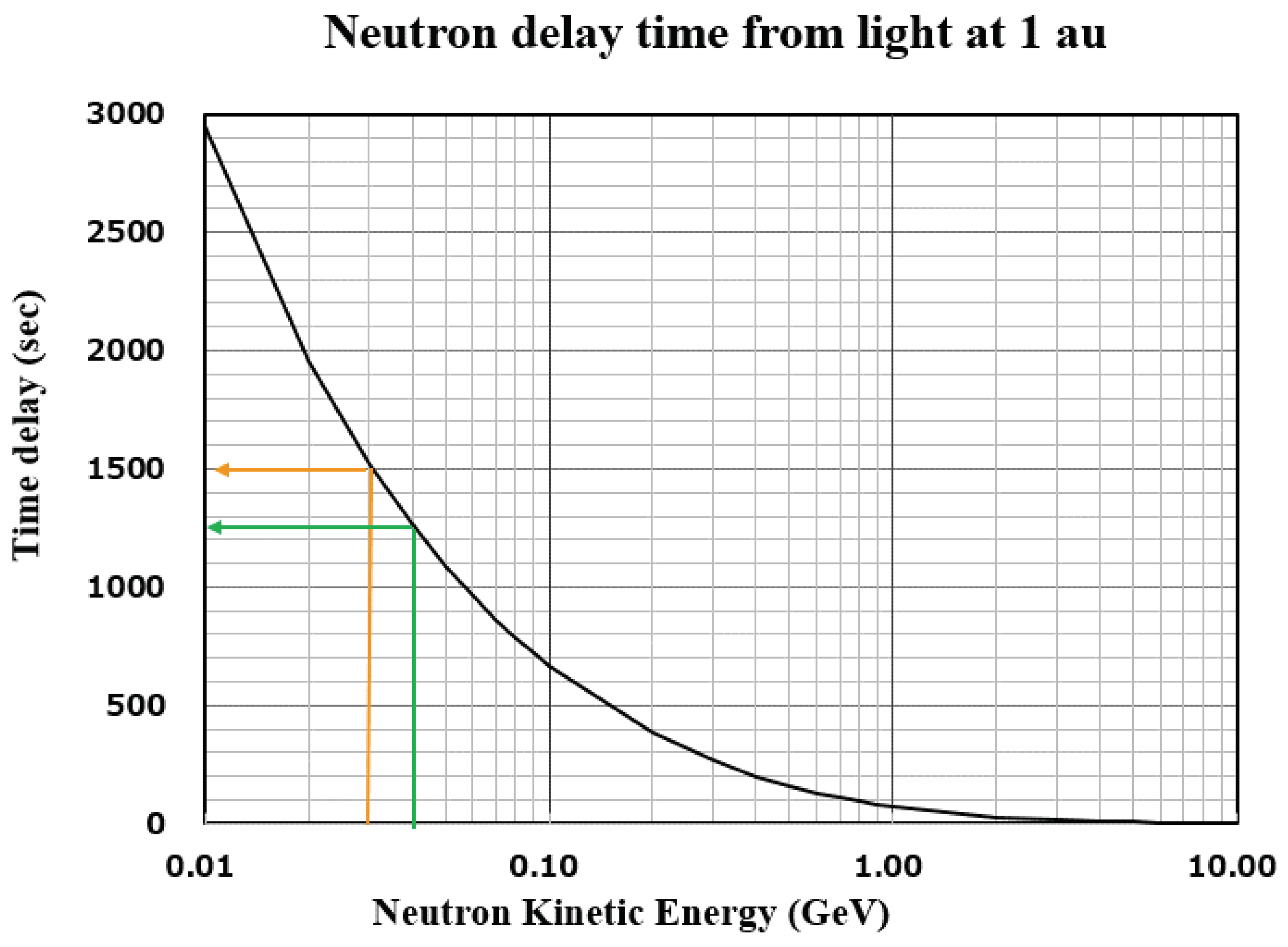
Figure 2.
The first solar neutron event recorded by the Gamma-Ray Spectrometer onboard Solar Maximum Mission on June 3rd 1982. From top to bottom, hard X-rays (56-199 keV), gamma-rays (4.1-6.4 MeV), and high energy particles over 25 MeV. The fourth curve presents the time profile of the neutron monitor located at Mt. Jungfraujoch (3,475 m). The Jungfrau detector recorded the enhancement induced by high-energy solar neutrons just after one minute later from the gamma-ray flash at 11:44 UT.
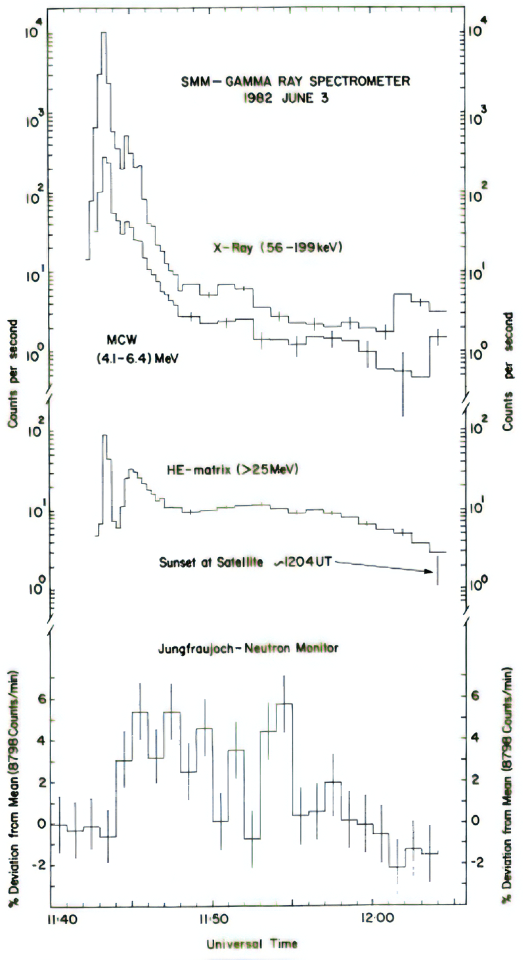
Figure 3.
A very intensive solar flare event was recorded at Climax on May 24, 1990. After one minute later, the sharp gamma-ray burst was recorded by the GRANAT detector, and the arrival of the neutron was recorded. The enhancement by the proton beam started after 18 minutes later from the arrival of neutrons.

Figure 4.
Examples of observations received at Mt. Norikura [12,13]. (a) One-minute value of the solar neutrons recorded on June 4, 1991. The left graph, from top to bottom, shows the time profile of the recorded event by 1 m2 neutron telescope, 36 m2 muon telescope, neutron monitor (12NM64), CGRO gamma-ray detector, and Nobeyama radio telescope. On the other hand, the right side graph (b) presents the solar neutron event recorded on June 6, 1991. From top to bottom, the data of 1 m2 neutron telescope, muon telescope, neutron monitor, Haleakala neutron monitor and Nobeyama radio telescope. It is interesting to know that the present solar neutron event was recorded over west of the Pacific area, Mt. Norikura and Mt. Haleakala of Hawaii.
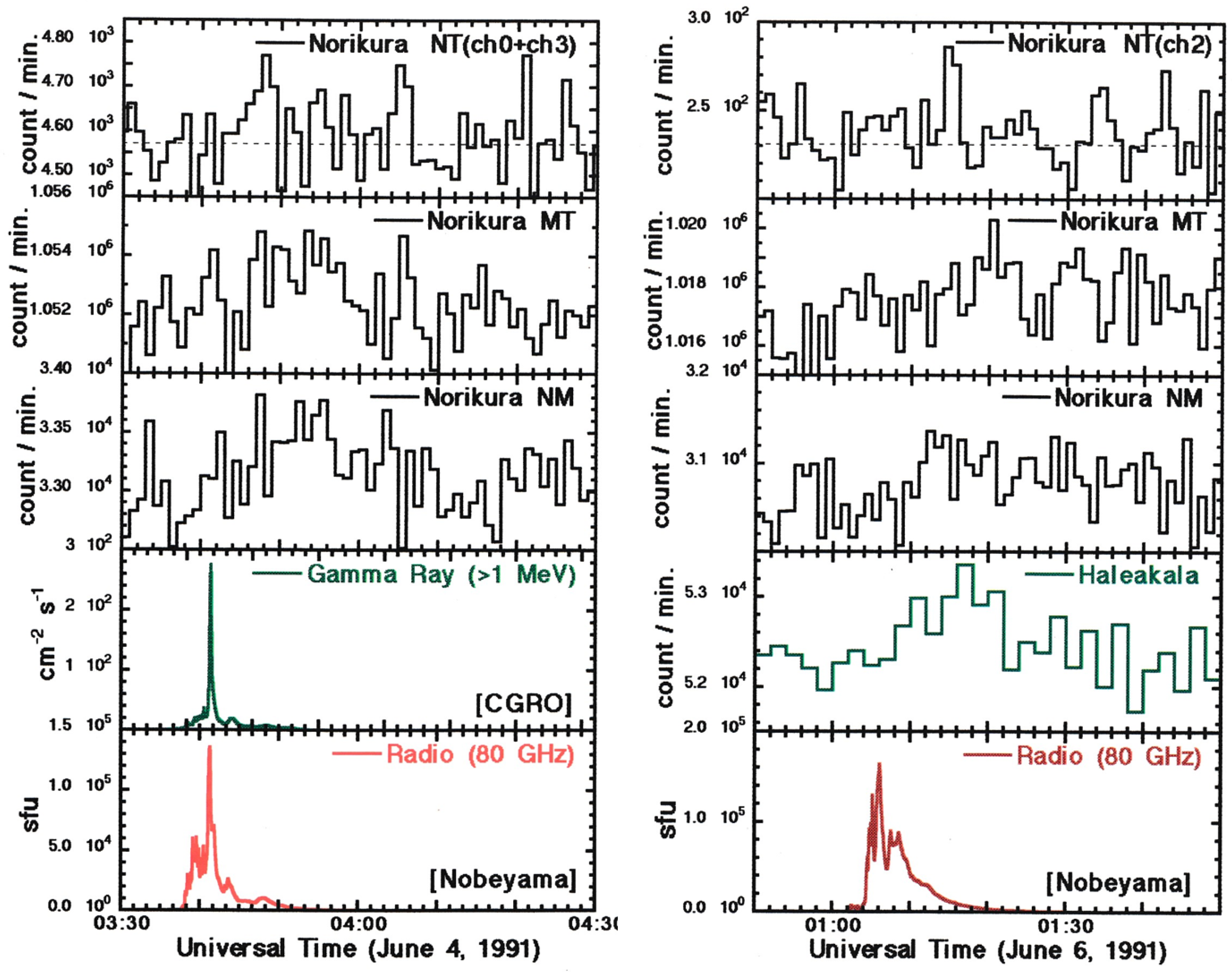
Figure 5.
(a) The left side pictures present the time profile of the solar neutron event recorded at Chacaltaya observatory in Bolivia (5,250 m). From top to bottom, these pictures present the time profile for the different threshold energy of the scintillator. The bottom picture shows the time profile recorded in the neutron monitor, while (b) represents the time profile recorded in the solar neutron telescope located at Mt. Sierra Negra, Mexico (4,600 m). The acceleration start time, 17:36:40 UT according to the record in the GEOTAIL hard-X-ray detector, is presented by the green dashed ine in each figure.
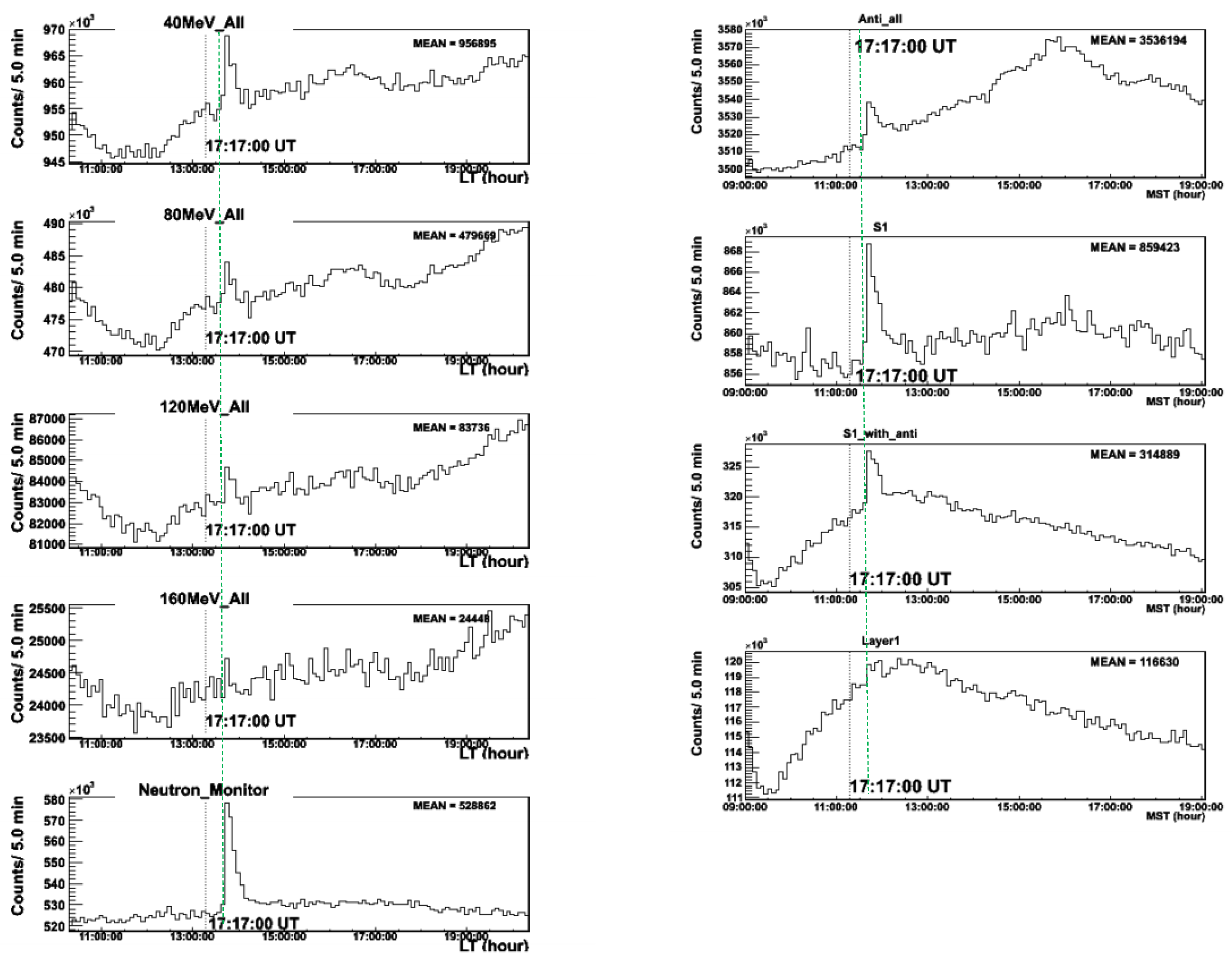
Figure 6.
The time profile recorded in the solar neutron telescope at Mt. Sierra Negra on November 7, 2004. The GOES start time of the flare at 15:42:00 UT is shown by the vertical dotted line, while the horizontal green line with arrows indicates the excess time over the average counting rate. The top picture presents the anti-counter counting rate, while the bottom picture indicates the S1 channel. The S1 channel is required in case it triggers the signal to the threshold energy over 30 MeV. The green arrow indicates the time span of excess as 55 minutes.
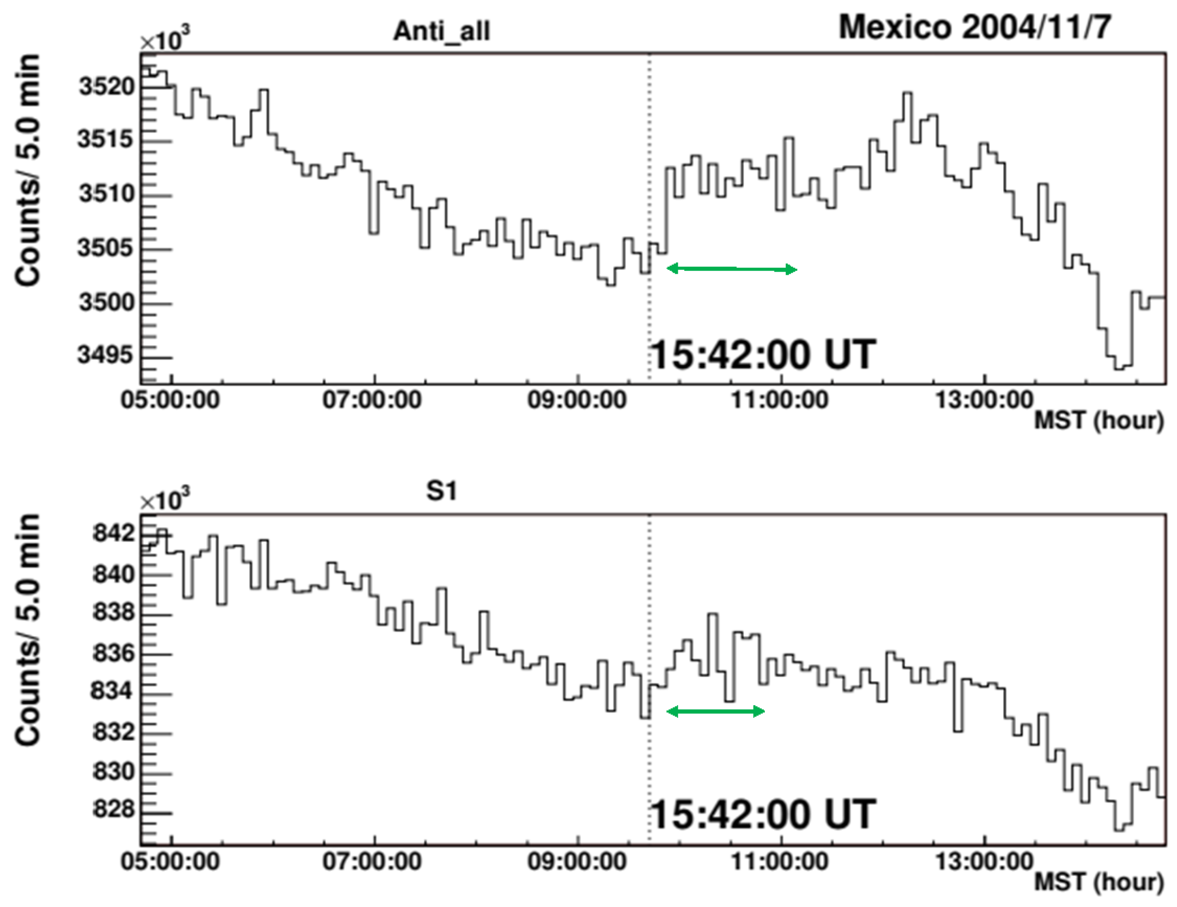
Figure 7.
Photograph of the neutron monitor located at Mt. Norikura cosmic ray observatory (2,778 m) (left) and the BF3 counter (Chalk River neutron counter) (right).
Figure 7.
Photograph of the neutron monitor located at Mt. Norikura cosmic ray observatory (2,778 m) (left) and the BF3 counter (Chalk River neutron counter) (right).
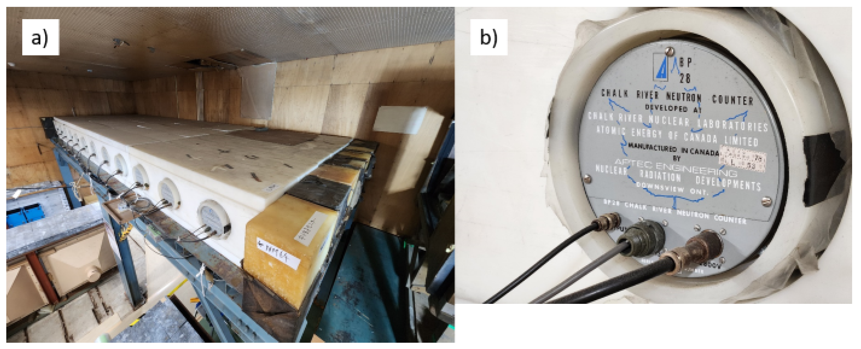
Figure 8.
Solar Neutron Detector constructed at Chacaltaya cosmic ray observatory (5,250 m), (a) presents the 4 blocks of plastic scintillator, each has a dimension of 1 m2 and inside 40 cm thick plastic scintillator was installed. Photograph (b) indicates the anti-counter that surrounds the 4 blocks of plastic scintillator for the use of identification of charged particle entrance or neutral particle entrance.
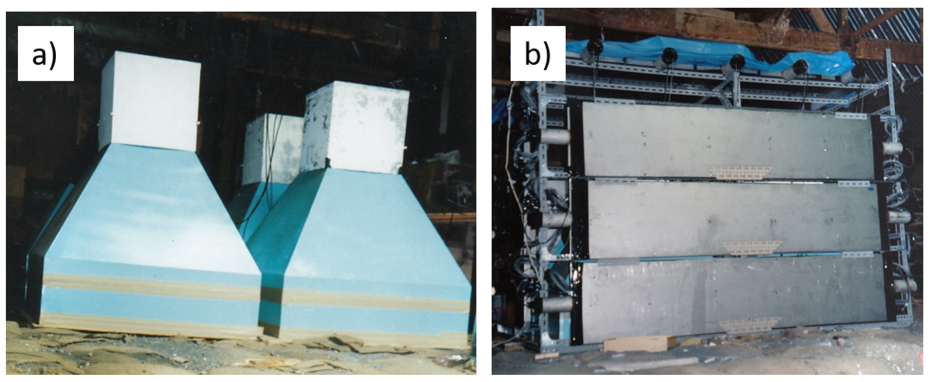
Figure 9.
These photographs show just before the assembly of the solar neutron telescope at Mt. Sierra Negra (4,600 m). Photo (a) presents the thick plastic scintillator inside one module of the detector, photo (b) presents the mounting of the proportional counter for the use of an anti-counter on the top and side of the central thick plastic detector with an area of 4 m2.
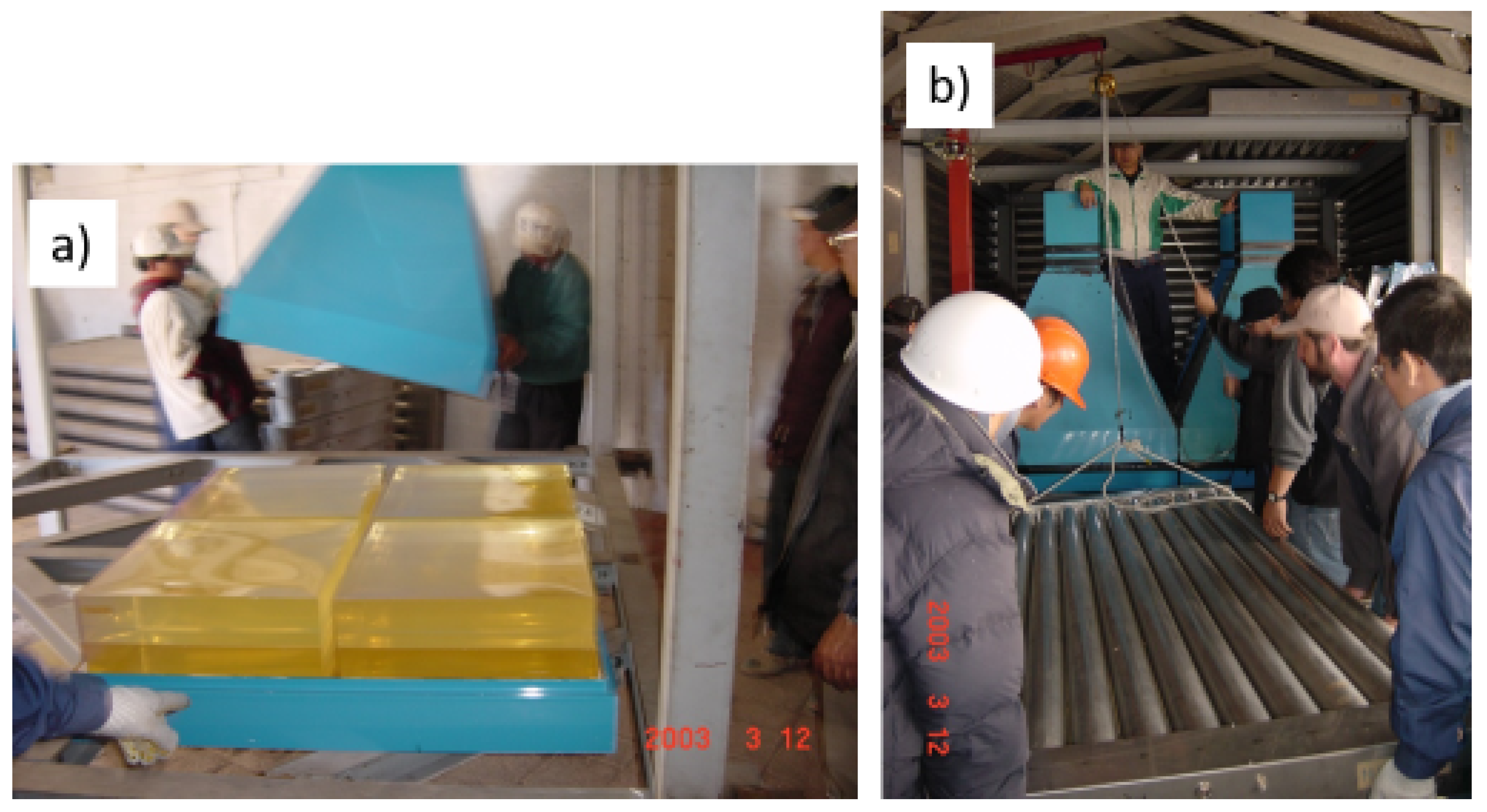
Figure 10.
One minute value of GOES X-ray data on November 7, 2014, red and blue curve, corresponding to the X-ray wave-length as 1.0-8.0 Å(red) and 0.5-4.0 Å, respectively. The green curve indicates the derivative of the increase of the short band X-rays (0.5-4.0 Å). Three peaks of green plots can be recognized in the figure that corresponds to the 3-step increase of the flare from C-class to M-class and X2-class. The blue arrow indicates the start time of acceleration of ions into high-energy in this flare, i.e.,15:46:00 UT.
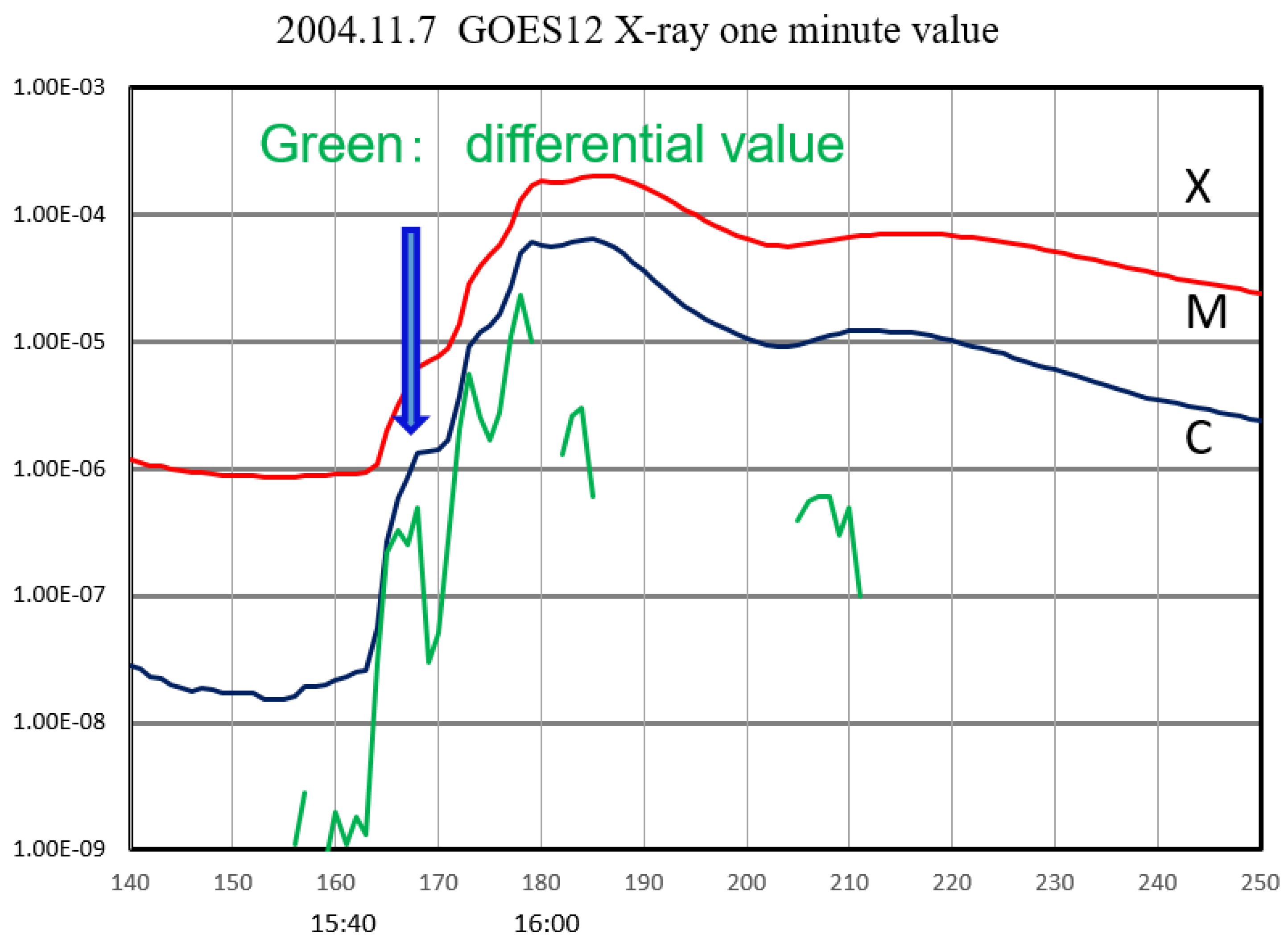
Figure 11.
The time profile of the November 7, 2004 event recorded by the solar neutron detector at Mt. Chacaltaya with the channel of the threshold energy higher than 40 MeV. The number indicated in the figure, on the time of ➀, corresponds to the direction of arrival of the Parker field. The time, ➂ coincides with the arrival time of Forbush Decrease to the vicinity of the Earth. The time of ➁ just corresponds to the solar flare time. The duration of increase during 20 minutes is just expected from the assumption; if solar neutrons were produced instantaneously at the solar surface, neutrons with energy higher than 40 MeV must arrive within 20 minutes (see the green arrow in Figure 1).
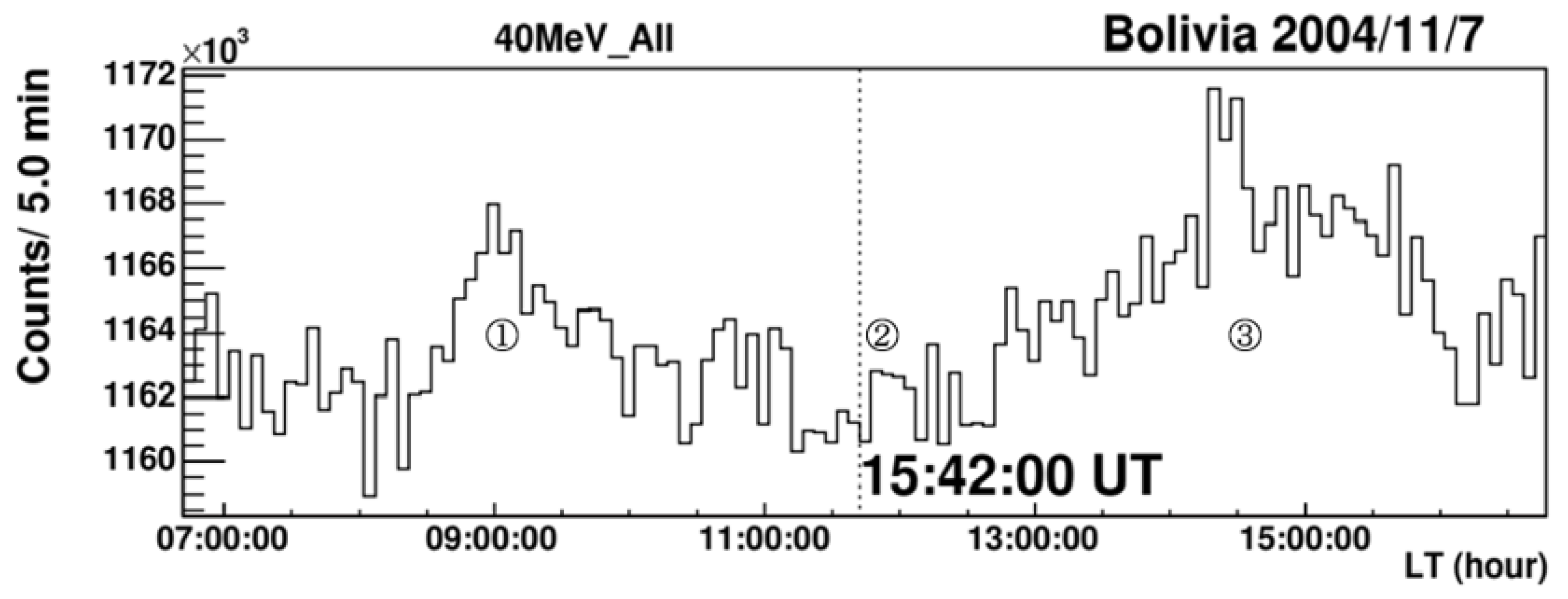
Figure 12.
The time profile of the same event recorded by the Chacaltaya solar neutron detector, but the threshold channels were higher than 120 MeV and 160 MeV. Although the statistical significances were weaker than that of 40 MeV, however, we can recognize 3 level enhancements.
Figure 12.
The time profile of the same event recorded by the Chacaltaya solar neutron detector, but the threshold channels were higher than 120 MeV and 160 MeV. Although the statistical significances were weaker than that of 40 MeV, however, we can recognize 3 level enhancements.
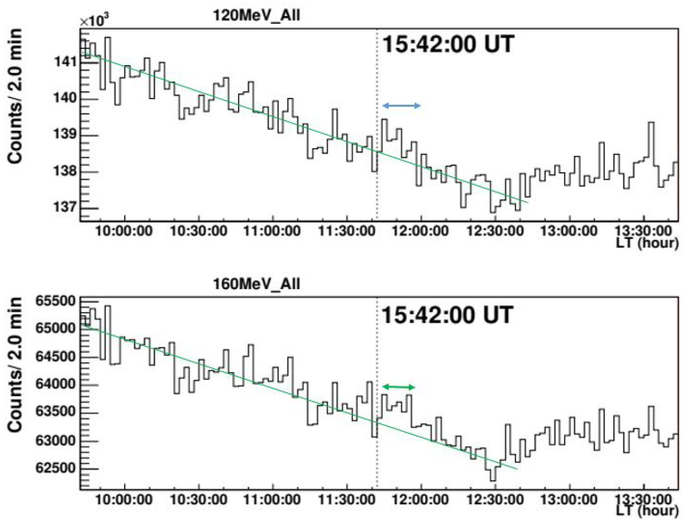
Figure 13.
From the one-minute time profile recorded by the Chacaltaya neutron detector, assuming the instantaneous production of those neutrons at the Sun, the differential energy spectrum can be deduced. This figure was deduced by just the number of events () divided by the energy bin ().
Figure 13.
From the one-minute time profile recorded by the Chacaltaya neutron detector, assuming the instantaneous production of those neutrons at the Sun, the differential energy spectrum can be deduced. This figure was deduced by just the number of events () divided by the energy bin ().
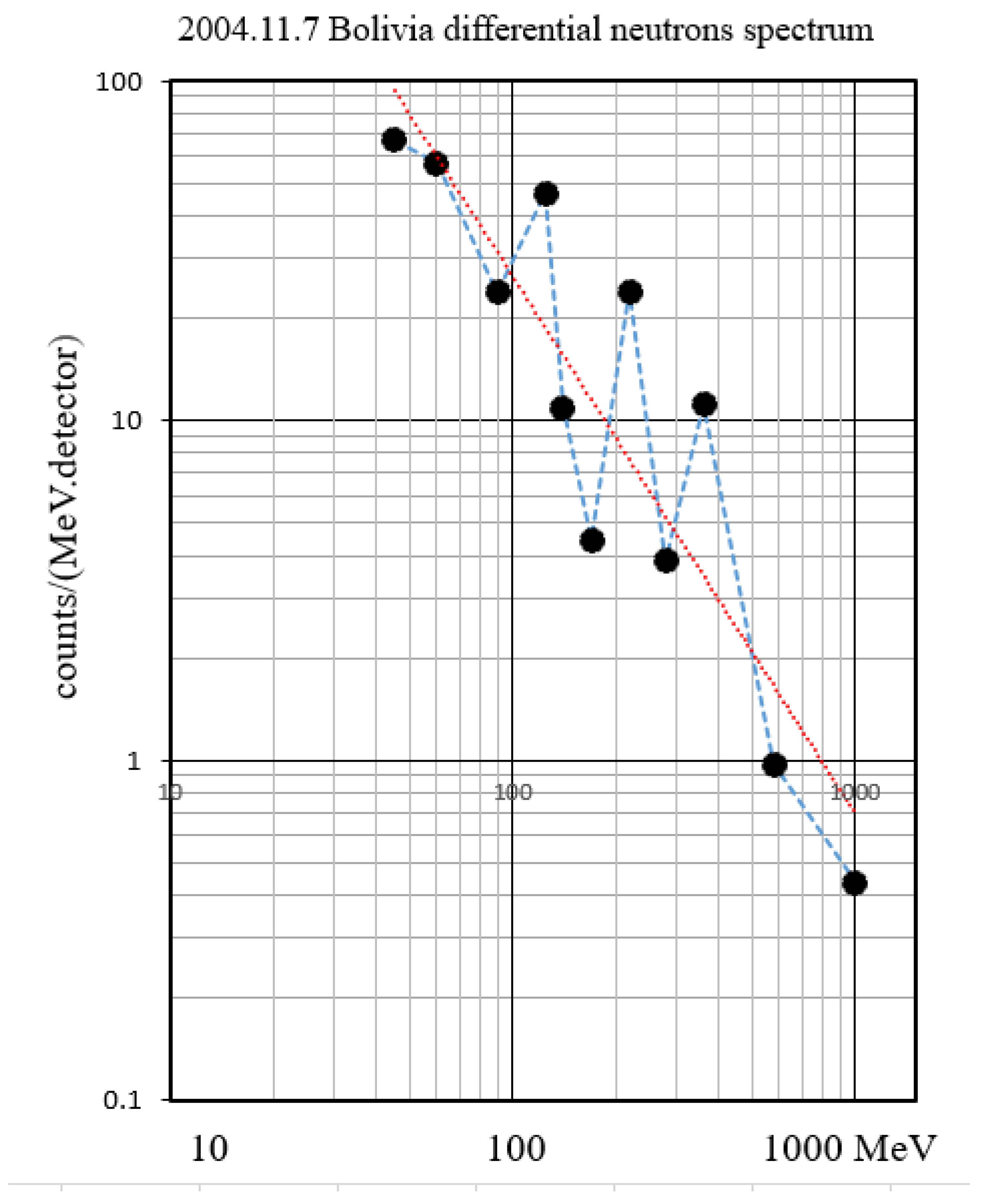
Figure 14.
The differential energy spectrum of solar neutrons detected at Mt. Chacaltaya on November 7, 2004. Since Figure 13 does not include the energy dependency of the detection efficiency, in this picture, they are involved. This figure was made after dividing the flux of Figure 13 by the energy dependence of the detection efficiency for solar neutrons.
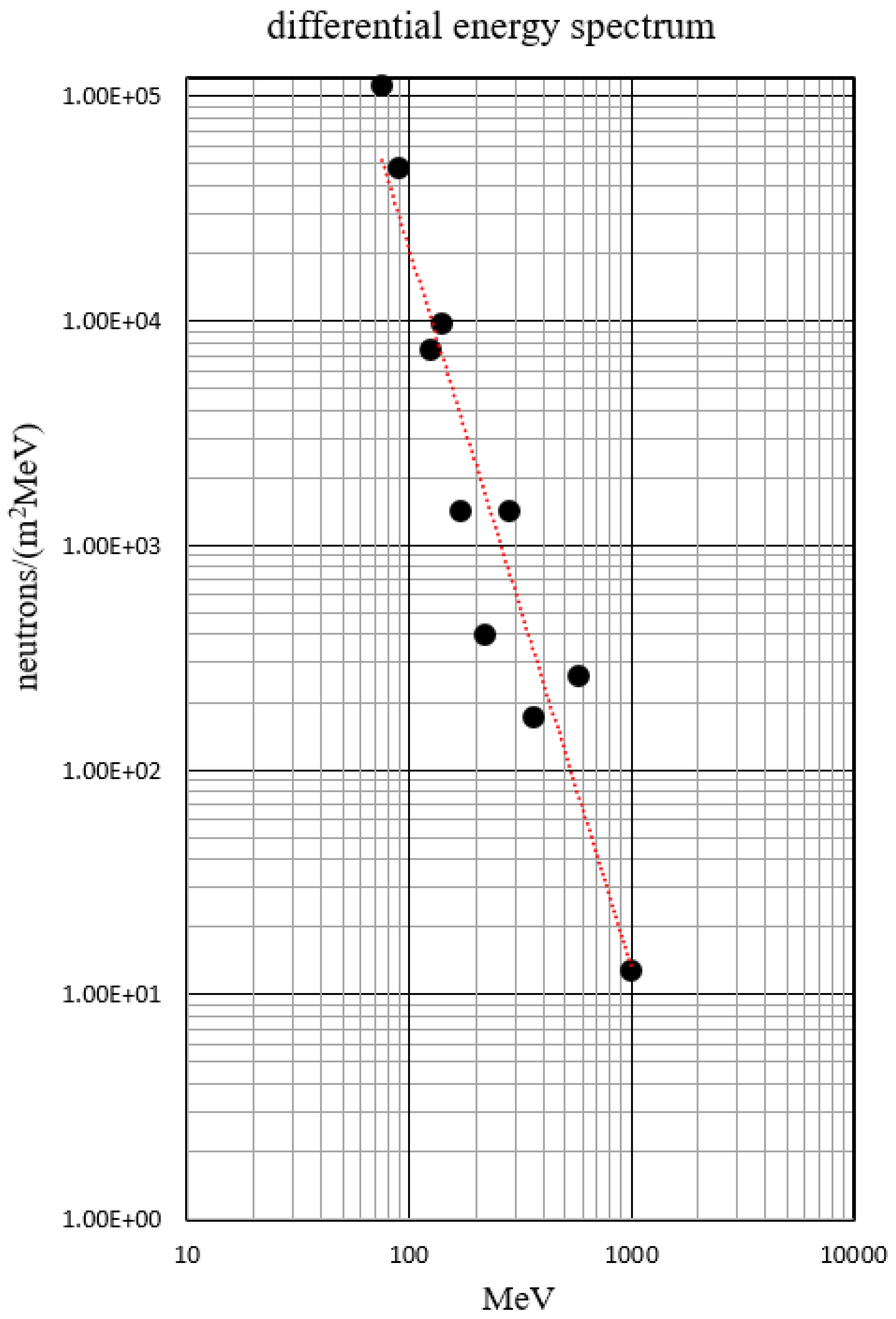
Figure 15.
The integral energy spectrum of the November 7, 2004 solar event. The expected flux beyond 10 GeV is also plotted in the energy region of 1-10 GeV. The flux represents per unit area (/m2) at the top of the atmosphere.
Figure 15.
The integral energy spectrum of the November 7, 2004 solar event. The expected flux beyond 10 GeV is also plotted in the energy region of 1-10 GeV. The flux represents per unit area (/m2) at the top of the atmosphere.
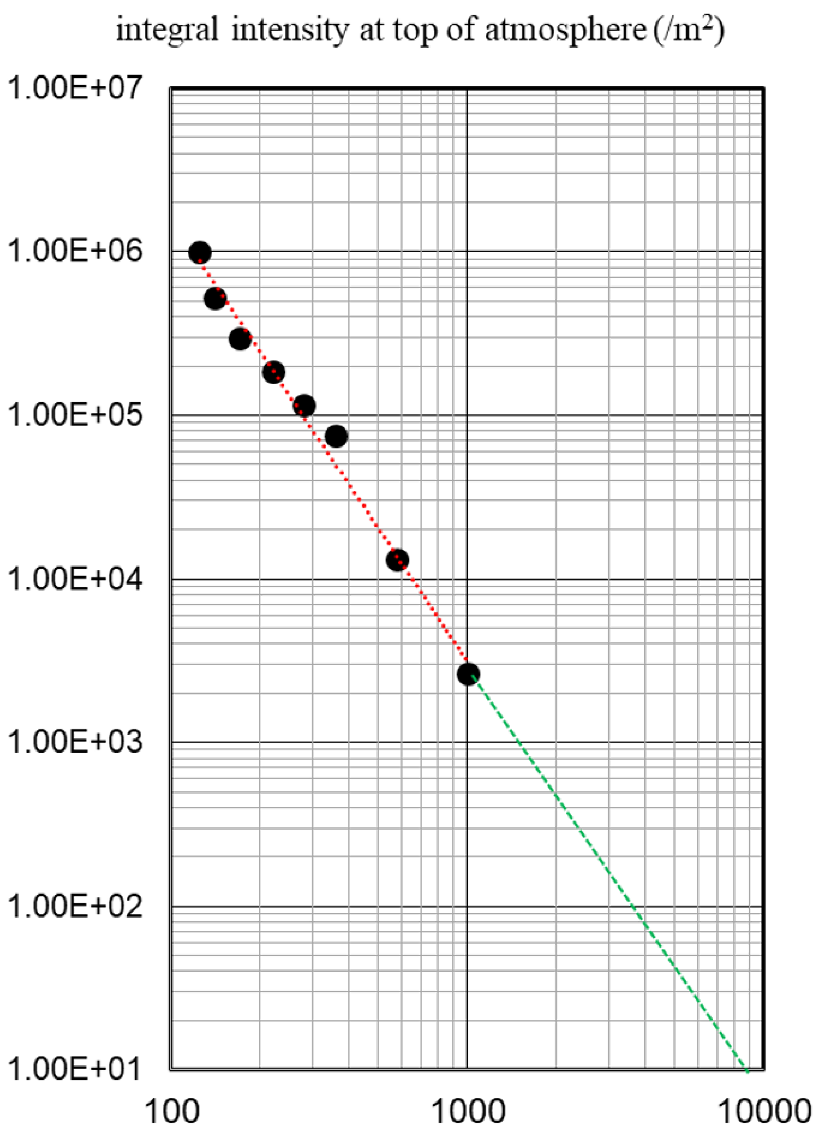
Figure 16.
The atmospheric depth when solar neutrons pass through the atmosphere. This picture clearly shows that the Chacaltaya observatory was located at the best condition for detecting solar neutrons on November 7, 2004. The difference in the atmospheric thickness between Mt. Sierra Negra (768 g/cm2) and Mt. Chacaltaya, Bolivia (551 g/cm2) is 217 g/cm2. The yellow area represents when we take into account the large angle scattering of solar neutrons at the top of the atmosphere, and blue does not include such an effect.
Figure 17.
The penetration efficiency of protons into the magnetosphere over Mexico around 16 local times. From top to bottom, the open square represents total penetration efficiency. This corresponds to the case that protons can enter not only the dayside but also from the night side (tail side of the magnetosphere). On the other hand, open triangles show the cases when protons enter from the day side. Open circles represent protons that enter within 40 degrees from the vertical 20 km above Mt. Sierra Negra, while closed circles represent the cases when protons enter into the air within 20 degrees from the vertical. In the latter case, protons are less attenuated.
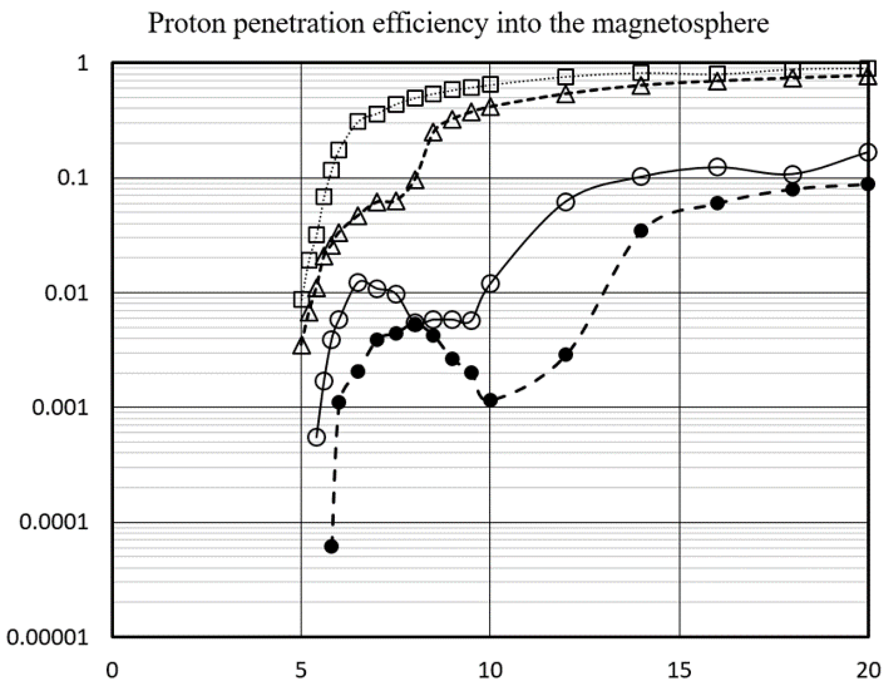
Figure 18.
The transition curve of the secondary particles when protons with energy 7 GeV enter in the air. The red dots correspond to gamma-rays with an energy higher than 30 MeV, while the blue dots represent the attenuation of the secondary neutrons in the air with an energy higher than 30 MeV. The vertical gap at 570 g/cm2 corresponds to the location of a 5 mm thick lead plate over the anti-counter of the Mt. Sierra Negra detector. The calculation was made by GEANT4 software.
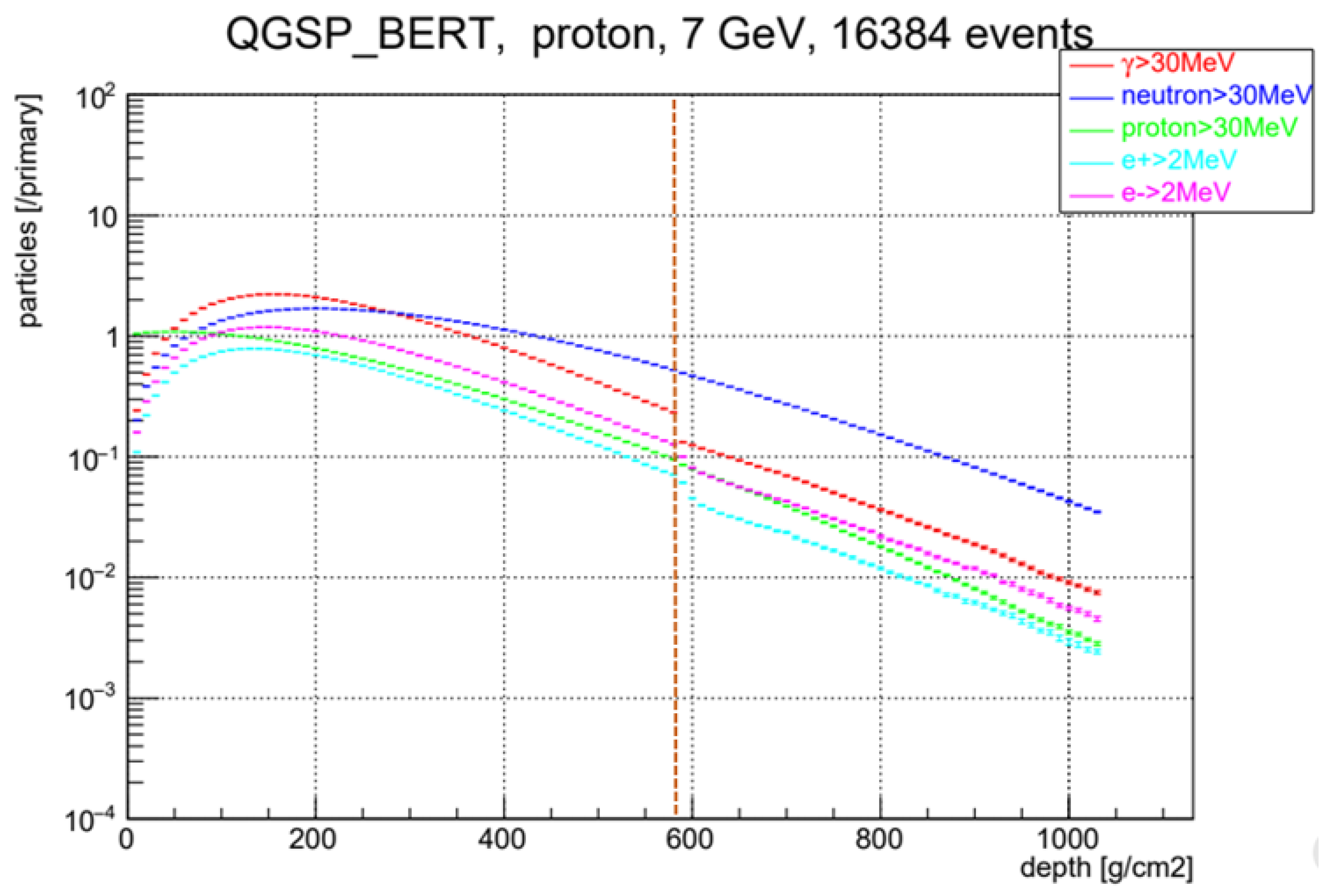
Figure 19.
The detection efficiencies of incident protons with the energy of 4 GeV and 6 GeV are shown as a function of the incident angle on the top of the atmosphere. Open and closed circles correspond to neutrons with an energy higher than 32 MeV for the incident energy 4 GeV (○) and 6 GeV (●), respectively. The triangles correspond to the gamma-rays with an energy higher than 2 MeV for the incident energy of protons of 4 GeV (△) and 6 GeV (∆), respectively. Note that the threshold energy is set at 2 MeV not 30 MeV.
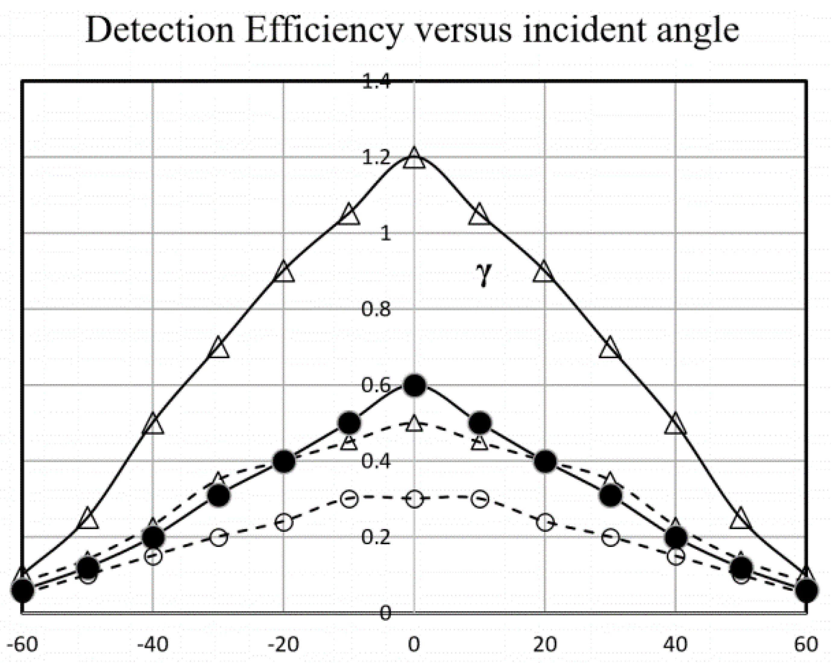
Figure 20.
The space environment observed by the GOES 12 satellite on the 7th and 8th of November 2004. From top to bottom, the panel shows solar X-ray intensity, charged particles and magnetic field, respectively, while the bottom panel shows the cosmic-ray intensity measured by the neutron monitor located at McMurdo. The sudden change of the magnetic field and cosmic-ray intensity around 18:30 UT tells an arrival of Forbush Decrease that coincides with the M9.3 flare on November 6th at 00:34 UT.

Figure 21.
The two-day map of the solar space environment measured by the Nagoya University UHF radio telescope. The solar wind group of Nagoya University uses the radio telescope that has a sensitivity of 327 MHz. The telescope measures the scintillation of radio stars induced by the solar wind. By this method, they measure the nearly 3-dimensional distribution of the solar wind. (a) the left side figure shows the space distribution of the solar wind during November 7, 2014, 22:00 UT to November 8, 07:00 UT, while (b) shows the same distribution during November 8, 22:00 UT to November 9, 07:00 UT. On the slide (b), the CME’s two-arm structure clearly recognises that was produced at the same time as the X2.0 solar flare appeared on 16:00 UT of November 7, 2014.
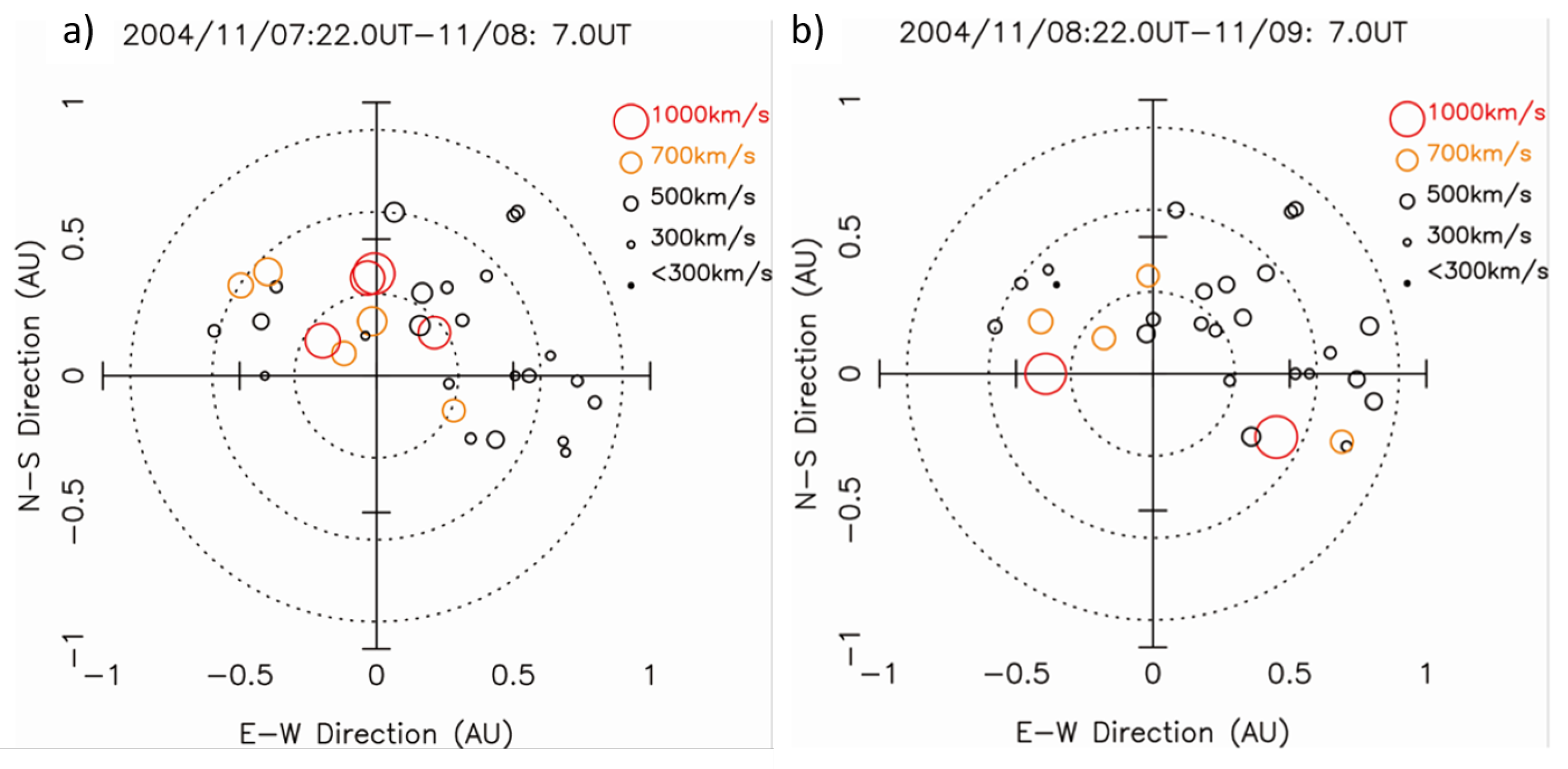
Figure 22.
The solar space environment around 16:00 UT on November 7, 2014, is pictorially presented. Distinctive features are recognized: the two CME ropes, here named CME1 and CME2, and the CME1 did not pass over the Earth at 16:00 UT. It passed at 18:30 UT. Therefore, in front of the CME1, still some space with B=10 nT remained. The distance between the front of CME1 and the Magnetopause is estimated as 0.066 au or m.
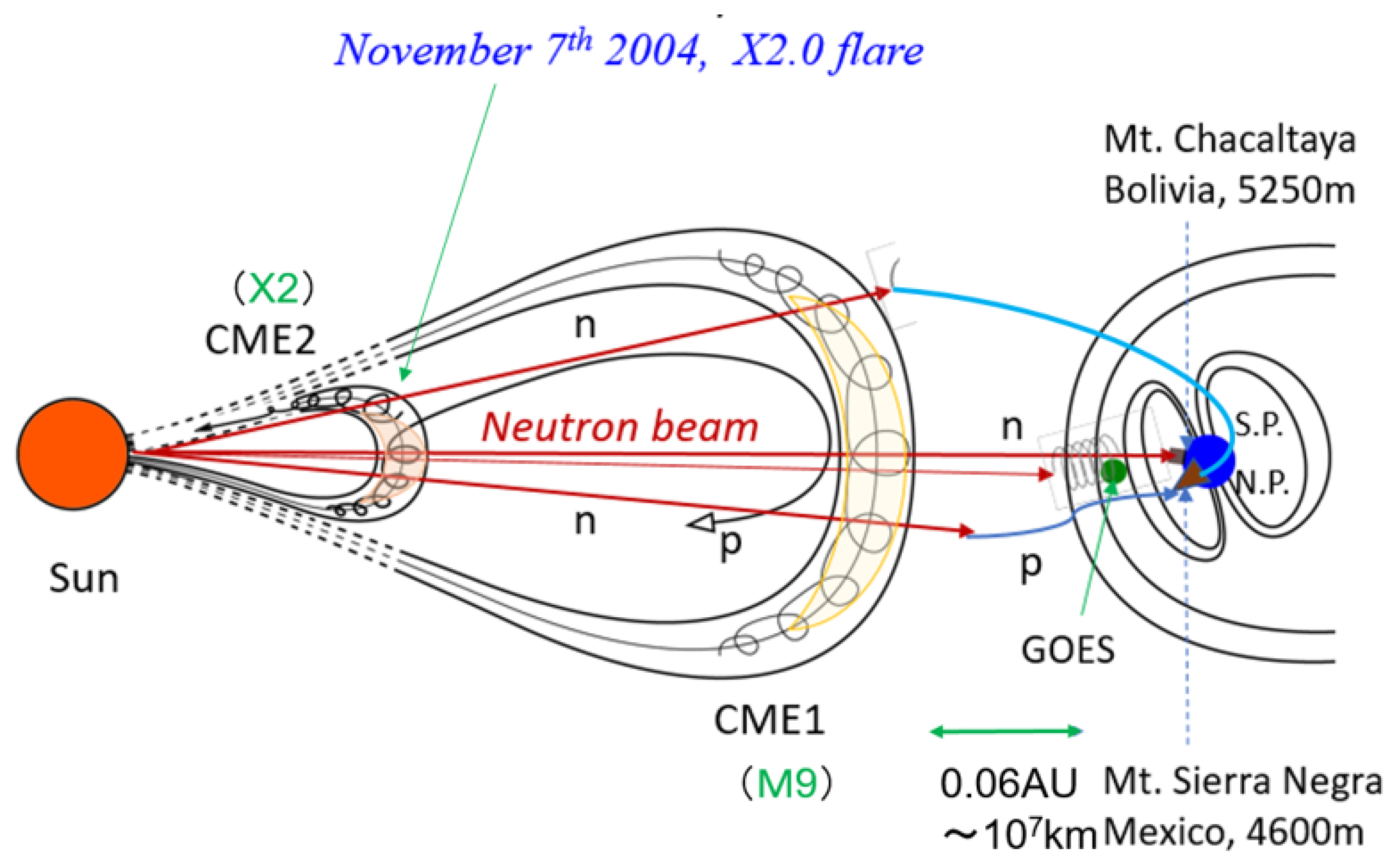
Figure 23.
The expected flux of solar neurons in a higher energy range between = 1 and 10 GeV. The red, orange and green plots correspond to the different powers of the integral spectra () with = 2.75, 3.75 and 4.75, respectively. The point at 1 GeV is normalized at the observation value of the Chacaltaya neutron detector (converted to the flux at the top of the atmosphere). The dashed lines represent the flux after taking into account the decay effect in the flight of 0.066au. The blue dotted line below shows the decay probability of neutrons during the flight at the distance of 0.066 au. The vertical line at 5GeV indicates the lower detection limit of SNDPs.
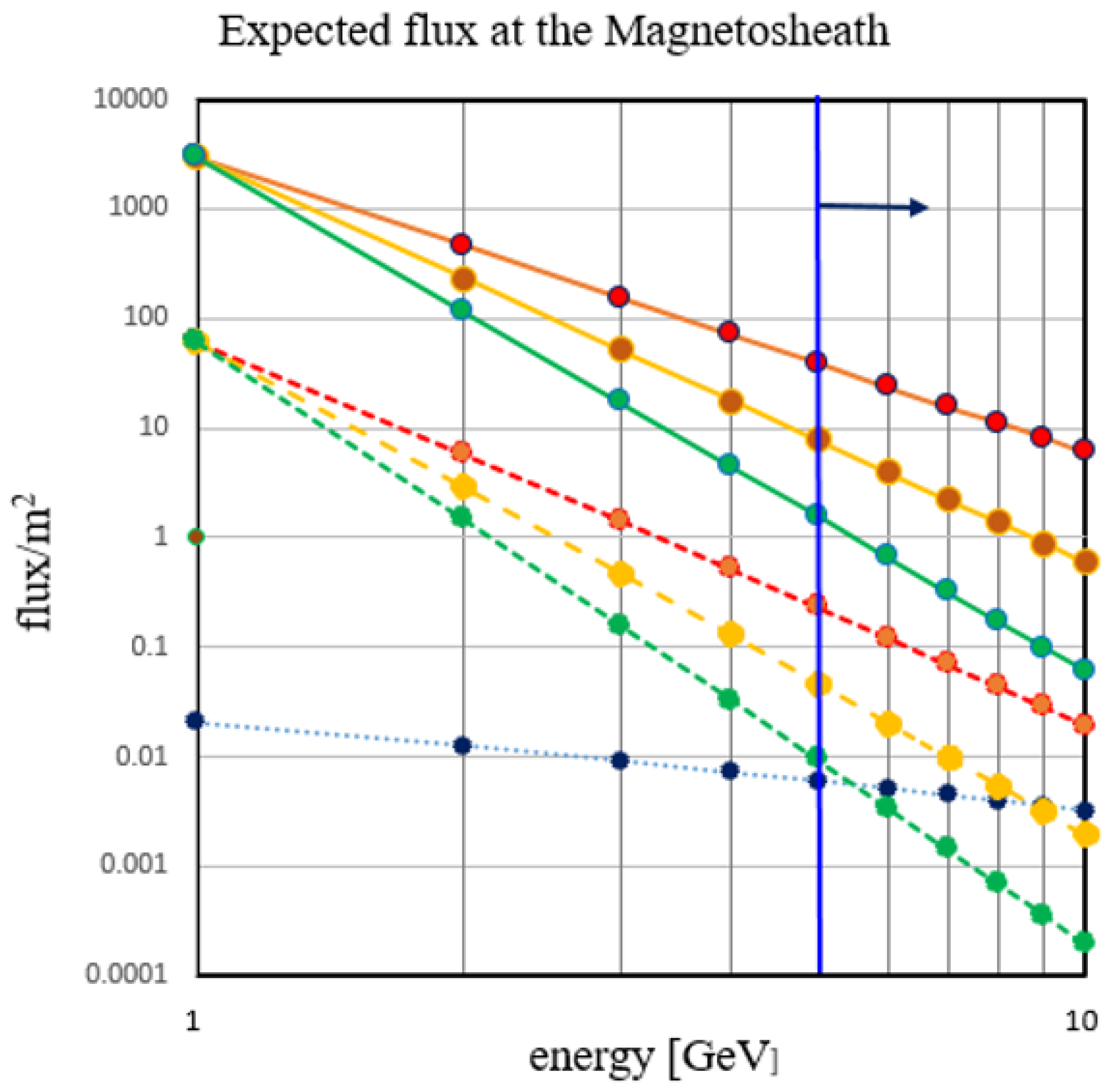
Figure 24.
The arrival points at 8 of the anti-protons ejected from 20 km above Mt. Sierra Negra are presented. The arrival points are plotted on the X-Y plane of the GSE coordinate, where the positive X directs the Sun. The arrival points in the night area are shown by the blue points. We notice that only a few trajectories among 32,761 shots arrived at 8 at low energy. However, when the energy of anti-protons increases from 4.7 GeV (left), 5 GeV (middle) to 6 GeV (right), the arrival points increase.
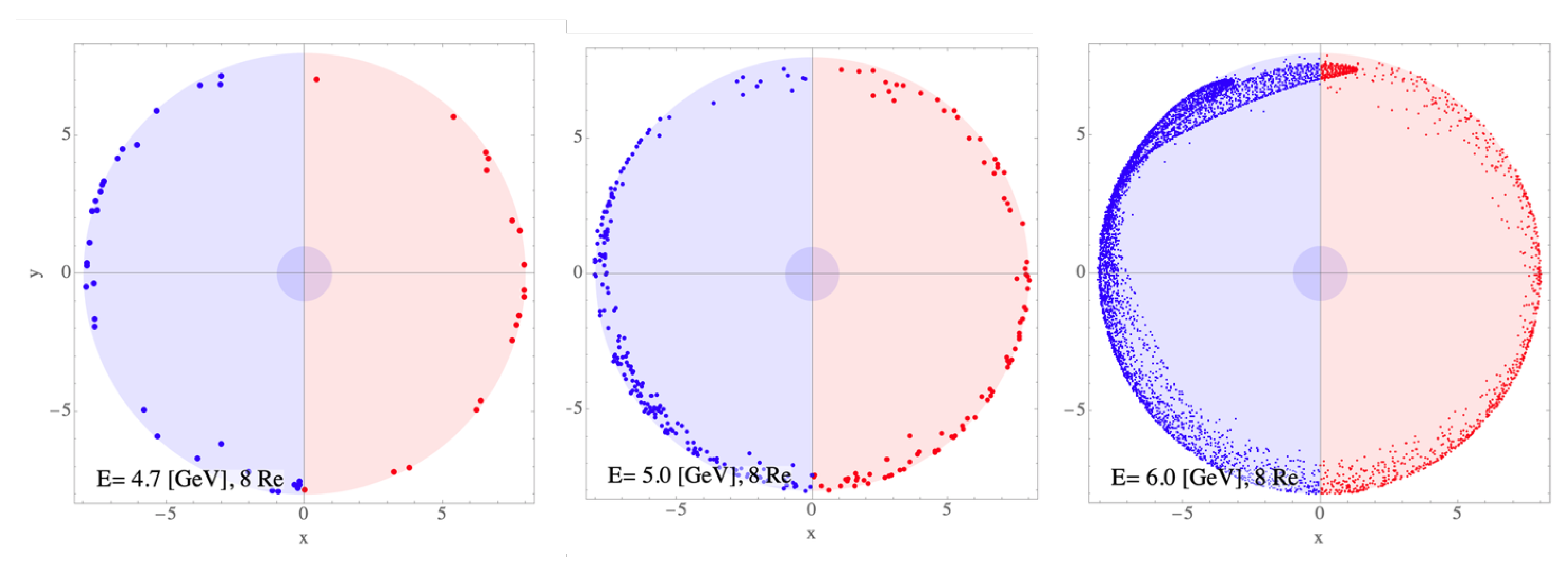
Figure 25.
The momentum distribution of anti-protons at 8 is shown on the diagram. The plot is made to the momentum that satisfies the conditions (1) , (2) the emission angle of anti-protons is less than 40∘ from the vertical, and (3) . In the plot, the thin blue line represents 50∘ from the axis, and the blue arrow indicates the crossing angle of the Parker field to the magnetosphere. The solar neutron decay protons are transported by the Parker field. Therefore, the matching condition of the two streams, the Parker field and anti-proton outgoing direction is the key point for the smooth connection of the SNDP in the magnetosphere.
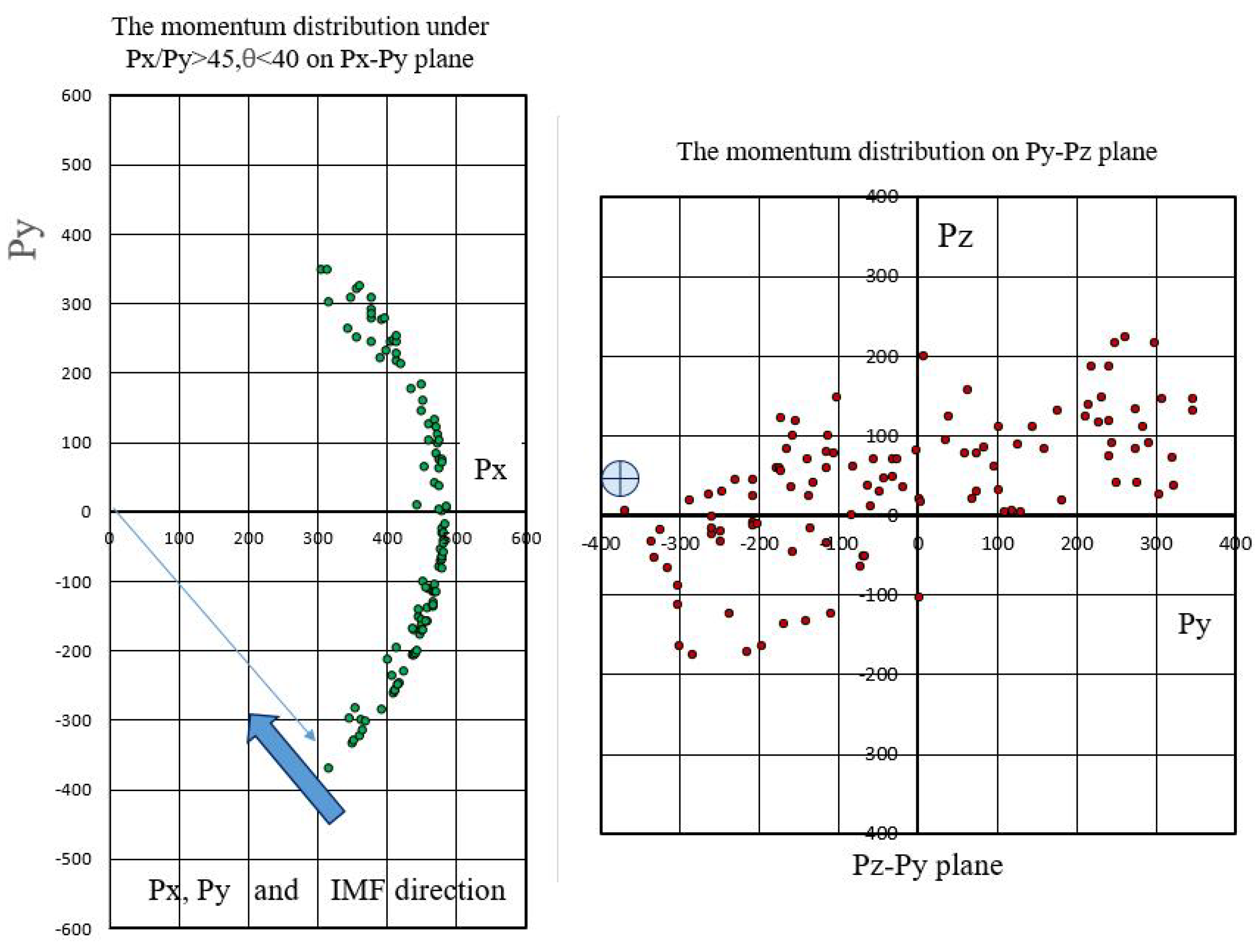
Figure 26.
Measurement of the solar wind velocity by the ACE plasma detector. The ACE satellite is situated at Lagrangian point L1. The distance to the L1 point from the Earth is km or 0.01 au. The solar wind with the velocity of 400 km/s arrived at the Earth after one hour later. So the solar wind velocity around 14:00∼15:00 UT observed by the ACE satellite presents the solar wind velocity around 16:00 UT of the Earth.
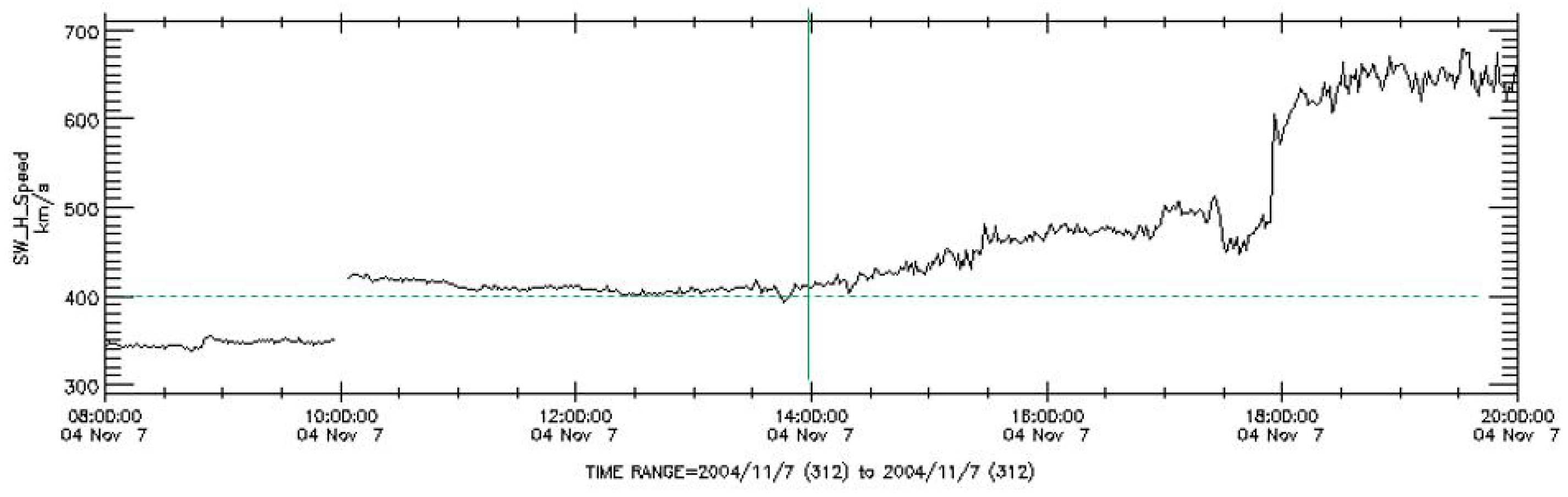
Figure 27.
The one minute value of the counting rate of the Oulu neutron monitor 9NM64 between 15:00 and 17:00 UT on November 7, 2004. Around 16:00 UT, a 5 level enhancement can be recognized.
Figure 27.
The one minute value of the counting rate of the Oulu neutron monitor 9NM64 between 15:00 and 17:00 UT on November 7, 2004. Around 16:00 UT, a 5 level enhancement can be recognized.
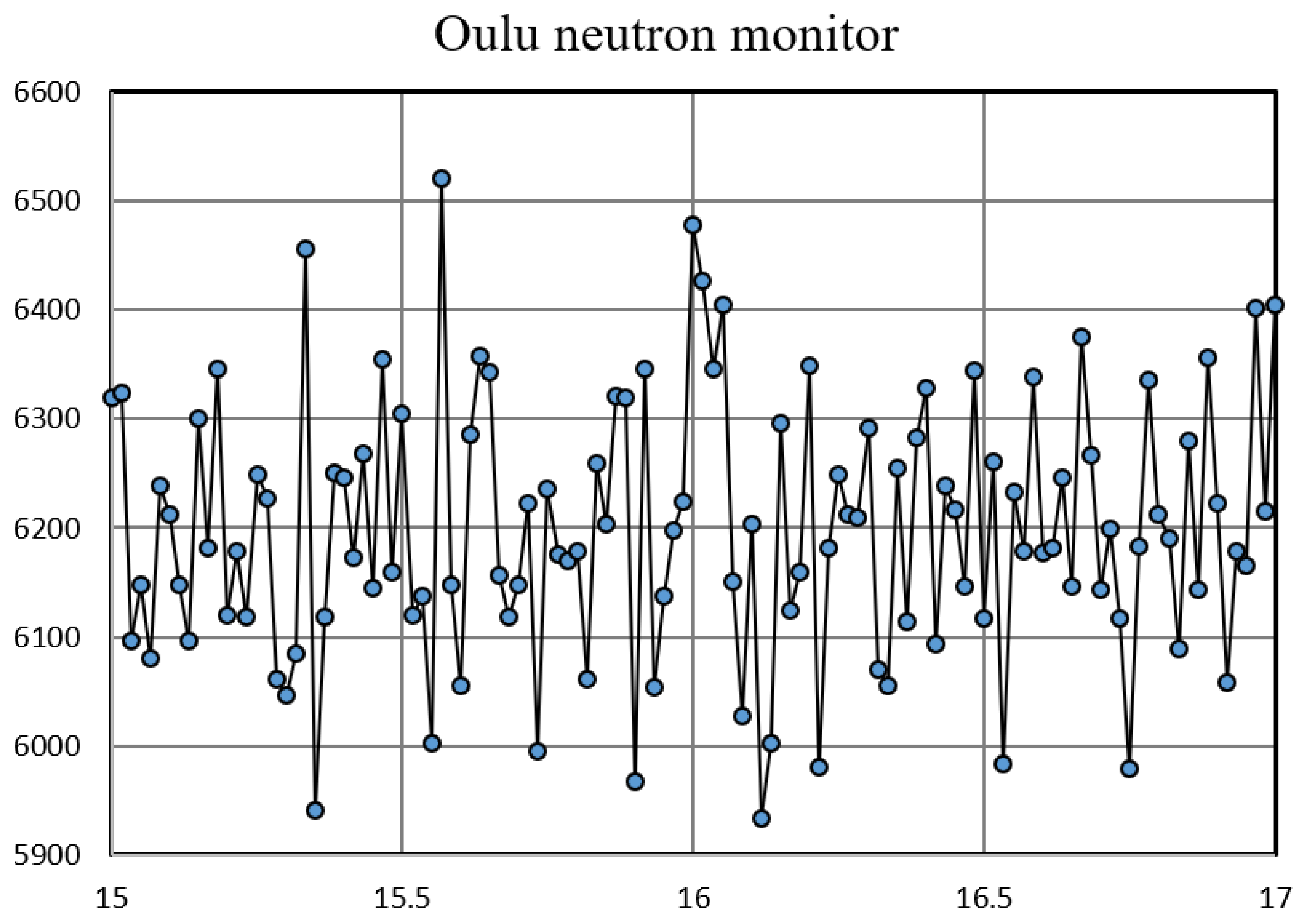
Figure 28.
The transition curve of secondary particles in the atmosphere is presented as a function of the thickness of the atmosphere. The curve presents the case when proton with energy of 4 GeV hits at the top of the atmosphere. At the ground level (1000 g/cm2), about the incident proton signal will be reduced down to 1/50, however, they will be recorded by the neutron monitor. The curve is made by the GEANT4 simulation.
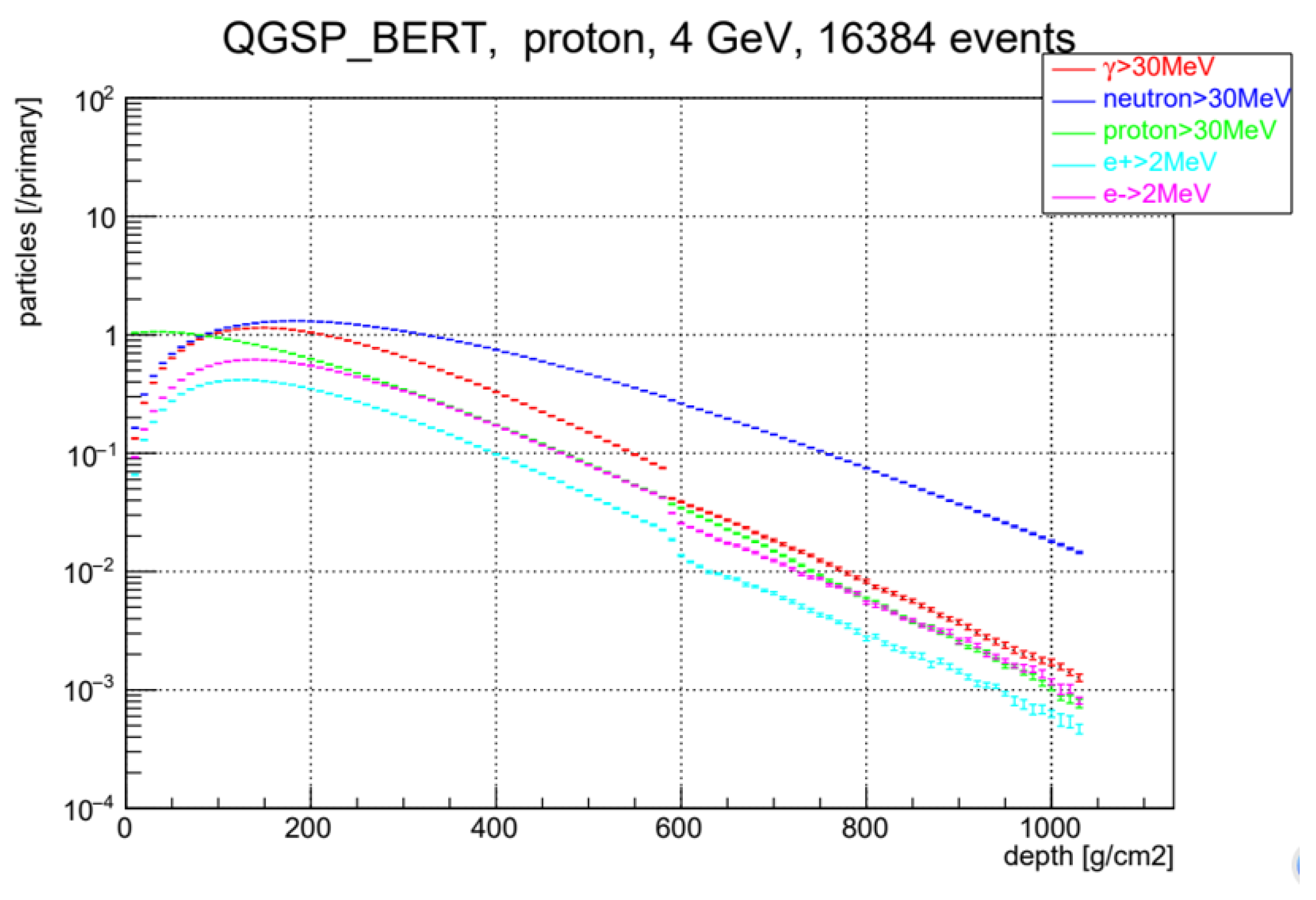
Figure 29.
A schematic trajectory of neutron decay protons to Oulu station is presented on the GSE coordinate. The X-direction looks toward the solar direction, while the positive z-direction corresponds to the North pole. The small blue area in the night zone represents the allowed region for solar neutron decay protons (SNDP) at 15 . The incident energy of solar neutrons is set at 0.4 GeV. At 10:50 UT, the solar direction was just on the horizon.
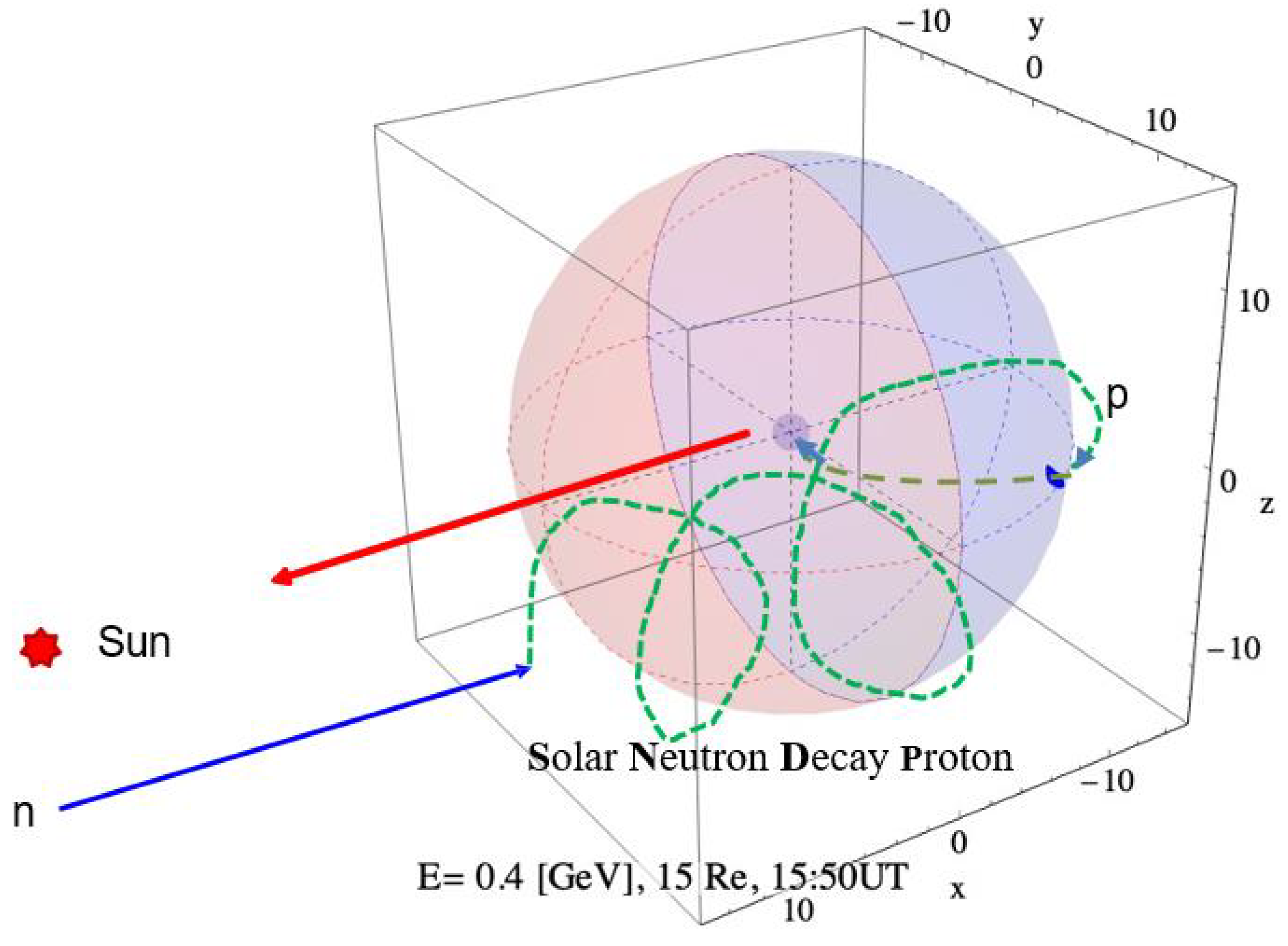
Figure 30.
The top figure shows the time profile of the counting rate of the proton channel of GOES satellites; GOES 10 (black) and GOES 12 (blue). On November 7, 2004, the GOES 10 was located at 75∘E while GOES 12 was situated over 135∘E. GOES 10 faced the Sun directly (11 am local time) and it has succeeded to detect a signal of the arrival of solar neutrons, while for GOES 12, the flare time was at early morning (7 am local time), so the signal of solar neutrons was not recorded. The bottom figure shows the counting rate of higer 10 MeV channel of GOES 11 satellite. The excess continued for 10 minutes (the red arrow) in coincidence with X2.0 solar falare. The local time of GOES 11 satellite was 9 am, and neutrons were able to enter the proton counter of GOES 11 satellite, then might be converted to protons. The peak at 18:30 (green arrow) might be induced by Forbush Decrese.
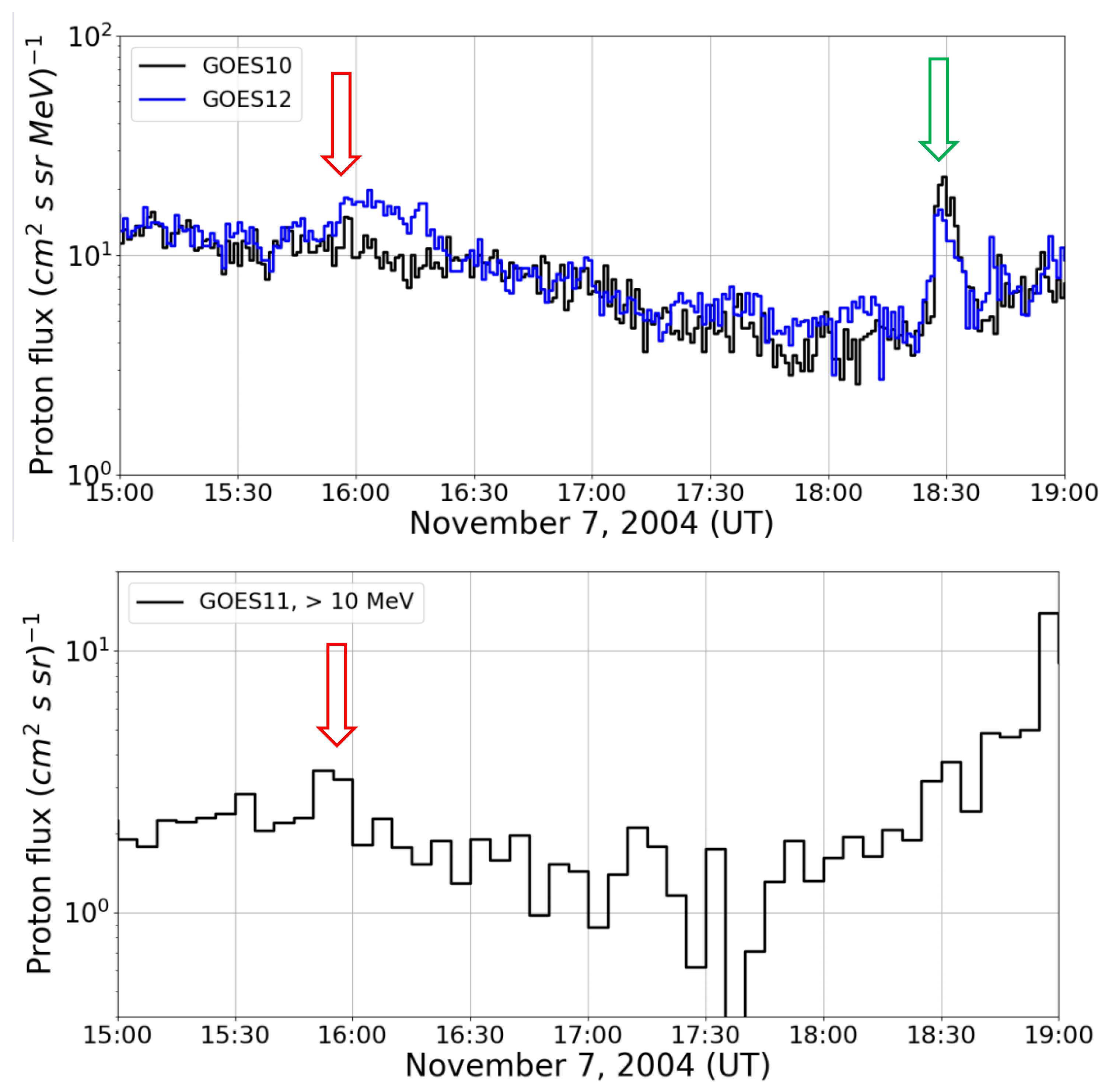
Figure 31.
The solar surface on November 7, 2004 taken by the SOHO telescope with 195 nm wave length. The left side photo shows the solar surface at 15:36:11 UT just before the start time of GOES X-ray flare (15:42 UT). The right side slide presents at 15:48:11 UT just one minutes later of the ion acceleration time. Particles may be accelerated at the brightest point of the arch (X, Y)=(260”,100”) arc sec in the photo indicated by the white arrow.
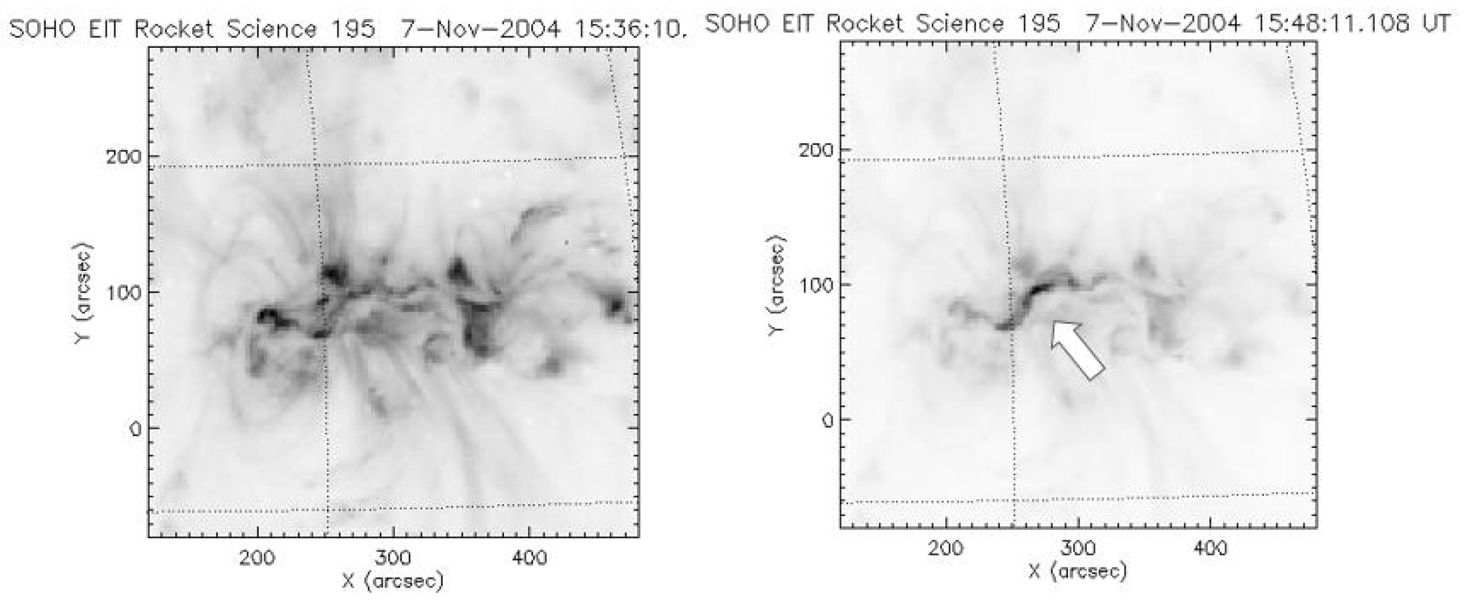
Figure 32.
(a) The solar surface observed by the RHESSI hard X-ray telescope during 16:06 -16:10 UT. The brightest point was observed at the solar coordinate (282,101), that coincides with the point indicated by the white arrow in the Figure 31(right side). The energy band of hard X-ray was 25-50 keV, while Figure 31 presents the solar surface observed by the SOHO 195 nm telescope. (b) The RHESSI image taken between 16:25-16:29 UT. The brightest point shifed toward (282, 101). The energy band of this image is in the energy range of 100-300 keV.
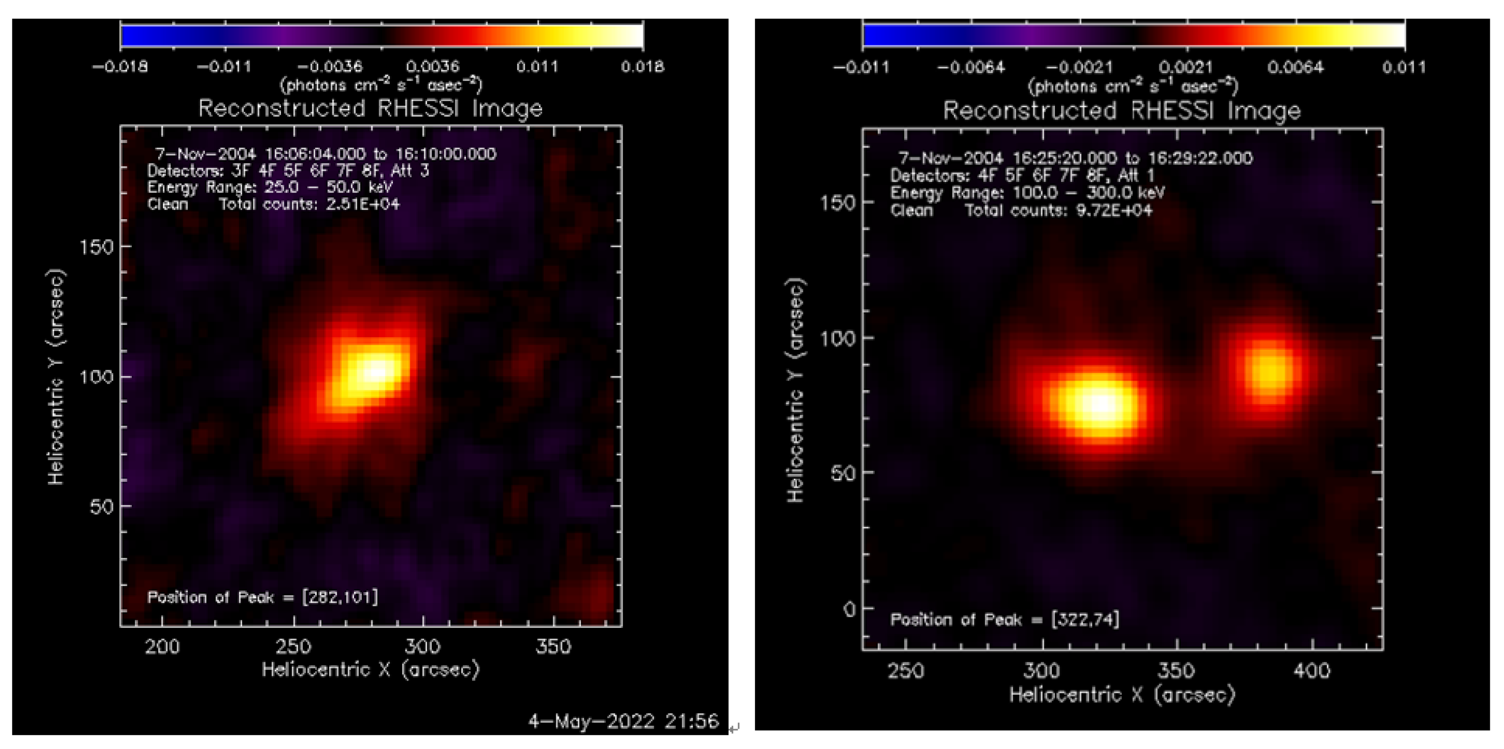
Figure 33.
The energy spectrum detected by the KONUS satellite in the energy range between 200 keV and 10 MeV. It would be interesting to know some signals around 2.223 MeV, 4.438 MeV and 6.129 MeV. The 2.223 MeV line gamma-rays are produced by the annihilation process of neutron forming deuterium, while 4.438 MeV and 6.129 MeV line gamma-rays are produced by the de-excitation process of carbon and oxygen nuclei. Furthermore, the minor enhancements in the region 1.2-2 MeV may be produced by the de-excitation process of Fe, Mg, Ne and Si nuclei.
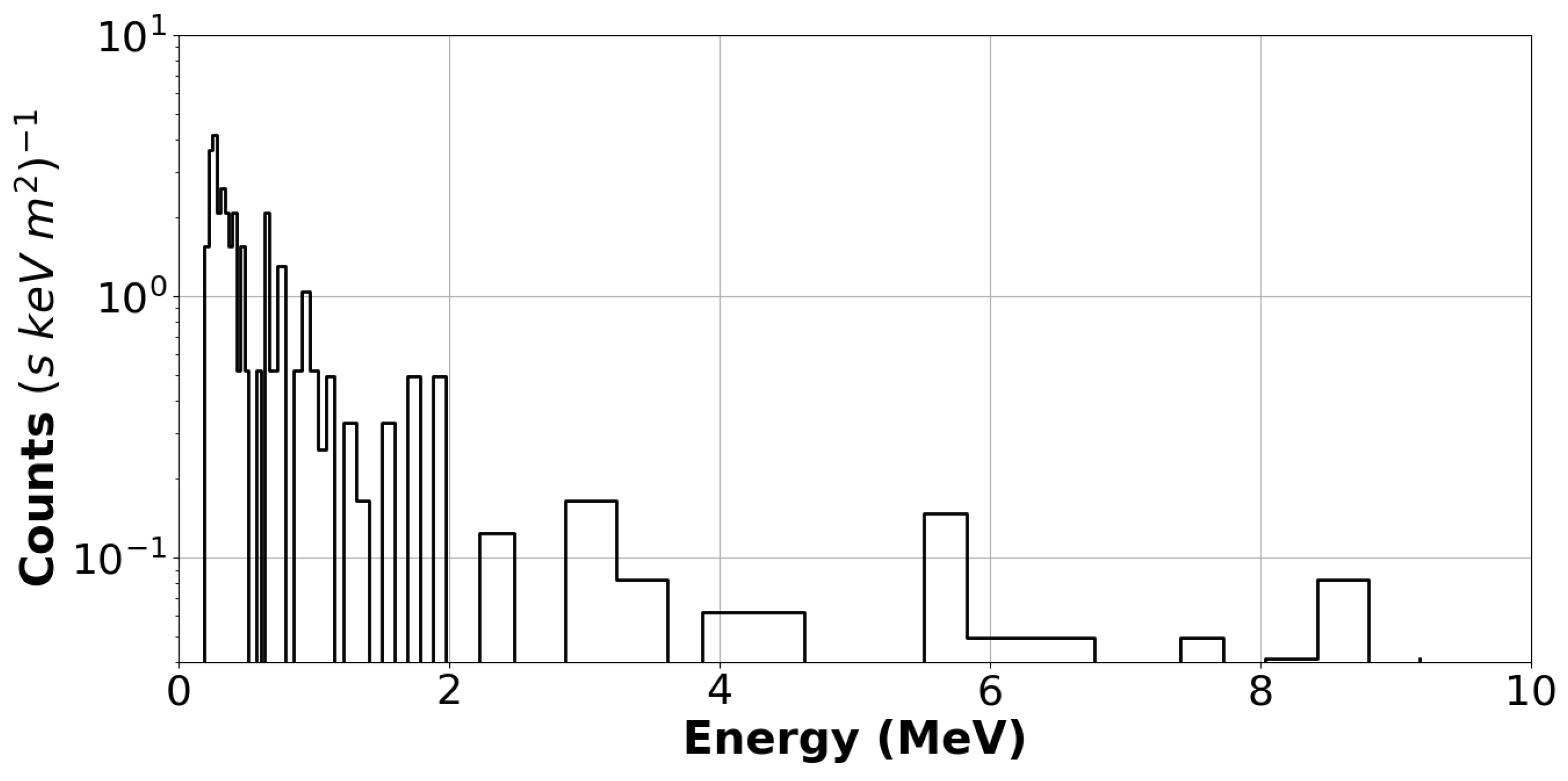

Table 1.
Type of particles recorded in each detector.
| Received particle | types Detectors | Mountain Detectors |
|---|---|---|
| Solar neutrons (n) | GOES 10, 11 | Mt. Chacaltaya |
| Solar neutron decay protons (p) | Oulu, GOES 12 | Mt. Sierra Negra |
Disclaimer/Publisher’s Note: The statements, opinions and data contained in all publications are solely those of the individual author(s) and contributor(s) and not of MDPI and/or the editor(s). MDPI and/or the editor(s) disclaim responsibility for any injury to people or property resulting from any ideas, methods, instructions or products referred to in the content. |
© 2023 by the authors. Licensee MDPI, Basel, Switzerland. This article is an open access article distributed under the terms and conditions of the Creative Commons Attribution (CC BY) license (http://creativecommons.org/licenses/by/4.0/).
Copyright: This open access article is published under a Creative Commons CC BY 4.0 license, which permit the free download, distribution, and reuse, provided that the author and preprint are cited in any reuse.


