
Submitted:
07 November 2023
Posted:
07 November 2023
You are already at the latest version
Abstract
Deep learning is based on matrix computing with a large amount of hidden parameters that is not visible outside the computing module. Deep learning is a non-linear system and a linear approach is not possible. It is natural for people to visualize the algorithm and to follow some hidden parameters. In this paper, we propose a simple graphical programming of a nonlinear system based on drawing the simplest unit, such as a single neuron model. A more complex scheme of a classical neural network is obtained by commands copy-move-place of one neuron. The number of neurons and layers can be chosen arbitrarily. Once the scheme is complete, the implementation code is evaluated with symbolic parameters and nonlinear activation functions. This cannot be done manually. With the symbolic expression of outputs in terms of inputs and symbolic parameters, including symbolic activation pure functions, some other properties can be derived in closed form. This unique original approach can help scientists and developers and design numerical algorithms for machine learning and to understand how deep learning algorithms work.
Keywords:
machine learning
; visual programming language
; closed-form expression
; theoretical justification
; feature extraction
; complexity
; optimization and validation
1. Introduction
Machine learning, as subfield of Artificial Intelligence (AI), refers to computers learning to do things on their own [1]. Machine learning (ML) is the core of AI which solves the problems of classification, clustering, and forecasting complex algorithms and methods, in order to overcome the limitations and achieve expansion of AI and ML applications [2]. There are many applications in several fields of basic science and engineering focused on some important and challenging topics, such as nonlinear problems, numerical methods, analytical methods, error analysis and mathematical models [3]. A review of a variety of experiments on extracting structure from machine-learning data is presented in [4]. Some algorithms do not need a huge set of training data and can be implemented only by applying standard templates and thus provide the high response speed [5]. Some applications with nonlinear process demonstrate the different neural network-based models [6]. Some heuristic procedures can reduce computational complexity with respect to optimal multiple sequence alignment and thus outperform humans in the post-processing of recognition hypotheses [7]. Adaptive network enhancement method for the best least squares approximation using two-layer Rectified-Linear-Unit (ReLU) neural networks is introduce in [8]. Trends for mathematical explanations of the theoretical aspects of Artificial Neural Networks (ANN), with a special attention to activation functions, can be used to absorb the defining features of each design scenario [9]. Some other researchers have developed cost estimation techniques, which are based on statistical and computational techniques [10]. Learning representations of graphs have become a popular learning model for prediction tasks for a practice [11]. Graph Neural Networks (GNNs), neural network architectures targeted to. Symbolic regression, as the task of predicting the mathematical expression of a function from the observation of its values, is a difficult task. Neural networks have recently been tasked to predict the correct skeleton in a single try, but still remain much less powerful [12].
The biggest disadvantage of machine learning is that most of them cannot be explained. Up to now, AI solved problems that are intellectually difficult for humans but relatively straightforward for computers problems. As explained in the previous paragraph, success is possible if we are using a list of formal mathematical rules. The challenge to AI is to solve the tasks that are easy for humans to perform, but formally hard to describe in spite that we can solve intuitively. The hierarchy enables the computer to learn complicated concepts by building them out of simpler ones. The graph is deep when it has many layers. For this reason, we call this approach to AI deep learning [13]. The difficulties facts by systems relying on hard-coded know knowledge suggest that AI systems need the ability to acquire their own knowledge, by extracting patterns from raw data [13]. This capability is known as machine learning. We can use mathematical function mapping some set of input values to output values. The function is formed by composing many simpler functions. The powerful root mean square error accuracy comparison of gradient boosting machines (a popular machine learning regression tree algorithm) we can use to avoid the multicollinearity of multivariate input variables with the simulated normal distribution data [14]. For solving decision-making problems in both computer science and engineering, we can use Optimization Machine Learning Toolkit as an open-source software package incorporating neural network [15]. Software tools can simplify training neural networks, using machine learning, from simpler into larger optimization problems.
Recent advances in machine learning have led to increased interest in solving visual computing problems using methods that employ coordinate-based neural networks. These methods we call neural fields. [16]. Machine learning tools are part of Wolfram Language that performs classification, regression, dimensionality reduction and neural network processing. The book [1] takes a "show, don't tell" approach and we use the same examples to show how to use the Wolfram Language [17]. Using a visual programming language (the SchematicSolver application package [18], requires software Mathematica 9 [17]) we can develop own algorithms and understand the architecture of complex networks. Mathematical education at the end of high school should be sufficient to understand mathematical content [1]. A visual programming or GUI (Graphical User Interface) can provide fast interactive design, symbolic analysis, accurate simulation, exact verification, and reports [19]. It helps to skip the gap between theory and practice in continuous-time systems. The mathematical representation of the system can be obtained automatically from the schematic description, and automated symbolic manipulations are possible.
Although accurate, AI models often are “black boxes” which we are not able to understand [20]. Transfer learning is a powerful approach that leverages knowledge from one domain to enhance learning in another domain; it provides practical insights for researchers and practitioners interested in applying transfer learning techniques [21]. The pervasive success in predictive performance comes alongside a severe weakness, the lack of explainability of their decisions, especially relevant in human-centric [22]. From black-box to explainable AI in healthcare: existing tools and case studies [23].
Convolutional Neural Networks (CNNs) constitute a widely used deep learning approach that has frequently been applied to the problem of brain tumor diagnosis. Such techniques still face some critical challenges in moving towards clinic application [24]. The smart visualization of medical images (SVMI) model is based on multi-detector computed tomography (MDCT) data sets that can provide a clearer view of changes in the brain, such as tumors (expansive changes), bleeding, and ischemia on native imaging. The new method provides a more precise representation of the brain image by hiding pixels that are not carrying information and rescaling and coloring the range of pixels essential for detecting and visualizing the disease [25].
The main trends with which machine learning techniques have been applied to robotic manipulation are presented in [26]. Resources in the robotics field are limited for a common user to access and demand deep knowledge of robot programming paradigm. It is presented how to program control algorithms and to control complex robotic systems by using widespread and inexpensive devices such as smartphones and tablets, Android operating system, for simulation and remote control of robotic manipulators [27]. The review paper on deep learning-assisted smart process planning, robotic wireless sensor networks and geospatial big data management algorithms in the internet of manufacturing things configures on deep learning-assisted smart process [28]. The paper [29] presents a system for programming and simulation of the human centrifuge motion with integrated 3D motion simulator. The simulator can be used for verification of newly defined motion commands and testing the new algorithms for the human centrifuge motion.
Analog designs that implement various machine learning algorithms can be useful in low-power deep network accelerators suitable for edge or tiny machine learning applications [30]. Analog circuit design requires large amounts of human knowledge; a special case of circuit design is the synthesis of robust and failure-resilient electronics [31]. An example of dissipation minimization of two-stage amplifier using deep learning is presented in [32] (deep learning is a subset of machine learning). The deep learning module controls the operating mode of the amplifier which is a function of the average input signal. The application of VLSI (Very Large Scale Integrated) circuit in AI is described in [33]. VLSI is the inter-disciplinary science of utilizing advance semiconductor technology to create various functions of computer system such as the close link of microelectronics and AI. By combining VLSI technology, a very powerful computer architecture confinement is possible.
The purpose of this paper is an attempt to explain machine learning models using algorithm visualization. The main goal of the work is the final results as expressions in a closed form where the developer can change and monitor hidden parameters.
2. Materials
Deep learning can involve learning using an artificial neural network. Humans have about one hundred billion biological neurons in their brain and about ten thousand times more connections. A neuron has its inputs , , ..., , via input branches. The neuron then calculates an electrical output , that is sent to other neurons through tiny intercellular connections.
Artificial neural networks use the same basic principles that are much simpler than their biological neurons. For given input values , , ..., , the artificial neuron has only one output , whose value is calculated by the formula:
The parameters, , , ..., , change during neuron operation and are interpreted as strengths of the connection between neurons. They are called weights or weight parameters. The parameter is called the bias and is interpreted as the threshold at which the neuron is activated. The nonlinear function is called the activation function or the transfer function.
An illustration of the calculation of an artificial neuron (which gives the same output expression as it should theoretically be) is given in the Figure 1 (drawn with SchematicSolver ver2.3 [18] that is written using Wolfram language, Mathematica ver. 13 [17]):
The first part is a linear combination of the inputs, and then the nonlinearity is applied. Nonlinearity allows neuron to model nonlinear system. Biological neurons are either activated or not. Therefore, it is tempting to use some kind of activation function. Artificial neurons used logistic sigmoid function, hyperbolic tangent function or Ramp function (rectified linear unit, ReLU) that works pretty well in deep neural networks [1], see Figure 2:
3. Methods
In Figure 3 on the left, the architecture of the artificial neuron is drawn, where the input signals , , ..., , are separated from the parameters that are modified during the operation of the neuron. The same figure on the right shows a block diagram of a neuron that depends exclusively on input signals, and the parameters , , ..., , that are listed as inputs through which the output is calculated. It is important to note that multipliers with constant values are not used as in linear systems, because the parameters , , ..., and , are not constants. They are modified during the operation of the neuron.
By connecting a large number of artificial neurons, networks can be made. Circles represent numerical values called activations. It is understood to be a linear combination of its inputs, plus some bias term, and the result is passed through the nonlinearity. The simplest network has two input values and one output value. The graph is directed and acyclic, so the output can be calculated simply by following the arrows.
This network is a parametric model. There is one weight parameter per input and one bias parameter per neuron. We could train this network in the same way as any other parametric model: by minimizing a cost function calculated from some training data. The architecture does not change; only the numerical values of the parameters (weights and biases) are changed. Familiar architecture is used; neurons are grouped in layers and each neuron in one layer sends its output to each neuron in the next layer. These fully connected layers are also called linear layers.
Let the network consist of several layers, and let there be four neurons in each layer. Four input signals come to the first layer. The output of each neuron generates only one output, and since there are 4 neurons, 4 output signals are generated. The output signals of the first layer become the input signals for the second layer, which also has 4 neurons and generates 4 output signals. The output signals of the second layer are the input signals of the third layer, which also has 4 neurons with 4 output signals. The output signals of the third layer are the outputs of the neural network. The first and second layers are called hidden layers because the outputs of the neurons are not seen outside the network.
The number of input signals to the first layer must not be greater than 4, and to ensure that some of the 4 network inputs do not affect the network outputs, the weight parameters are set to 0 from the network inputs in the first layer to the adders.
Assume that there are only two numeric values as inputs and that the first layer generates four numeric values as the output of the first hidden layer. Now the input of the second hidden layer has 4 numerical values as inputs, and it generates 4 output values which are the values of the third layer neurons. These four inputs generate 4 output numerical values that become the outputs of the neural network, and therefore the third layer is not a hidden layer because the results are visible. The activation function generates one of the 4 classes to which the processing result belongs, and the activation function is unambiguously mapped to the output, that is, the one that has all positive results (all probabilities must be positive) and the sum of all probabilities (outputs) is used as a nonlinear function of the last layer) must be 1 (sum of probabilities of all classes must be 1). Such a network is used to train a classifier that has four possible classes, and the output values would then be the class probabilities. For a regression task, you would have only one output (predicted value) and that is the class that is most likely.
In this example, two hidden layers are included, but there could be many more. A network with two or more hidden layers is called a deep network, hence the name "deep learning". This name emphasizes the importance of using models that can perform several computational steps.
3.1. Matrix representation
As an illustration of how a neural network works, we will analyze a network that has 4 neurons in three layers as a minimal deep learning network. Usually, a mathematical approach is used through matrices, which are easily implemented in numerical programs. The first input layer contains 4 weight coefficients for each neuron, so a total of 2×4=8 parameters for the weights of the first layer to calculate the output values of the first hidden layer. One bias parameter per output is added. Visually, the weight parameters are represented as a 4×4=16 matrix (for four neurons, each with 4 weights), and a 1×4=4 matrix (for four neurons, each with one 1 bias parameter). For input values, we will use a 1×4=4 matrix with numerous values that can be input signals to the network or output signals of the previous layer. The matrix representation is as follows according [x1]:
where:
3.2. Matrix computation
The activation function is chosen to be the hyperbolic tangent. For only two inputs, numerous values were arbitrarily chosen, while the remaining two inputs were set to 0. All parameters were obtained by a random number generator (RandomReal) in the Wolfram language. In order to obtain always the same numerical value, the function SeedRandom[123] is used. Now the number values for the first layer are rounded to 3 decimal places, according to [x1]:
To make sure that the third and fourth inputs do not affect the result, some weight parameters are set to 0. This is therefore a network with only two inputs.
The output values of the first hidden layer are represented as a matrix Y. These values become the inputs for the next layer, so the following values are obtained for the second hidden layer:
The output values of the second hidden layer are shown as the matrix Y. These values become the inputs to the output layer, so the following values are obtained for the third layer:
The output values of the last layer do not use the hyperbolic tangent for the activation function, but the so-called softmax function that calculates the probability of the occurrence of an output:
The fourth outcome has a probability of 0.600, i.e. 60.0%, the first and third outcomes have a probability of 0.184 (18.4%) and the first outcome has a probability of 0.031 (3.1%). All probabilities must be positive, and the sum of probabilities must be 1 (the first decimal place may have a difference due to rounding).
A classifier that has parameters, as in this example, shows that the most likely result is class 4. The weight parameters , , ..., and the bias parameter change during the operation of the neuron. In total, in the analyzed network with two hidden layers and one output layer of 4 neurons, there are 3×4×4=48 weight parameters and 3×1×4=12 bias parameters, i.e. in total the analyzed network has 48+12=60 parameters which are changed during neural network processing.
4. Results
In computing it is natural to use a matrix data structure. It is more natural for people to see an architectural sketch.
4.1. Symbolic computation
Firstly we will draw the architecture of one layer consisting of 4 neurons using SchematicSolver [18] as shown in Figure 4.
Inputs and outputs are drawn separately for a neural network with one or more layers, Figure 4(a) and Figure 4(c). Using one layer, Figure 4(b), the neural network is obtained by joining the input, output and one layer shown in Figure 4(d).
To draw a neural network with three layers, an already drawn layer, image in Figure 4(b) is used, which is copied the necessary three times to the right with a raster of 13 (how wide the base layer is) and the output layer is shifted to the right by 3×13=39. Symbolic parameter names and activation functions are changed with each copy. The complete scheme is obtained by connecting the inputs, outputs and all layers and is shown in Figure 5.
It is important to notice that the activation function of the final layer is different, g such that the output values are equal to the class probabilities.
4.2. Symbolic solving
By clicking on the button to implement the schematic from the image drawn in SchematicSolver, the implementation code is obtained, a small part of which is in Figure 6(a).
Symbolically derived expressions for 4 classes use almost 316KB. Such a performance in closed form is not possible to derive manually. Visually, it can be seen that the graph with all levels is very complex. The symbolically derived expression can be used for further analysis, which is not possible for a purely numerical approach. By changing the symbolic values with the numerical parameters from the matrix approach, the same probabilities are obtained, a 60.0% probability that the classification number is 4 as with matrix computing.
4.3. Symbolic analysis
In the same way, a neural network with 4 layers is obtained, of which 3 are hidden layers. With the same values for the parameters as with 2 hidden layers, but with the addition of randomly generated values for the newly added layer, a probability of 63.8% is obtained for class 2. The complexity of the closed-form final expressions in the symbolic notation is shown in Figure 7. This derivation exceeds manual execution.
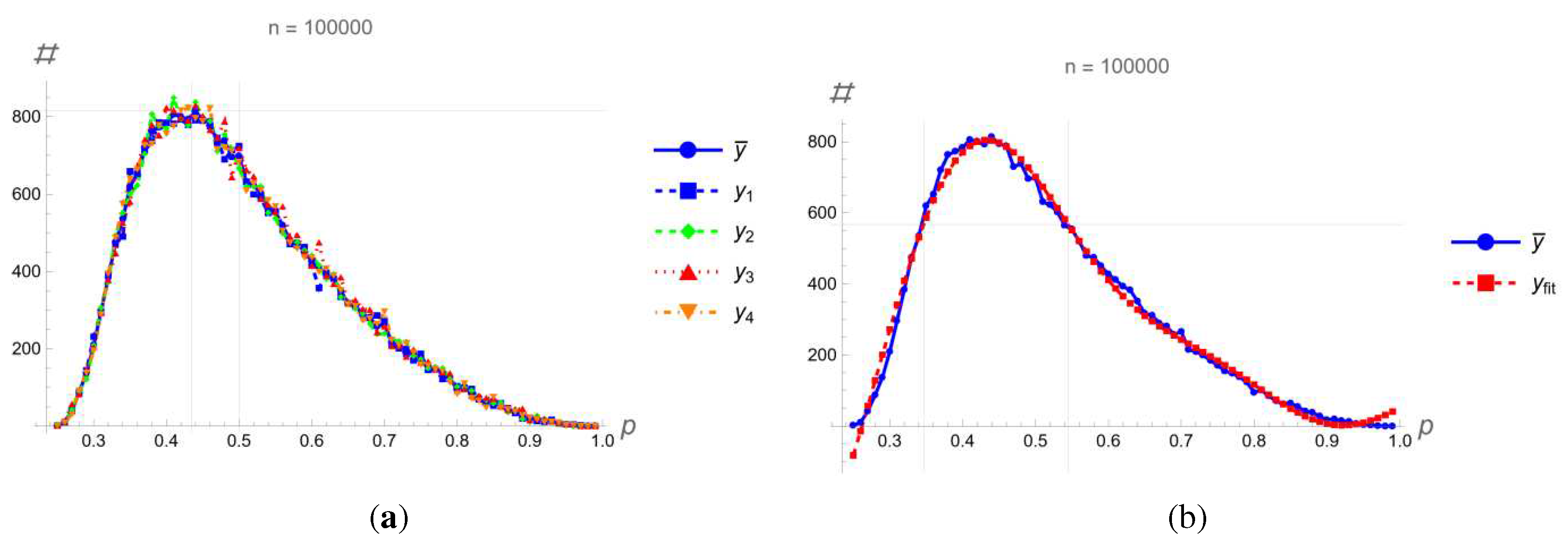
The symbolically obtained response of the neural network enables further analysis without the use of schematics. With 100,000 randomly generated parameters, probabilities for all outputs were determined as shown in Figure 8. .
For the mean value, an expression was derived in closed form:
The most likely probability was calculated when the maximum number of classes was detected, which is for a probability of 43.3%, when 800 cases were detected. For 0.7071 in relation to the maximum, the range in which there is the largest number of certain classes was calculated, which is for the range between 34.7% to 54.4% probability. Half of all classes were detected for this range. It is important to note that there cannot be a probability of less than 25% when a class is detected, because at least one other class would have a probability of more than 25%. Each class was detected approximately 25,000 times, and no case was detected where all classes were equally likely. In all cases, the same input signal values were used:
For all classes and all probabilities, all parameter values are equally likely, that is, there is no parameter value where the probability of detecting one of the 4 classes would be more pronounced.
5. Discussion
The disadvantage of using machine learning as black box is overcome by designing non-linear system using visual programming. During test or validation process, system parameters can be viewed for verification purposes. The final results as expressions in a closed form can be derived and optimized according the required task. The future development is looking for fully automated design based on required number of neurons in a layer as well as the number of layers. There is no similar approach as the best knowledge of the authors.
Supplementary Materials
All programs are available from the corresponding author as well as from the journal repository.
Author Contributions
Conceptualization, M.L.B. and N.Z.; methodology, M.L.B. and V.M.; software, M.L.B. and N.D.; validation, M.L.B., V.M. and N.D.; formal analysis, M.L.B. and I.F.; investigation, M.L.B. and I.F.; resources, M.L.B. and N.D.; data curation, M.L.B. and N.Z.; writing—original draft preparation, M.L.B. and N.D.; writing—review and editing, M.L.B. and N.Z.; visualization, N.Z. and I.F.; supervision, M.L.B., V.M. and I.F.; project administration, V.M.; funding acquisition, I.F., V.M., N.Z. and N.D. All authors have read and agreed to the published version of the manuscript.
Funding
This research received no external funding.
Institutional Review Board Statement
Not applicable.
Informed Consent Statement
Not applicable.
Data Availability Statement
All programs are available from the corresponding author.
Conflicts of Interest
The authors declare no conflict of interest.
Appendix A
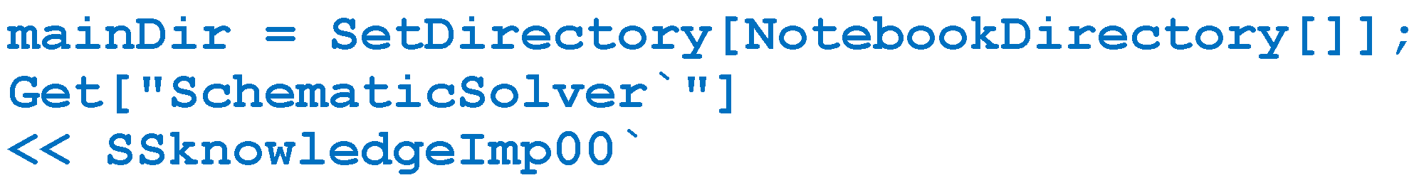
We use the Wolfram language for programming. The code is in the form of readable text with the extension .nb. The first step is to set the working directory and import the knowledge as a package or text file with the extension .m:
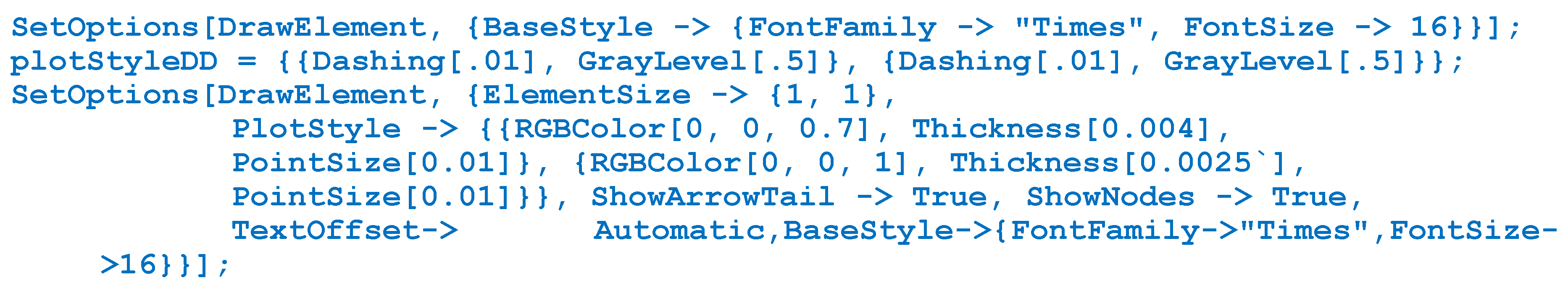
The next few lines of the program tell how the scheme is visible in the images:
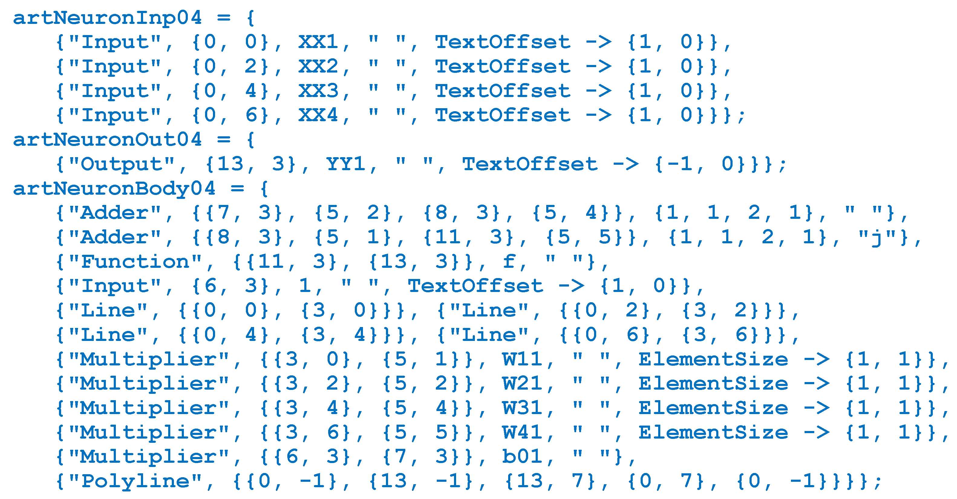
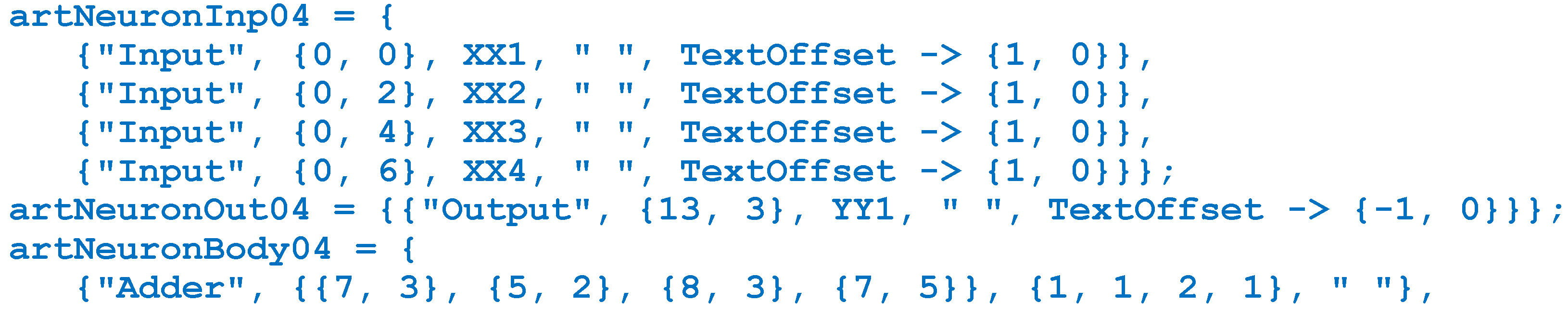
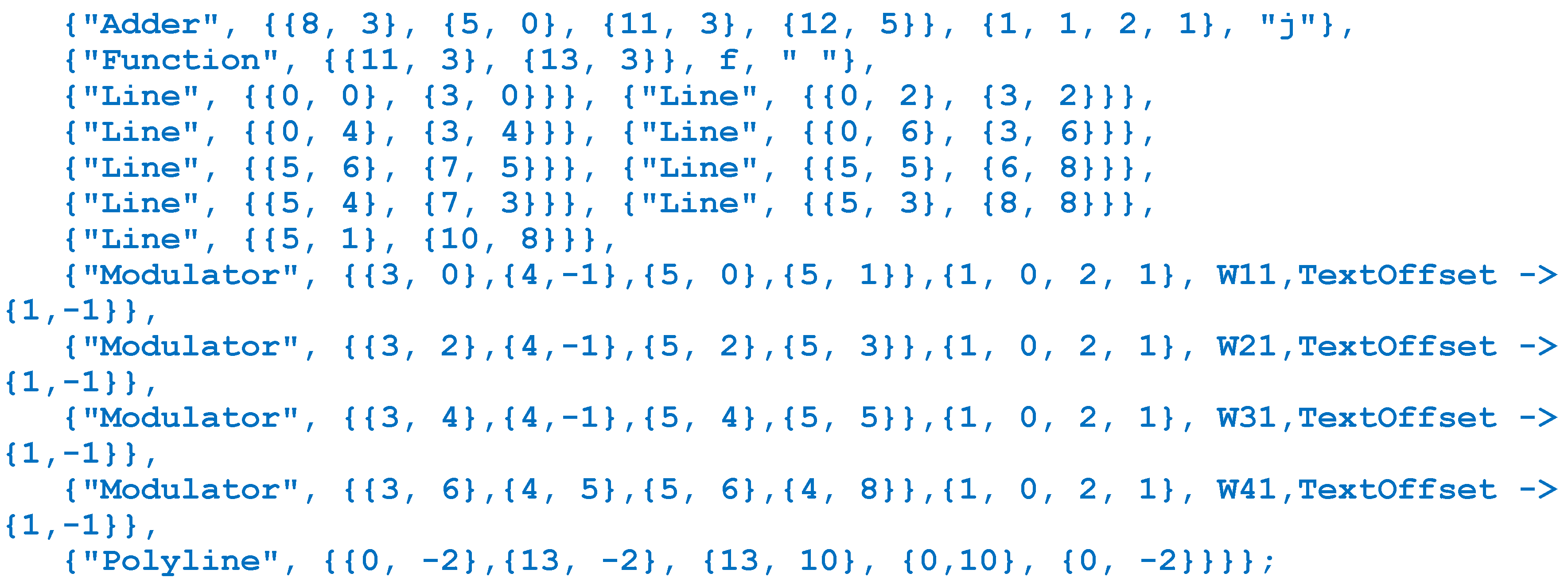
Input, output, and single-layer schemes are defined as separate lists:
Replacement rules are used for drawings (represented in bitmap format):
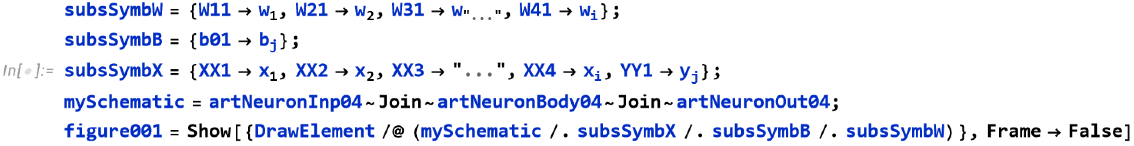
Figure 1 was created with the previous code.
Appendix B
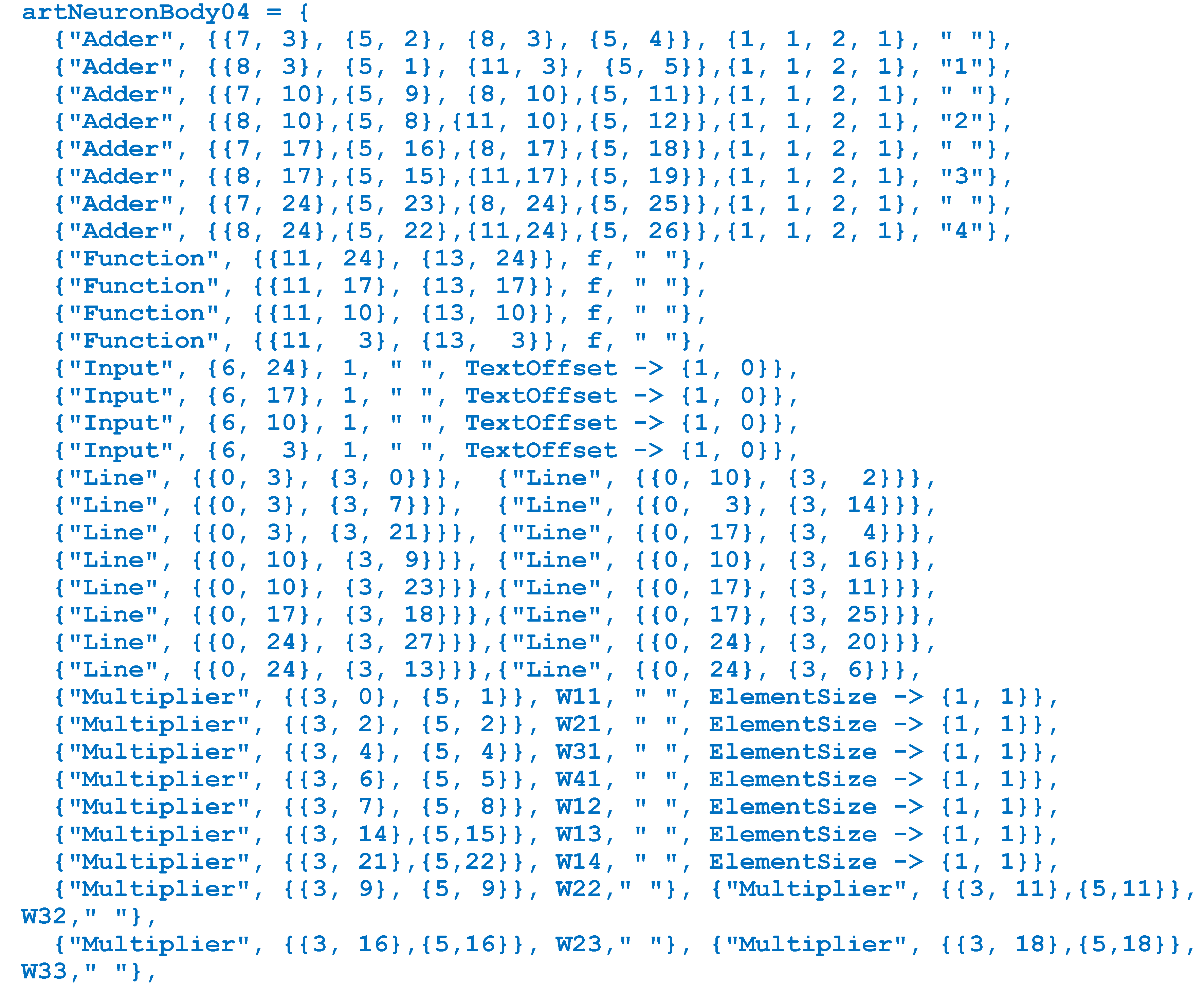
Figure 3(a) was created with the next code:
Notice that we are using Modulator instead of Multiplier. The Delay elements are presented in bitmap format:
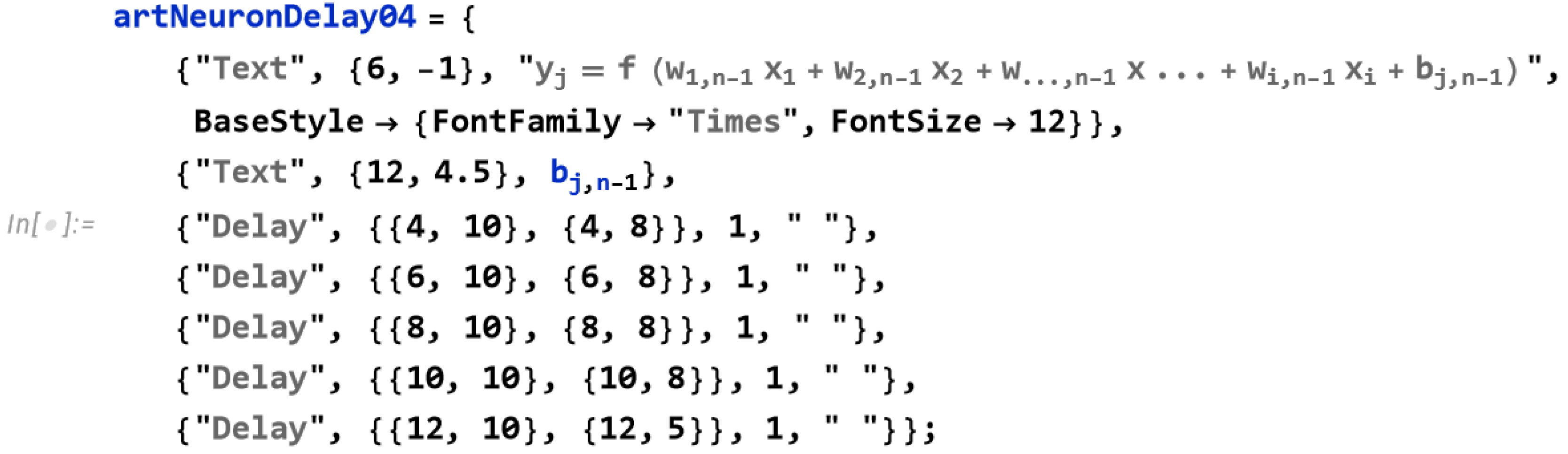
Figure 3(b) was created with the similar code.
Appendix C
Figure 4(b) was created with the next code:
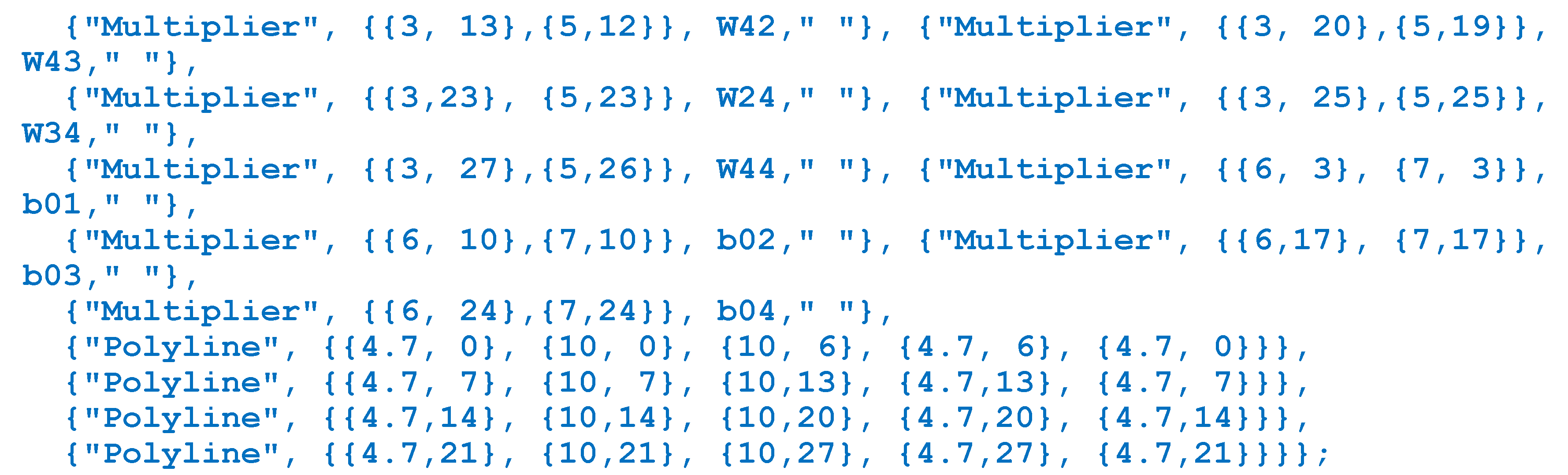
The initial layer can be translated and copied 3 times using Do command:
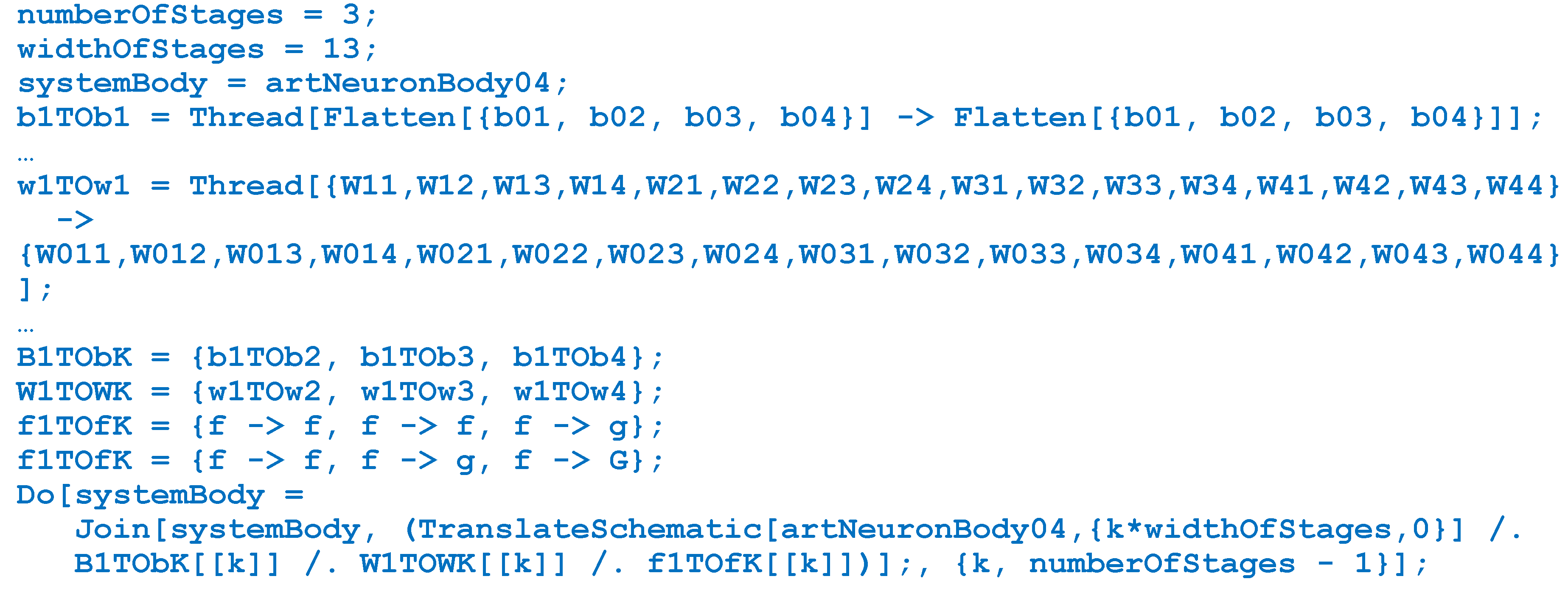
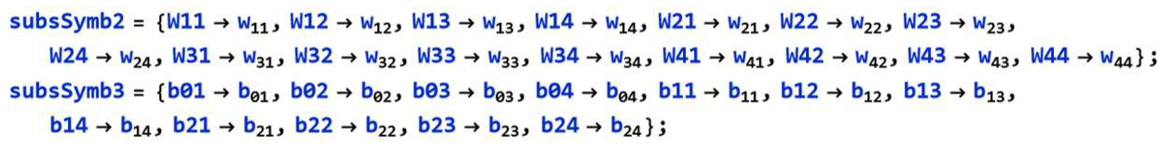
Each symbol can be presented in different mathematical notation.
For the previous code we are using bitmap presentation.
Appendix D
The closed-form outputs are derived using the next code:
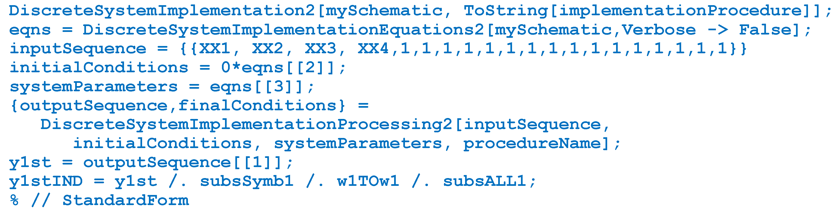
Figure 7(b) is obtained using ExpressionGraph command.
References
- Bernard, E. Introduction to Machine Learning; Wolfram Media: Champaign, IL USA, 2022; pp. 1–424. [Google Scholar]
- Mukhamediev, R.; Popova, Y.; Kuchin, Y.; Zaitseva, E.; et al. Review of artificial intelligence and machine learning technologies: classification, restrictions, opportunities and challenges. Mathematics 2022, 10(15), #2552, 1-25.
- Juraev, D.; Noeiaghdam, S. Modern problems of mathematical physics and their applications. Axioms 2022, 11(2), 1–6. [Google Scholar] [CrossRef]
- He, Y. H. Machine-learning mathematical structures. IntJDataS.Math.S 2023, 1(01), 23–47. [Google Scholar] [CrossRef]
- Rajebi, S.; Pedrammehr, S.; Mohajerpoor, R. A license plate recognition system with robustness against adverse environmental conditions using Hopfield’s neural network. Axioms 2023, 12(5), 1–12. [Google Scholar] [CrossRef]
- Ren, Y.M.; Alhajeri, M.S.; Luo, J.; Chen, S.; Abdullah, F.; Wu, Z.; Christofides, P. D. A tutorial review of neural network modeling approaches for model predictive control. Comp.Chem.Eng. 2022, 165, 1–71. [Google Scholar] [CrossRef]
- Gnjatović, M.; Maček, N.; Saračević, M.; Adamović, S.; Joksimović, D.; Karabašević, D. Cognitively economical heuristic for multiple sequence alignment under uncertainties. Axioms 2022, 12(1), 1–15. [Google Scholar] [CrossRef]
- Liu, M.; Cai, Z. Adaptive two-layer ReLU neural network: II. Ritz approximation to elliptic PDEs. Comp.Math.App. 2023, 113, 103–116. [Google Scholar] [CrossRef]
- Cabello, J.G. Mathematical neural networks. Axioms 2022, 11(2), 1–18. [Google Scholar] [CrossRef]
- Refonaa, J.; Huy, D.T.N.; Trung, N.D.; Van Thuc, H.; Raj, R.; Haq, M.A.; Kumar, A. Probabilistic methods and neural networks in structural engineering. Int.J.Adv.Manuf.Techn. 2022, 125(3-4), 1-9.
- Jegelka, S. Theory of graph neural networks: representation and learning. In Proceedings of the Int. Congress of Mathematicians, (virtual event, originally planned Saint Petersburg, Russia), Helsinki, Finland, 6-14 July 2022.
- Kamienny, P.A.; d'Ascoli, S.; Lample, G.; Charton, F. End-to-end symbolic regression with transformers. Adv.Neural Inf.Proc.Syst. 2022, 35, 10269–10281. [Google Scholar]
- Goodfellow, I.; Bengio, Y.; Courville, A. Deep Learning; The MIT Press: Cambridge, MA USA, 2022; pp. 1–800. [Google Scholar]
- Kim, J.M.; Kim, J.; Ha, I.D. Application of deep learning and neural network to speeding ticket and insurance claim count data. Axioms 2022, 11(6), 1–185. [Google Scholar] [CrossRef]
- Ceccon, F.; Jalving, J.; Haddad, J.; Thebelt, A.; et al. OMLT: optimization & machine learning toolkit. J.Mach.Learn.Research. 2022, 23(1), 15829–15836. [Google Scholar]
- Xie, Y.; Takikawa, T.; Saito, S.; Litany, O.; et al. Neural fields in visual computing and beyond. STAR. 2022, 41(2), 1–36.
- Wolfram, S. An Elementary Introduction to the Wolfram Language, 3rd ed.; Wolfram Media: Champaign, IL USA, 2023; pp. 1–376. [Google Scholar]
- SchematicSolver. Available online: https://www.wolfram.com/products/applications/schematicsolver (accessed on 17 10 2023).
- Lutovac-Banduka, M.; Milosevic, D.; Cen, Y.; Kar, A.; Mladenovic, V. Graphical user interface for design, analysis, validation, and reporting of continuous-time systems using Wolfram language. JCSC 2023, 32. # 2350244, 1-14. [Google Scholar] [CrossRef]
- Setzu, M.; Guidotti, R.; Monreale, A.; Turini, F.; et al. GLocalX – from local to global explanations of black box AI models. Artificial Intelligence. 2021, 294(103457), 1–15. [Google Scholar] [CrossRef]
- Ghelani, D. Explainable AI: approaches to make machine learning models more transparent and understandable for humans. IJCST. 2022, 6(4), 45–53. [Google Scholar]
- Swamy, V.; Radmehr, B.; Krco, N.; Marras, M.; Käser, T. Evaluating the explainers: black-box explainable machine learning for student success prediction in MOOCs. In Proceedings of the 15th International Conference on Educational Data Mining, Durham, England, 24-27 July 2022. [Google Scholar]
- Srinivasu, P. N.; Sandhya, N.; Jhaveri, R. H.; Raut, R. From black-box to explainable AI in healthcare: existing tools and case studies. Mob.Inf.Syst. 2022, 2022, 1–20. [Google Scholar]
- Xie, Y.; Zaccagna, F.; Rundo, L.; Testa, C.; Agati, R.; et al. Convolutional neural network techniques for brain tumor classification (from 2015 to 2022): review, challenges, and future perspectives. Diagnostics. 2022, 12(8), 1–46. [Google Scholar] [CrossRef] [PubMed]
- Simović, A.; Lutovac-Banduka, M.; Lekić, S.; Kuleto, V. Smart visualization of medical images as a tool in the function of education in neuroradiology. Diagnostics 2022, 12, 3208, 1–19.
- Vuong, Q. Machine Learning for Robotic Manipulation. arXiv e-prints. 2021, arXiv-2101.00755, 1-15.
- Lutovac Banduka, M. Robotics first – a mobile environment for robotics education. Int.J.Eng.Edu. 2016, 32(2), 818–829. [Google Scholar]
- Lăzăroiu, G., Andronie, M., Iatagan, M., Geamănu, M., Ștefănescu, R., & Dijmărescu, I. Review deep learning-assisted smart process planning, robotic wireless sensor networks, and geospatial big data management algorithms in the internet of manufacturing things. IoMT. 2022, 11(5), 1-26.
- Lutovac-Banduka, M.; Kvrgić, V.; Ferenc, G.; Dimić, Z.; Vidaković, J. 3D simulator for human centrifuge motion testing and verification, In Proceedings of Mediterranean Conference on Embedded Computing, Budva, Montenegro, 15-20 June 2013.
- Liu, S.C.; Strachan, J.P.; Basu, A. Prospects for analog circuits in deep networks. In Analog Circuits for Machine Learning, Current/Voltage/Temperature Sensors, and High-speed Communication Advances in Analog Circuit Design, Harpe, P., Makinwa, K., Baschirotto, Eds.; Springer: Heidelberg, Germany, 2022; Volume 1, pp. 49–61. [Google Scholar]
- Rojec, Ž.; Fajfar, I.; Burmen, Á. Evolutionary synthesis of failure-resilient analog circuits. Mathematics 2022, 10(1), #156, 1-20.
- Lutovac-Banduka, M.; Simović, A.; Orlić, V.; Stevanović, A. Dissipation minimization of two-stage amplifier using deep learning. SJEE 2023, 20, 129–145. [Google Scholar] [CrossRef]
- Sahu, A.; Behera, S. VLSI techniques used in AI. Dogo Rangsang Res.J. 2019, 9(3), 965–967. [Google Scholar]
Figure 1.
Illustration of the computation made by an artificial neuron.
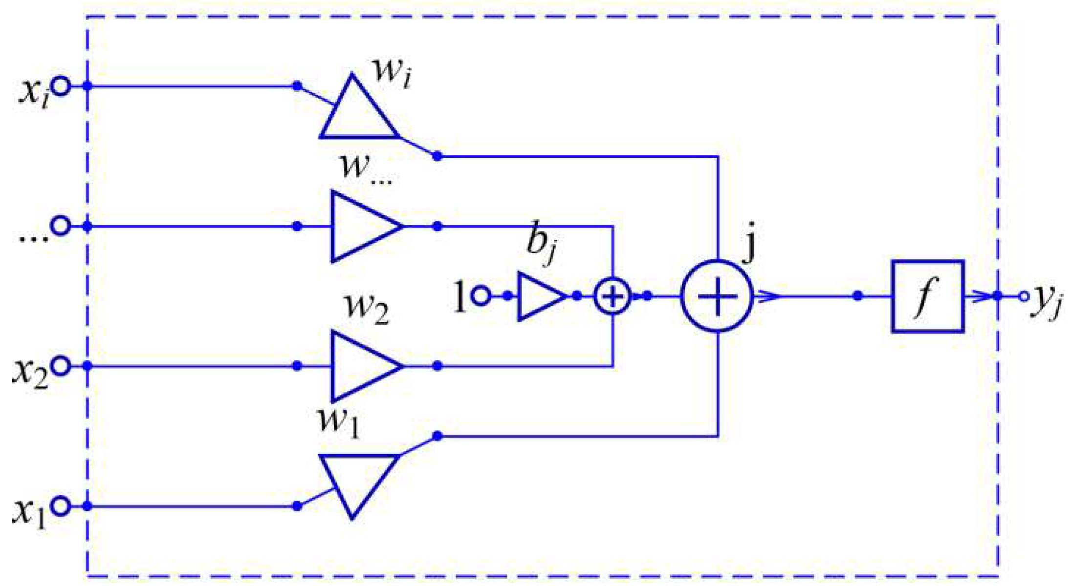
Figure 2.
Classic activation functions as rectified linear unit ReLU, logistic sigmoid σ(x), or hyperbolic tangent function tanh(x).
Figure 2.
Classic activation functions as rectified linear unit ReLU, logistic sigmoid σ(x), or hyperbolic tangent function tanh(x).
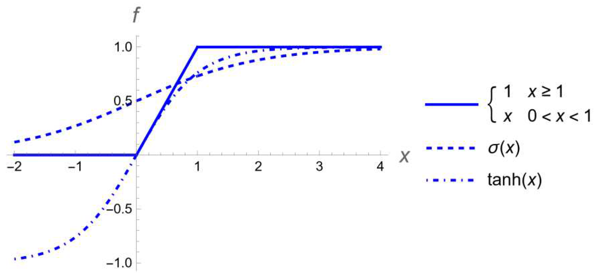
Figure 3.
Classic artificial neuron (a) with memory elements, (b) simplified.
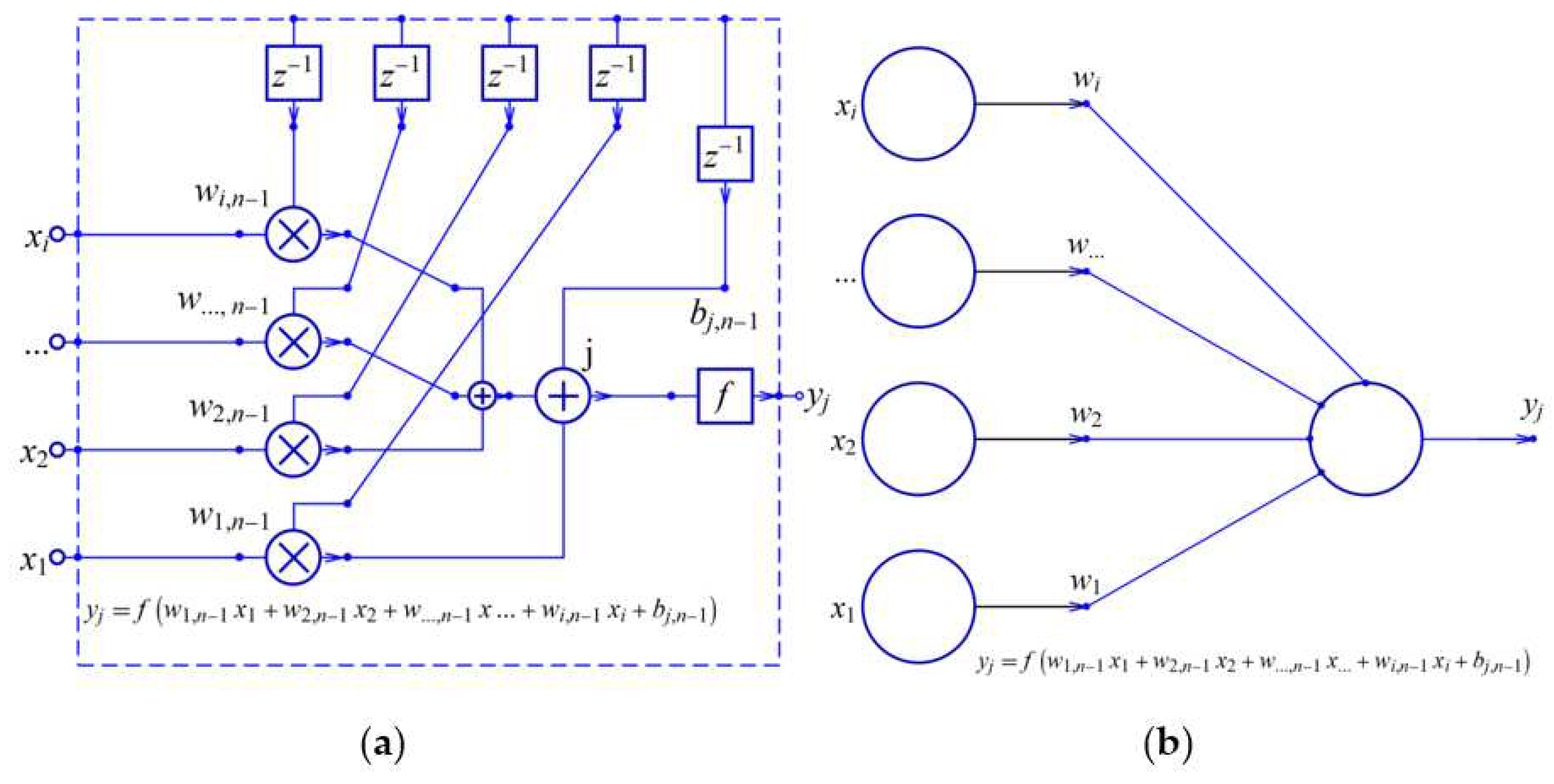
Figure 4.
Classic artificial neural network with single layer: (a) 4 inputs, (b) layer with 4 neurons, (c) 4 outputs, (d) overall schematic.
Figure 4.
Classic artificial neural network with single layer: (a) 4 inputs, (b) layer with 4 neurons, (c) 4 outputs, (d) overall schematic.
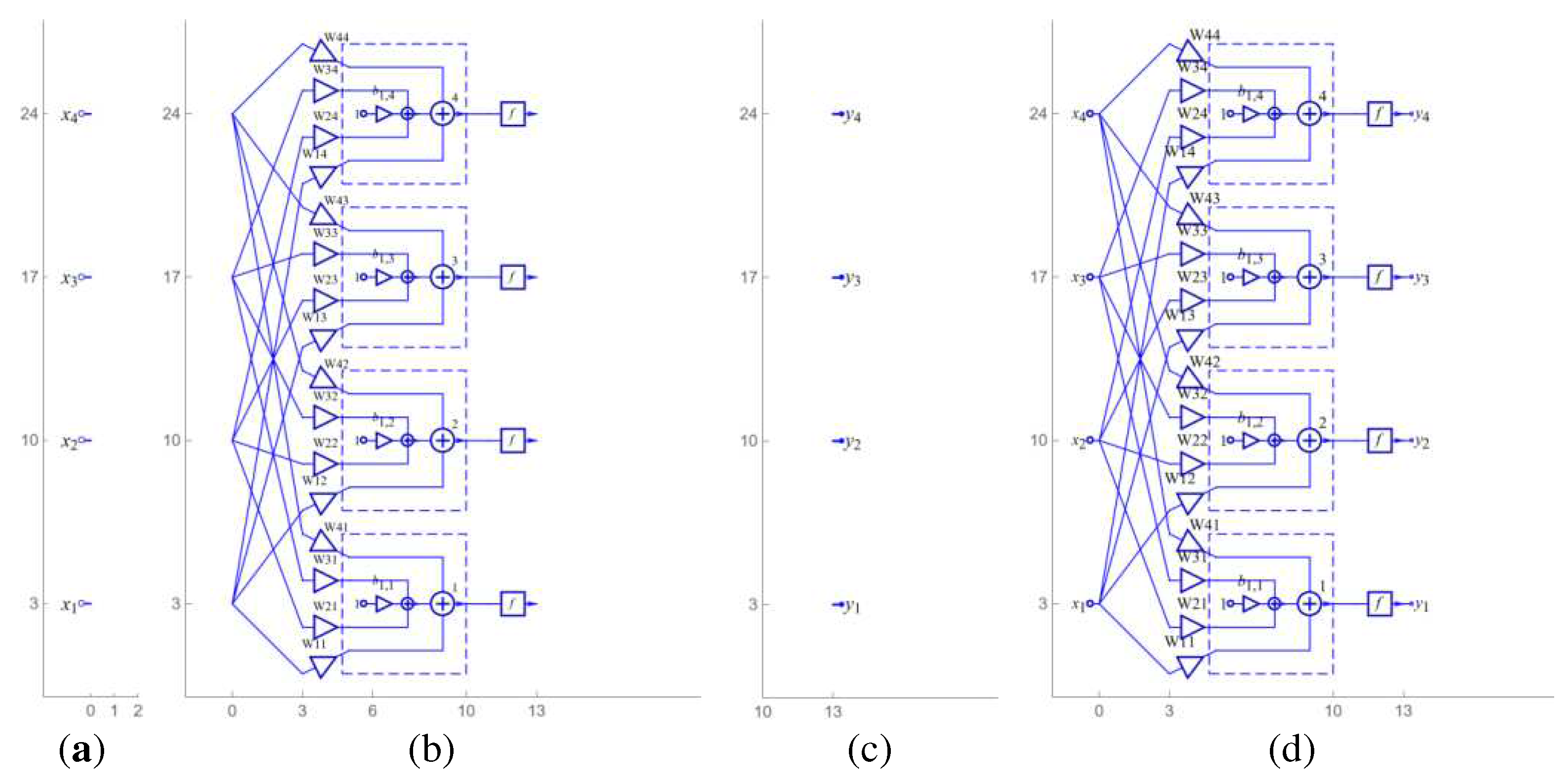
Figure 5.
Classic artificial neural network with 3 layers.
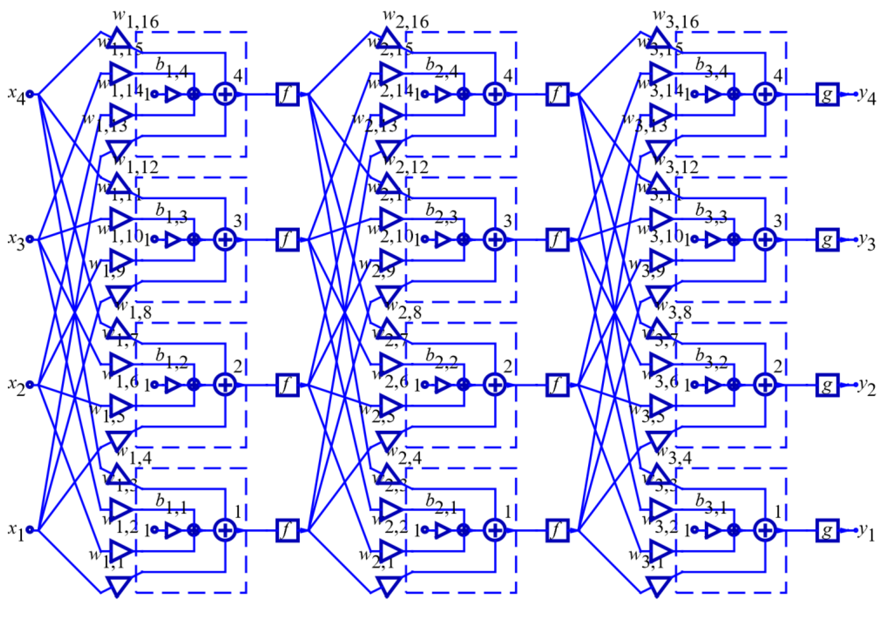
Figure 6.
Classic artificial neural network with 3 layers: (a) smaller part of symbolic response, (b) size of response, and (c) tree graph with different levels at different depths.
Figure 6.
Classic artificial neural network with 3 layers: (a) smaller part of symbolic response, (b) size of response, and (c) tree graph with different levels at different depths.
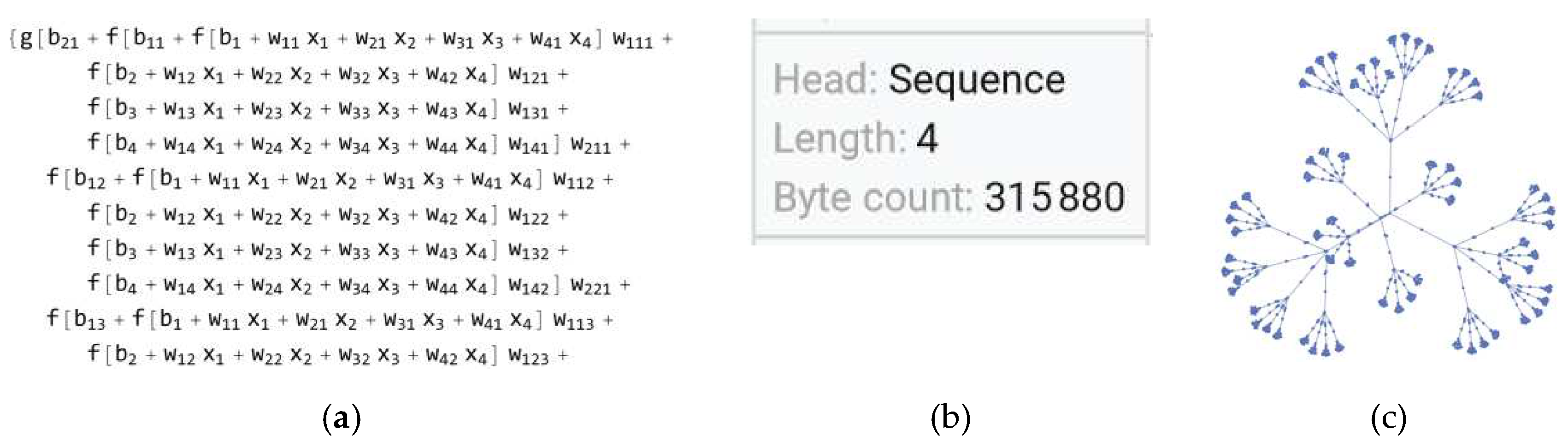
Figure 7.
Classic artificial neural network with 4 layers: (a) probabilities of four classes and (b) tree graph with different levels at different depths.
Figure 7.
Classic artificial neural network with 4 layers: (a) probabilities of four classes and (b) tree graph with different levels at different depths.
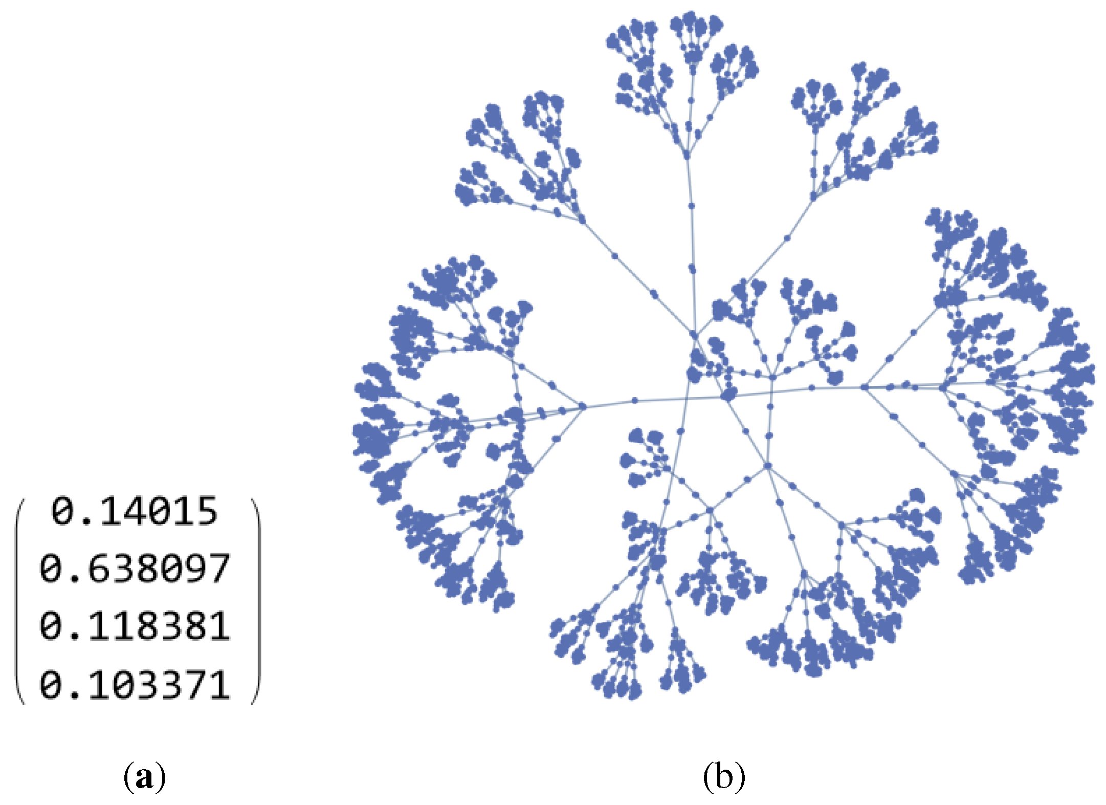
Figure 8.
(a) Class probabilities of all outputs and (b) mean value of probabilities.
Disclaimer/Publisher’s Note: The statements, opinions and data contained in all publications are solely those of the individual author(s) and contributor(s) and not of MDPI and/or the editor(s). MDPI and/or the editor(s) disclaim responsibility for any injury to people or property resulting from any ideas, methods, instructions or products referred to in the content. |
© 2023 by the authors. Licensee MDPI, Basel, Switzerland. This article is an open access article distributed under the terms and conditions of the Creative Commons Attribution (CC BY) license (http://creativecommons.org/licenses/by/4.0/).
Copyright: This open access article is published under a Creative Commons CC BY 4.0 license, which permit the free download, distribution, and reuse, provided that the author and preprint are cited in any reuse.


