
Submitted:
06 November 2023
Posted:
07 November 2023
You are already at the latest version
Abstract
This work introduces an innovative approach that unites a PIDND2N2 controller and the balanced arithmetic optimization algorithm (b-AOA) to enhance the stability of an automatic voltage regulator (AVR) system. The PIDND2N2 controller, tailored for precision, stability, and responsiveness, mitigates the limitations of conventional methods. The b-AOA optimizer is obtained through integration of pattern search and elite opposition-based learning strategies into the arithmetic optimization algorithm. This integration optimizes the controller parameters and the AVR system's response, harmonizing exploration and exploitation. Extensive assessments, including evaluations on 23 classical benchmark functions, demonstrate the efficacy of the b-AOA. It consistently achieves accurate solutions, exhibits robustness in addressing a wide range of optimization problems, and stands out as a promising choice for various applications. In terms of AVR system, comparative analyses highlight the superiority of the proposed approach in transient response characteristics, with the shortest rise and settling times and zero overshoot. Additionally, the b-AOA approach excels in frequency response, ensuring robust stability and a broader bandwidth. Furthermore, the proposed approach is compared with various state-of-the-art control methods for the AVR system, showcasing impressive performance. These important results underscore the significance of this work, setting a new benchmark for AVR control by advancing stability, responsiveness, and reliability in power systems.
Keywords:
arithmetic optimization algorithm
; elite opposition-based learning
; pattern search
; PIDND2N2 controller
1. Introduction
In the realm of power systems, the automatic voltage regulator (AVR) stands as a linchpin, ensuring that connected electrical equipment functions within prescribed voltage bounds. The consequences of inadequate voltage regulation can be profound, from equipment damage and operational failures to costly downtime and extensive repairs [1,2,3]. Consequently, the AVR plays a pivotal role in power systems reliant on generators or alternators for electricity generation. While existing control methodologies have achieved some success, they remain encumbered by limitations [4], including challenges related to robustness, overshoots, rise times, settling times, and persistent steady-state errors.
It is against this backdrop that our study emerges, driven by a shared motivation to push the boundaries of AVR control and contribute to the development of more robust and efficient power systems. Our primary motivation is to propose an advanced control scheme capable of effectively addressing these limitations. To realize this goal, we have developed a novel optimizer, rooted in the arithmetic optimization algorithm (AOA) [5], meticulously fine-tuned to enhance the parameters of our proposed control scheme and, by extension, its overall performance and adaptability.
In the existing landscape of AVR control, controllers have emerged as indispensable assets for vigilant monitoring and regulation of the AVR itself. These controllers serve as hubs, facilitating real-time adjustments to maintain voltage stability, enabling remote monitoring, fault detection, and automatic shutdown during emergencies, and enhancing the overall system dependability. A range of controllers, from the standard proportional-integral-derivative (PID) to more advanced variants like the PID Acceleration (PIDA), fractional-order PID (FOPID), and PID with a second-order derivative (PIDD2), offer diverse attributes to meet the specific requirements of AVR control [6,7,8,9,10,11,12,13].
However, the choice of controller alone is insufficient to address the complex challenges faced by AVR systems. The choice of a cost function is equally crucial, as it significantly impacts performance. Researchers employ various cost functions, such as the integral of time-weighted squared error, integral of squared error, integral of absolute error, and the dynamic response performance criteria-based Zwe-Lee Gaing (ZLG) cost function [14,15,16].
In this context, our work introduces a novel approach that unites both the controller and the optimizer to form a comprehensive solution for enhancing AVR stability. The core innovation is the balanced arithmetic optimization algorithm (b-AOA). It marries the powerful pattern search (PS) strategy [17], renowned for its exploitation capabilities, with the elite opposition-based learning (EOBL) strategy [18], elevating exploration. This marriage optimizes the controller parameters and the AVR system’s response, harmonizing exploration and exploitation to attain a level of stability previously out of reach.
The efficacy of the b-AOA is first verified through comprehensive assessments against 23 classical unimodal, multimodal, and fixed-dimensional multimodal benchmark functions. These evaluations compare the effectiveness of the proposed b-AOA algorithm to other optimization algorithms, including the original AOA [5], sine-cosine algorithm [19], weighted mean of vectors algorithm [20] and marine predators algorithm [21]. The results from the benchmark functions underscore the remarkable performance of the b-AOA algorithm. It consistently achieves mean errors close to zero, demonstrating its capability to find accurate solutions. Furthermore, its robustness and consistency make it a strong candidate for addressing a wide range of optimization problems.
In case of AVR system, we firstly introduce a PIDND2N2 controller designed for enhanced precision, stability, and responsiveness in voltage regulation. This configuration mitigates the limitations associated with conventional methods, promising superior control performance. Secondly, the b-AOA optimizer fine-tunes the parameters of our proposed control scheme, improving its overall performance and adaptability. Using the ZLG cost function [22], we target the minimization of dynamic response performance criteria, such as maximum overshoot, steady-state error, settling time, and rise time, thereby ensuring that the AVR system meets the most stringent performance requirements. Our work seeks to transcend theoretical innovation, anchoring itself in the practical applicability of power systems, where stability and reliability are non-negotiable. Through extensive simulations and rigorous experimentation, we aim to demonstrate the superiority of the b-AOA-based AVR system in comparison to existing control and optimization techniques. Our focus on stability, speed of response, robustness, and efficiency aligns with the motivations presented, making our work a substantial contribution to the field of power system control.
To validate the superiority of the proposed b-AOA approach, we conducted extensive comparative analyses, evaluating its performance against well-established control methodologies, such as the sine cosine algorithm (SCA)-based PID controller [23], whale optimization algorithm (WOA)-based PIDA controller [24], slime mould algorithm (SMA)-based FOPID controller [25], and particle swarm optimization (PSO)-based PIDD2 controller [26]. The results unequivocally demonstrate that the b-AOA-based approach outshines its counterparts. It exhibits unmatched transient response characteristics, with the shortest rise time (0.033485 s) and settling time (0.050752 s) while eliminating overshoot. In contrast, other methods exhibit less favorable response characteristics. In terms of frequency response, the b-AOA approach consistently excels, showcasing robust stability, favorable gain margins, and a broader bandwidth.
To further assess the effectiveness of the proposed approach, we compared it with several other established controller approaches reported in the literature. These included the several recently reported control methods for the AVR system. These methods include a variety of controllers, each tuned using different optimization algorithms such as marine predators algorithm (MPA) based FOPID [27], hybrid atom search particle swarm optimization (h-ASPSO) based PID [28], equilibrium optimizer (EO) based TIλDND2N2 based controller, reptile search algorithm (RSA) based FOPIDD2 [6], improved Runge-Kutta (iRUN) algorithm based PIDND2N2 [29], symbiotic organism search (SOS) algorithm-based PID-F [30], whale optimization algorithm (WOA) based 2DOF FOPI [31], Lévy flight-based RSA with local search ability (L-RSANM) based PID [32], chaotic black widow algorithm (ChBWO) based FOPID [15], genetic algorithm (GA) based fuzzy PID [33], sine-cosine algorithm (SCA) based FOPID with fractional order filter [34], hybrid simulated annealing–Manta ray foraging optimization (SA-MRFO) algorithm based PIDD2 [35], slime mould algorithm (SMA) based PID [14], gradient based optimization (GBO) based FOPID [36] and nonlinear SCA based sigmoid PID [37]. We evaluate their transient response performance to assess the effectiveness of the proposed approach. The results demonstrate the efficacy of the b-AOA-based PIDND2N2 controller in comparison to various state-of-the-art methods as it stands out with an impressive performance, suggesting the exceptional stability and responsiveness of the b-AOA-tuned controller.
These important results underscore the significance of our work, offering a superior solution for addressing the challenges in AVR control. It not only contributes to the advancement of power systems but also sets a new benchmark for stability, responsiveness, and reliability in this critical domain.
2. Overview of Arithmetic Optimization Algorithm
The arithmetic optimization algorithm (AOA) draws inspiration from arithmetic principles [5] to construct a versatile metaheuristic optimization technique. It initiates the optimization process by generating a set of randomized solutions represented as follows.
Following this, the algorithm employs a function known as "Math Optimizer Accelerated" (MopA) to execute exploration and exploitation tasks. The MopA function is defined as:
where represents the current iteration, denotes the maximum number of iterations, and represent the minimum and maximum values of the accelerated function. The exploration phase of the algorithm is carried out when , where is a randomly generated number. During exploration, the multiplication () and division () operators are employed, defined as follows:
where represents the position of solution i at the current iteration, denotes the solution of in the next iteration, signifies the best solution’s position obtained so far, is a small integer, is a control parameter that adjusts the search process, and respectively represent the upper and lower bounds of the position. The "Math optimizer probability" function, denoted by MopP, is computed as follows, with reflecting the exploitation accuracy through iterations.
The term is another random number utilized for position updates. The operator is employed for , while the operator is used otherwise. Conversely, the exploitation phase occurs when . In this stage, the addition () and subtraction () operators are utilized, defined as.
Here, is a random number determining whether the or operation is applied. operates when , while is used for . Figure 1 presents a comprehensive flowchart of the AOA, depicting its intricate process.
3. Balanced Arithmetic Optimization Algorithm
The balanced AOA (b-AOA) is an evolution of the pattern search (PS) [38] and the opposition-based learning (OBL) [39] schemes, designed to enhance both exploration and exploitation capabilities in the context of metaheuristic optimization. This section provides a step-by-step explanation of the b-AOA algorithm’s development and its core components.
The PS scheme serves as the foundation for b-AOA. It is a derivative-free algorithm known for its exploitation capabilities [40]. PS starts with an initial point () defined by the user and proceeds by generating a mesh around this point, gradually updating the mesh as new points with lower objective function values are discovered. The process involves the following key steps:
- Exploration Stage: If a new point with a lower objective function value (f(X1) < f(X0)) is found (successful poll), it becomes the source point. The mesh size is then expanded by a factor of 2, creating new points for exploration.
- Exploitation Stage: When no new points with lower values are discovered, the mesh size is reduced by multiplying it by 0.5 (reduction factor). This contraction stage continues until the termination condition is met.
The detailed flowchart of the PS scheme is illustrated in Figure 2.
The OBL scheme, introduced as a machine learning technique, enhances the performance of metaheuristic algorithms by considering both the current individuals and their opposites [39]. A special type of OBL mechanism known as elite OBL (EOBL) [41] focuses on the elite (best) individuals in combination with the current individuals. EOBL generates opposite solutions for the elite individuals, which are then evaluated for their fitness. The mathematical representation of the EOBL strategy is as follows:
- Elite candidate solution: X = <X1, X2…, Xk> with k decision variables.
- Elite opposition-based solution where and is a parameter within the range (0, 1) controlling the opposition magnitude.
- Dynamic boundaries:
- To ensure that opposite decision variables stay within the boundaries [], the following rule is applied: , if or .
- The working principle of the OBL mechanism is depicted in Figure 3.
The b-AOA algorithm integrates the EOBL and the PS schemes to achieve a balanced approach with improved exploration and exploitation capabilities. Figure 4 provides an overview of the b-AOA algorithm’s operation. As depicted in the figure:
- The algorithm commences with the original AOA and generates the best solution.
- The EOBL scheme is introduced to produce N best solutions.
- The PS scheme takes over to enhance exploitation, running a total of 5 times with 100×D iterations, where D represents the problem’s dimension size.
- The parameters for the b-AOA algorithm, derived from extensive simulations, include:
- PS scheme parameters: initial mesh size = 1, mesh expansion factor = 2, mesh contraction factor = 0.5, and all tolerances = 10-6.
- AOA algorithm parameters: sensitive parameter , control parameter , , .
4. Adsopted Test functions
4.1. Unimodal Benchmark Functions
In this section, we introduce a set of unimodal benchmark functions that have been adopted for our study. These benchmark functions are commonly used in the field of optimization to evaluate the performance of optimization algorithms and to compare their effectiveness. The following unimodal benchmark functions have been selected for our analysis: Sphere, Schwefel 2.2, Schwefel 1.2, Schwefel 2.21, Rosenbrock, Step and Quartic. The mathematical equations defining these benchmark functions are respectively provided in the following equations.
In addition to the mathematical expressions for these benchmark functions, we have compiled essential properties and information related to each function in Table 1. This table provides details on the dimensionality of each function, the evaluation interval, and the global minimum values. These properties are crucial for understanding the characteristics of each benchmark function and for conducting a comprehensive analysis of the optimization algorithms’ performance.
4.2. Multimodal Benchmark Functions
In this section, we introduce a collection of multimodal benchmark functions that have been selected for our research. Multimodal functions are essential for assessing the capability of optimization algorithms to handle complex, non-convex search spaces, where multiple local optima exist. The following multimodal benchmark functions have been chosen for our study: Schwefel, Rastrigin, Ackley, Griewank, Penalized and Penalized2. The mathematical equations representing these benchmark functions are respectively provided in the following equations.
Moreover, to facilitate a comprehensive understanding of these benchmark functions, we have compiled vital properties and information for each function in Table 2. This table presents information on the dimensionality of each function, the evaluation interval, and the global minimum values. These properties are pivotal for comprehending the characteristics of each benchmark function and for the subsequent analysis of optimization algorithms in handling multimodal search spaces.
4.3. Fixed-dimensional Multimodal Test Functions
This section introduces a collection of fixed-dimensional multimodal test functions, which are indispensable for evaluating the performance of optimization algorithms in solving problems with known characteristics. These benchmark functions are specifically selected for their fixed-dimensional nature, making them suitable for comparing and benchmarking various optimization techniques. The following fixed-dimensional multimodal test functions have been included in our study: Foxholes, Kowalik, Six-Hump Camel, Branin, Goldstein-Price, Hartman 3, Hartman 6, Shekel 5, Shekel 7 and Shekel 10. The mathematical equations describing these fixed-dimensional multimodal test functions can respectively be found in the following equations.
To further enhance the understanding of these benchmark functions, essential properties and information for each function are summarized in Table 3. This table provides key details such as the dimensionality of each function, the evaluation interval, and the global minimum values, enabling a comprehensive evaluation and comparison of optimization algorithms for fixed-dimensional search spaces.
5. Statistical performance of the b-AOA on Test Functions
5.1. Compared Algorithms
In our study, we have evaluated the performance of several optimization algorithms against proposed b-AOA by comparing their effectiveness in solving the benchmark functions. The algorithms considered for comparison include the following: original AOA [5], sine-cosine algorithm (SCA) [19], weighted mean of vectors (INFO) algorithm [20] and marine predators algorithm (MPA) [21].
For each of these algorithms, we conducted 30 independent runs to ensure robust and comprehensive assessment. By executing multiple independent runs, we aimed to account for the inherent variability in optimization processes and obtain reliable results.
Table 4 presents key properties and control parameters associated with the compared algorithms. These properties include the population size, total iteration number, and values of other control parameters specific to each algorithm.
5.2. Statistical Results Obtained from Unimodal Benchmark Functions
In this section, we present the comparative statistical results obtained from the evaluation of unimodal benchmark functions using various optimization algorithms. The analysis is based on the mean, standard deviation, best, and worst performance of each algorithm across the unimodal benchmark functions. Table 5 summarizes these results. Upon examining the data in Table 5, we can draw several important observations:
- Sphere Function: The b-AOA algorithm demonstrates superior performance, achieving a mean error of zero across multiple runs. In contrast, other algorithms exhibit varying degrees of error, with AOA achieving the lowest mean error but still far from the precision of b-AOA.
- Schwefel 2.2 Function: Similar to the Sphere function, b-AOA outperforms other algorithms by achieving a mean error close to zero. The other algorithms, in contrast, exhibit significant errors.
- Schwefel 1.2 and Schwefel 2.21 Functions: In both cases, b-AOA once again stands out with extremely low mean errors, indicating its effectiveness in solving these functions. The other algorithms show larger mean errors.
- Rosenbrock Function: While the b-AOA algorithm exhibits a higher mean error compared to some other algorithms, it still achieves competitive results, and its worst-case performance is better than some other algorithms. It is important to note that the Rosenbrock function is known for its challenging optimization landscape.
- Step Function: b-AOA demonstrates exceptional performance with a mean error close to zero. The other algorithms exhibit more significant errors, making b-AOA the most effective choice for this function.
- Quartic Function: Once again, b-AOA shows strong performance, with a mean error significantly lower than other algorithms. It is evident that b-AOA consistently performs exceptionally well across multiple unimodal benchmark functions.
In summary, the results obtained from the unimodal benchmark functions highlight the efficacy of the proposed b-AOA algorithm. It consistently achieves mean errors close to zero, demonstrating its capability to find accurate solutions. While some other algorithms perform well on specific functions, b-AOA stands out as a robust choice across various unimodal benchmark functions, making it a promising optimization algorithm for solving such problems.
5.3. Statistical Results Obtained from Multimodal Benchmark Functions
In this section, we analyze the comparative statistical results obtained from the evaluation of multimodal benchmark functions using various optimization algorithms. The statistical metrics considered include the mean, standard deviation, best, and worst performance for each algorithm across the multimodal benchmark functions. Table 6 summarizes these results. Upon examining the data in Table 6, several key observations can be made:
- Schwefel Function: The b-AOA algorithm exhibits a mean error of -12536, which is notably closer to the global minimum of this multimodal function. It also achieves the lowest standard deviation, indicating a high level of consistency in its performance. The worst-case result is still very competitive, showing the effectiveness of b-AOA in solving the Schwefel function.
- Rastrigin Function: Interestingly, for the Rastrigin function, all algorithms, including b-AOA, achieve a mean error of zero. While b-AOA doesn’t stand out in this case, it demonstrates a comparable performance to other algorithms.
- Ackley Function: For the Ackley function, b-AOA achieves a mean error close to zero, indicating its effectiveness in minimizing the function. The standard deviation is also very low, demonstrating consistent results.
- Griewank Function: Similar to the Rastrigin function, all algorithms, including b-AOA, achieve a mean error of zero. While b-AOA performs equally well in terms of mean error, its consistency is reflected in a lower standard deviation.
- Penalized and Penalized2 Functions: The b-AOA algorithm outperforms other algorithms in minimizing both the Penalized and Penalized2 functions, as indicated by the lower mean error. Its consistent performance is highlighted by the low standard deviation, making it a robust choice for solving these multimodal functions.
In summary, the results obtained from the multimodal benchmark functions emphasize the efficacy of the proposed b-AOA algorithm. It not only achieves competitive mean errors but also demonstrates remarkable consistency in its performance, as reflected by the low standard deviations. This consistency is essential for solving complex multimodal functions where the optimization landscape can be highly challenging. The b-AOA algorithm’s ability to approach the global minimum and its robustness make it a strong candidate for addressing multimodal optimization problems.
5.4. Statistical Results Obtained from Fixed-dimensional Multimodal Benchmark Functions
This section provides an analysis of the comparative statistical results obtained from the evaluation of fixed-dimensional multimodal benchmark functions using various optimization algorithms. The data in Table 7 presents the mean, standard deviation, best, and worst performance of each algorithm for these functions. Key insights drawn from the data in Table 7 include:
- Foxholes Function: The b-AOA algorithm stands out as it achieves a mean error of 0.998, which is very close to the global minimum of this function. Moreover, it demonstrates an extremely low standard deviation, indicating remarkable consistency. The best and worst-case performance metrics further underscore its effectiveness in solving the Foxholes function.
- Kowalik Function: The b-AOA algorithm once again excels, achieving a mean error of 0.00030749, which is impressively close to the global minimum. The standard deviation is nearly zero, highlighting its exceptional consistency. In contrast, other algorithms exhibit higher mean errors and standard deviations.
- Six-Hump Camel Function: b-AOA performs exceptionally well, achieving a mean error close to the global minimum and an almost negligible standard deviation. This indicates its strong capability to solve the Six-Hump Camel function effectively.
- Branin Function: The b-AOA algorithm continues to demonstrate outstanding performance with a mean error of 0.39789, very close to the global minimum. It also exhibits an absence of standard deviation, showcasing the consistency of its results.
- Goldstein-Price Function: The b-AOA algorithm delivers optimal performance by achieving a mean error of 3. This not only aligns with the global minimum but is also consistent without any standard deviation. This makes it a standout performer for the Goldstein-Price function.
- Hartman 3, Hartman 6, Shekel 5, Shekel 7, Shekel 10 Functions: Across all of these functions, the b-AOA algorithm consistently achieves a mean error close to the global minimum, with negligible standard deviations. This underscores its efficacy in solving these fixed-dimensional multimodal benchmark functions.
In summary, the results obtained from the fixed-dimensional multimodal benchmark functions highlight the efficacy of the proposed b-AOA algorithm. It consistently delivers mean errors close to the global minimum and demonstrates exceptional consistency with minimal standard deviations. This performance makes b-AOA a robust choice for solving a wide range of fixed-dimensional multimodal functions, showing its potential as a versatile optimization algorithm.
6. Automatic Voltage regulator System
6.1. Components of AVR System and Its Modeling
The AVR system comprises four key main components: the exciter, generator, sensor, and amplifier, each of which plays a crucial vital role in the system’s performance. Figure 5 illustrates the schematic diagram of a typical AVR system, providing an overview of its structural components.
To model the AVR system effectively, it is essential to define the transfer functions and constraints for each of these components. The transfer function for the amplifier is given by:
which is subjected to constraints of ve . The transfer function for the exciter is represented as:
with constraints of ve . The generator’s transfer function is defined as:
which has constraints of ve . The sensor’s transfer function is presented as:
which is constrained by ve . To facilitate a fair comparison with literature reports, specific parameter values of , , , , , , ve [23,24,25,26] are employed in this study. By applying these parameter values, the transfer function for an uncontrolled AVR system can be derived as follows.
- An uncontrolled AVR system, with its main components, is illustrated in Figure 6.
6.2. Pole-zero Map of an Uncontrolled AVR System
The pole-zero map of the uncontrolled AVR system is depicted in Figure 7. The system’s poles are located at -99.9712, -12.4892, and -0.5198 ± 4.6642i, while it possesses only one zero at -100. The system exhibits a very low damping ratio (11.1%) for complex poles, indicating the necessity for enhancing the performance of the uncontrolled system.
6.3. Time Domain Response of an Uncontrolled AVR System
The unit step response of the uncontrolled AVR system is illustrated in Figure 8. The relevant system exhibits a maximum overshoot of 65.7226%, a rise time of 0.2607 seconds, a settling time of 6.9865 seconds, and a peak time of 0.7522 seconds. These values are considerably large for a power system, and the proposed control approach aims to enhance the performance of the AVR system. Therefore, the proposed control strategy aims to significantly improve the performance of the AVR system.
6.4. Open-loop Frequency Response of an Uncontrolled AVR System
Figure 9 displays the Bode plot of the uncontrolled open-loop AVR system. This system exhibits a gain margin of 4.6176 dB, a phase margin of 16.1028 degrees, and a bandwidth of 6.9454 rad/s. Just as with the time response criteria, it is evident that the frequency response criteria also require improvement through an effective control approach.
7. The Proposed Novel Design method for AVR System
7.1. Reported Controller Types and PIDND2N2 controller
In the context of the AVR system, several controller types have been reported and applied. These controllers play a critical role in regulating and stabilizing the system’s voltage. The transfer functions of some of the most commonly reported controllers, including PID, PIDA, FOPID, PIDD2, and PIDND2N2, are respectively provided in equations (34) to (38) [9,42].
In the specific context of the AVR system, these controller types have been employed to regulate voltage. For this study, the PIDND2N2 controller was selected due to its effectiveness in achieving the desired control objectives. A visual representation of the PIDND2N2 controller can be found in Figure 10.
7.2. Objective Function
In the literature, it is feasible to encounter commonly used error-based objective functions of (Integral of the Absolute Error), (Integral of the Square of the Error), (Integral of Time-weighted Absolute Error), and (Integral of Time-weighted Square of the Error). Their definitions are provided in the following equations [43].
In equations (39) - (42), the term represents the error signal, which, for the AVR system, is defined as where is terminal voltage and Is the reference voltage. Additionally, the objective function, which utilizes time response performance criteria, is widely employed in the literature. In this study, the latter one has been preferred which is given by the following equation [22].
In equation (46), denotes the maximum overshoot, stands for the steady-state error, represents the settling time, and signifies the rise time. The parameter in the equation serves as a weighting factor and is set to in this study.
7.3. Integration of the Algorithm to PIDND2N2 Controlled AVR System
Table 8 lists the lower and upper boundary values used for controller parameters when applying the proposed b-AOA algorithm to the PIDND2N2 controller. These values are utilized during the optimization process to determine the range within which parameter values should be sought.
Figure 11 illustrates a block diagram depicting the application of the proposed b-AOA algorithm, along with the PIDND2N2 controller and the ZLG objective function, to the AVR system. As depicted in the figure, the best values for the relevant controller parameters are calculated based on the minimization of the ZLG objective function.
8. Simulation Results and Discussion
8.1. Statistical Performance of b-AOA and AOA Methods for AVR System
In the optimization of the AVR system, the b-AOA and AOA algorithms were executed 30 times. A population size of 30 and a maximum iteration count of 50 were chosen for minimizing the objective function. The statistical results obtained from all runs are presented in Table 9. As observed in the table, all statistical metrics for optimizing the F_ZLG objective function favor the b-AOA algorithm, indicating its superior performance. These results additionally confirm the statistical stability of the b-AOA algorithm.
8.2. Obtained Best Controller Parameters and Transfer Functions of the Optimized System
In this section, we discuss the results regarding the best controller parameters and the corresponding transfer functions of the optimized system. Figure 12 provides the convergence curve, illustrating the progress of the b-AOA and the original AOA algorithms in minimizing the objective function. Notably, it shows that the b-AOA outperforms the original AOA by achieving the lowest objective function value through iterations.
Table 10 presents the optimal parameters of the PIDND2N2 controller, obtained using both the b-AOA and the original AOA algorithms.
Using those values would yield the following transfer functions of the optimized systems for original AOA and proposed b-AOA algorithms.
8.3. Stability of the Proposed Design Method
In this section, we analyze the stability of the proposed design method by evaluating the step response and open-loop frequency response of the b-AOA and AOA-tuned PIDND2N2 controllers.
Figure 13 and Table 11 present the transient response performance metrics for the b-AOA and AOA-tuned PIDND2N2 controllers. The step response of both controllers is observed concerning the change in the terminal voltage. As illustrated in Figure 13, the b-AOA-tuned PIDND2N2 controller exhibits a faster rise time and settling time with zero overshoot compared to the AOA-tuned PIDND2N2 controller. This implies that the b-AOA tuned system reaches the desired state more rapidly without oscillations, demonstrating its superior stability in the time domain. The numerical results from Table 11 confirm these visual observations.
Figure 14 and Table 12 present the open loop Bode diagrams and frequency response performance metrics for the controllers. In the frequency domain, the b-AOA-tuned PIDND2N2 controller showcases a higher phase margin, greater gain margin, and a wider bandwidth compared to the AOA-tuned PIDND2N2 controller. These results signify that the b-AOA-based controller maintains better stability and frequency response characteristics, making it superior in terms of overall system stability.
8.4. Compared Algorithms and Respective Transfer Functions
In this section, we provide a comparative analysis of well-known methods in the literature, which employ different types of controllers. The controller types used in these approaches are as follows: sine cosine algorithm (SCA)-based PID controller [23], whale optimization algorithm (WOA)-based PIDA controller [24], slime mould algorithm (SMA)-based FOPID controller [25], and particle swarm optimization (PSO)-based PIDD2 controller [26].
The parameters for the SCA-based PID controller [23] are as follows: , and . The transfer function of the closed-loop AVR system using this approach is given by the following equation.
The parameters for the WOA-based PIDA controller [24] are as follows: , , , , and . The transfer function of the closed-loop AVR system using this approach is given by the following equation.
The parameters for the SMA-based FOPID controller [25] are as follows: , , , and . The transfer function of the closed-loop AVR system using this approach is given by the following equation.
The parameters for the PSO-based PIDD2 controller [26] are as follows: , , and . The transfer function of the closed-loop AVR system using this approach is given by the following equation.
These equations define the transfer functions of the AVR systems under the influence of different control methods. The following subsections provide a comparative analysis of these methods based on various performance criteria.
8.5. Comparative Transient Response Analysis
Figure 15 displays the comparative step response of different control approaches for the AVR system. This figure visually represents the transient response of various control methods and provides insights into their performance. The step response graph shows how each method reacts to a change in the terminal voltage.
Table 13 complements the visual representation by providing numerical values for the transient response metrics of different control approaches. These metrics include the rise time, settling time, and overshoot, which are essential indicators of the system’s dynamic behavior.
Upon analyzing both the figure and the table, it becomes evident that the b-AOA-tuned PIDND2N2 controller excels in achieving a superior transient response compared to other control approaches. It exhibits the shortest rise time (0.033485 s) and settling time (0.050752 s) while completely eliminating overshoot. In contrast, the other control methods, including AOA, SCA-tuned PID, WOA-tuned PIDA, SMA-tuned FOPID, and PSO-tuned PIDD2, exhibit longer rise and settling times and, in some cases, significant overshoot. These results emphasize the superiority of the b-AOA-based control approach in providing a faster and more stable transient response, which is crucial for maintaining the AVR system’s stability and performance during dynamic voltage changes.
8.6. Comparative Frequency Response Analysis
Figure 16 provides a comparative view of Bode diagrams for different control approaches applied to the AVR system. These diagrams illustrate the frequency response characteristics of each control method, offering insights into how they perform across a range of frequencies.
Table 14 complements the visual representation with numerical values that quantify the frequency response metrics for each control approach. These metrics include the phase margin, gain margin, and bandwidth, which are crucial indicators of the system’s stability and ability to handle varying frequencies.
Upon analyzing both the figure and the table, it is clear that the b-AOA-tuned PIDND2N2 controller stands out as the superior choice for frequency response analysis. It exhibits the highest phase margin (70.797°), indicating robust stability and the most favorable gain margin (28.888 dB) among all the methods, ensuring ample room for gain adjustments without instability. Moreover, it possesses the widest bandwidth (64.82 rad/s), signifying a faster system response to frequency variations. In contrast, the other control approaches, including AOA-tuned PIDND2N2, SCA-tuned PID, WOA-tuned PIDA, SMA-tuned FOPID, and PSO-tuned PIDD2, generally display lower phase margins, lower gain margins, and narrower bandwidths. The b-AOA-based controller, on the other hand, excels in maintaining system stability across a broad frequency range and offers improved performance for handling dynamic frequency changes. These results underscore the superiority of the b-AOA-tuned PIDND2N2 controller in providing robust and responsive frequency characteristics, which are vital for the stable and efficient operation of the AVR system under various operating conditions.
8.7. Comparisons with the Reported Recent Works
In this section, we compare the proposed PIDND2N2 controller tuned with b-AOA to several recently reported control methods for the AVR system. These methods include a variety of controllers, each tuned using different optimization algorithms such as marine predators algorithm (MPA) based FOPID [27], hybrid atom search particle swarm optimization (h-ASPSO) based PID [28], equilibrium optimizer (EO) based TIλDND2N2 based controller, reptile search algorithm (RSA) based FOPIDD2 [6], improved Runge-Kutta (iRUN) algorithm based PIDND2N2 [29], symbiotic organism search (SOS) algorithm-based PID-F [30], whale optimization algorithm (WOA) based 2DOF FOPI [31], Lévy flight-based RSA with local search ability (L-RSANM) based PID [32], chaotic black widow algorithm (ChBWO) based FOPID [15], genetic algorithm (GA) based fuzzy PID [33], sine-cosine algorithm (SCA) based FOPID with fractional order filter [34], hybrid simulated annealing–Manta ray foraging optimization (SA-MRFO) algorithm based PIDD2 [35], slime mould algorithm (SMA) based PID [14], gradient based optimization (GBO) based FOPID [36] and nonlinear SCA based sigmoid PID [37].
We evaluate their transient response performance to assess the effectiveness of the proposed approach. Table 15 provides a comprehensive overview of the transient response metrics, including rise time, settling time, and overshoot, for the proposed approach and other recent methods. The results demonstrate the efficacy of the b-AOA-based PIDND2N2 controller in comparison to various state-of-the-art methods as it stands out with an impressive performance, featuring a remarkably low rise time (0.033485s), a fast settling time (0.050752s), and zero overshoot. This suggests the exceptional stability and responsiveness of the b-AOA-tuned controller. Therefore, the table clearly illustrates the effectiveness of the proposed b-AOA-based PIDND2N2 controller in achieving rapid responses and maintaining stable performance, as evidenced by its minimal overshoot. It consistently outperforms or rivals the other methods in the evaluation, reinforcing its superiority for the AVR system’s transient response.
9. Conclusion and Future Works
In this study, we have introduced a novel approach to enhance the control of AVR in power systems. By uniting a PIDND2N2 controller with the novel b-AOA, we aimed to address the limitations associated with conventional methods. The introduction of the PIDND2N2 controller offers enhanced precision, stability, and responsiveness in voltage regulation. This innovative configuration mitigates the shortcomings of existing approaches, promising superior control performance. The b-AOA optimizer, meticulously fine-tuned with the integration of PS and EOBL strategies into original AOA in order to demonstrate exceptional performance. The assessment on 23 benchmark functions show that it consistently achieves accurate solutions, exhibits robustness in addressing various optimization problems, and showcases remarkable potential for a wide range of applications. Extensive comparative analyses reveal the superiority of the proposed approach in transient response characteristics. The b-AOA-based AVR control approach excels in rise time, settling time, and overshoot, outperforming other methods. It also ensures robust stability with favorable gain margins and a broader bandwidth, offering improved performance for handling dynamic frequency changes. The results of our work set a new benchmark for AVR control, advancing stability, responsiveness, and reliability in power systems.
Future work in this domain may focus on several aspects. Further refinement of the b-AOA optimization framework, exploring additional optimization problems, and evaluating its applicability to diverse domains are promising directions. Investigating the practical implementation of the proposed control scheme in real-world power systems and conducting extensive field testing would provide valuable insights. In addition, the AVR system can be considered as an important field of study in which it can play a critical role in the realization of the efficient voltage regulation in smart grids. Additionally, the integration of emerging technologies, such as machine learning and artificial intelligence, into AVR control systems may offer opportunities for further enhancement. The quest for more efficient, stable, and responsive AVR systems remains a vibrant field of research with potential breakthroughs on the horizon.
Author Contributions
All authors contributed equally. All authors have read and agreed to the published version of the manuscript.
Funding
This research received no external funding.
Data Availability Statement
All produced data are available within the manuscript.
Conflicts of Interest
The authors declare no conflict of interest.
References
- Saat, S.; Ghazali, M.R.; Ahmad, M.A.; Mustapha, N.M.Z.A.; Tumari, M.Z.M. An Implementation of Brain Emotional Learning Based Intelligent Controller for AVR System. In Proceedings of the 2023 IEEE International Conference on Automatic Control and Intelligent Systems (I2CACIS); IEEE, June 17 2023; pp. 60–64. [CrossRef]
- Bhookya, J.; Jatoth, R.K. Optimal FOPID/PID Controller Parameters Tuning for the AVR System Based on Sine–Cosine-Algorithm. Evol Intell 2019, 12, 725–733. [Google Scholar] [CrossRef]
- Micev, M.; Ćalasan, M.; Oliva, D. Fractional Order PID Controller Design for an AVR System Using Chaotic Yellow Saddle Goatfish Algorithm. Mathematics 2020, 8, 1182. [Google Scholar] [CrossRef]
- Izci, D.; Ekinci, S.; Mirjalili, S. Optimal PID plus Second-Order Derivative Controller Design for AVR System Using a Modified Runge Kutta Optimizer and Bode’s Ideal Reference Model. Int J Dyn Control 2023, 11, 1247–1264. [Google Scholar] [CrossRef]
- Abualigah, L.; Diabat, A.; Mirjalili, S.; Abd Elaziz, M.; Gandomi, A.H. The Arithmetic Optimization Algorithm. Comput Methods Appl Mech Eng 2021, 376, 113609. [Google Scholar] [CrossRef]
- Can, Ö.; Andiç, C.; Ekinci, S.; Izci, D. Enhancing Transient Response Performance of Automatic Voltage Regulator System by Using a Novel Control Design Strategy. Electrical Engineering 2023, 105, 1993–2005. [Google Scholar] [CrossRef]
- Mok, R.; Ahmad, M.A. Fast and Optimal Tuning of Fractional Order PID Controller for AVR System Based on Memorizable-Smoothed Functional Algorithm. Engineering Science and Technology, an International Journal 2022, 35, 101264. [Google Scholar] [CrossRef]
- Ćalasan, M.; Micev, M.; Djurovic, Ž.; Mageed, H.M.A. Artificial Ecosystem-Based Optimization for Optimal Tuning of Robust PID Controllers in AVR Systems with Limited Value of Excitation Voltage. The International Journal of Electrical Engineering & Education, 2020; 002072092094060. [Google Scholar] [CrossRef]
- Izci, D.; Ekinci, S.; Mirjalili, S.; Abualigah, L. An Intelligent Tuning Scheme with a Master/Slave Approach for Efficient Control of the Automatic Voltage Regulator. Neural Comput Appl 2023, 35, 19099–19115. [Google Scholar] [CrossRef]
- Demirören, A.; Hekimoğlu, B.; Ekinci, S.; Kaya, S. Artificial Electric Field Algorithm for Determining Controller Parameters in AVR System. In Proceedings of the 2019 International Artificial Intelligence and Data Processing Symposium (IDAP); 2019; pp. 1–7.
- Ekinci, S.; Can, Ö.; Izci, D. Controller Design for Automatic Voltage Regulator System Using Modified Opposition-Based Weighted Mean of Vectors Algorithm. International Journal of Modelling and Simulation 2023, 1–18. [Google Scholar] [CrossRef]
- Izci, D.; Rizk-Allah, R.M.; Snášel, V.; Ekinci, S.; Hashim, F.A.; Abualigah, L. A Novel Control Scheme for Automatic Voltage Regulator Using Novel Modified Artificial Rabbits Optimizer. e-Prime - Advances in Electrical Engineering, Electronics and Energy 2023, 6, 100325. [Google Scholar] [CrossRef]
- Mohamadwasel, N.B. Rider Optimization Algorithm Implemented on the AVR Control System Using MATLAB with FOPID. IOP Conf Ser Mater Sci Eng 2020, 928, 032017. [Google Scholar] [CrossRef]
- Izci, D.; Ekinci, S. Comparative Performance Analysis of Slime Mould Algorithm For Efficient Design of Proportional–Integral–Derivative Controller. Electrica 2021, 21, 151–159. [Google Scholar] [CrossRef]
- Munagala, V.K.; Jatoth, R.K. Improved Fractional PIλDμ Controller for AVR System Using Chaotic Black Widow Algorithm. Computers & Electrical Engineering 2022, 97, 107600. [Google Scholar] [CrossRef]
- Alghamdi, S.; Sindi, H.F.; Rawa, M.; Alhussainy, A.A.; Calasan, M.; Micev, M.; Ali, Z.M.; Abdel Aleem, S.H.E. Optimal PID Controllers for AVR Systems Using Hybrid Simulated Annealing and Gorilla Troops Optimization. Fractal and Fractional 2022, 6, 682. [Google Scholar] [CrossRef]
- Koessler, E.; Almomani, A. Hybrid Particle Swarm Optimization and Pattern Search Algorithm. Optimization and Engineering 2021, 22, 1539–1555. [Google Scholar] [CrossRef]
- Ekinci, S.; Izci, D.; Abualigah, L.; Hussien, A.G.; Thanh, C.-L.; Khatir, S. Revolutionizing Vehicle Cruise Control: An Elite Opposition-Based Pattern Search Mechanism Augmented INFO Algorithm for Enhanced Controller Design. International Journal of Computational Intelligence Systems 2023, 16, 129. [Google Scholar] [CrossRef]
- Mirjalili, S. SCA: A Sine Cosine Algorithm for Solving Optimization Problems. Knowl Based Syst 2016, 96, 120–133. [Google Scholar] [CrossRef]
- Ahmadianfar, I.; Heidari, A.A.; Noshadian, S.; Chen, H.; Gandomi, A.H. INFO: An Efficient Optimization Algorithm Based on Weighted Mean of Vectors. Expert Syst Appl 2022, 195, 116516. [Google Scholar] [CrossRef]
- Faramarzi, A.; Heidarinejad, M.; Mirjalili, S.; Gandomi, A.H. Marine Predators Algorithm: A Nature-Inspired Metaheuristic. Expert Syst Appl 2020, 152, 113377. [Google Scholar] [CrossRef]
- Ekinci, S.; Izci, D.; Kayri, M. An Effective Controller Design Approach for Magnetic Levitation System Using Novel Improved Manta Ray Foraging Optimization. Arab J Sci Eng 2022, 47, 9673–9694. [Google Scholar] [CrossRef]
- Hekimoğlu, B. Sine-Cosine Algorithm-Based Optimization for Automatic Voltage Regulator System. Transactions of the Institute of Measurement and Control 2019, 41, 1761–1771. [Google Scholar] [CrossRef]
- Mosaad, A.M.; Attia, M.A.; Abdelaziz, A.Y. Whale Optimization Algorithm to Tune PID and PIDA Controllers on AVR System. Ain Shams Engineering Journal 2019, 10, 755–767. [Google Scholar] [CrossRef]
- Izci, D.; Ekinci, S.; Zeynelgil, H.L.; Hedley, J. Fractional Order PID Design Based on Novel Improved Slime Mould Algorithm. Electric Power Components and Systems 2021, 49, 901–918. [Google Scholar] [CrossRef]
- Sahib, M.A. A Novel Optimal PID plus Second Order Derivative Controller for AVR System. Engineering Science and Technology, an International Journal 2015, 18, 194–206. [Google Scholar] [CrossRef]
- Mohd Tumari, M.Z.; Ahmad, M.A.; Mohd Rashid, M.I. A Fractional Order PID Tuning Tool for Automatic Voltage Regulator Using Marine Predators Algorithm. Energy Reports 2023, 9, 416–421. [Google Scholar] [CrossRef]
- Izci, D.; Ekinci, S.; Hussien, A.G. Effective PID Controller Design Using a Novel Hybrid Algorithm for High Order Systems. PLoS ONE 2023, 18, e0286060. [Google Scholar] [CrossRef] [PubMed]
- Izci, D.; Ekinci, S. An Improved RUN Optimizer Based Real PID plus Second-Order Derivative Controller Design as a Novel Method to Enhance Transient Response and Robustness of an Automatic Voltage Regulator. e-Prime - Advances in Electrical Engineering, Electronics and Energy 2022, 2, 100071. [Google Scholar] [CrossRef]
- Ozgenc, B.; Ayas, M.S.; Altas, I.H. Performance Improvement of an AVR System by Symbiotic Organism Search Algorithm-Based PID-F Controller. Neural Comput Appl 2022, 34, 7899–7908. [Google Scholar] [CrossRef]
- Padiachy, V.; Mehta, U.; Azid, S.; Prasad, S.; Kumar, R. Two Degree of Freedom Fractional PI Scheme for Automatic Voltage Regulation. Engineering Science and Technology, an International Journal 2022, 30, 101046. [Google Scholar] [CrossRef]
- Ekinci, S.; Izci, D.; Abu Zitar, R.; Alsoud, A.R.; Abualigah, L. Development of Lévy Flight-Based Reptile Search Algorithm with Local Search Ability for Power Systems Engineering Design Problems. Neural Comput Appl 2022, 34, 20263–20283. [Google Scholar] [CrossRef]
- Dogruer, T.; Can, M.S. Design and Robustness Analysis of Fuzzy PID Controller for Automatic Voltage Regulator System Using Genetic Algorithm. Transactions of the Institute of Measurement and Control 2022, 44, 1862–1873. [Google Scholar] [CrossRef]
- Ayas, M.S.; Sahin, E. FOPID Controller with Fractional Filter for an Automatic Voltage Regulator. Computers & Electrical Engineering 2021, 90, 106895. [Google Scholar] [CrossRef]
- Micev, M.; Ćalasan, M.; Ali, Z.M.; Hasanien, H.M.; Abdel Aleem, S.H.E. Optimal Design of Automatic Voltage Regulation Controller Using Hybrid Simulated Annealing – Manta Ray Foraging Optimization Algorithm. Ain Shams Engineering Journal 2021, 12, 641–657. [Google Scholar] [CrossRef]
- Altbawi, S.M.A.; Mokhtar, A.S. Bin; Jumani, T.A.; Khan, I.; Hamadneh, N.N.; Khan, A. Optimal Design of Fractional Order PID Controller Based Automatic Voltage Regulator System Using Gradient-Based Optimization Algorithm. Journal of King Saud University - Engineering Sciences. [CrossRef]
- Suid, M.H.; Ahmad, M.A. Optimal Tuning of Sigmoid PID Controller Using Nonlinear Sine Cosine Algorithm for the Automatic Voltage Regulator System. ISA Trans 2022, 128, 265–286. [Google Scholar] [CrossRef]
- Lewis, R.M.; Torczon, V. Pattern Search Algorithms for Bound Constrained Minimization. SIAM Journal on Optimization 1999, 9, 1082–1099. [Google Scholar] [CrossRef]
- Tizhoosh, H.R. Opposition-Based Learning: A New Scheme for Machine Intelligence. In Proceedings of the International Conference on Computational Intelligence for Modelling, Control and Automation and International Conference on Intelligent Agents, Web Technologies and Internet Commerce (CIMCA-IAWTIC’06); IEEE, 2005; Vol. 1, pp. 695–701.
- Ekinci, S.; Izci, D.; Eker, E.; Abualigah, L.; Thanh, C.-L.; Khatir, S. Hunger Games Pattern Search with Elite Opposite-Based Solution for Solving Complex Engineering Design Problems. Evolving Systems 2023. [Google Scholar] [CrossRef]
- Yildiz, B.S.; Pholdee, N.; Bureerat, S.; Yildiz, A.R.; Sait, S.M. Enhanced Grasshopper Optimization Algorithm Using Elite Opposition-Based Learning for Solving Real-World Engineering Problems. Eng Comput 2021. [Google Scholar] [CrossRef]
- Ekinci, S.; Izci, D.; Eker, E.; Abualigah, L. An Effective Control Design Approach Based on Novel Enhanced Aquila Optimizer for Automatic Voltage Regulator. Artif Intell Rev 2023, 56, 1731–1762. [Google Scholar] [CrossRef]
- Izci, D.; Ekinci, S. A Novel-Enhanced Metaheuristic Algorithm for FOPID-Controlled and Bode’s Ideal Transfer Function–Based Buck Converter System. Transactions of the Institute of Measurement and Control 2023, 45, 1854–1872. [Google Scholar] [CrossRef]
- Tabak, A. Novel TIλDND2N2 Controller Application with Equilibrium Optimizer for Automatic Voltage Regulator. Sustainability 2023, 15, 11640. [Google Scholar] [CrossRef]
Figure 1.
Flowchart of the original arithmetic optimization algorithm.
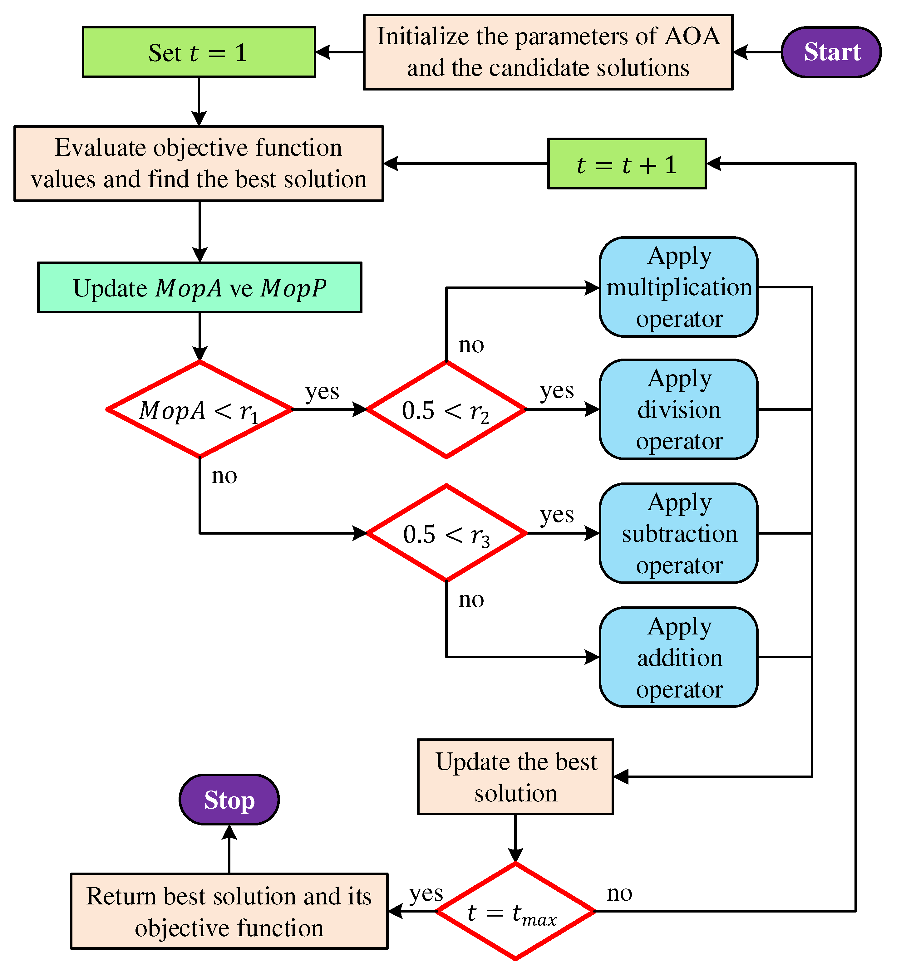
Figure 2.
Flowchart of pattern search method.
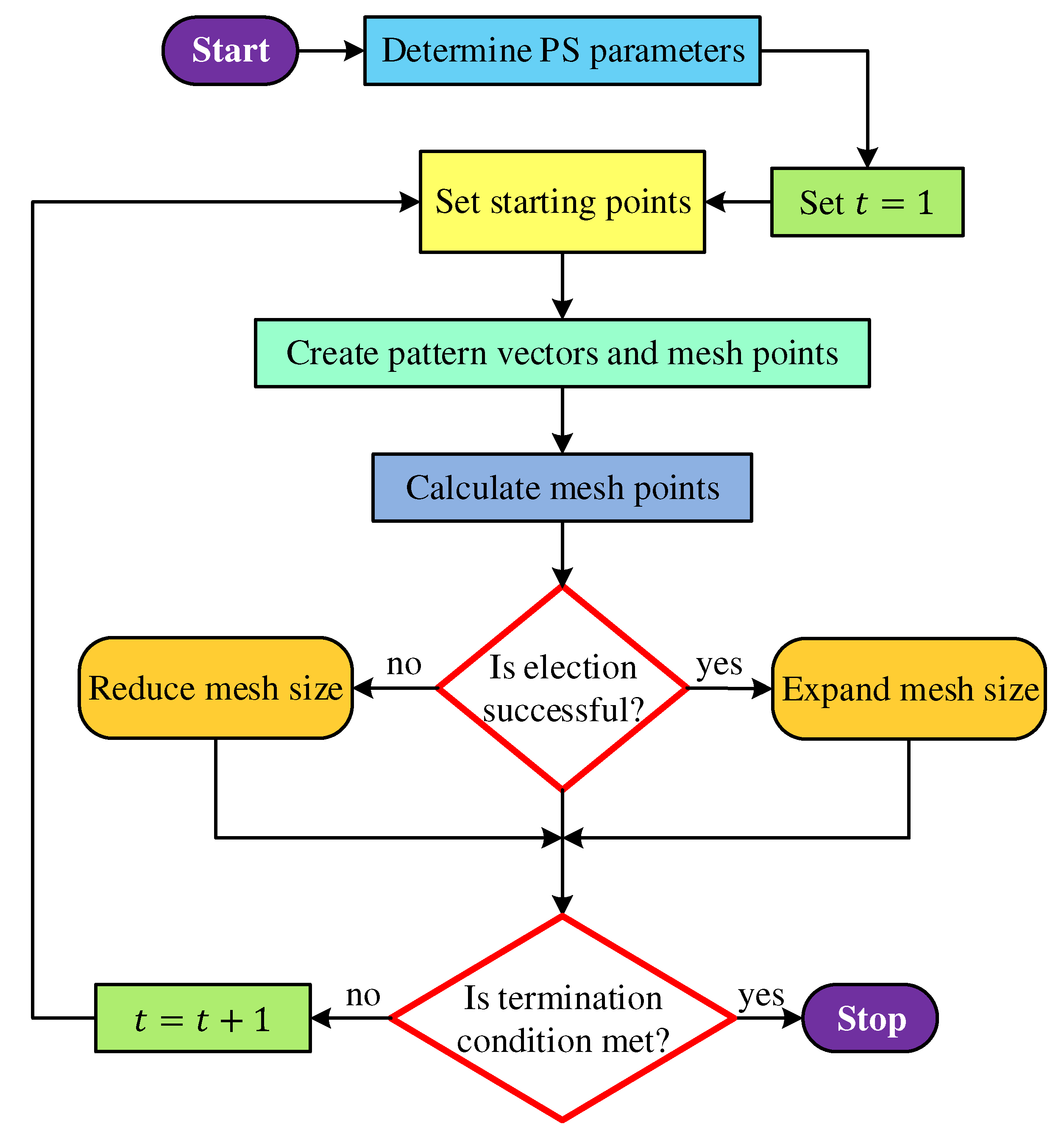
Figure 3.
Working principle of OBL mechanism.
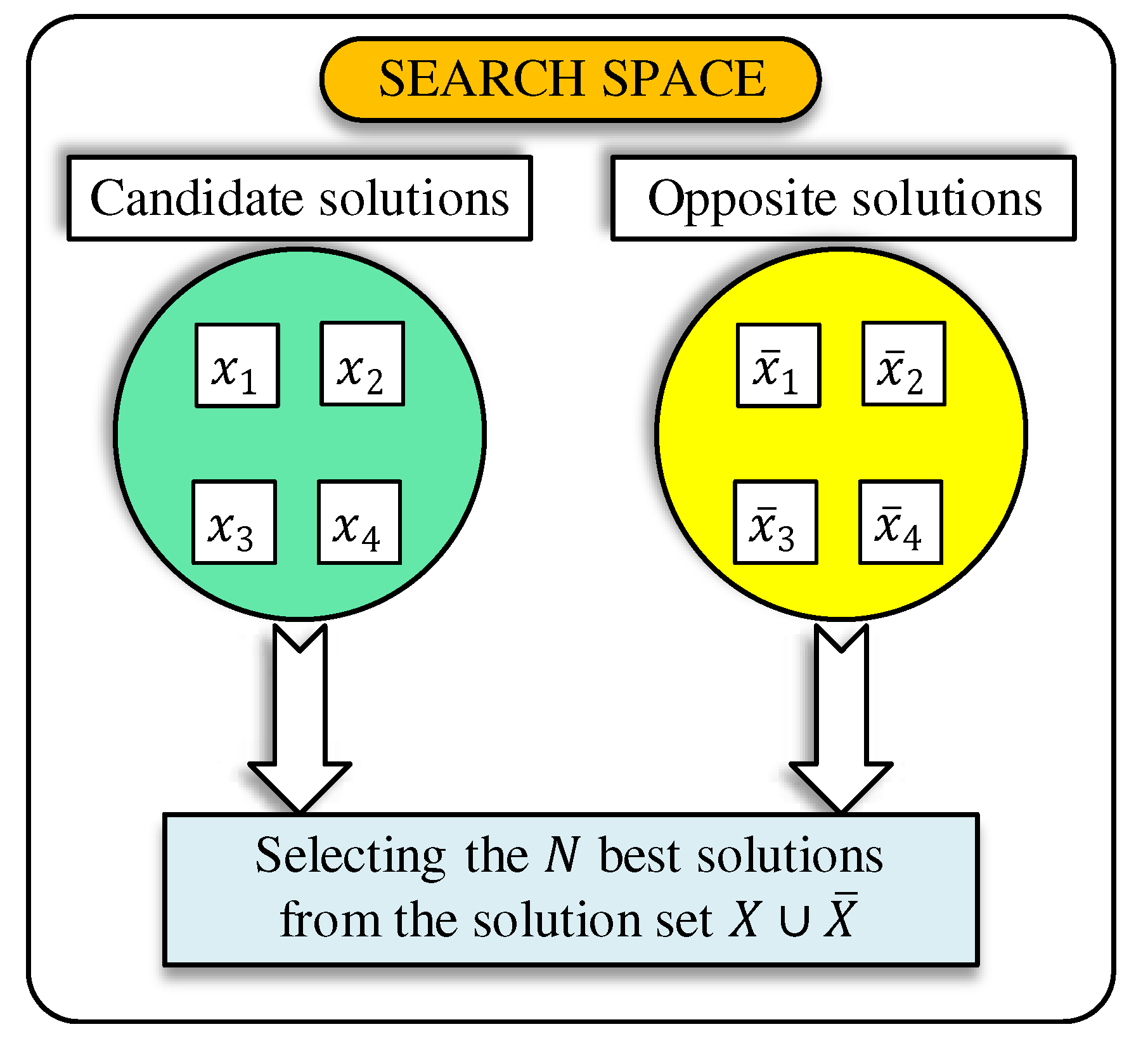
Figure 4.
Flowchart of proposed b-AOA algorithm.
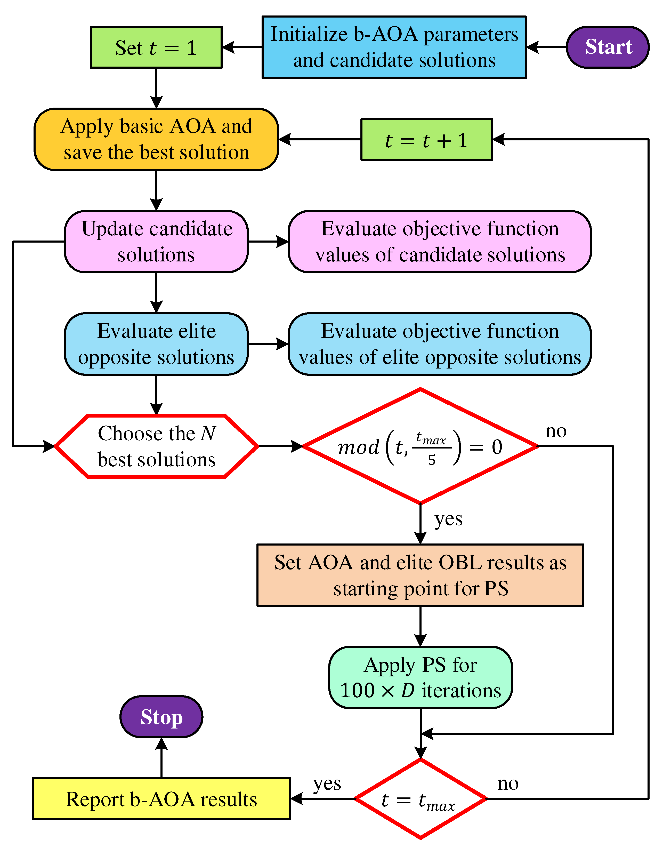
Figure 5.
Schematic diagram of a typical AVR system.
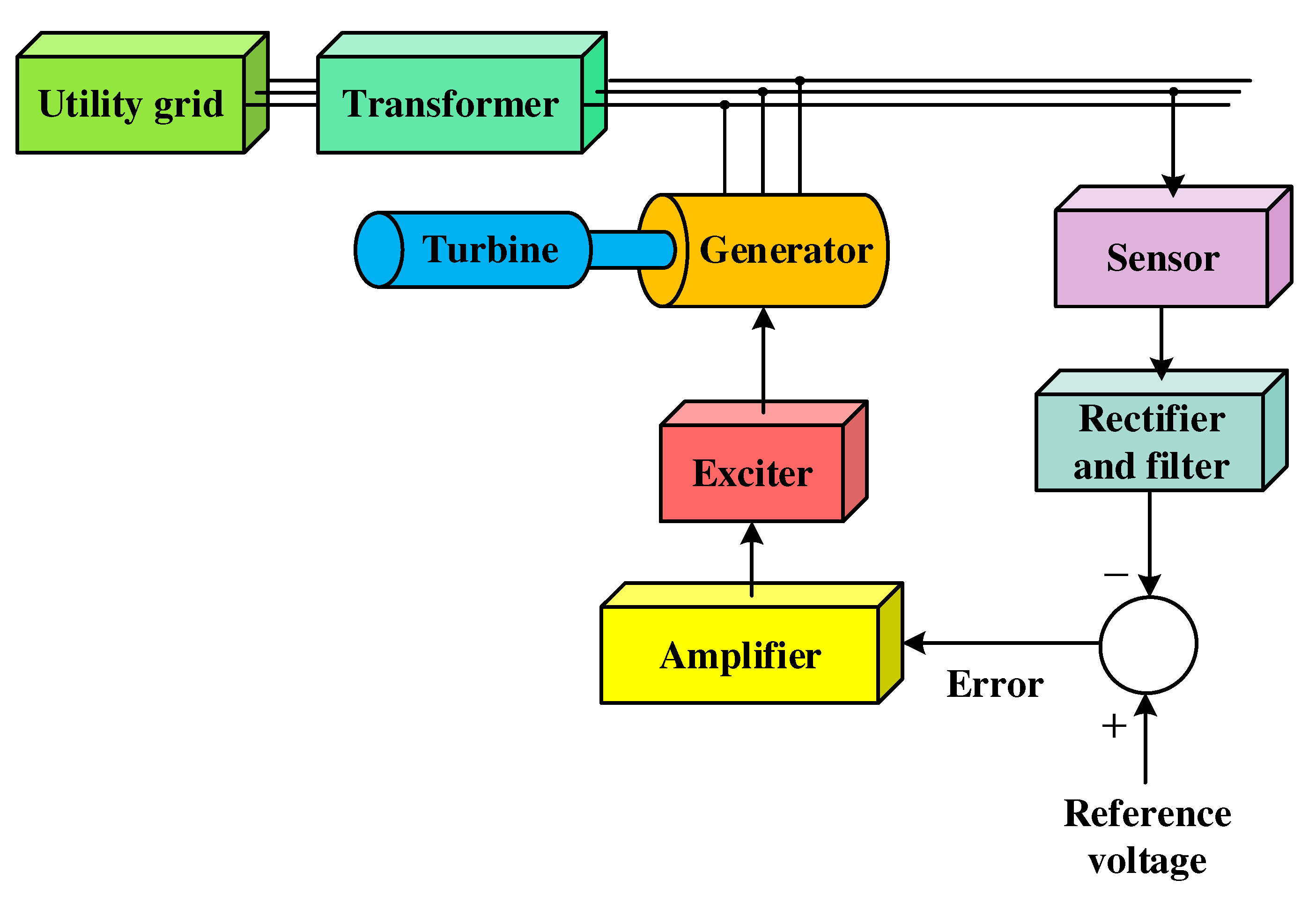
Figure 6.
An Uncontrolled AVR system.
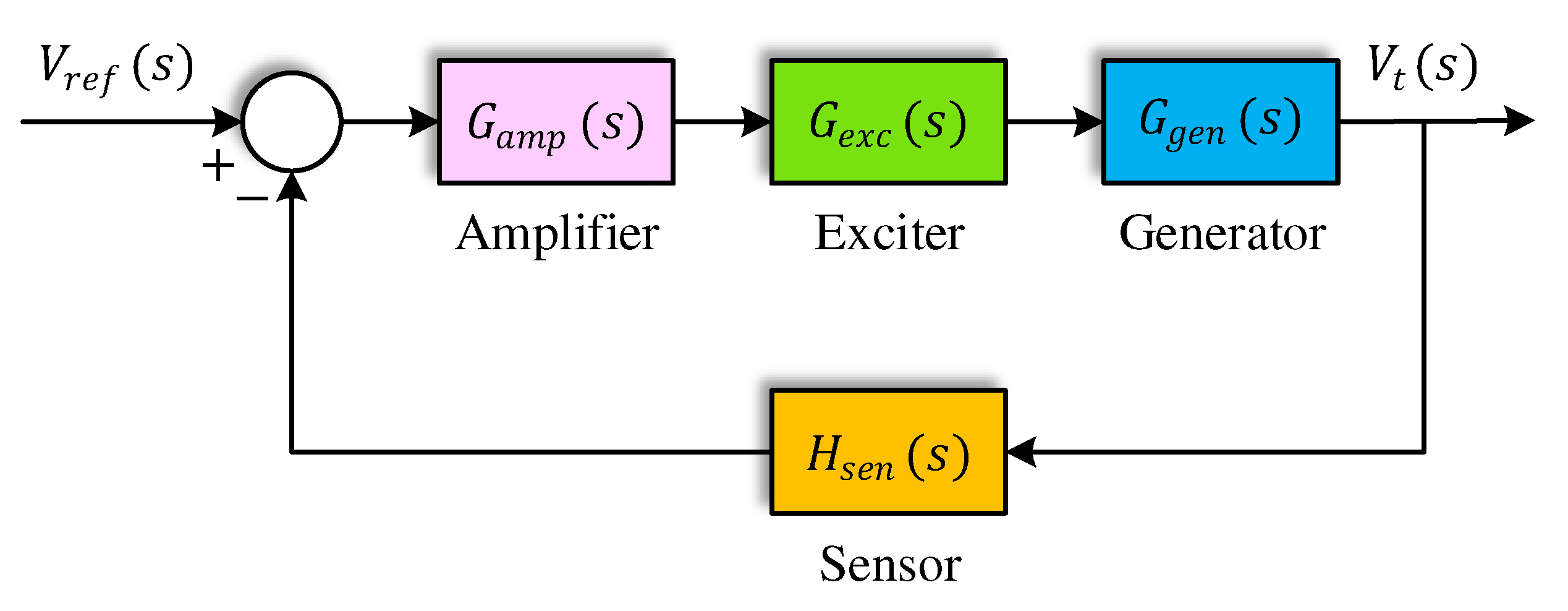
Figure 7.
Pole-zero map of uncontrolled AVR system.
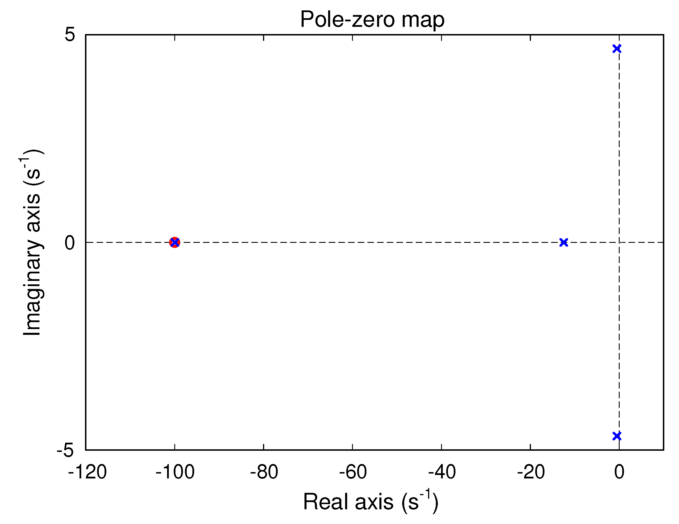
Figure 8.
Step response of the uncontrolled AVR system.
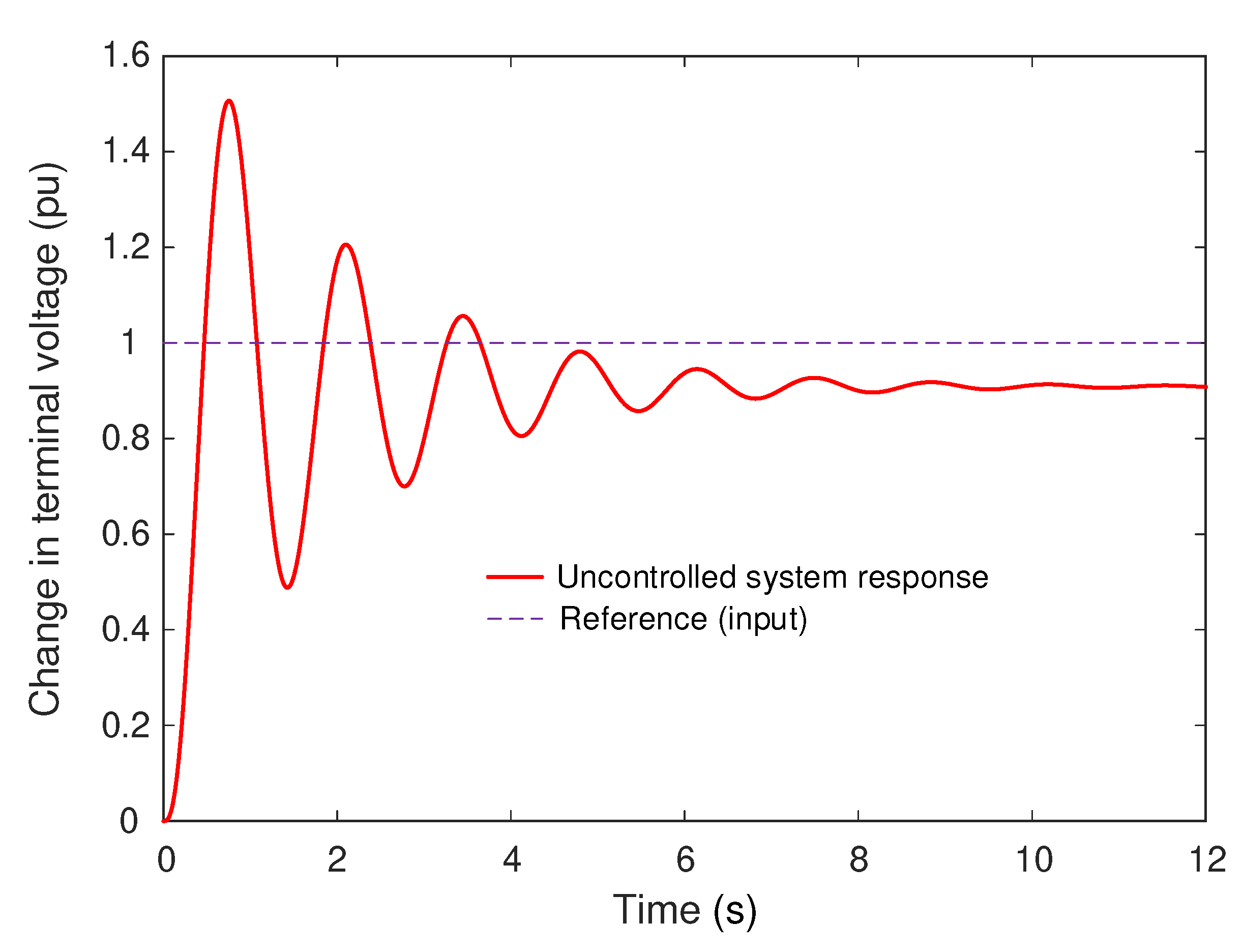
Figure 9.
Open loop Bode plot of the uncontrolled AVR system.
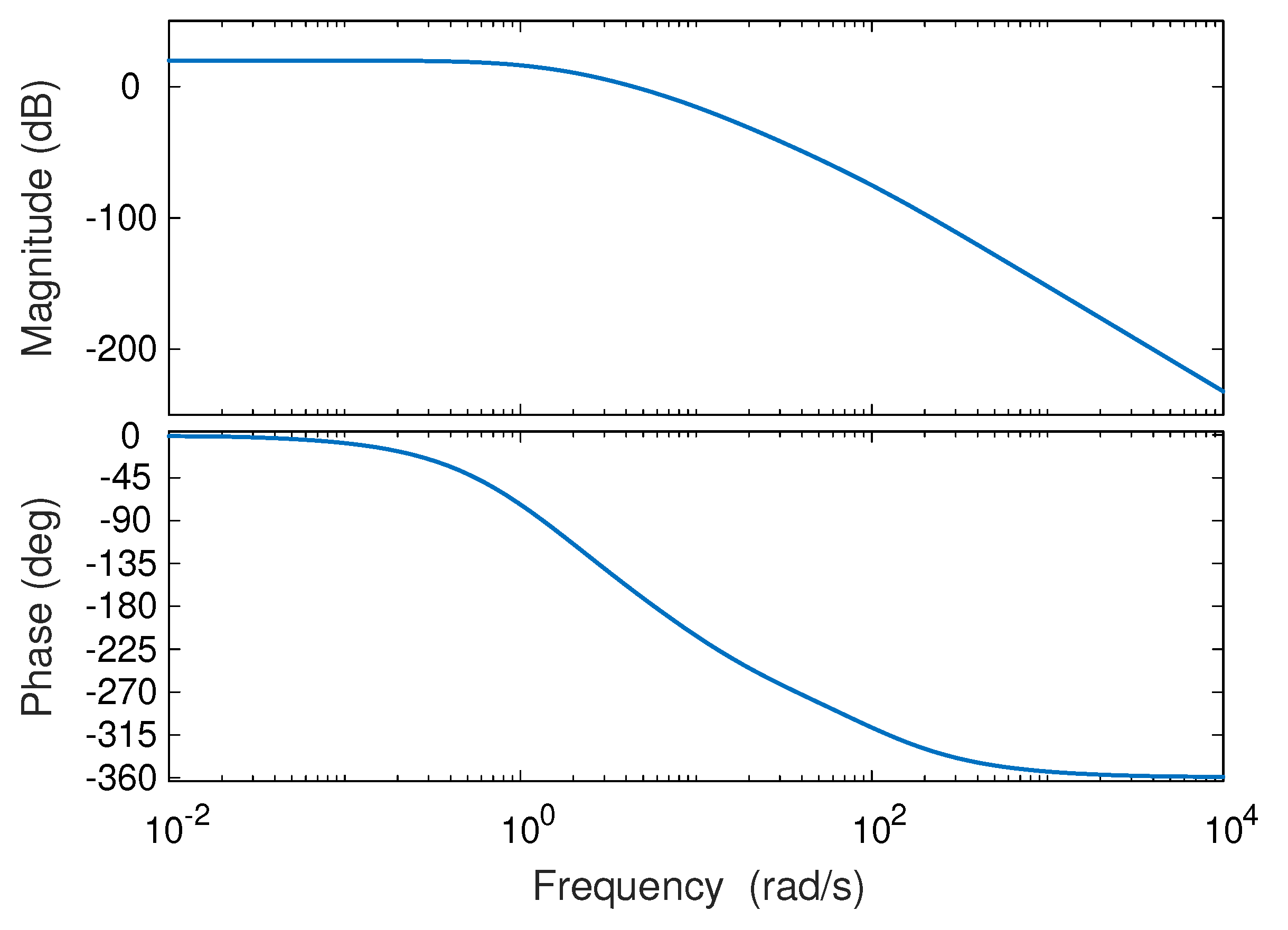
Figure 10.
Block diagram of PIDND2N2 controller.
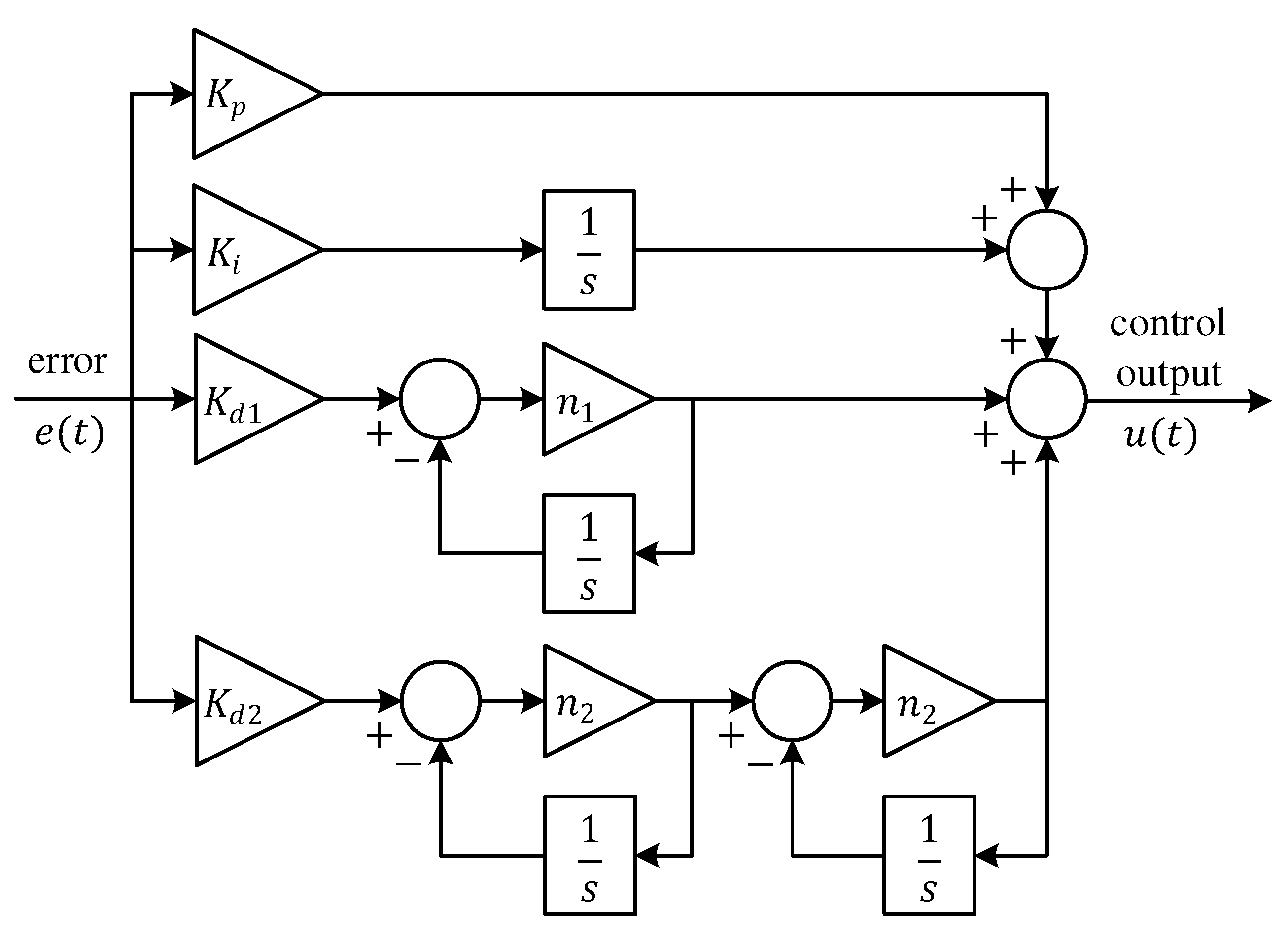
Figure 11.
The block diagram of the implementation of the proposed approach to AVR system.
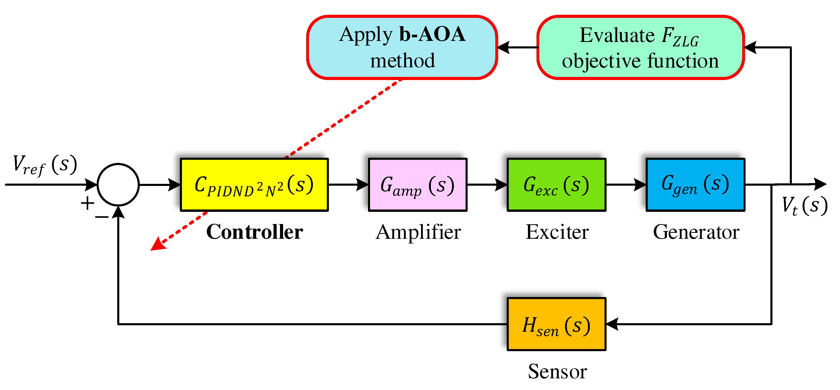
Figure 12.
Convergence curve for b-AOA and original AOA
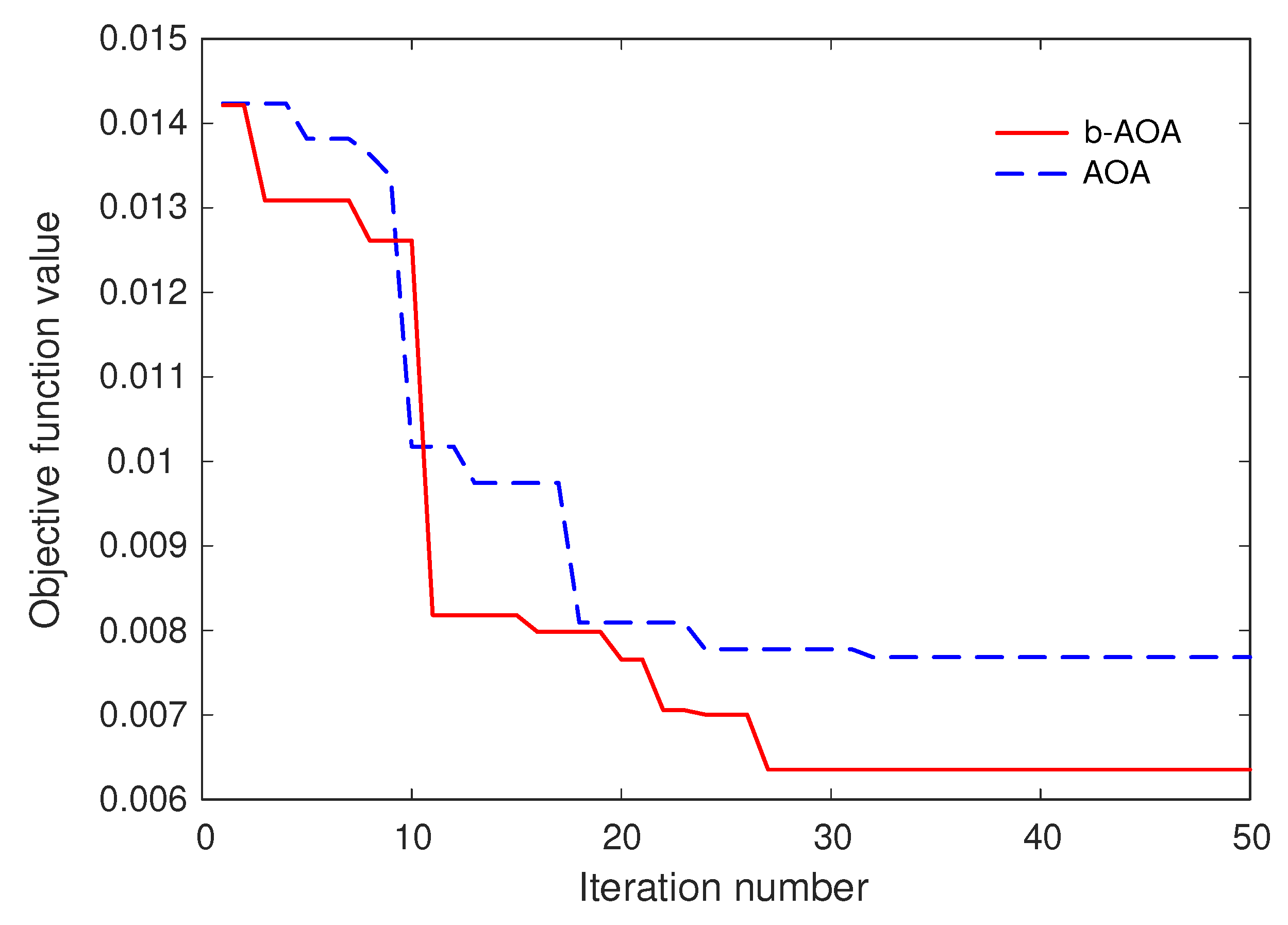
Figure 13.
Step response of b-AOA and AOA-tuned PIDND2N2 controllers for the change in the terminal voltage.
Figure 13.
Step response of b-AOA and AOA-tuned PIDND2N2 controllers for the change in the terminal voltage.
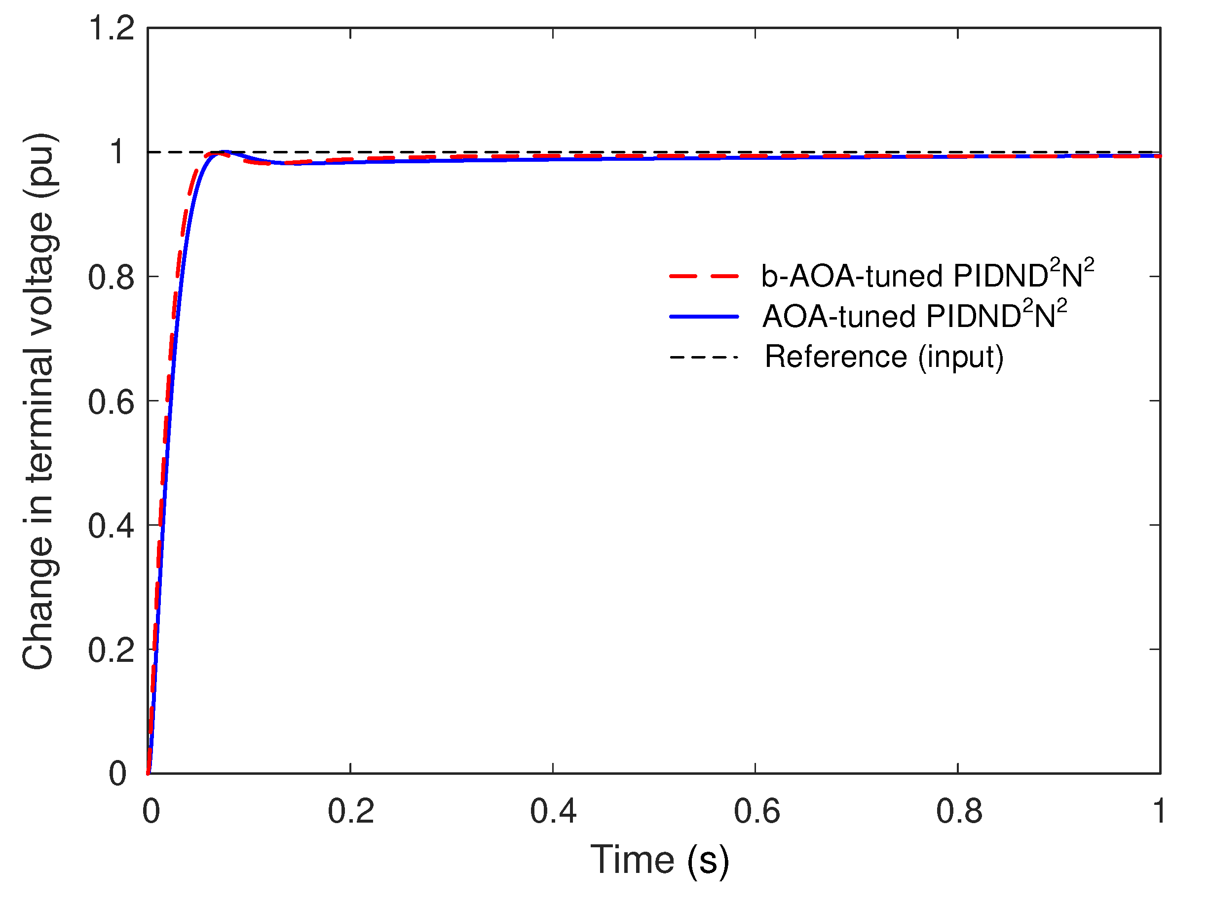
Figure 14.
Open loop Bode diagrams for b-AOA and AOA-tuned PIDND2N2 controllers
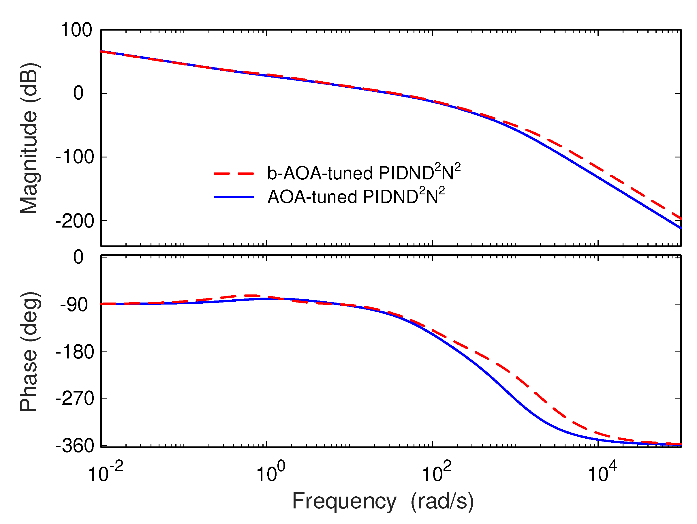
Figure 15.
Comparative step response of different control approaches for AVR system
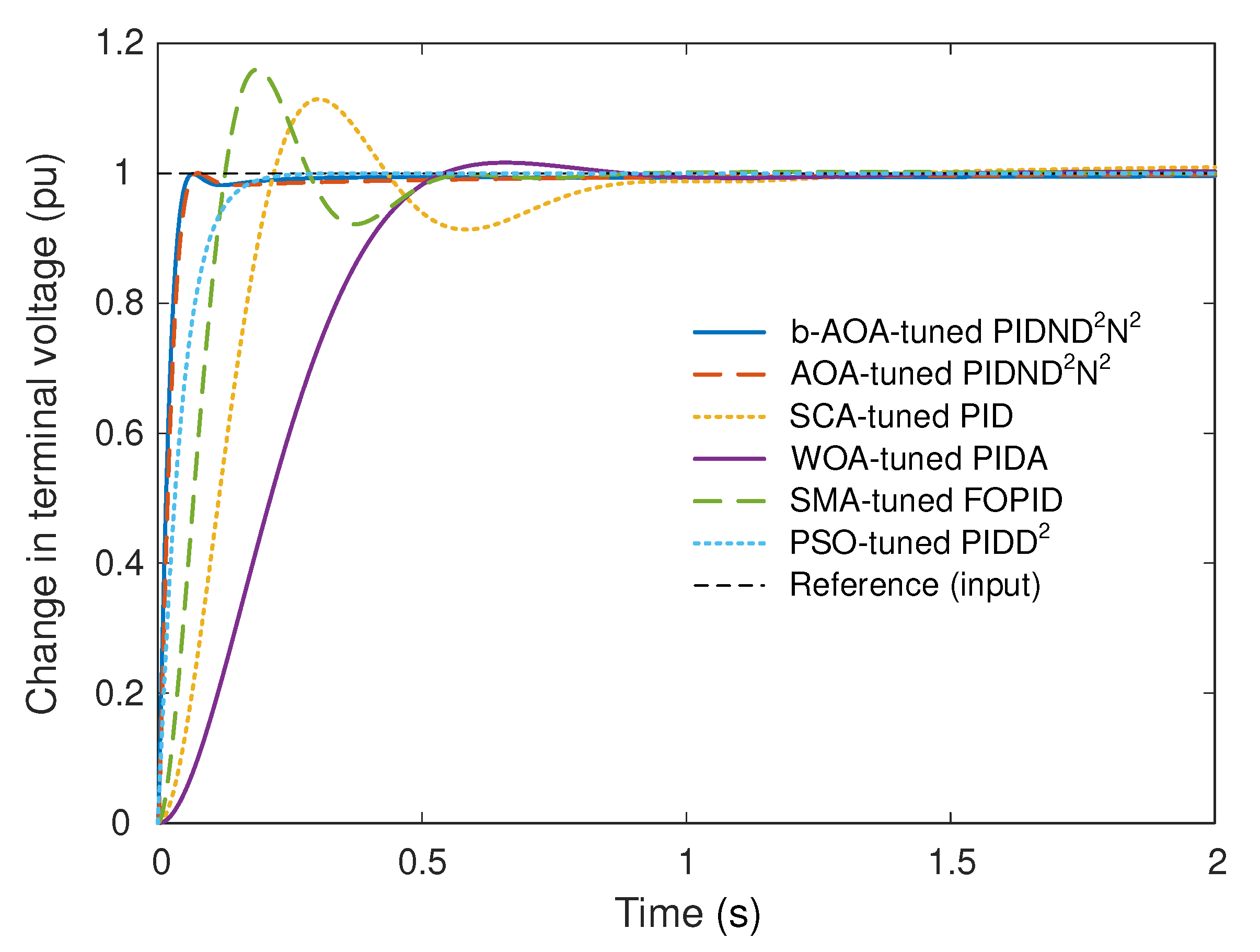
Figure 16.
Comparative Bode diagrams of different control approaches for AVR system
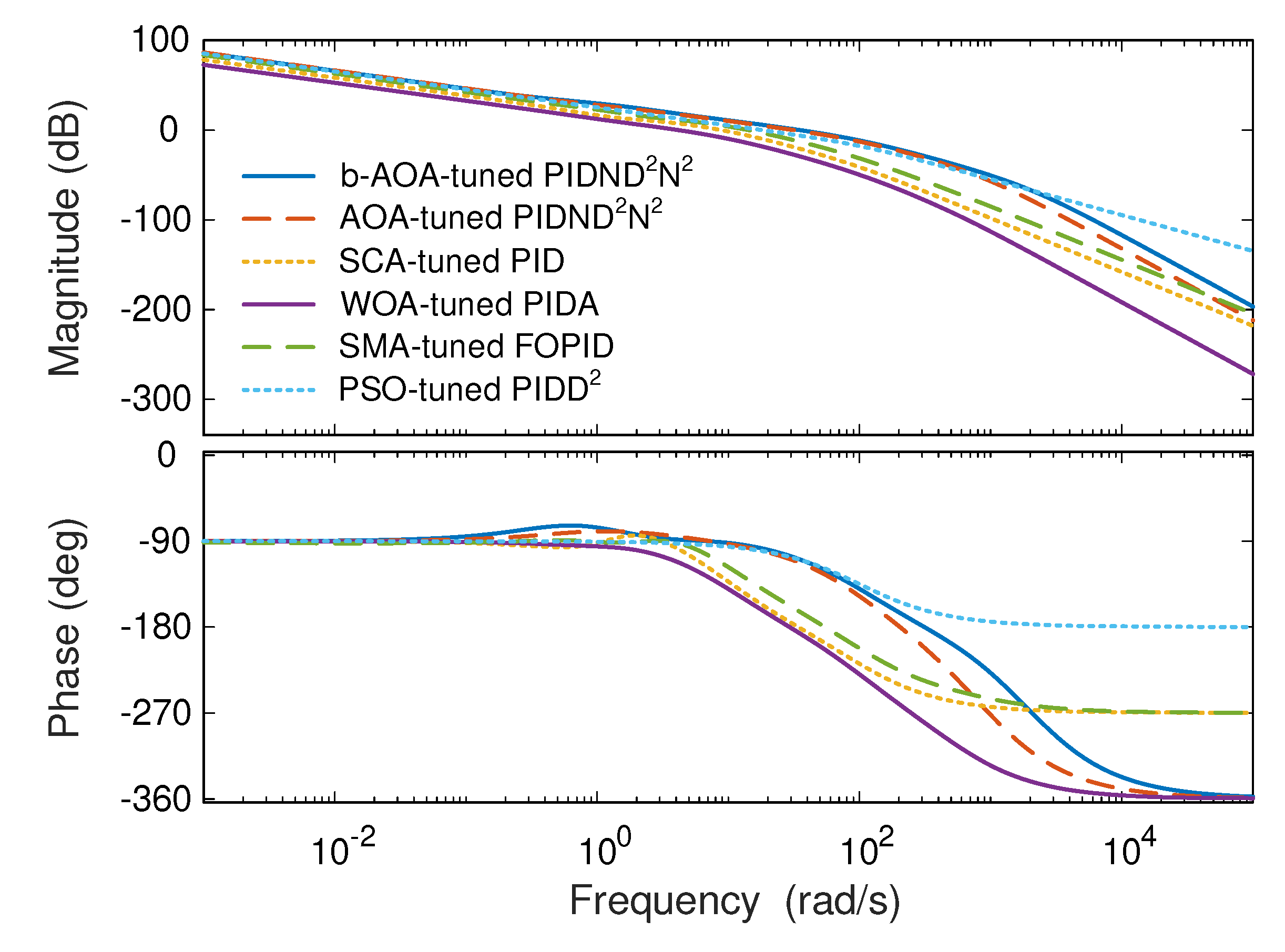

Table 1.
Properties of the adopted unimodal benchmark functions.
| Name | Function | Dimension | Evaluation interval | Global minimum |
|---|---|---|---|---|
| Sphere | 30 | 0 | ||
| Schwefel 2.2 | 30 | 0 | ||
| Schwefel 1.2 | 30 | 0 | ||
| Schwefel 2.21 | 30 | 0 | ||
| Rosenbrock | 30 | 0 | ||
| Step | 30 | 0 | ||
| Quartic | 30 | 0 |
Table 2.
Properties of the adopted multimodal benchmark functions.
| Name | Function | Dimension | Evaluation interval | Global minimum |
|---|---|---|---|---|
| Schwefel | 30 | −1.2569E+04 | ||
| Rastrigin | 30 | 0 | ||
| Ackley | 30 | 0 | ||
| Griewank | 30 | 0 | ||
| Penalized | 30 | 0 | ||
| Penalized2 | 30 | 0 |
Table 3.
Properties of the adopted fixed-dimensional multimodal benchmark functions.
| Name | Function | Dimension | Evaluation interval | Global minimum |
|---|---|---|---|---|
| Foxholes | 2 | 0.998 | ||
| Kowalik | 4 | 3.0749E−04 | ||
| Six-Hump Camel | 2 | −1.0316 | ||
| Branin | 2 | 0.39789 | ||
| Goldstein-Price | 2 | 3 | ||
| Hartman 3 | 3 | −3.8628 | ||
| Hartman 6 | 6 | −3.322 | ||
| Shekel 5 | 4 | −10.1532 | ||
| Shekel 7 | 4 | −10.4029 | ||
| Shekel 10 | 4 | −10.5364 |
Table 4.
Properties of the compared algorithms (population size, total iteration number, values of other control parameters).
Table 4.
Properties of the compared algorithms (population size, total iteration number, values of other control parameters).
| Algorithm | Population size | Total iteration number | Values of other control parameters |
|---|---|---|---|
| b-AOA | 30 | 500 | , , , , , , , |
| AOA [5] | 30 | 500 | , , , |
| SCA [19] | 30 | 500 | |
| INFO [20] | 30 | 500 | , |
| MPA [21] | 30 | 500 | , |
Table 5.
Comparative statistical results obtained from unimodal benchmark functions.
| Function | Algorithm | Mean | Standard Deviation | Best | Worst |
|---|---|---|---|---|---|
| b-AOA | 0 | 0 | 0 | 0 | |
| AOA | 0.00029656 | 0.0011413 | 3.9226E−38 | 0.0060134 | |
| SCA | 16.537 | 36.426 | 9.5633E−06 | 175.47 | |
| INFO | 1.0185E−53 | 4.997E−54 | 3.3545E−55 | 2.0178E−53 | |
| MPA | 4.0116E−23 | 6.3963E−23 | 3.6461E−25 | 2.7727E−22 | |
| b-AOA | 8.5996E−241 | 0 | 4.333E−320 | 2.2954E−239 | |
| AOA | 2.8674E−186 | 0 | 9.6235E−296 | 8.6022E−185 | |
| SCA | 0.021241 | 0.031567 | 0.00013767 | 0.13042 | |
| INFO | 1.0943E−26 | 3.6605E−27 | 4.7283E−27 | 1.9892E−26 | |
| MPA | 2.6444E−13 | 2.8514E−13 | 8.2406E−15 | 1.2622E−12 | |
| b-AOA | 0 | 0 | 0 | 0 | |
| AOA | 1.6011 | 3.3816 | 1.3815E−07 | 16.177 | |
| SCA | 8640.8 | 4939.5 | 1709.5 | 20103 | |
| INFO | 1.4606E−50 | 1.1602E−50 | 8.6654E−52 | 3.9712E−50 | |
| MPA | 9.9612E−05 | 0.00022346 | 7.2658E−09 | 0.001186 | |
| b-AOA | 9.0422E−244 | 0 | 1.2808E−253 | 2.6479E−242 | |
| AOA | 0.15416 | 0.094877 | 0.014632 | 0.36318 | |
| SCA | 37.033 | 13.087 | 12.166 | 61.964 | |
| INFO | 2.1028E−27 | 1.4215E−27 | 3.5852E−28 | 7.4954E−27 | |
| MPA | 2.7542E−09 | 1.5152E−09 | 3.1553E−10 | 6.0257E−09 | |
| b-AOA | 0.61615 | 1.8814 | 3.0737E−09 | 6.3967 | |
| AOA | 28.693 | 0.27549 | 27.902 | 29.18 | |
| SCA | 1.3673E+05 | 3.2682E+05 | 107.54 | 1175700 | |
| INFO | 22.585 | 0.51711 | 21.298 | 23.462 | |
| MPA | 25.268 | 0.45451 | 24.487 | 26.042 | |
| b-AOA | 2.4395E−12 | 9.2009E−13 | 1.086E−12 | 5.8521E−12 | |
| AOA | 3.7524 | 0.33331 | 3.0561 | 4.4582 | |
| SCA | 14.254 | 13.542 | 4.7191 | 55.025 | |
| INFO | 1.2654E−08 | 3.7987E−08 | 3.9266E−11 | 2.07E−07 | |
| MPA | 4.1868E−08 | 2.2575E−08 | 1.3296E−08 | 1.2965E−07 | |
| b-AOA | 3.629E−05 | 2.8489E−05 | 6.8524E−07 | 0.00010771 | |
| AOA | 9.4896E−05 | 7.1313E−05 | 2.0672E−06 | 0.00029718 | |
| SCA | 0.099158 | 0.090509 | 0.0085847 | 0.44986 | |
| INFO | 0.0015937 | 0.0012634 | 0.00017227 | 0.0049221 | |
| MPA | 0.0013495 | 0.00060352 | 0.00041966 | 0.0026601 |
Table 6.
Comparative statistical results obtained from multimodal benchmark functions.
| Function | Algorithm | Mean | Standard Deviation | Best | Worst |
|---|---|---|---|---|---|
| b-AOA | −12536 | 172.87 | −12569 | −11623 | |
| AOA | −7980.7 | 446.84 | −9196.5 | −7230.3 | |
| SCA | −3848.4 | 286.86 | −4371 | −3283.7 | |
| INFO | −8630.7 | 700.38 | −9763.3 | −7101.2 | |
| MPA | −8736.9 | 438.15 | −9687.9 | −7946.9 | |
| b-AOA | 0 | 0 | 0 | 0 | |
| AOA | 0 | 0 | 0 | 0 | |
| SCA | 29.308 | 30.189 | 0.13996 | 122.46 | |
| INFO | 0 | 0 | 0 | 0 | |
| MPA | 0 | 0 | 0 | 0 | |
| b-AOA | 8.8818E−16 | 0 | 8.8818E−16 | 8.8818E−16 | |
| AOA | 8.8818E−16 | 0 | 8.8818E−16 | 8.8818E−16 | |
| SCA | 14.208 | 8.3212 | 0.043401 | 20.382 | |
| INFO | 8.8818E−16 | 0 | 8.8818E−16 | 8.8818E−16 | |
| MPA | 1.7196E−12 | 1.1519E−12 | 2.7045E−13 | 5.8482E−12 | |
| b-AOA | 0 | 0 | 0 | 0 | |
| AOA | 194.12 | 65.896 | 72.408 | 323.52 | |
| SCA | 0.84569 | 0.41164 | 0.23545 | 1.9083 | |
| INFO | 0 | 0 | 0 | 0 | |
| MPA | 0 | 0 | 0 | 0 | |
| b-AOA | 2.1943E−13 | 1.5539E−13 | 5.0331E−14 | 6.0379E−13 | |
| AOA | 0.29154 | 0.053809 | 0.14538 | 0.43947 | |
| SCA | 52428 | 1.5261E+05 | 1.0947 | 614430 | |
| INFO | 1.4456E−09 | 2.8117E−09 | 5.3463E−12 | 1.1459E−08 | |
| MPA | 0.00014286 | 0.0005059 | 2.4157E−09 | 0.0023059 | |
| b-AOA | 3.1668E−12 | 2.4141E−12 | 7.6907E−13 | 9.0849E−12 | |
| AOA | 2.4484 | 0.16915 | 2.1217 | 2.8078 | |
| SCA | 1.0872E+05 | 2.7869E+05 | 2.2042 | 1305400 | |
| INFO | 0.063752 | 0.14273 | 3.2034E−10 | 0.69157 | |
| MPA | 0.012215 | 0.036876 | 2.8969E−08 | 0.19763 |
Table 7.
Comparative statistical results obtained from fixed-dimensional multimodal benchmark functions.
Table 7.
Comparative statistical results obtained from fixed-dimensional multimodal benchmark functions.
| Function | Algorithm | Mean | Standard Deviation | Best | Worst |
|---|---|---|---|---|---|
| b-AOA | 0.998 | 1.5701E−17 | 0.998 | 0.998 | |
| AOA | 8.3696 | 3.2389 | 0.998 | 12.671 | |
| SCA | 1.795 | 0.9859 | 0.998 | 2.9821 | |
| INFO | 2.1111 | 2.5903 | 0.998 | 10.763 | |
| MPA | 0.998 | 1.515E−16 | 0.998 | 0.998 | |
| b-AOA | 0.00030749 | 1.4923E−15 | 0.00030749 | 0.00030749 | |
| AOA | 0.015417 | 0.025604 | 0.00037189 | 0.11249 | |
| SCA | 0.0010661 | 0.00037002 | 0.0005829 | 0.0015477 | |
| INFO | 0.0024352 | 0.0060863 | 0.00030749 | 0.020363 | |
| MPA | 0.00030749 | 4.3122E−15 | 0.00030749 | 0.00030749 | |
| b-AOA | −1.0316 | 1.9902E−16 | −1.0316 | −1.0316 | |
| AOA | −1.0316 | 6.0816E−07 | −1.0316 | −1.0316 | |
| SCA | −1.0316 | 3.7905E−05 | −1.0316 | −1.0315 | |
| INFO | −1.0316 | 6.5843E−16 | −1.0316 | −1.0316 | |
| MPA | −1.0316 | 4.4024E−16 | −1.0316 | −1.0316 | |
| b-AOA | 0.39789 | 0 | 0.39789 | 0.39789 | |
| AOA | 0.40987 | 0.009864 | 0.39844 | 0.43767 | |
| SCA | 0.40026 | 0.0023543 | 0.39797 | 0.40949 | |
| INFO | 0.39789 | 0 | 0.39789 | 0.39789 | |
| MPA | 0.39789 | 9.5078E−15 | 0.39789 | 0.39789 | |
| b-AOA | 3 | 0 | 3 | 3 | |
| AOA | 6.6 | 9.3351 | 3 | 30 | |
| SCA | 3 | 5.4359E−05 | 3 | 3.0002 | |
| INFO | 3 | 8.6883E−16 | 3 | 3 | |
| MPA | 3 | 2.1709E−15 | 3 | 3 | |
| b-AOA | −3.8628 | 2.4116E−15 | −3.8628 | −3.8628 | |
| AOA | −3.8523 | 0.0038518 | −3.8593 | −3.842 | |
| SCA | −3.8547 | 0.0024361 | −3.861 | −3.8495 | |
| INFO | −3.8628 | 2.6823E−15 | −3.8628 | −3.8628 | |
| MPA | −3.8628 | 2.4945E−15 | −3.8628 | −3.8628 | |
| b-AOA | −3.322 | 2.1608E−13 | −3.322 | −3.322 | |
| AOA | −3.0471 | 0.091025 | −3.1762 | −2.8234 | |
| SCA | −2.8784 | 0.34163 | −3.1199 | −1.6747 | |
| INFO | −3.2784 | 0.058273 | −3.322 | −3.2031 | |
| MPA | −3.322 | 1.7554E−11 | −3.322 | −3.322 | |
| b-AOA | −10.153 | 7.6605E−13 | −10.153 | −10.153 | |
| AOA | −3.5023 | 1.1997 | −6.0307 | −1.8035 | |
| SCA | −2.6202 | 2.0715 | −7.8686 | −0.49728 | |
| INFO | −9.1039 | 2.4723 | −10.153 | −2.6305 | |
| MPA | −10.153 | 4.1471E−11 | −10.153 | −10.153 | |
| b-AOA | −10.403 | 1.1144E−12 | −10.403 | −10.403 | |
| AOA | −3.5619 | 1.2118 | −6.8762 | −1.4002 | |
| SCA | −3.2023 | 1.8303 | −5.9956 | −0.52105 | |
| INFO | −9.0488 | 2.7774 | −10.403 | −2.7659 | |
| MPA | −10.403 | 5.9857E−11 | −10.403 | −10.403 | |
| b-AOA | −10.536 | 3.2315E−12 | −10.536 | −10.536 | |
| AOA | −3.8733 | 1.6156 | −6.5892 | −1.5825 | |
| SCA | −3.7421 | 1.7935 | −6.1434 | −0.94135 | |
| INFO | −9.0039 | 3.151 | −10.536 | −2.4217 | |
| MPA | −10.536 | 2.5368E−11 | −10.536 | −10.536 |
Table 8.
Boundaries for PIDND2N2 Controller parameters.
| Bound | ||||||
|---|---|---|---|---|---|---|
| Lower | 0.001 | 0.001 | 0.001 | 0.001 | 50 | 50 |
| Upper | 5 | 5 | 5 | 5 | 2000 | 2000 |
Table 9.
Statistical performance of b-AOA and original AOA for AVR system.
| Algorithm | Mean | Standard Deviation | Best | Worst |
|---|---|---|---|---|
| b-AOA | 0.0065138 | 9.3497E−05 | 0.0063522 | 0.0067022 |
| AOA | 0.0078863 | 0.00012395 | 0.0076825 | 0.0081212 |
Table 10.
Optimal parameters of PIDND2N2 controller obtained via b-AOA and original AOA algorithms
| Optimized by | ||||||
|---|---|---|---|---|---|---|
| b-AOA | 4.8723 | 2.0240 | 1.8094 | 0.15049 | 1595.2 | 1971.2 |
| AOA | 3.9448 | 2.1188 | 1.6757 | 0.13014 | 1544.2 | 871.72 |
Table 11.
Transient response performance metrics for b-AOA and AOA-tuned PIDND2N2 controllers.
| Design method | Rise time (s) | Settling time (s) | Overshoot (%) |
|---|---|---|---|
| b-AOA-tuned PIDND2N2 | 0.033485 | 0.050752 | 0 |
| AOA-tuned PIDND2N2 | 0.037393 | 0.057523 | 0.043859 |
Table 12.
Frequency response performance metrics for b-AOA and AOA-tuned PIDND2N2 controllers.
| Design method | Phase margin (°) | Gain margin (dB) | Bandwidth (rad/s) |
|---|---|---|---|
| b-AOA-tuned PIDND2N2 | 70.797 | 28.888 | 64.820 |
| AOA-tuned PIDND2N2 | 69.810 | 23.368 | 57.819 |
Table 13.
Comparative numerical values for transient response of different control approaches.
| Design method | Rise time (s) | Settling time (s) | Overshoot (%) |
|---|---|---|---|
| b-AOA-tuned PIDND2N2 | 0.033485 | 0.050752 | 0 |
| AOA-tuned PIDND2N2 | 0.037393 | 0.057523 | 0.043859 |
| SCA-tuned PID [23] | 0.1472 | 0.84133 | 11.425 |
| WOA-tuned PIDA [24] | 0.32772 | 0.49543 | 1.6483 |
| SMA-tuned FOPID [25] | 0.087541 | 0.4979 | 15.998 |
| PSO-tuned PIDD2 [26] | 0.092935 | 0.16347 | 0.0025797 |
Table 14.
Comparative numerical values for frequency response of different control approaches.
| Design method | Phase margin (°) | Gain margin (dB) | Bandwidth (rad/s) |
|---|---|---|---|
| b-AOA-tuned PIDND2N2 | 70.797 | 28.888 | 64.820 |
| AOA-tuned PIDND2N2 | 69.810 | 23.368 | 57.819 |
| SCA-tuned PID [33] | 52.596 | 20.300 | 14.821 |
| WOA-tuned PIDA [34] | 67.671 | 26.123 | 6.7076 |
| SMA-tuned FOPID [35] | 49.142 | 20.193 | 23.914 |
| PSO-tuned PIDD2 [36] | 79.638 | Infinite | 23.503 |
Table 15.
Transient response performance of the proposed approach with respect to recently reported other efficient methods.
Table 15.
Transient response performance of the proposed approach with respect to recently reported other efficient methods.
| Ref. | Year | Used controller type | Tuning method | Rise time (s) | Settling time (s) | Overshoot (%) |
|---|---|---|---|---|---|---|
| Proposed | PIDND2N2 | b-AOA | 0.033485 | 0.050752 | 0 | |
| [27] | 2023 | FOPID | MPA | 0.0833 | 0.1106 | 0.55 |
| [28] | PID | h-ASPSO | 0.3097 | 0.4679 | 1.2476 | |
| [44] | TIλDND2N2 | EO | 0.03752 | 0.0596 | 0.4128 | |
| [6] | FOPIDD2 | RSA | 0.0487 | 0.0806 | 0 | |
| [29] | 2022 | PIDND2N2 | iRUN | 0.0399 | 0.0626 | 0 |
| [30] | PID-F | SOS | 0.267 | 0.371 | 0.007 | |
| [31] | 2DOF fractional-order PI | WOA | 1.12 | 1.74 | 1.17 | |
| [32] | PID | L-RSANM | 0.3076 | 0.4669 | 0.9582 | |
| [15] | FOPID | ChBWO | 0.1103 | 0.169 | 1.1838 | |
| [33] | Fuzzy PID | GA | 0.1857 | 0.2963 | 1.0407 | |
| [34] | 2021 | FOPID with fractional filter | SCA | 0.1230 | 0.1670 | 0.1262 |
| [35] | PIDD2 | SA-MRFO | 0.0535 | 0.0798 | 0.7562 | |
| [14] | PID | SMA | 0.3149 | 0.4817 | 0.6071 | |
| [36] | FOPID | GBO | 0.0885 | 0.653 | 11.3 | |
| [37] | Sigmoid PID | NSCA | 0.498 | 0.579 | 2.2 | |
Disclaimer/Publisher’s Note: The statements, opinions and data contained in all publications are solely those of the individual author(s) and contributor(s) and not of MDPI and/or the editor(s). MDPI and/or the editor(s) disclaim responsibility for any injury to people or property resulting from any ideas, methods, instructions or products referred to in the content. |
© 2023 by the authors. Licensee MDPI, Basel, Switzerland. This article is an open access article distributed under the terms and conditions of the Creative Commons Attribution (CC BY) license (http://creativecommons.org/licenses/by/4.0/).
Copyright: This open access article is published under a Creative Commons CC BY 4.0 license, which permit the free download, distribution, and reuse, provided that the author and preprint are cited in any reuse.


