
Submitted:
18 July 2025
Posted:
21 July 2025
You are already at the latest version
Abstract
(1) Background: Multi-Objective Optimization is a prominent research area, in which approaches for the simultaneous solution of multiple objectives are proposed. The possibility to discover a set of parameters optimizing all the goals can be achieved only if the considered problems are rather trivial, while compromise solutions are generally discovered. Things become even more complex when the set of parameters is used in opposite, and potentially conflicting, ways. (2) Methods: in this work, we compared some state-of-the-art Evolutionary Algorithms with regard to the optimization of different conflicting objectives, by highlighting strengths and weaknesses of the different approaches. In particular, we considered four benchmark problems — 4-bit parity, double-pole balancing, grid navigation and test function optimization — to be solved simultaneously. (3) Results: our investigation identifies the algorithms leading to a better optimization. Moreover, we provide an analysis of the solutions to the single objectives, hence illustrating how the different methods address the problems. (4) Conclusions: two algorithms emerge as the most suitable methods for dealing with the considered scenario. Notably, a relatively simple strategy is not significantly inferior to a more sophisticated one, thus emphasizing that there exists a non-negligible relationship between problems and algorithms, and discovering general methods is extremely difficult.
Keywords:
multi-objective optimization
; neural networks
; evolutionary algorithms
; benchmarking
1. Introduction
Multi-Objective Optimization (MOO) [1] is a fascinating research field in which the ultimate goal consists of discovering solutions fulfilling multiple, often conflicting, objectives simultaneously [1]. Since the task is extremely complex or even impossible, compromise solutions are taken into account, which are referred to as Pareto-optimal [2]. By definition, a Pareto-optimal solution is “a set of ’non-inferior’ solutions in the objective space defining a boundary beyond which none of the objectives can be improved without sacrificing at least one of the other objectives” [3]. An illustration of the concept of Pareto optimality is provided in Figure 1.
Several techniques have been proposed to solve MOO problems, such as Evolutionary Algorithms (EAs) [4,5,6], Genetic Algorithms (GAs) [7,8,9] or swarm intelligence approaches [10,11,12]. For example, the authors in [13] applied GAs to discover Pareto-optimal solutions for a Supply Chain Network (SCN) design problem. Their analysis indicates the feasibility of the approach in the context of a Turkish company producing plastic products. Applications of GAs to MOO of test functions can be found in [14,15,16]. In [17,18], the OpenAI Evolutionary Strategy (OpenAI-ES) [19] has been used to cope with a MOO problem requiring a swarm of AntBullet robots [20] to simultaneously locomote and aggregate: the authors show that robots develop a good locomotion capability, while aggregation is obtained very rarely. This underscores the difficulty of optimizing both objectives at the same time.
Specific algorithms have been developed to address MOO with regard to test function optimization, such as Multi Objective Genetic Algorithm (MOGA) [21], Niched Pareto Genetic Algorithm (NPGA) [22], Nondominated Sorting Genetic Algorithm II (NSGA-II) [23] and Vector Evaluated Genetic Algorithm (VEGA) [24]. In particular, NSGA-II [23] enables to discover optimized solutions for test functions defined in [24,25] by exploiting non-dominated sorting, diversity-preservation and elitism combined with typical mutation and crossover operators from GAs. VEGA [24] represents a variant of a classic GA tailored for MOO scenarios. Specifically, the solution evaluation produces a vector of fitness values, one for each objective, and selection is made by choosing non-dominated solutions according to Pareto optimality. To this end, the whole population is split into sub-populations (one for each objective) from which the best individuals are selected. Finally, recombination and mutation of selected solutions allow to generate the new population and ensure diversity.
An interesting field related to MOO involves the discovery of effective controllers to manage different problems belonging to the same class. For example, the authors in [26] propose an approach called Shared Modular Policy (SMP) in which a global policy is used to control different modular neural networks. In particular, each module is responsible for the control of a single actuator based on current sensory readings and shared information in the form of current reward function. Experiments performed on robot locomotors characterized by diverse morphologies (e.g., Halfcheetah, Hopper, Humanoid, Walker2D) demonstrate the validity of the approach and a good generalization capability on new morphologies. Another worthwhile example can be found in [27], in which the authors propose an approach to discover a single controller for a class of dynamical systems. Specifically, through in-context learning [28], the authors demonstrate that an effective controller for a specific numerical problem can be immediately applied to a different problem within the same class, with no need for fine-tuning.
This work is halfway between MOO and the evolution of a single controller for multiple problems. In more detail, we present a comparative study of four EAs — Generational Genetic Algorithm (GGA) [29], OpenAI-ES [19], Stochastic Steady State [30] and Stochastic Steady State with Hill-Climbing (SSSHC) [31] — that must discover a single neural network controller capable to minimize simultaneously four benchmark problems: (i) 4-bit parity, (ii) double-pole balancing, (iii) grid navigation and (iv) test function optimization. Although using methods specifically tailored for MOO scenarios like NSGA-II or VEGA could be rather intuitive, we decided instead to put emphasis on the usage of general and relatively simple EAs [32] to assess how effective they are at sampling the search space and discovering optimized solutions for the MOO scenario. Moreover, the considered algorithms proved successful with respect to the benchmark problems addressed in isolation [30,31,33,34,35,36,37]. Our results clearly demonstrate that OpenAI-ES and SSSHC outperform GGA and SSS thanks to their propensity to reduce the size of weights, which is pivotal in the considered scenario. Furthermore, detailed analysis of the performance on the individual benchmark problems reveal that all the algorithms focus mainly on the minimization of test functions, which allows to quickly optimize performance. Interestingly, SSSHC achieves better performance than OpenAI-ES with respect to grid navigation and test function optimization, while the opposite is true for 4-bit parity and double-pole balancing. This implies that relatively simple strategies can perform similarly to more sophisticated algorithms.
The key contributions of this research are listed as follows:
- a new MOO scenario is introduced, which entails benchmark problems like 4-bit parity, double-pole balancing, grid navigation and test function optimization;
- a comparison of some state-of-the-art EAs on the defined MOO scenario is proposed;
- OpenAI-ES and SSSHC emerge as more effective than GGA and SSS at dealing with the novel MOO scenario;
- SSSHC outperforms OpenAI-ES with respect to grid navigation and test function optimization, while the opposite is true for 4-bit parity and double-pole balancing;
- OpenAI-ES has an intrinsic propensity to reduce the size of weights/parameters, which is paramount to discover effective solutions in the considered domain;
- the definition of the MOO scenario highlights the existence of a non-negligible relationship between problems and algorithms.
The paper starts with a thorough description of the benchmark problems, the considered EAs, the neural network controller and the experimental settings in Section 2. Then, a detailed illustration of the outcomes is provided in Section 3, which are further discussed in Section 4. Finally, Section 5 reports the main findings and potential future research ideas.
2. Materials and Methods
This section contains a description of the experimental problems that have been considered, as well as the evolutionary algorithms, the neural network controller, the simulator and the parameter settings used to perform the experiments.
2.1. Problems
2.1.1. 4-Bit Parity
The first problem is the 4-bit parity task, which consists in calculating the number of 1-bits in the input string and returning a value checking if the sum of 1-bits is even (output is 1) or odd (output is 0). The problem is illustrated in Figure 2 and is a commonly used task in the evolutionary computation literature [38,39,40,41,42].
Specifically, our evaluation is made by considering all the possible 4-bit input strings (i.e., ) and verifying the number of correct parity values returned. The fitness function is defined as in Eq. 1.
In Eq. 1, the symbol is the expected parity output for the input string s, indicates the output returned by the controller and represents the number of considered 4-bit input strings ().
2.1.2. Double-Pole Balancing
The second problem is the double-pole balancing task [37], a widespread benchmark to assess an algorithm performance as demonstrated by the large body of literature in the field [30,43,44,45,46,47]. The task involves the presence of two poles placed on the top of a wheeled mobile cart, which has to move properly to avoid poles falling (see Figure 3). The description of the parameters characterizing the problem is reported in Table 1.
The objective function of the problem can be formulated as in Eq. 2.
Symbol denotes the length of a trial (), in Eq. 2 represents the number of steps the cart keeps both poles upright during the trial i, whereas indicates the number of trials. An episode is prematurely ended in two cases:
- the cart goes out of the track ();
- the pole angles are falling (, with ).
In this work, we focus on the “Fixed Initial States condition” version of the problem [30,31], in which the evaluation of possible solutions is averaged over 8 trials (). In more detail, at each trial the state variables (x: position of the cart, : angle of the pole j, with ) are initialized according to Table 2.
2.1.3. Grid Navigation
The third problem is a grid navigation task in which an agent has to reach the central location (target) of a square grid starting from one of the four corners (see Figure 4). The grid has size . Similarly to the afore-described problems, grid navigation represents a largely used benchmark to evaluate genetic and evolutionary algorithms [48,49,50,51].
The objective/fitness function considers the distance between the target location and the final agent location, as expressed in Eq. 3.
In Eq. 3, the symbol indicates the final agent-target distance at the trial i and counts the number of trials. Since there are four possible starting locations (i.e., the corners of the grid), we set . The target-agent distance is calculated by considering the minimum number of cells the agent has to visit in order to arrive at the target, and is defined in Eq. 4.
The symbols and denote, respectively, the location of the target and the agent during the trial i.
The agent can move one cell either horizontally (i.e., left and right) or vertically (i.e., up and down) within the grid. A trial prematurely stops if the action of the agent causes its exit from the grid.
2.1.4. Test Function Optimization
The last problem is test function optimization, which constitutes a common benchmark for evaluating optimization methods [23,31,34,52,53,54,55]. In particular, we consider five different test functions: Ackley [56], Griewank [57], Rastrigin [58], Rosenbrock [59] and Sphere. Eqs. 5 - 9 provide the definition of the considered functions, in which the input sequence is identified with the symbol v and its length with the symbol n.
The fitness function for test function optimization is defined as the sum of the single functions according to Eq. 10.
2.2. Performance
To assess the overall performance of the discovered solutions with respect to the considered MOO scenario, we adopt the fitness function described in Eqs. 11 - 12:
As concerns Eq. 12, we use coefficients equal to 1.0 for each objective (i.e., ). Despite the simplicity of the approach, our design choice alleviates from the burden of choosing tailored values, which requires expertise and may lead to different evolutionary paths.
2.3. Evolutionary Algorithms
The EAs employed in this work are described in the next sections. A comprehensive schematic is provided in Figure 5. Further details about the different algorithms can be found in [19,29,30,31].
We emphasize that the term “solution” represents a set of floating-point values (also called “genes”) directly encoding the parameters (i.e., biases and connection weights) of the controller that must be evolved.
2.3.1. GGA
The Generational Genetic Algorithm (GGA) [29] is a pioneering method to evolve solutions capable of adapting to dynamic environments [60,61]. Moreover, it has been largely used in collective domains like Swarm Robotics [62,63,64,65,66] or Multi-Agent Systems (MASs) [67,68,69,70,71,72], as well as for problems involving single agents [73,74,75,76].
The algorithm works according to the schematic provided in Figure 5-(a): a population of candidate solutions is evolved until a termination criterion is not met. Each solution undergoes an evaluation process returning a fitness value rating its effectiveness. After the entire population has been evaluated, the best solutions are selected for reproduction, each one generating offspring through mutation and asexual crossover operators. Moreover, selected solutions are retained in the population through elitism. This iterative process aims to enhance the efficacy of solutions during evolution.
2.3.2. OpenAI-ES
The OpenAI Evolutionary Strategy (OpenAI-ES) [19] is a relatively novel technique that achieved competitive results in problems like Atari games [19], classic control [33,35], competitive co-evolution [77], robot locomotion [19,33,78] and swarm robotics [79,80,81]. Differently from a traditional EA, OpenAI-ES evolves a single solution termed “centroid”. In particular, at each iteration of the evolutionary process, samples are extracted from a Gaussian distribution and a set of solutions are derived according to Eq. 13.
In Eq. 13, the symbol s represents the generic sample, c denotes the centroid, and indicate the solutions that undergo evaluation, while is the mutation rate.
Once the pool of solutions has been evaluated, a fitness ranking is used to estimate the gradient of the expected fitness function. Finally, the centroid is updated through Adam [82], a widespread optimizer keeping historical information to drive the search process towards solutions that are more likely to be effective. A schematic of OpenAI-ES is shown in Figure 5-(b). Differently from existing works [19,33,78,79,80], here OpenAI-ES does not exploit weight decay [83], since reducing the size of weights represents a clear advantage in the considered MOO scenario.
2.3.3. SSS
The Stochastic Steady State (SSS) [30] is an EA that found applications in problems like double-pole balancing [30,31,34,84], swarm robotics [84,85], car racing games [84] and Pybullet robot locomotors [86]. The algorithm differs from GGA with respect to the reproduction and selection process: at each iteration, each solution in the population (parent) generates one offspring through mutation and asexual crossover. Then, both parents and offspring are evaluated and the best solutions are retained and form the next population. This iterative process allows SSS to improve performance during evolution. Figure 5-(c) provides a schematic of the operation of SSS.
2.3.4. SSSHC
The Stochastic Steady State with Hill-Climbing (SSSHC) [31] is a memetic algorithm [87,88,89] combining SSS with a Hill-Climbing algorithm [90] seeking to further refine the solution performance. SSSHC proves successful with regard to problems such as 5-bit parity, double-pole balancing and test function optimization [31,34]. Specifically, for the experiments reported here, we used the variant introduced in [34].
The operation of SSSHC follows the one of SSS, but a refinement phase is added after selection: each selected solution undergoes iterations in which a single gene mutation is applied and the modified solution is retained only if its performance improves. A description of SSSHC is illustrated in Figure 5-(d).
2.4. Controller
As a single controller for the considered problems, we used a recurrent neural network [91,92] formed by 4 inputs, an internal layer of 10 neurons, and 1 output. Bias is applied to internal and output neurons, which activate based on the tanh function. The information the input and output neurons encode depending on the specific problem is listed here below (see also Table 3).
- 4-bit parity: the inputs represent the bits of the string that has to be checked, while the output is the parity value associated to the string;
- double-pole balancing: the inputs encode normalized values for the cart position (x) and pole angles ( and ), and an alert signal that activates if either the cart approaches track edges (), or the poles are almost falling (, with ). The output represents the force that will be exerted to the cart;
- grid navigation: the inputs are the normalized locations of the agent () and the target (), whereas the output indicates the motion direction (i.e., left, up, right or bottom).
Regarding test function optimization, the connection weights of the neural network constitute the input vector v used to compute the functions in Eq. 5 - 9. Therefore, not only does the controller have to optimize simultaneously four problems exhibiting different properties, but it also has to address them in potentially conflicting ways. In fact, the latter problem requires to minimize the size of connection weights, which could prevent the discovery of effective solutions for the other problems.
2.5. Simulator and Experimental Settings
The Framework for Autonomous Robotics Simulation and Analysis (FARSA) [93] tool has been employed for the experiments reported in this work, since it found applications in similar experimental studies [30,31,34]. Moreover, it has been successfully used also in robotic scenarios [76,85,94,95].
The considered EAs have been compared by running 30 replications of the experiments. Evolution last evaluation steps for each algorithm in order to provide a fair comparison. Other parameter settings are reported in Table 4.
3. Results
The performance comparison is shown in Table 5, Figure 6 and Figure 7. Clearly, OpenAI-ES and SSSHC strongly outperform GGA and SSS (Kruskal-Wallis H test, , see Table 6), which indicates their capability to discover more effective solutions for the considered MOO scenario. As can be seen in Figure 6, OpenAI-ES and SSSHC quickly reduce the fitness in the first evaluation steps and then almost stabilize after evaluation steps. This implies that both algorithms manage to identify the direction in the search space corresponding to an optimized performance. Conversely, the fitness curves of GGA and SSS show a slower drop, which prevents them from further optimization.
Notably, OpenAI-ES and SSSHC have similar performance (Mann-Whitney U test, , see also Figure 7 and Table 6). Therefore, a relatively simple strategy like SSSHC is not inferior to a more sophisticated algorithm like OpenAI-ES, which exploits historical information to channel the search in the space of possible solutions. By looking at the outcomes reported in Figure 7, OpenAI-ES manages to find solutions with performance below 1000 (see bottom outliers in Figure 7), while SSSHC does not reach similar performance levels.
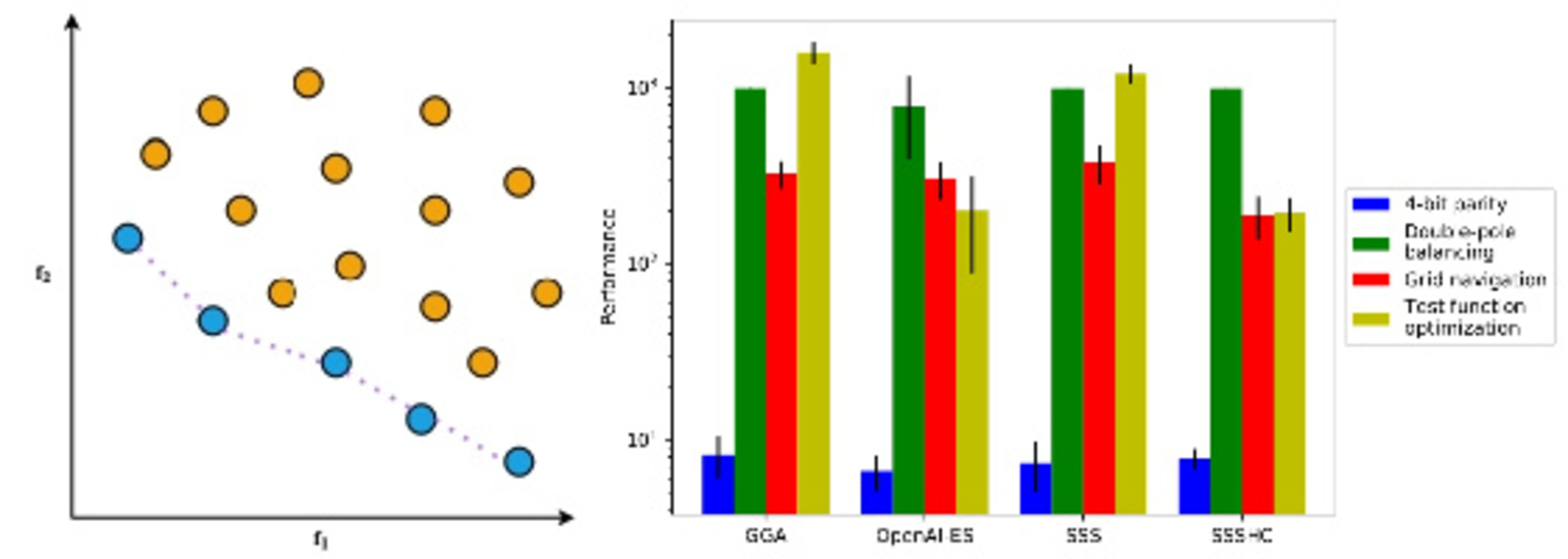
We corroborate our results by delving into the fitness achieved by the different algorithms with regard to the specific problems. As highlighted in Figure 8 and Table 7, OpenAI-ES achieves the best results in the 4-bit parity and double-pole balancing problems, while SSSHC bests other algorithms with respect to grid navigation and test function optimization. In particular, OpenAI-ES and SSSHC succeed in the minimization of test functions, which allows to quickly reduce fitness (see also Figure 6). Instead, GGA and SSS fail in finding similar solutions. Furthermore, SSSHC is notably superior to the other algorithms in the grid navigation problem (Kruskal-Wallis H test, ). Interestingly, OpenAI-ES is the only algorithm that manages to discover improved solutions in the double-pole balancing problem (Kruskal-Wallis H test, , see also Figure 8 and Table 7).
Lastly, we investigate the performance of the different algorithms with respect to Ackley, Griewank, Rastrigin, Rosenbrock and Sphere functions, as illustrated in Figure 9 and Table 8. Notably, OpenAI-ES is more effective than other algorithms in optimizing the Rosenbrock function (Kruskal-Wallis H test, ), whereas SSSHC bests other algorithms with respect to the remaining four test functions (Kruskal-Wallis H test, ). GGA and SSS achieve poor performance in this context, particularly concerning the Rosenbrock function (see Table 8).
Overall, the reported analysis clearly reveals a superior performance of OpenAI-ES and SSSHC over GGA and SSS. This is related to their capability to decrease weights, as shown in Table 9. In particular, the former algorithms evolve controllers with a limited weight size, which is paramount for the test function optimization. Nevertheless, this tendency prevents the algorithms from finding effective solutions with respect to the other problems, particularly double-pole balancing. This is especially true for SSSHC (see Figure 8 and Table 7). OpenAI-ES and SSS have similar weight sizes, but their performance is notably different. This can be explained by considering that OpenAI-ES exploits historical information to effectively sample the search space, while SSS does not adopt similar mechanisms.
4. Discussion
The presented results show that two algorithms emerge as more suitable options for the considered MOO scenario. A noteworthy aspect regards the different level of complexity between OpenAI-ES and SSSHC. In fact, the former method exploits mirrored sampling [96] and historical information to identify the search direction in the space of solutions. Conversely, SSSHC is a memetic algorithm that seeks to refine selected solutions through single gene mutations. Despite the simplicity, SSSHC works well in this scenario. However, the approach presents benefits and drawbacks: on one hand, modifying one gene at a time eliminates the risk of disruptive effects, since only adaptive mutations are retained. On the other hand, the process does not exclude failures in the attempt of improving solution performance and is costly in terms of number of evaluation steps.
OpenAI-ES has an intrinsic propensity to reduce the size of weights even when weight decay is not applied, as in the case of our experiments. This turns out to be crucial in the considered domain, as well as in other domains like robot locomotion [33] and swarm robotics [80]. Conversely, SSSHC exploits single gene mutations performed during refinement to progressively reduce the weight size.
GGA and SSS do not manage to achieve performance comparable to the other algorithms. Specifically, they fail in discovering effective solutions for test function optimization, particularly with respect to the Rosenbrock function. This can be explained by considering that both GGA and SSS seek to enhance performance through mutation and crossover operators, and do not have explicit techniques to reduce weights. As a consequence, they might require longer evolutionary processes in order to find more effective solutions.
Another relevant insight concerns the types of solutions discovered by the considered EAs. In particular, we observe that all the algorithms mainly focus on test function optimization, which allows to quickly enhance performance, and almost ignore the remaining problems. This is strongly related to the remarkable different magnitudes of the fitness values in the worst case (see Table 10): because test function optimization is three order of magnitude bigger than double-pole balancing and grid navigation, the fitness function defined in Eq. 12 is minimized when the component is strongly reduced. As a consequence, the algorithms evolve solutions mostly addressing test function optimization and do not manage to improve performance with respect to the other objectives.
Overall, our results underscore a non-negligible relationship between problem and algorithm. In fact, although OpenAI-ES, SSS and SSSHC proved effective at optimizing double-pole balancing in previous studies [30,31,33,35], the definition of the performance measure for the considered MOO scenario guides EAs to different evolutionary paths, in which one of the objectives dominate the others.
5. Conclusions
Multi-Objective Optimization (MOO) concerns the identification of solutions capable of optimizing multiple conflicting objectives at the same time. Because the discovery of a global optimum is not trivial, if not impossible, Pareto-optimal solutions are typically taken into account. Evolutionary Algorithms (EAs) have demonstrated a great ability to deal with MOO scenarios, since they provide effective solutions without any prior knowledge about the considered domains. A partially related research field lies in the search for a single controller able to address different problems within the same class. The main advantage is the possibility of transferring acquired knowledge on a given problem to others, without further fine-tuning. The approach is similar to transfer learning [97], which proved valuable in Deep Learning (DL) applications [98,99,100].
This work delves into the definition of a novel MOO scenario and the analysis of how some state-of-the-art works address it. Specifically, we compared GGA, OpenAI-ES, SSS and SSSHC with respect to the evolution of a single neural network controller able to simultaneously optimize four benchmark problems: (i) 4-bit parity, (ii) double-pole balancing, (iii) grid navigation, and (iv) test function optimization. The definition of the scenario makes the overall problem challenging, since the multiple objectives conflict with each other. Furthermore, the controller is used differently depending on the specific problem: for example, the connection weights determine the action to be executed in the double-pole balancing or grid navigation problems, while they represent the input vector for the test functions to be optimized. Outcomes indicate that OpenAI-ES and SSSHC best the other algorithms, since they are more effective at sampling the search space. In particular, OpenAI-ES exploits symmetric sampling and historical information, whereas SSSHC benefits from single-gene mutations. Interestingly, a relatively trivial algorithm like SSSHC is not inferior to a modern and sophisticated method like OpenAI-ES in this context. Instead, SSSHC is better than OpenAI-ES with respect to grid navigation and test function optimization, while the opposite is true for 4-bit parity and double-pole balancing. In addition, OpenAI-ES and SSSHC manage to reduce weight size more efficiently than GGA and SSS, a worthwhile feature in the considered domain.
As future research directions, we plan to incorporate algorithms specifically tailored for MOO domains, such as NSGA-II and VEGA, for future comparisons. This will provide a comprehensive analysis of the most suitable methods for MOO. Furthermore, modifications of the problem formulation in Eq. 12 will be object of future studies, particularly through either the usage of different coefficient values for the different objectives, or the normalization of the fitness functions defined in Eqs. 1, 2, 3 and 10. In addition, further experiments in which parameter settings are systematically varied will be performed, aiming to validate our analysis more thoroughly. Finally, future works could investigate different scenarios (e.g., robotics, classic control) in order to extend and, possibly, generalize the considerations reported here.
Funding
This research received no external funding.
Data Availability Statement
Code for replicating the experiments can be found at https://github.com/PaoloP84/SingleControllerForMultipleTasks.
Conflicts of Interest
The authors declare no conflicts of interest.
References
- Deb, K.; Sindhya, K.; Hakanen, J. Multi-objective optimization. In Decision sciences; CRC Press, 2016; pp. 161–200.
- Censor, Y. Pareto optimality in multiobjective problems. Applied Mathematics and Optimization 1977, 4, 41–59. [Google Scholar] [CrossRef]
- Kara, N.; Köçken, H.G. An Approach for a Multi-Objective Capacitated Transportation Problem. In Encyclopedia of Data Science and Machine Learning; IGI Global, 2023; pp. 2385–2399.
- Deb, K. Multi-objective optimisation using evolutionary algorithms: an introduction. In Multi-objective evolutionary optimisation for product design and manufacturing; Springer, 2011; pp. 3–34.
- Fonseca, C.M.; Fleming, P.J. An overview of evolutionary algorithms in multiobjective optimization. Evolutionary computation 1995, 3, 1–16. [Google Scholar] [CrossRef]
- Tan, K.C.; Lee, T.H.; Khor, E.F. Evolutionary algorithms for multi-objective optimization: Performance assessments and comparisons. Artificial intelligence review 2002, 17, 251–290. [Google Scholar] [CrossRef]
- Chafekar, D.; Xuan, J.; Rasheed, K. Constrained multi-objective optimization using steady state genetic algorithms. In Proceedings of the Genetic and evolutionary computation conference. Springer, 2003, pp. 813–824.
- Coello, C.A.C.; Lamont, G.B.; Van Veldhuizen, D.A. Evolutionary algorithms for solving multi-objective problems; Springer, 2007.
- Konak, A.; Coit, D.W.; Smith, A.E. Multi-objective optimization using genetic algorithms: A tutorial. Reliability engineering & system safety 2006, 91, 992–1007. [Google Scholar] [CrossRef]
- Alaya, I.; Solnon, C.; Ghedira, K. Ant colony optimization for multi-objective optimization problems. In Proceedings of the 19th IEEE international conference on tools with artificial intelligence (ICTAI 2007). IEEE, 2007, Vol. 1, pp. 450–457.
- Janga Reddy, M.; Nagesh Kumar, D. An efficient multi-objective optimization algorithm based on swarm intelligence for engineering design. Engineering Optimization 2007, 39, 49–68. [Google Scholar] [CrossRef]
- Yasear, S.A.; Ku-Mahamud, K.R. Review of the multi-objective swarm intelligence optimization algorithms. Journal of Information and Communication Technology 2021, 20, 171–211. [Google Scholar] [CrossRef]
- Altiparmak, F.; Gen, M.; Lin, L.; Paksoy, T. A genetic algorithm approach for multi-objective optimization of supply chain networks. Computers & industrial engineering 2006, 51, 196–215. [Google Scholar] [CrossRef]
- Gao, Y.; Shi, L.; Yao, P. Study on multi-objective genetic algorithm. In Proceedings of the 3rd World Congress on Intelligent Control and Automation. IEEE, 2000, Vol. 1, pp. 646–650.
- Jin, Y.; Sendhoff, B. Constructing dynamic optimization test problems using the multi-objective optimization concept. In Proceedings of the Workshops on Applications of Evolutionary Computation. Springer, 2004, pp. 525–536.
- Okabe, T.; Jin, Y.; Olhofer, M.; Sendhoff, B. On test functions for evolutionary multi-objective optimization. In Proceedings of the International Conference on Parallel Problem Solving from Nature. Springer, 2004, pp. 792–802.
- Pagliuca, P.; Vitanza, A. Enhancing Aggregation in Locomotor Multi-Agent Systems: a Theoretical Framework. Proceedings of the 25th Edition of the Workshop From Object to Agents (WOA24) 2024, 3735, 42–57.
- Pagliuca, P.; Trivisano, G.; Vitanza, A. How to Evolve Aggregation in Robotic Multi-Agent Systems. Proceedings of the 26th Edition of the Workshop From Object to Agents (WOA25) 2025.
- Salimans, T.; Ho, J.; Chen, X.; Sidor, S.; Sutskever, I. Evolution strategies as a scalable alternative to reinforcement learning. arXiv preprint arXiv:1703.03864 2017.
- Coumans, E.; Bai, Y. Pybullet, a python module for physics simulation for games, robotics and machine learning, 2016.
- Murata, T.; Ishibuchi, H. MOGA: multi-objective genetic algorithms. In Proceedings of the IEEE international conference on evolutionary computation. IEEE Piscataway, 1995, Vol. 1, pp. 289–294.
- Horn, J.; Nafpliotis, N.; Goldberg, D.E. A niched Pareto genetic algorithm for multiobjective optimization. In Proceedings of the First IEEE conference on evolutionary computation. IEEE world congress on computational intelligence. Ieee, 1994, pp. 82–87.
- Deb, K.; Pratap, A.; Agarwal, S.; Meyarivan, T. A fast and elitist multiobjective genetic algorithm: NSGA-II. IEEE transactions on evolutionary computation 2002, 6, 182–197. [Google Scholar] [CrossRef]
- Schaffer, J.D. Multiple objective optimization with vector evaluated genetic algorithms. In Proceedings of the First international conference on genetic algorithms and their applications. Psychology Press, 2014, pp. 93–100.
- Fonseca, C.M.; Fleming, P.J. Multiobjective optimization and multiple constraint handling with evolutionary algorithms. II. Application example. IEEE Transactions on systems, man, and cybernetics-Part A: Systems and humans 2002, 28, 38–47. [Google Scholar] [CrossRef]
- Huang, W.; Mordatch, I.; Pathak, D. One policy to control them all: Shared modular policies for agent-agnostic control. In Proceedings of the International Conference on Machine Learning. PMLR, 2020, pp. 4455–4464.
- Busetto, R.; Breschi, V.; Forgione, M.; Piga, D.; Formentin, S. One controller to rule them all. Proceedings of Machine Learning Research 2025, 1, 14. [Google Scholar]
- Dong, Q.; Li, L.; Dai, D.; Zheng, C.; Ma, J.; Li, R.; Xia, H.; Xu, J.; Wu, Z.; Liu, T.; et al. A survey on in-context learning. arXiv preprint arXiv:2301.00234 2022. [CrossRef]
- Grefenstette, J.J. Genetic algorithms for changing environments. In Proceedings of the International Conference on Parallel Problem Solving From Nature (PPSN), 1992, Vol. 2, pp. 137–144.
- Pagliuca, P.; Milano, N.; Nolfi, S. Maximizing adaptive power in neuroevolution. PLOS ONE 2018, 13, 1–27. [Google Scholar] [CrossRef] [PubMed]
- Pagliuca, P. Learning and evolution: factors influencing an effective combination. AI 2024, 5, 2393–2432. [Google Scholar] [CrossRef]
- Back, T. Evolutionary algorithms in theory and practice: evolution strategies, evolutionary programming, genetic algorithms; Oxford university press, 1996.
- Pagliuca, P.; Milano, N.; Nolfi, S. Efficacy of modern neuro-evolutionary strategies for continuous control optimization. Frontiers in Robotics and AI 2020, 7, 98. [Google Scholar] [CrossRef] [PubMed]
- Pagliuca, P. Analysis of the Exploration-Exploitation Dilemma in Neutral Problems with Evolutionary Algorithms. Journal of Artificial Intelligence and Autonomous Intelligence 2024, 1, 8. [Google Scholar] [CrossRef]
- Pagliuca, P.; Nolfi, S.; Vitanza, A. Evorobotpy3: a flexible and easy-to-use simulation tool for Evolutionary Robotics. In Proceedings of the Proceedings of the Genetic and Evolutionary Computation Conference (GECCO 2025 Companion), 2025.
- Reis, C.; Machado, J.; Cunha, J.B. Logic circuits synthesis through genetic algorithms. WSEAS Transactions on Information Science and Applications 2005, 2, 618–623. [Google Scholar]
- Wieland, A.P. Evolving neural network controllers for unstable systems. In Proceedings of the International Joint Conference on Neural Networks (IJCNN). IEEE, 1991, Vol. 2, pp. 667–673.
- Chandra, R.; Gupta, A.; Ong, Y.S.; Goh, C.K. Evolutionary multi-task learning for modular training of feedforward neural networks. In Proceedings of the Neural Information Processing: 23rd International Conference, ICONIP 2016, Kyoto, Japan, October 16–21, 2016, Proceedings, Part II 23. Springer, 2016, pp. 37–46.
- Hohmann, S.G.; Schemmel, J.; Schürmann, F.; Meier, K. Exploring the parameter space of a genetic algorithm for training an analog neural network. In Proceedings of the 4th Annual Conference on Genetic and Evolutionary Computation, 2002, pp. 375–382.
- Liu, D.; Hohil, M.E.; Smith, S.H. N-bit parity neural networks: new solutions based on linear programming. Neurocomputing 2002, 48, 477–488. [Google Scholar] [CrossRef]
- Miller, J.F. An empirical study of the efficiency of learning boolean functions using a cartesian genetic programming approach. In Proceedings of the Genetic and evolutionary computation conference, 1999, Vol. 2, pp. 1135–1142.
- Youssef, A.; Majeed, B.; Ryan, C. Optimizing combinational logic circuits using Grammatical Evolution. In Proceedings of the 2021 3rd Novel Intelligent and Leading Emerging Sciences Conference (NILES). IEEE, 2021, pp. 87–92.
- Gomez, F.; Schmidhuber, J.; Miikkulainen, R. Accelerated Neural Evolution through Cooperatively Coevolved Synapses. Journal of Machine Learning Research 2008, 9. [Google Scholar]
- Gruau, F.; Whitley, D.; Pyeatt, L. A comparison between cellular encoding and direct encoding for genetic neural networks. In Proceedings of the 1st annual conference on genetic programming, 1996, pp. 81–89.
- Igel, C. Neuroevolution for reinforcement learning using evolution strategies. In Proceedings of the The 2003 Congress on Evolutionary Computation. IEEE, 2003, Vol. 4, pp. 2588–2595.
- Stanley, K.O.; Miikkulainen, R. Evolving neural networks through augmenting topologies. Evolutionary computation 2002, 10, 99–127. [Google Scholar] [CrossRef] [PubMed]
- Wierstra, D.; Schaul, T.; Glasmachers, T.; Sun, Y.; Peters, J.; Schmidhuber, J. Natural evolution strategies. The Journal of Machine Learning Research 2014, 15, 949–980. [Google Scholar]
- Elshahed, A.; Ali, M.K.B.M.; Mohamed, A.S.A.; Abdullah, F.A.B.; Aun, T.L.J. Efficient Pathfinding on Grid Maps: Comparative Analysis of Classical Algorithms and Incremental Line Search. IEEE Access 2025. [Google Scholar] [CrossRef]
- Heng, H.; Rahiman, W. ACO-GA-Based Optimization to Enhance Global Path Planning for Autonomous Navigation in Grid Environments. IEEE Transactions on Evolutionary Computation 2025. [Google Scholar] [CrossRef]
- Manikas, T.W.; Ashenayi, K.; Wainwright, R.L. Genetic algorithms for autonomous robot navigation. IEEE Instrumentation & Measurement Magazine 2007, 10, 26–31. [Google Scholar] [CrossRef]
- Miglino, O.; Walker, R. Genetic redundancy in evolving populations of simulated robots. Artificial Life 2002, 8, 265–277. [Google Scholar] [CrossRef] [PubMed]
- Adabor, E.S.; Ackora-Prah, J. A Genetic Algorithm on Optimization Test Functions. International Journal of Modern Engineering Research 2017, 7, 1–11. [Google Scholar]
- Someya, H.; Yamamura, M. Genetic algorithm with search area adaptation for the function optimization and its experimental analysis. In Proceedings of the 2001 Congress on Evolutionary Computation. IEEE, 2001, Vol. 2, pp. 933–940.
- Song, Y.; Wang, F.; Chen, X. An improved genetic algorithm for numerical function optimization. Applied Intelligence 2019, 49, 1880–1902. [Google Scholar] [CrossRef]
- Wang, Z.; Qin, C.; Wan, B.; Song, W.W. A comparative study of common nature-inspired algorithms for continuous function optimization. Entropy 2021, 23, 874. [Google Scholar] [CrossRef] [PubMed]
- Ackley, D. A connectionist machine for genetic hillclimbing; Vol. 28, Springer science & business media, 2012.
- Griewank, A.O. Generalized descent for global optimization. Journal of optimization theory and applications 1981, 34, 11–39. [Google Scholar] [CrossRef]
- Rastrigin, L.A. Systems of extremal control. Nauka 1974. [Google Scholar]
- Rosenbrock, H. An automatic method for finding the greatest or least value of a function. The computer journal 1960, 3, 175–184. [Google Scholar] [CrossRef]
- Nolfi, S.; Parisi, D. Learning to adapt to changing environments in evolving neural networks. Adaptive behavior 1996, 5, 75–98. [Google Scholar] [CrossRef]
- Vavak, F.; Fogarty, T.C. Comparison of steady state and generational genetic algorithms for use in nonstationary environments. In Proceedings of the IEEE International Conference on Evolutionary Computation. IEEE, 1996, pp. 192–195.
- Baldassarre, G.; Trianni, V.; Bonani, M.; Mondada, F.; Dorigo, M.; Nolfi, S. Self-organized coordinated motion in groups of physically connected robots. IEEE Transactions on Systems, Man, and Cybernetics, Part B (Cybernetics) 2007, 37, 224–239. [Google Scholar] [CrossRef] [PubMed]
- Dorigo, M.; Trianni, V.; Şahin, E.; Groß, R.; Labella, T.H.; Baldassarre, G.; Nolfi, S.; Deneubourg, J.L.; Mondada, F.; Floreano, D.; et al. Evolving self-organizing behaviors for a swarm-bot. Autonomous Robots 2004, 17, 223–245. [Google Scholar] [CrossRef]
- Groß, R.; Dorigo, M. Towards group transport by swarms of robots. International Journal of Bio-Inspired Computation 2009, 1, 1–13. [Google Scholar] [CrossRef]
- Trianni, V.; Groß, R.; Labella, T.H.; Şahin, E.; Dorigo, M. Evolving aggregation behaviors in a swarm of robots. In Proceedings of the European Conference on Artificial Life. Springer, 2003, pp. 865–874.
- Trianni, V.; Nolfi, S. Self-organizing sync in a robotic swarm: a dynamical system view. IEEE Transactions on Evolutionary Computation 2009, 13, 722–741. [Google Scholar] [CrossRef]
- De Greeff, J.; Nolfi, S. Evolution of Communication in Robots. The Horizons of Evolutionary Robotics 2014, 179. [Google Scholar]
- Pagliuca, P.; Inglese, D.; Vitanza, A. Measuring emergent behaviors in a mixed competitive-cooperative environment. International Journal of Computer Information Systems and Industrial Management Applications 2023, 15, 69–86. [Google Scholar]
- Pagliuca, P.; Vitanza, A. N-Mates Evaluation: a New Method to Improve the Performance of Genetic Algorithms in Heterogeneous Multi-Agent Systems. Proceedings of the 24th Edition of the Workshop From Object to Agents (WOA23) 2023, 3579, 123–137.
- Pagliuca, P.; Vitanza, A. The role of n in the n-mates evaluation method: a quantitative analysis. In Proceedings of the 2024 Artificial Life Conference (ALIFE 2024). MIT press, 2024, pp. 812–814.
- Pagliuca, P.; Favia, M.; Livi, S.; Vitanza, A. Conceptualizing Evolving Interdependence in Groups: Insights from the Analysis of Two-Agent Systems. In Proceedings of the 21st International Conference on Distributed Computing in Smart Systems and the Internet of Things (DCOSS-IoT), 2025.
- Pagliuca, P.; Favia, M.; Livi, S.; Vitanza, A. Interdipendenza nei gruppi: esperimenti con robot sociali. Sistemi intelligenti 2025. [Google Scholar]
- Floreano, D.; Mondada, F. Evolution of homing navigation in a real mobile robot. IEEE Transactions on Systems, Man, and Cybernetics, Part B (Cybernetics) 1996, 26, 396–407. [Google Scholar] [CrossRef] [PubMed]
- Nolfi, S. Evolving non-trivial behaviors on real robots: A garbage collecting robot. Robotics and Autonomous Systems 1997, 22, 187–198. [Google Scholar] [CrossRef]
- Nolfi, S.; Marocco, D. Evolving robots able to integrate sensory-motor information over time. Theory in Biosciences 2001, 120, 287–310. [Google Scholar] [CrossRef]
- Pagliuca, P.; Inglese, D.Y. The Importance of Functionality over Complexity: A Preliminary Study on Feed-Forward Neural Networks. In Advanced Neural Artificial Intelligence: Theories and Applications; Springer, 2025; pp. 447–458.
- Nolfi, S.; Pagliuca, P. Global progress in competitive co-evolution: a systematic comparison of alternative methods. Frontiers in Robotics and AI 2025, 11, 1470886. [Google Scholar] [CrossRef] [PubMed]
- Pagliuca, P.; Nolfi, S. The dynamic of body and brain co-evolution. Adaptive Behavior 2022, 30, 245–255. [Google Scholar] [CrossRef]
- Pagliuca, P.; Vitanza, A. Self-organized Aggregation in Group of Robots with OpenAI-ES. In Proceedings of the International Conference on Soft Computing and Pattern Recognition. Springer, 2022, pp. 770–780.
- Pagliuca, P.; Vitanza, A. A Comparative Study of Evolutionary Strategies for Aggregation Tasks in Robot Swarms: Macro- and Micro-Level Behavioral Analysis. IEEE Access 2025, 13, 72721–72735. [Google Scholar] [CrossRef]
- Rais Martínez, J.; Aznar Gregori, F. Comparison of evolutionary strategies for reinforcement learning in a swarm aggregation behaviour. In Proceedings of the 3rd International Conference on Machine Learning and Machine Intelligence, 2020, pp. 40–45.
- Kingma, D.P.; Ba, J. Adam: A method for stochastic optimization. arXiv preprint arXiv:1412.6980 2014. [CrossRef]
- Krogh, A.; Hertz, J. A simple weight decay can improve generalization. Advances in neural information processing systems 1991, 4. [Google Scholar]
- Pagliuca, P.; Nolfi, S. Robust optimization through neuroevolution. PLOS ONE 2019, 14, 1–27. [Google Scholar] [CrossRef] [PubMed]
- Aldana-Franco, F.; González, F.M.; Nolfi, S. Evolutionary utility of emerging communication systems and Singnal Complexity in Robotics. International Journal of Combinatorial Optimization Problems and Informatics 2024, 15, 15. [Google Scholar] [CrossRef]
- Massagué Respall, V.; Nolfi, S. Development of Multiple Behaviors in Evolving Robots. Robotics 2020, 10, 1. [Google Scholar] [CrossRef]
- Cotta, C. Harnessing memetic algorithms: a practical guide. TOP 2025, pp. 1–30.
- Moscato, P.; Cotta, C.; Mendes, A. Memetic algorithms. New optimization techniques in engineering 2004, 141, 53–85. [Google Scholar]
- Neri, F.; Cotta, C.; Moscato, P. Handbook of memetic algorithms; Vol. 379, Springer, 2011.
- Rödl, V.; Tovey, C. Multiple optima in local search. Journal of Algorithms 1987, 8, 250–259. [Google Scholar] [CrossRef]
- Elman, J.L. Finding structure in time. Cognitive science 1990, 14, 179–211. [Google Scholar] [CrossRef]
- Elman, J.L. Distributed representations, simple recurrent networks, and grammatical structure. Machine learning 1991, 7, 195–225. [Google Scholar] [CrossRef]
- Massera, G.; Ferrauto, T.; Gigliotta, O.; Nolfi, S. Farsa: An open software tool for embodied cognitive science. In Proceedings of the Artificial Life Conference, 2013, pp. 538–545.
- Aldana-Franco, F.; Montes-González, F.; Nolfi, S. The improvement of signal communication for a foraging task using evolutionary robotics. Journal of Applied Research and Technology 2024, 22, 90–101. [Google Scholar] [CrossRef]
- Pagliuca, P.; Nolfi, S. Integrating learning by experience and demonstration in autonomous robots. Adaptive Behavior 2015, 23, 300–314. [Google Scholar] [CrossRef]
- Brockhoff, D.; Auger, A.; Hansen, N.; Arnold, D.V.; Hohm, T. Mirrored sampling and sequential selection for evolution strategies. In Proceedings of the International Conference on Parallel Problem Solving from Nature. Springer, 2010, pp. 11–21.
- Torrey, L.; Shavlik, J. Transfer learning. In Handbook of research on machine learning applications and trends: Algorithms, methods, and techniques; IGI Global, 2010; pp. 242–264.
- Kandel, I.; Castelli, M. Transfer learning with convolutional neural networks for diabetic retinopathy image classification. A review. Applied Sciences 2020, 10, 2021. [Google Scholar] [CrossRef]
- Pagliuca, P.; Zribi, M.; Tufo, G.; Pitolli, F. The Trade-off between Efficiency, Sustainability and Explainability: a Comparative Study on the Quality Control of Laboratory Consumables. In Proceedings of the 2025 International Joint Conference on Neural Networks (IJCNN). IEEE, 2025.
- Zribi, M.; Pagliuca, P.; Pitolli, F. A Computer Vision-Based Quality Assessment Technique for the automatic control of consumables for analytical laboratories. Expert Systems with Applications 2024, 256. [Google Scholar] [CrossRef]
Figure 1.
Explanation of Pareto optimality in a two-objective optimization (e.g., functions and ) scenario: non-dominated solutions (blue circles) are Pareto-optimal and lie on the so-called Pareto front (purple dotted curve). Remaining solutions (orange circles) are dominated by those belonging to the Pareto front.
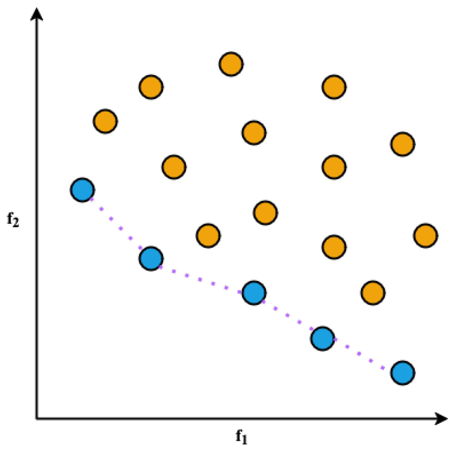
Figure 2.
Illustration of the 4-bit parity problem: given a 4-bit input string, the goal is to return 1/0 when the number of 1-bits is even/odd. It is worth noting that the parity value for a sequence made of 0-bits only is 1.
Figure 2.
Illustration of the 4-bit parity problem: given a 4-bit input string, the goal is to return 1/0 when the number of 1-bits is even/odd. It is worth noting that the parity value for a sequence made of 0-bits only is 1.
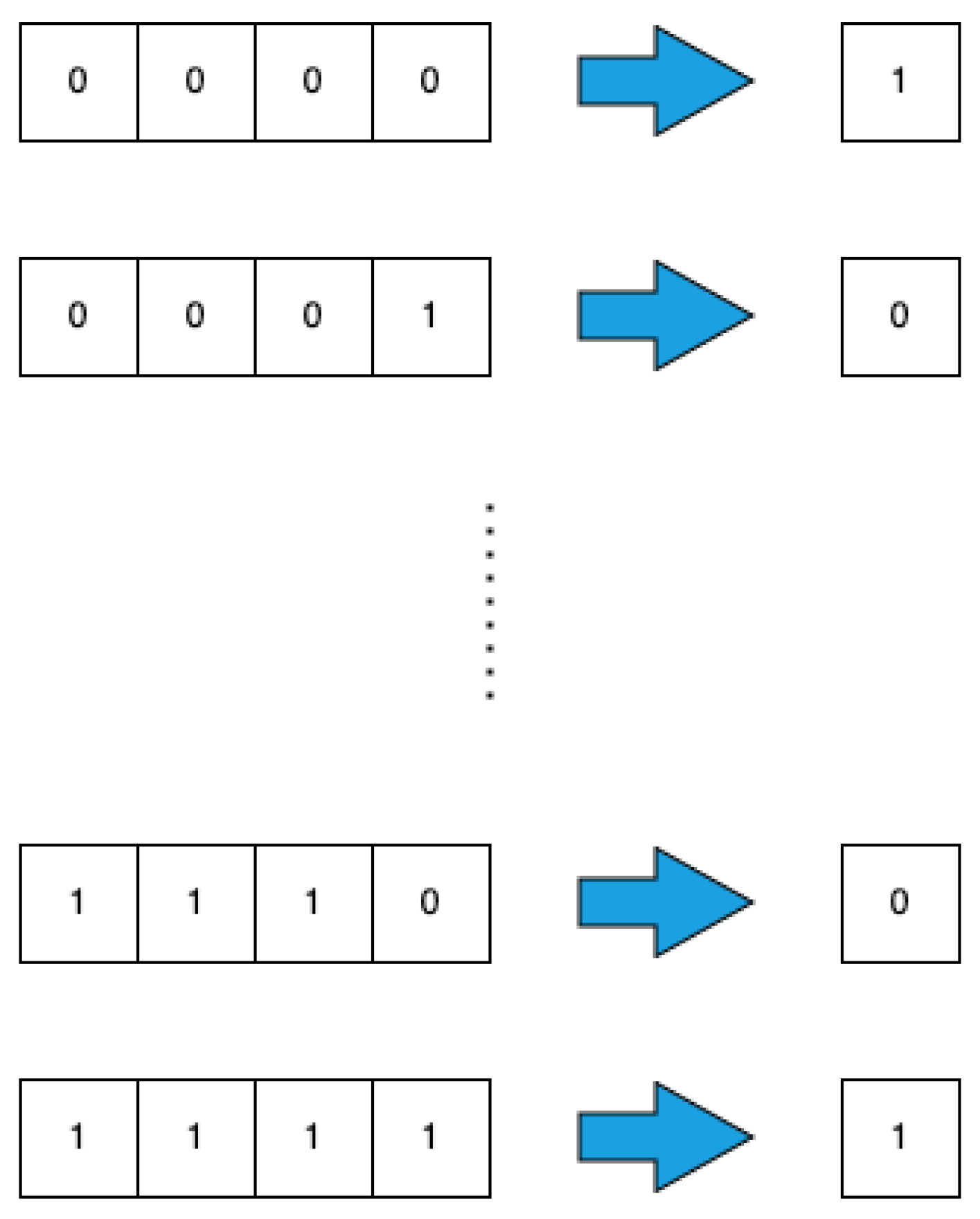
Figure 3.
Double-pole balancing problem: two poles are placed (green rectangles) are placed on the top of wheeled mobile cart (orange rectangle), which can move on a horizontal surface (light blue rectangle).
Figure 3.
Double-pole balancing problem: two poles are placed (green rectangles) are placed on the top of wheeled mobile cart (orange rectangle), which can move on a horizontal surface (light blue rectangle).
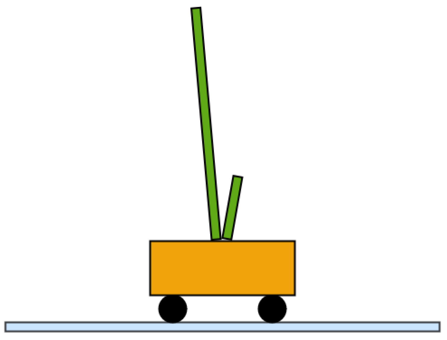
Figure 4.
Grid navigation problem: an agent (red circle) has to navigate in a grid world. The agent starts from one of four possible initial locations (yellow squares) and its goal is to reach the target location (red square). The agent can move left, up, right or bottom.
Figure 4.
Grid navigation problem: an agent (red circle) has to navigate in a grid world. The agent starts from one of four possible initial locations (yellow squares) and its goal is to reach the target location (red square). The agent can move left, up, right or bottom.
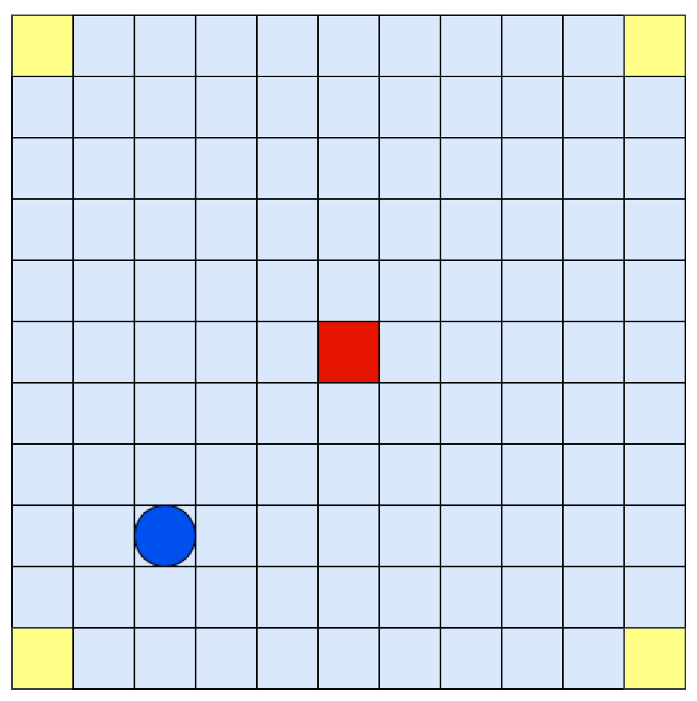
Figure 5.
Schematic of the considered EAs. (a) GGA; (b) OpenAI-ES; (c) SSS; (d) SSSHC.
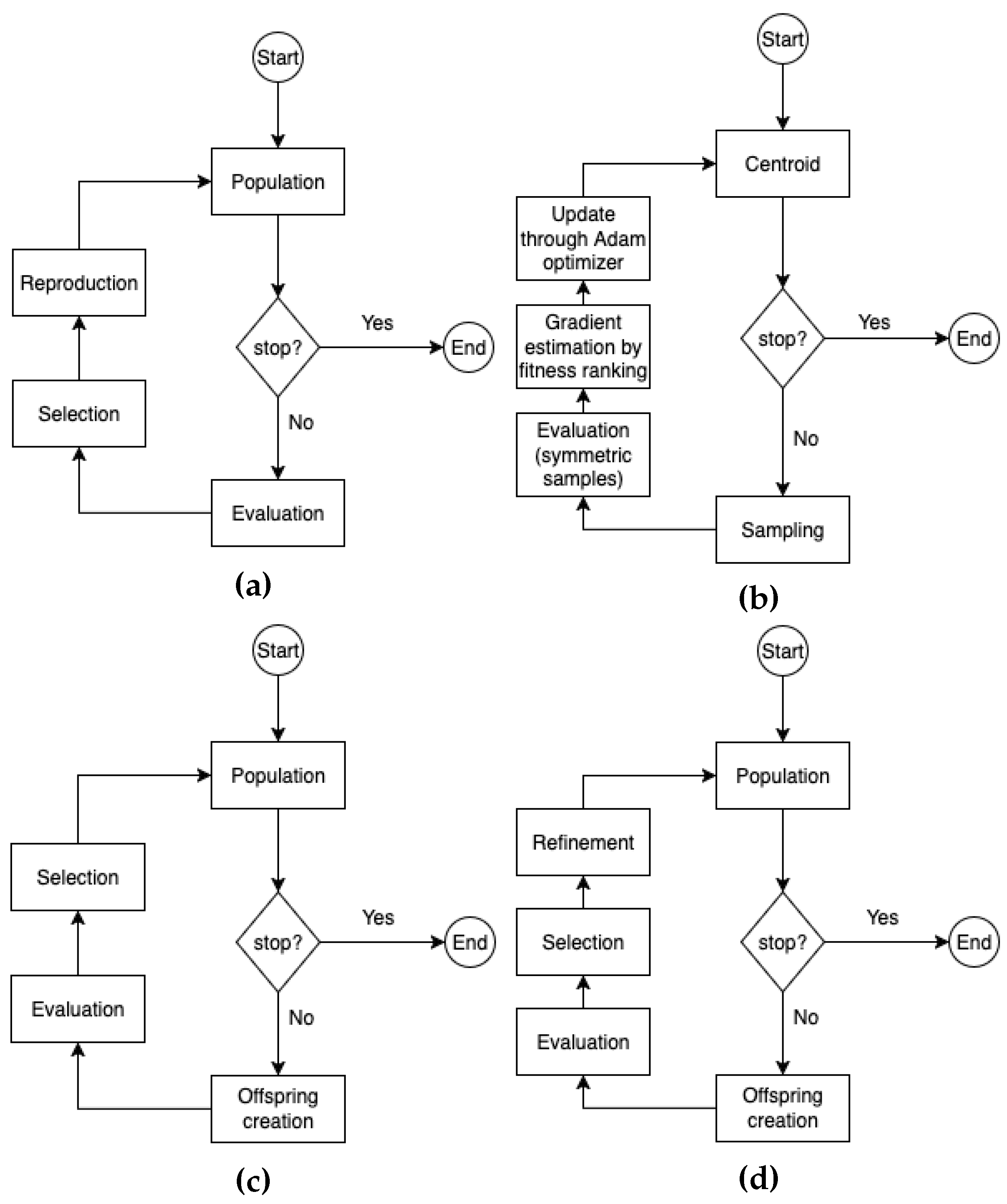
Figure 6.
Performance of GGA, OpenAI-ES, SSS and SSSHC during evolution. The shaded areas are bounded in the range (first and third quartiles of data). We use the logarithmic scale on the y-axis to improve readability. Fitness is averaged over 30 replications.
Figure 6.
Performance of GGA, OpenAI-ES, SSS and SSSHC during evolution. The shaded areas are bounded in the range (first and third quartiles of data). We use the logarithmic scale on the y-axis to improve readability. Fitness is averaged over 30 replications.
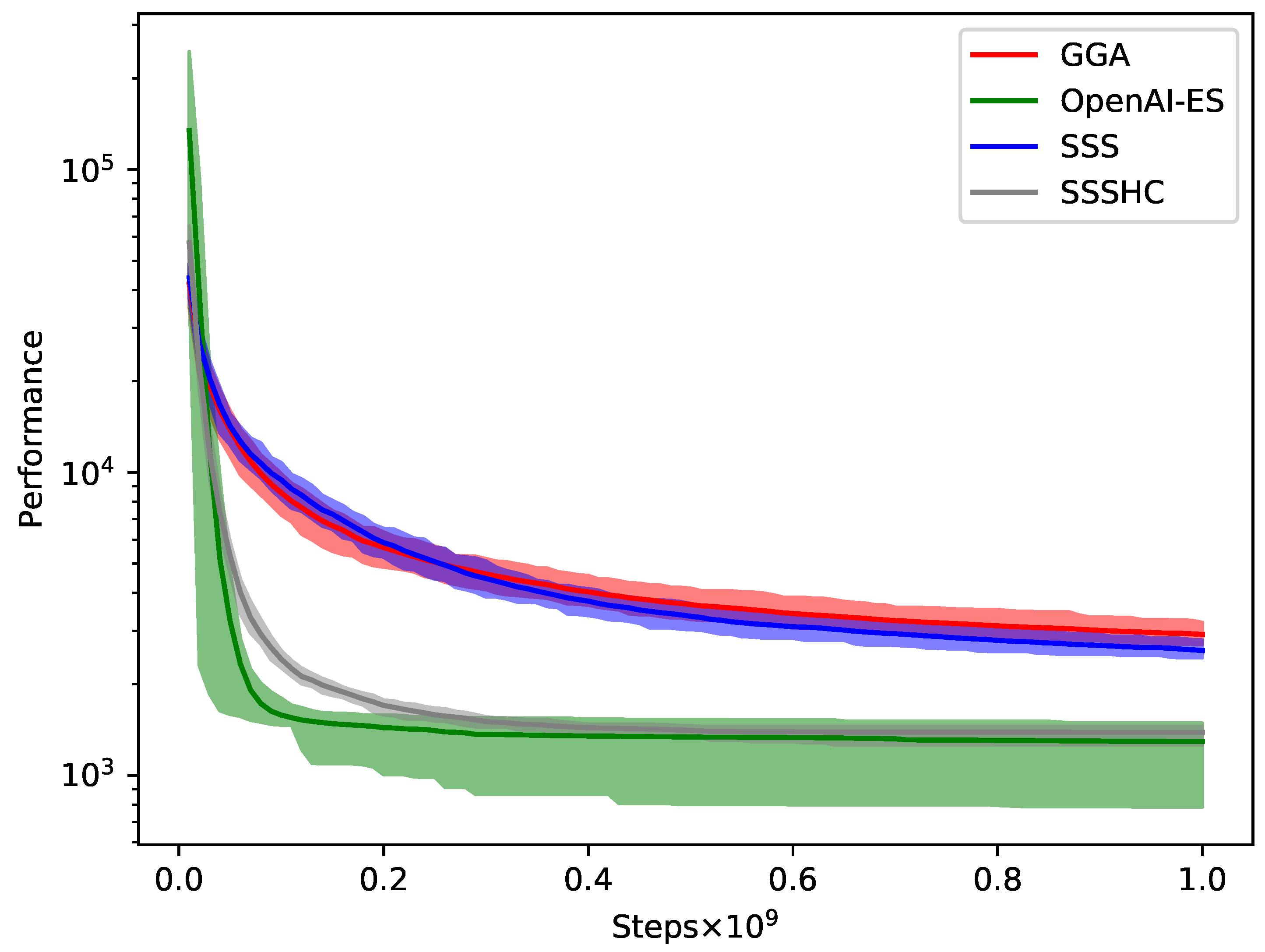
Figure 7.
Final performance achieved by the different methods (see Table 5). Boxes are bounded in the range , with the whiskers extending to data within . Medians are indicated with yellow lines. The notation indicates that the fitness values of the two considered methods do not statistically differ (Mann-Whitney U test with Bonferroni correction, , see also Table 6).
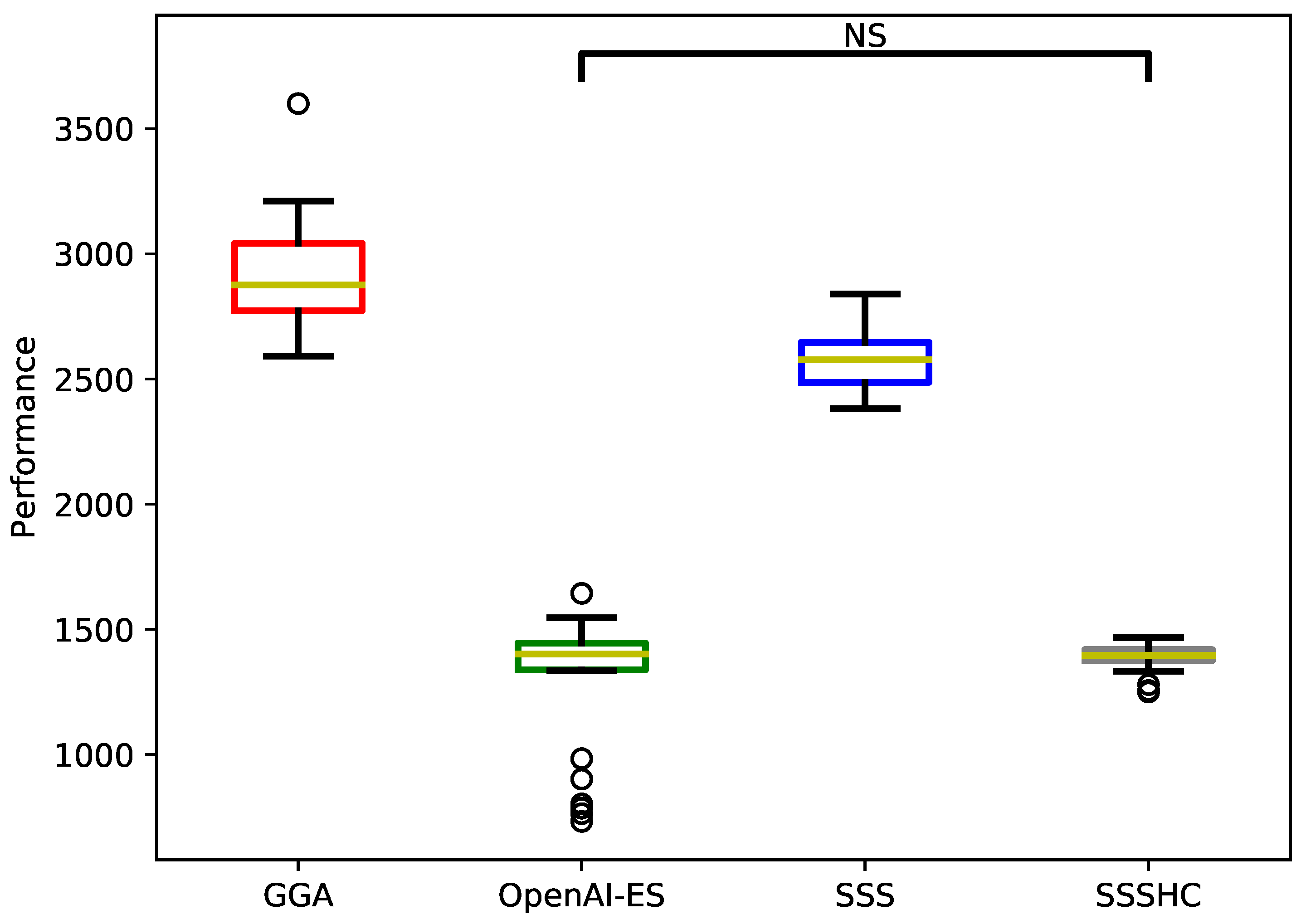
Figure 8.
Analysis of the algorithm performance on the different problems. Black lines mark the standard deviations. We use the logarithmic scale on the y-axis to improve readability. Bars denote the average fitness from 30 replications.
Figure 8.
Analysis of the algorithm performance on the different problems. Black lines mark the standard deviations. We use the logarithmic scale on the y-axis to improve readability. Bars denote the average fitness from 30 replications.
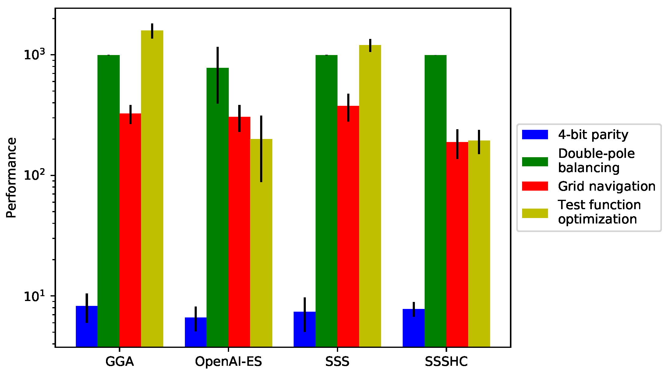
Figure 9.
Algorithm performance on the Ackley, Griewank, Rastrigin, Rosenbrock and Sphere test functions. Boxes are bounded in the range , with the whiskers extending to data within . Medians are indicated with yellow lines. We use the logarithmic scale on the y-axis to improve readability. Data represents the average fitness from 30 replications.
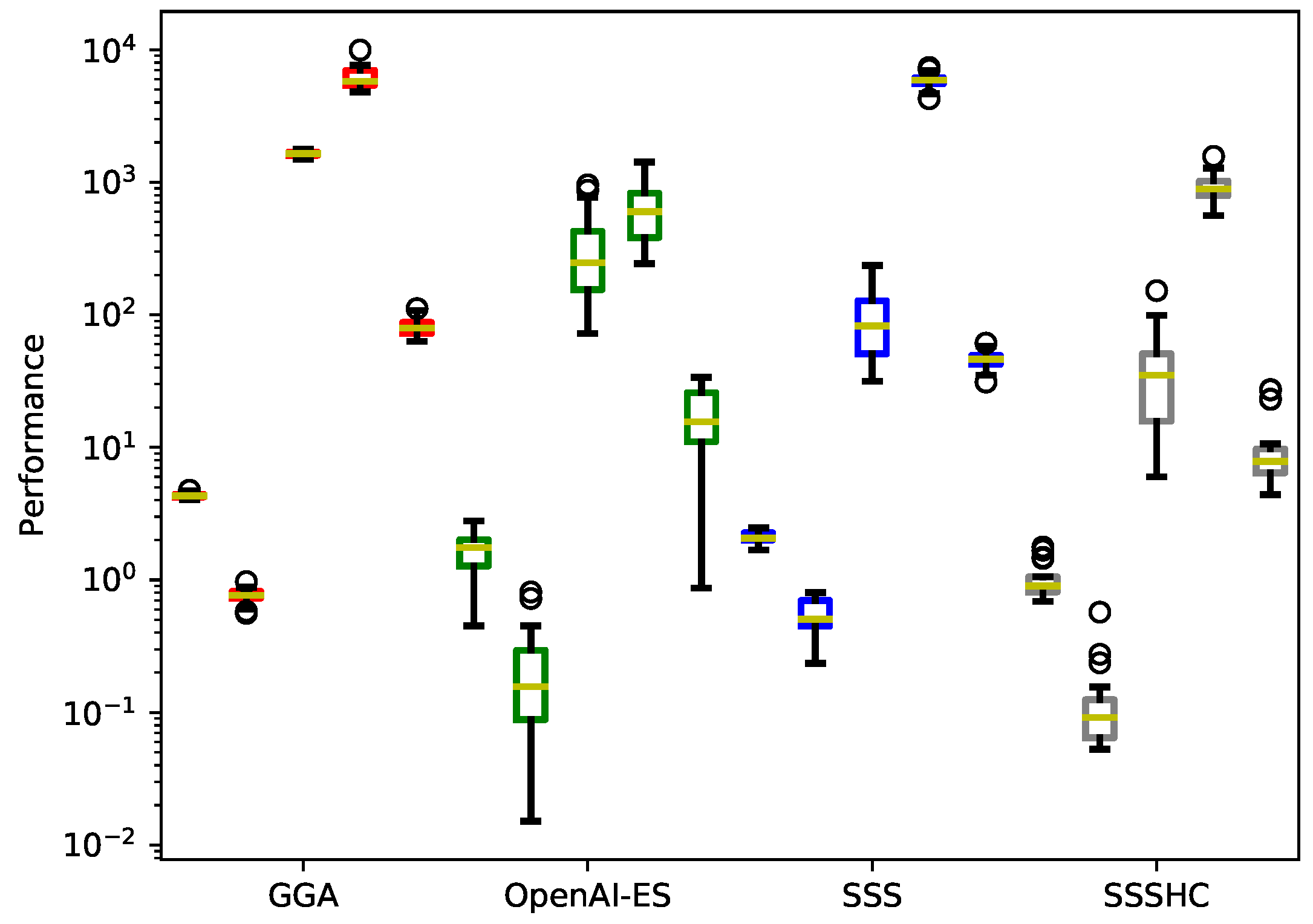

Table 1.
Parameters characterizing the double-pole balancing problem. The track extremes are placed at -2.4 m and 2.4 m, respectively. We denote the absence of information with the symbol “-”.
Table 1.
Parameters characterizing the double-pole balancing problem. The track extremes are placed at -2.4 m and 2.4 m, respectively. We denote the absence of information with the symbol “-”.
| Parameter | Length | Mass |
| Track | 4.8 m | - |
| Cart | - | 1.0 kg |
| Long pole | 1.0 m | 0.5 kg |
| Short pole | 0.1 m | 0.05 kg |
Table 2.
Initialization of the state variables in each trial of the double-pole balancing problem.
| x | ||||||
| 1 | -1.944 | 0 | 0 | 0 | 0 | 0 |
| 2 | 1.944 | 0 | 0 | 0 | 0 | 0 |
| 3 | 0 | -1.215 | 0 | 0 | 0 | 0 |
| 4 | 0 | 1.215 | 0 | 0 | 0 | 0 |
| 5 | 0 | 0 | -0.10472 | 0 | 0 | 0 |
| 6 | 0 | 0 | 0.10472 | 0 | 0 | 0 |
| 7 | 0 | 0 | 0 | -0.135088 | 0 | 0 |
| 8 | 0 | 0 | 0 | 0.135088 | 0 | 0 |
Table 3.
Encoding of the input () and output () neurons used for 4-bit parity, double-pole balancing and grid navigation problems. Symbols are defined as follows: concerning 4-bit parity, (with ) states for the generic bit of the input string, whereas indicates the network output used to check parity. As regards double-pole balancing, x refers to the cart position, and denote the angle of the long and short poles, respectively, and is a flag indicating whether the trial might prematurely be stopped because either the cart is going out of the track () or the pole angles are above , while is the force applied to the cart that determines its motion. Lastly, with respect to grid navigation, the symbols and represent, respectively, the position of the agent and of the target locations, is the grid size and is the direction of the agent in the grid (with ).
| Problem | |||||
| 4-bit parity | |||||
| Double-pole balancing | alert | ||||
| Grid navigation |
Table 4.
List of parameter settings used for the different algorithms. Symbol refers to the number of replications, indicates the number of evaluation steps (i.e., the length of evolution), denotes the number of solutions forming the population. Concerning GGA, and represent, respectively, the number of reproducing solutions (i.e., the ones that have been selected) and the number offspring generated by each selected solution. The symbol is the mutation rate (i.e., the probability to modify one gene), while refers to the probability of performing (asexual) crossover. With respect to OpenAI-ES, denotes the learning rate and is the number of samples extracted from the Gaussian distribution. The symbol indicates the number of refinement iterations performed by SSSHC. Lastly, the symbol refers to the range of connection weights.
| Parameter | GGA | OpenAI-ES | SSS | SSSHC |
| 30 | ||||
| 100 | 1 | 50 | 50 | |
| 10 | - | |||
| - | ||||
| Yes | - | Yes | ||
| - | ||||
| - | - | |||
| - | 20 | - | ||
| - | 5 | |||
Table 5.
Fitness analysis of the different algorithms. Data is the average of 30 replications of the experiments. Best performance is reported in bold.
Table 5.
Fitness analysis of the different algorithms. Data is the average of 30 replications of the experiments. Best performance is reported in bold.
| GGA | OpenAI-ES | SSS | SSSHC |
| 2915.823 [206.120] | 1291.433 [268.231] | 2581.040 [117.146] | 1384.418 [57.312] |
Table 6.
Statistical comparison between the considered methods according to the Mann-Whitney U test with Bonferroni correction, with significant differences indicated in bold. Table is symmetrical with respect to the main diagonal. The symbol “-” marks the absence of the corresponding entry. Data is the average of 30 replications of the experiments.
| GGA | OpenAI-ES | SSS | SSSHC | |
| GGA | - | |||
| OpenAI-ES | - | |||
| SSS | - | |||
| SSSHC | - |
Table 7.
Analysis of the performance collected by the different algorithms with regard to 4-bit parity, double-pole balancing, grid navigation and test function optimization. Bold values correspond to the best outcomes. Data is the average of 30 replications of the experiments.
Table 7.
Analysis of the performance collected by the different algorithms with regard to 4-bit parity, double-pole balancing, grid navigation and test function optimization. Bold values correspond to the best outcomes. Data is the average of 30 replications of the experiments.
| Problem | GGA | OpenAI-ES | SSS | SSSHC |
| 4-bit parity | 8.233 [2.246] | 6.633 [1.538] | 7.367 [2.331] | 7.800 [1.078] |
| Double-pole balancing | 994.654 [2.199] | 778.279 [384.148] | 993.708 [2.394] | 993.725 [1.601] |
| Grid navigation | 325.167 [57.660] | 306.142 [75.842] | 377.092 [97.762] | 188.908 [51.606] |
| Test function optimization | 1587.770 [223.944] | 200.379 [111.980] | 1202.873 [147.151] | 193.986 [43.340] |
Table 8.
Analysis of the performance collected by the different algorithms with regard to the Ackley, Griewank, Rastrigin, Rosenbrock and Sphere test functions. Last row reports the average fitness and the standard deviation. Bold values correspond to the best outcomes. Data is the average of 30 replications of the experiments.
| Test function | GGA | OpenAI-ES | SSS | SSSHC |
| Ackley | 4.331 [0.179] | 1.673 [0.586] | 2.107 [0.184] | 0.994 [0.282] |
| Griewank | 0.765 [0.094] | 0.217 [0.193] | 0.546 [0.146] | 0.120 [0.098] |
| Rastrigin | 1643.956 [66.687] | 332.113 [245.317] | 97.339 [53.305] | 39.996 [32.509] |
| Rosenbrock | 6207.401 [1112.739] | 650.228 [317.946] | 5868.017 [702.571] | 918.511 [209.908] |
| Sphere | 82.393 [12.567] | 17.665 [9.097] | 46.356 [6.654] | 10.307 [6.656] |
| Average | 1587.769 [2444.544] | 200.379 [314.326] | 1202.873 [2354.027] | 193.985 [374.800] |
Table 9.
Analysis of the weight size of the controllers evolved with the different EAs. Data is the average of 30 replications of the experiments.
Table 9.
Analysis of the weight size of the controllers evolved with the different EAs. Data is the average of 30 replications of the experiments.
| GGA | OpenAI-ES | SSS | SSSHC |
| 0.316 [0.047] | 0.083 [0.045] | 0.124 [0.045] | 0.018 [0.015] |
Table 10.
Worst fitness value that can be obtained in each considered problem.
| 4-bit parity | Double-pole balancing | Grid navigation | Test function optimization |
| 16 | 1000 | 500 | 6450690.655 |
Disclaimer/Publisher’s Note: The statements, opinions and data contained in all publications are solely those of the individual author(s) and contributor(s) and not of MDPI and/or the editor(s). MDPI and/or the editor(s) disclaim responsibility for any injury to people or property resulting from any ideas, methods, instructions or products referred to in the content. |
© 2025 by the authors. Licensee MDPI, Basel, Switzerland. This article is an open access article distributed under the terms and conditions of the Creative Commons Attribution (CC BY) license (http://creativecommons.org/licenses/by/4.0/).
Copyright: This open access article is published under a Creative Commons CC BY 4.0 license, which permit the free download, distribution, and reuse, provided that the author and preprint are cited in any reuse.


