
Submitted:
06 November 2023
Posted:
07 November 2023
You are already at the latest version
Abstract
When describing the tribological behaviour of technical surfaces, the need for full length scale microtopographic characterization often arises. The self-affine of surfaces and the characterization of self-affine by a fractal dimension and its implantation into tribological models are commonly used. The goal of our present work was to determine the frequency range of fractal behaviour of surfaces by analysing the microtopographic measurements of a brake plunger. We also wanted to know if the bifractal and multifractal behaviour can be detected in real machine parts. As a result, we developed a new methodology for determining the fractal range boundaries to separate the nano- and micro-roughness. In order to reach our goals, we used atomic force microscope (AFM) and stylus instrument to provide measurements in wide frequency range (19 nm - 3 mm). As a result of the power spectral density (PSD) based fractal evaluation, it was found that the examined surface could not be characterized by a single fractal dimension and that we developed a methodology for stopping the margin of validity of each fractal dimension, and we also developed a methodology for determining the limits of validity of certain fractal dimensions.
Keywords:
roughness
; fractal
; bifractal
; full length scale
; microtopograpy
; nanoroughness
; power spectral density
1. Introduction
To characterize surface microgeometry, separation of roughness and waviness has been included for decades. Separation of unequal components of different wavelengths from different sources carries important information on the formation of each microgeometric element. They also play a different role in tribological processes, so the identification of each wavelength component is an important element in understanding friction, wear and lubrication phenomena.
Different components of surface unevenness have different sources. The waviness of the surface bear a relation to operating parameters of production process, such as the vibration of cutting machine. The microroughness is influenced by tools and production parameters of surface finishing process, such as cutting tool geometry or cutting parameters. Submicro/nano roughness is related to the material composition and microstructure of materials for instance in case of coatings.
Surface unevenness is one of the parameters are influence the contact behavior of tribological processes. Different order of surface roughness—depending on the hardness of the contacting materials—has different effect to real contact area [1] and wear resistance [2]. [3] overview many tribological phenomena where surface nano- or micro roughness has significant effect, and authors overview the measuring technics and their limitations in frequency range. But use different measuring techniques is not enough to separate micro and nano roughness.
In roughness measurements, RC and Gauss filters have traditionally been used to separate roughness and waviness. To meet growing demands, the enhanced dual-Gauss filter, the robust or the spline filters are available for industry and researchers [4,5,6]. The evaluation technique based on motif combinations, where there are also ways of separating roughness and waviness, has had long traditions [7]. The German automotive standard introduced the so-called dominant wavelength concept [8] in the early 2000s, but morphological screening methods have also been revived [9,10]. Besides, full frequency spectrum tests have had an increasing role [8,10,11], which are no longer intended to identify the frequencies but to characterize the surfaces in the frequency space. These include wavelet-based characteristics, correlation functions, and amplitude density spectra based on Fourier transform [13,014,15]. The most important advantage of these methods is that, while conventional convolutional filters seek to separate the large and small spaced elements by providing cut-off and weight functions, the PSD (Power Spectral Density) analysis (and partly other methods) performs a true frequency separation.
The special evaluation of PSD analysis is suitable for fractal characterization of surfaces [9]. The fractal dimension is a feature of self-affine. In case of technical surfaces self-affine in nature is proven [14,15], but the determination of fractal dimension of surfaces and especially the use of fractal characterization have many contradictions [17,18]. At present, there is no unified standpoint and methodology that would accept the use of fractal technology to characterize technical surfaces, although many tribological method—friction and hysteresis loss calculation theory [9,11,19,20,21]—builds on the fractal nature of surfaces and requires a full spectrum analysis which the classical roughness parameters are unable to provide due to the relatively narrow frequency range of measurements.
The use of PSD analysis and fractal evaluation often leads to controversial results, so its use to characterize technical surfaces requires caution. Our earlier studies [22] revealed the limitations of PSD-based evaluation techniques in which the sampling step of the roughness measurement, the frequency step of the PSD curve, and the method of determining the Hurst exponent were included as critical points. In our further investigations [23], we successfully applied the methodology to characterize surfaces of different tribological behavior, where the use of standard roughness parameters was not successful but fractal-based evaluation proved to be useful in surface characterization.
However, the most important question of the self-affine of surfaces seems to be whether this self-affine really means a full spectrum analysis. That is, can the examination of a frequency range (which is practically limited by the sampling distance of the measurement performed from the bottom and the measurement length from the top) be extended to the full spectrum, assuming that this self-affine is the same at all frequency levels? Bhushan’s examinations treated surfaces as bifractals as early as 1992 [24], but only the frequency range below and above the dominant wavelengths was separated. In recent years, however, several authors—such as Wu [18], Le Gal [11], Ţălua [25]—apply the terms bi- and multifractal, but in each case, they interpret concepts in a wavelength range smaller than the dominant wavelength. However, methodologically it is not clear how we can limit the beginning and end of each fractal nature.
In recent studies [26,27,29] the correlation of bifractal behavior and tribological (contact or wear) properties are examined. Scientists use the term of bifractal and define two fractal dimensions, although the separation of the regimes is not exact.
The objective of our research was, on the one hand, to find whether the bifractal and multifractal behaviour can be detected in real machine parts. On the other hand, we tried to find the methodology for determining the fractal range boundaries to separate micro- and nano-roughness.
The separation—based on a physical content of surface roughness—provide an opportunity to distinguish the sources of nano- and microroughness and helps the material scientist and product engineers to choose and to design the operationally optimized surface structure also in nano- and in micro-range.
2. Materials and Methods
2.1. Measurements of brake plunger
Brake system is one of the most essential elements of automobiles. Typical the force applied on brake pedals is converted into hydraulic pressure in the master cylinder, which consists of two plungers. Plungers operate separately. The brake plunger is in its initial position when the pedal is released and moves forward during the braking process. The primary plunger is operated through the brake pedal while the hydraulic pressure between the primary and secondary plunger forces the secondary plunger to compress the fluid in its circuit. During the motion of the plungers the plunger/rubber seals contact results friction force. This friction loss causes that the hydraulic pressure is different in the two separate brake circuits. Therefore it is important to be the friction force at the plunger/rubber seal contact as minimal as possible. Former investigations [23] proved that the surface roughness of the plunger plays a considerable role on the friction force. The scheme of profile and topographic measurements positions and a photo of the measured plunger can be seen in Figure 1.
To examine the surface roughness of brake plunger two type of measuring system were used. The goal was to provide the wide frequency scale investigations. Different measuring equipment a Mahr Perthometer Concept stylus instrument and D3100 atomic force microscope were used.
The stylus instrument of Bánki Donát Faculty of Mechanical and Safety Engineering, Óbuda University had an FRW750 diamond cone stylus of 5 μm peak radius and 90° peak angle which provided the higher wavelength scale measurements. The atomic force microscope (AFM) of Chemical Research Centre of Hungarian Academy of Sciences with IIIA controller and Dimension 1951e type scanner was used to carry out the low wavelength scale measurements.
In the course of the investigations, measurements were performed with 2 primary plungers of the same technology (indicated with A and B). The first part of the tests aimed to determine the dominant wavelength of the surface. For this purpose, standard roughness measurements were performed on a Mahr Perthometer Concept stylus roughness measuring instrument on a measuring length of 5.6 mm, with 10 roughness profiles, parallel to the length of the part, on both specimens. Measurements were made in accordance with ISO 4287 standards. This was followed by topographic measurements, for which the measurement settings are summarized in Table 1. Sampling distances were the same in booth x and y directions.
2.2. Characterisation techniques
We used several methods to evaluate the measurements in order to obtain reliable results.
To determine the dominant wavelength of the surface, the parameter RSm (mean distance of profile elements) was used, which is defined in ISO 4288. In addition, on the roughness profiles, power spectral density analysis was performed to identify the dominant wavelength. The methodology used was described in our earlier work [23]. The following example of a turned profile (see Figure 2a) produced with feed rate of 50 µm/revolution illustrates the application of the method. The tool marks have periodical character, but they differ from the common turning grooves. There are two possibilities of showing results. One is to represent the amplitude of PSD in the function of wavelength (see Figure 2b). The practical gain of the first representation is that dominant wavelength components appear as peak point of the PSD curve. Despite the unusual form of tool marks the highest point of the PSD curve can be found at 50 µm, indicating that this is the dominant wavelength of the profile.
The other prevalent method (that is the base of our fractal analysis) is the logarithmic scale frequency-PSD amplitude visualization (see Figure 2c). As it can be seen the high frequency range of the curve can be approximated by a straight line. The slope of the line is in correlation with the fractal dimension of the profile. In this case, wavelengths smaller than 1/q* play a considerable role.
By identifying the dominant topographic elements, slicing technique was used (see methodology on Figure 3 and details in [28]).
Ratio of the small and large axis of the roughness peaks was determined. The slicing technique was applied to the largest measured topography (3 mm × 3 mm). The slicing height showing the highest number of roughness peaks was 0.803 μm, where 135 peaks were identified. At this level, the size of the roughness peaks was interpreted by defining the ratio of the large and small axes of roughness peaks, the measured surface was covered with 135 equal rectangles (according to the ratio of large and small axes obtained), to determine the average size of the dominant elements.
To determine the fractal dimension, 3D topographic measurements were used. For the evaluation, 3D PSD analysis was performed. Figure 4. represents the basic steps of the applied method and mathematical details can be found in [23].
In 3D PSD analysis the frequency range depends on the measured area and sampling distance. The lowest frequency was the reciprocal of the measuring length while the upper limit has based on the Nyquist-Shannon sampling theorem. This frequency range was divided into 125 parts in both coordinate directions and then, by means of a consolidation proposed by Persson [9], a 2D logarithmic scale PSD curve was formed. The base of the Persson’s reduction is that PSD topography seems like a truncated cone that needs only two coordinates (namely the height and the radius) to be described. The resulting 15625-point PSD curve was used to determine the slope of the curve from which the fractal dimension can be determined.
The final step of the studies was the interpretation of fractal dimension values in a frequency spectrum. Since the measurements covered different frequency spectra, it was possible to assign the fractal dimensions defined in the different frequency ranges to the frequency band. In practice, this meant that the value of the fractal dimension of the given measurement was assigned to the mean value of the frequency range of each measurement and the resulting points were plotted on a logarithmic frequency scale. No similar methodology was found in the literature.
3. Results
3.1. Dominant wavelength
The wavelength of measurements on roughness profiles is indicated by the parameter of average distance of the profile elements (RSm). The average RSm parameter on the 10 measured profiles was 163.1 μm with a deviation of 24.6 μm. A typical roughness profile of the surface is shown in Figure 5. The PSD function of the profiles is much more informative. Figure 6 shows the PSD amplitude dependent on the wavelength, of which the 178 μm value stands out indicating the dominant wavelength of the surface.
The stylus microtopography of the surface can be seen in Figure 7 and Figure 8. Figure 7 shows the surface area of 1 mm x 1 mm, while Figure 8 shows a 200 μm × 200 μm portion of this. Determining the dominant wavelength is not easy either here—as it can be seen in the profile of Figure 5—the dominant elements on the surface have 2-4 local maxima. Note that the value of RS parameter—average distance of local maxima—was 32.9 μm on average measured profiles, i.e., significantly different from RSm. This effect can be detected in the PSD curve and the topographic image, too.
When applying the slicing technique, the interrelated set of points above the slicing planes are interpreted as roughness peaks, regardless of whether they have one or more local maximum. Thus, it is possible that this technique identified 135 peaks at the topography of 3 mm × 3 mm at a height of 0.803 μm (slicing below this level the number of identified peaks decreased as more and more surface areas were merged while above this level also decreased because we have cut in less and less material, that is, we only identified the “peak” peaks). Figure 9 shows the distribution function of the ratio of the major axis connecting the outermost points of the identified roughness peaks and the perpendicular minor axis. The maximum of the curve is 1.7, which means slightly extended peaks. If the measuring area is covered with 135 rectangles of 1.7 side ratio, the rectangles have side lengths of 95 and 161 μm.
The dominant wavelengths that can be determined by the three techniques are 160-180 μm, but due to the fragmentation of the surface, smaller (35-40 μm) and larger (220 μm) dominant elements also occur.
It is important to note that the applied sampling step remains significantly below the dominant wavelength of the surface even in the case of the rarest scan (3 mm × 3 mm topography). This is a necessary condition for reliable fractal evaluation. It is also important to point out that the measurement range of AFM measurements (5 μm to 90 μm) is below the dominant wavelength, i.e., focuses on some details of dominant microtopographic elements. Although the dominant topographic elements or comparable but smaller counterparts are still recognizable on AFM measurement of 90 × 90 μm2 measuring area shown in Figure 10.
3.2. Fractal analysis
During the fractal analysis of the surfaces, the breakpoint typical of the dominant wavelength, already mentioned by Bhushan, was still identifiable on the larger frequency ranges (3 × 3 and 1 × 1 mm2 surfaces). Figure 11a shows the 3 × 3 mm2 topography of PSD topography, while the PSD topography proposed by Persson is merged into the 2D PSD curve in Figure 11b. Black curve represents the smoothing of 200 linear moving average of the PSD curve. The end of the horizontal initial section is unclear, but the peak at λ0 gives the dominant wavelength at 155 μm; it correlates well with previous results of profile analysis (163, 178 and 161 μm). In the highlighted blue part of Figure 11b the linear regression line can be seen. The fractal dimension in the given frequency range was determined from the slope of this straight line.
In case of AFM measurements, where the lowest frequencies obtained from the measurements are below the dominant frequency of the surface, the horizontal initial phase of the PSD curves is missing. This can be seen in Figure 12., which shows the analysis of the 25 μm × 25 μm surface area.
The results of the fractal dimension are summarized in Table 2.
4. Discussion
The final step of the studies was the interpretation of fractal dimension values in a frequency spectrum (represented by sampling distance). The results (see Table 2) of the examinations were presented in a novel approach shown in Figure 13. We did not just move from a space range to a frequency range (realized by PSD analysis) but we created a frequency domain-fractal dimension link. This meant that the fractal dimension values for each frequency range were displayed.
The effect of inaccuracies caused by different measurement settings cannot be detected in the results due to the small value of the sampling step applied. Thus, the different sampling steps did not cause significant errors in the evaluation. This is supported by the same fractal results of the measurements carried out on the various specimens (see Figure 13 purple points, blue x). The effect of the measurement methodology did not influence the results as well, because although the fractal results were significantly different in the two measurement techniques, the transition can also be observed in the largest increment of AFM measurements. In addition, there is a negligibility of the effect of the sampling step in the case of stylus measurements as all three measurements have the same result. After that we can state that the above method can display the limit point that represents the extreme value of fractality associated with machining. For our investigations, this transition is within the sampling distance of 196.1–1000 nm. This means that the fractal dimension Df = 2.22 for machining is only valid in the frequency range greater than 1 μm. Its upper limit is indicated by the fracture of the PSD curve with dominant wavelengths (155 μm). Under 196.1 nm the fractal dimension is around 2.5. It supposes different sources of surface unevenness in this regime than machining, and it also means that any changes in the production process will not influence this nano-roughness.
This way we can interpret bifractal and multi-fractal terms and with the use of the sampling length (logarithmic scale)—fractal dimension diagram we can determine the wavelengths and the range of interpretations for each fractal dimension.
The fact that the former self-affine disappears below this range can be justified by the topographic image of the smallest AFM measurement surface. The topography shown in Figure 14 is no longer similar to the previous surface structure, its topographical features are not primarily due to the traces of the machining process, but also to the topographical elements that are related to the material structure or other nano-scale characteristics.
5. Conclusions
Concerning the investigations, the following conclusions can be drawn:
The dominant wavelength in the examined surface is in the range of 160-180 μm, which can be supported by multiple evaluation techniques.
Because of the uneven texture of the surface, smaller (35-40 μm) and larger (220 μm) wavelength elements can be found on the surface.
For technical surfaces, the fractal dimension cannot be used for full spectrum analysis. The examined surfaces showed bifractal properties where the Df = 2.22 fractal dimension for machining can only be interpreted in the range of 1 μm - 160 μm. This result confirms the observations of [11], [18] and [25], and limits the applicability of full-length scale tribological models such as in literature [9], [19], [20] and [21].
Logarithmic sampling distance—fractal dimension diagram is suitable for determining bifractal wavelengths. This new approach provides a tool for the separation of nano- and microroughness. Based on this method further investigations can be carried out to find the sources (material structure, production parameters) of different roughness components. Surface engineers can design the micro- and nano-roughness to influence the tribological processes and to optimise the surface for operation.
Author Contributions
Conceptualization; methodology, software, validation, formal analysis, investigation: Árpád Czifra; writing—original draft preparation, writing—review and editing, visualization, supervision: Erzsébet Ancza. All authors have read and agreed to the published version of the manuscript.
Funding
This research received no external funding.
Conflicts of Interest
The authors declare no conflict of interest.
References
- Borodich, F. M., Brousseau, E., Clarke, A., Pepelyshev, A., Sánchez-López, J. C. Roughness of Deposited Carbon-Based Coatings and Its Statistical Characteristics at Nano and Microscales. Frontiers in Mechanical Engineering 2019 Volume 5, Article 14. [CrossRef]
- Terres, M. A., Ammari, L., Chérif, A. Study of the Effect of Gas Nitriding Time on Microstructure and Wear Resistance of 42CrMo4 Steel. Materials Sciences and Applications 2017, Volume 8, No. 6. [CrossRef]
- Gong, Y, Xu, J., Buchanan, R. C. Surface roughness: A review of its measurement at micro-/nano-scale, Physical Sciences Reviews 2018, Volume 3, Article 20170057. [CrossRef]
- Seewig, J. Linear and robust gaussian regression filters. Journal of Physics: Conference Series 2005, Volume 13, pp. 254-257. [CrossRef]
- Krystek, M. Discrete linear profile filters. Tagungsband X. International Colloquium on Surfaces, Chemnitz, Germany, 31. Januar-2. Februar 2000; p. 145-152.
- Svalina, I., Sara Havrlišan, S., Šimunović, K., Šarić, T. Investigation of Correlation between Image Features of Machined Surface and Surface Roughness. Technical Gazette 2020, Volume 27, pp 27-36. [CrossRef]
- Blateyron, F. New 3D Parameters and Filtration Techniques for Surface Metrology. Quality Magazine 2006, Volume 3, pp. 1.-7.
- VDA 2007. Oberflächenbeschaffenheit Definitionen und Kenngrößen der dominanten Welligkeit, 2006.
- Persson, B. N. J., Albohr, O., Trataglino, U., Volokitin, A. I., Tosatti, E. On the nature of surface roughness with application to contact mechanics, sealing, rubber friction and adhesion. Journal of Physics: Condensed Matter 2005, Volume 17, R1-R62. [CrossRef]
- Štrabac, B., Mikó, B., Rodić, D., Nagy, J., Hadžistević, M. Analysis of Characteristics of Non-Commercial Software Systems for Assessing Flatness Error by Means of Minimum Zone Method. Technical Gazette 2020, Volume 27, pp 535-541. [CrossRef]
- Le Gal, A., Guy, L., Orange, G., Bomal, Y., Klüppel, M. Modelling of sliding friction for carbon black and silica filled elastomers on road tracks. Wear 2008, Volume 264, pp. 606-615. [CrossRef]
- Krolczyk G.M., Maruda R.W., Nieslony P., Wieczorowski M. Surface morphology analysis of Duplex Stainless Steel (DSS) in Clean Production using the Power Spectral Density. Measurement 2016, Volume 94, pp. 464–470. [CrossRef]
- Grzesik W., Brol S. Wavelet and fractal approach to surface roughness characterization after finish turning of different workpiece materials. Journal of Materials Processing Technology 2009, Volume 209, pp. 2522–2531. [CrossRef]
- Leach R. Characterisation of Areal Surface Texture, Springer-Verlag: Heidelberg, Germany 2013. [CrossRef]
- Scaraggi M., Angerhausen J., Dorogin L., Murrenhoff H., Persson B.N.J. Influence of anisotropic surface roughness on lubricated rubber friction: Extended theory and an application to hydraulic seals. Wear 2018, Volume 410-411, pp. 43-62. [CrossRef]
- Mandelbrot B. B. The fractal geometry of nature. Henry Holt and Company: New York, United States, 1983. [CrossRef]
- Han J.H., Ping S., Shengsun H. Fractal characterization and simulation of surface profiles of copper electrodes and aluminum sheets. Materials Science and Engineering 2005, Volume 403, pp. 174–181. [CrossRef]
- Wu, J., J. Structure function and spectral density of fractal profiles. Chaos, solitons and fractals 2001, Volume 12, pp. 2481-2492. [CrossRef]
- Hiro Tanaka, Kenta Okui, Yuki Oku, Hironori Takezawa, Yoji Shibutani. Corrected power spectral density of the surface roughness of tire rubber sliding on abrasive material, Tribology International 2021, Volume 153, 106632. [CrossRef]
- Kanafi M. M., Tuononen A. J. Top topography surface roughness power spectrum for pavement friction evaluation. Tribology International 2017, Volume 107, pp. 240–249. [CrossRef]
- Kai Jiang, Zhifeng Liu, Yang Tian, Tao Zhang, Congbin Yang. An estimation method of fractal parameters on rough surfaces based on the exact spectral moment using artificial neural network, Chaos, Solitons & Fractals 2022, Volume 161, 112366. [CrossRef]
- Czifra Á. Sensitivity of power spectral density (PSD) analysis for measuring conditions. Studies in Computational Intelligence 2009, Volume 43, pp. 505-517. [CrossRef]
- Czifra Á., Goda T., Garbayo E. (2011). Surface characterisation by parameter-based technique, slicing method and PSD analysis. Measurement 2011, Volume 44, pp. 906-916. [CrossRef]
- Bhushan B., Majumdar A. (1992). Elastic-plastic contact model for bifractal surfaces. Wear 1992, Volume 153, pp. 53-64. [CrossRef]
- Ţălua S., Bramowiczb M., Kuleszac S., Solaymanid S. Topographic characterization of thin film field-effect transistors of 2,6-diphenyl anthracene (DPA) by fractal and AFM analysis. Materials Science in Semiconductor Processing 2018, Volume 79, pp. 144–152. [CrossRef]
- Borri, C., Paggi, M. Topology simulation and contact mechanics of bifractal rough surfaces. Proceedings of the Institution of Mechanical Engineers, Part J: Journal of Engineering Tribology 2016, Volume 230, pp 1345-1358. [CrossRef]
- Wei, C., Zhu, H., Lang, S. The Bifractal Stratified Characterisation of a Plateau Honing Cylinder Liner Surface Profile During the Wear Process. Fractals 2021, Volume 29, No. 05. [CrossRef]
- Czifra Á., Váradi K., Horváth S. Three dimensional asperity analysis of worn surfaces. Meccanica 2008, Volume 43, pp. 601-609. [CrossRef]
- Vencl, A., Stojanović, B., Gojković, R., Klančnik, S., Czifra, Á., Jakimovska, K., Harničárová, M. Enhancing of ZA-27 alloy wear characteristics by addition of small amount of SiC nanoparticles and its optimisation applying Taguchi method. Tribology and Materials 2022, Volume 1, pp. 96-105. [CrossRef]
Figure 1.
Scheme of measurements and photo of measured primary plunger.
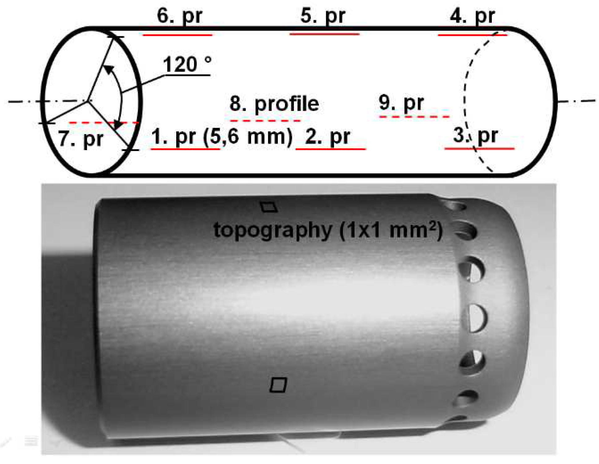
Figure 2.
Turned profile (a) (feed rate is 50 µm/rev.) and PSD curve of the turned profile (b) wavelength dependent representation; (c) frequency dependent representation.
Figure 2.
Turned profile (a) (feed rate is 50 µm/rev.) and PSD curve of the turned profile (b) wavelength dependent representation; (c) frequency dependent representation.
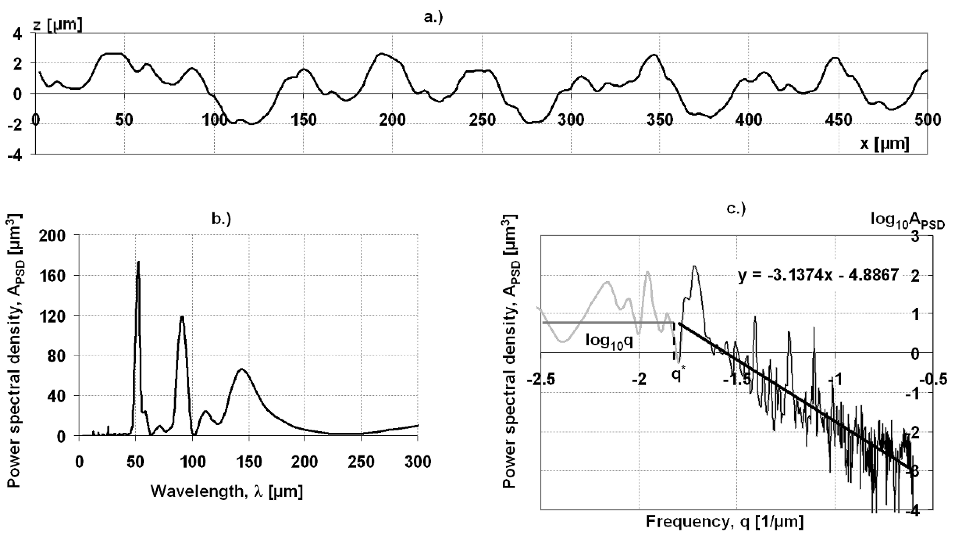
Figure 3.
Asperity detection in the slicing technique.
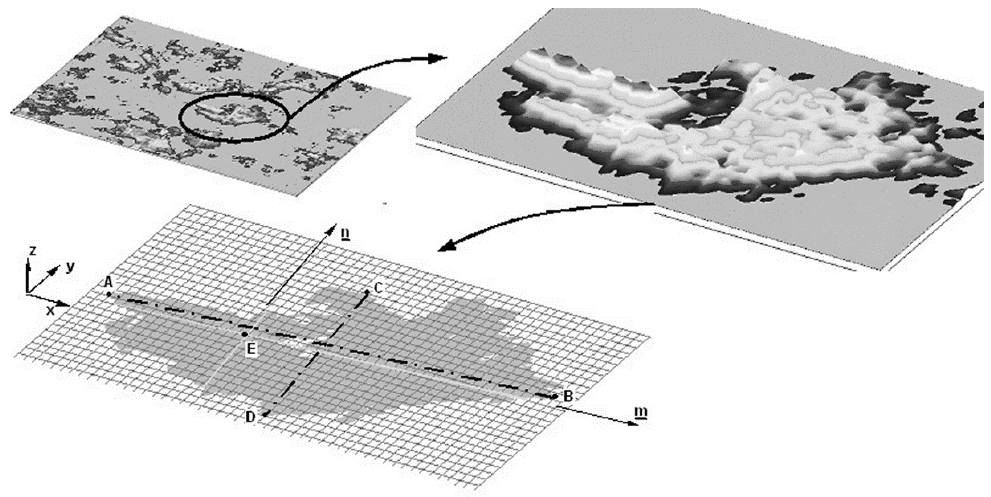
Figure 4.
Method of fractal calculation from topography.
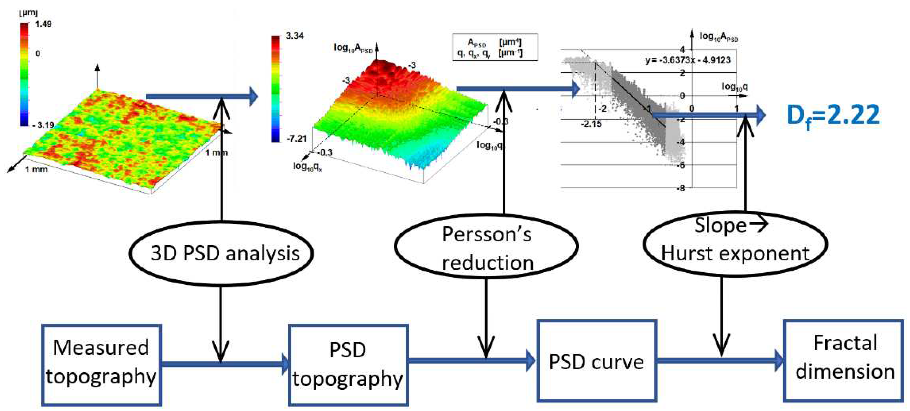
Figure 5.
Roughness profile of measured plunger.
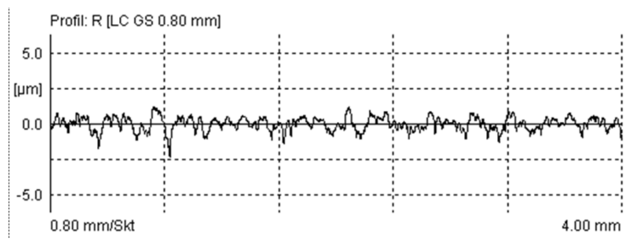
Figure 6.
Power spectral density of measured profiles (λ—wavelength; A(λ)—Amplitude of PSD).
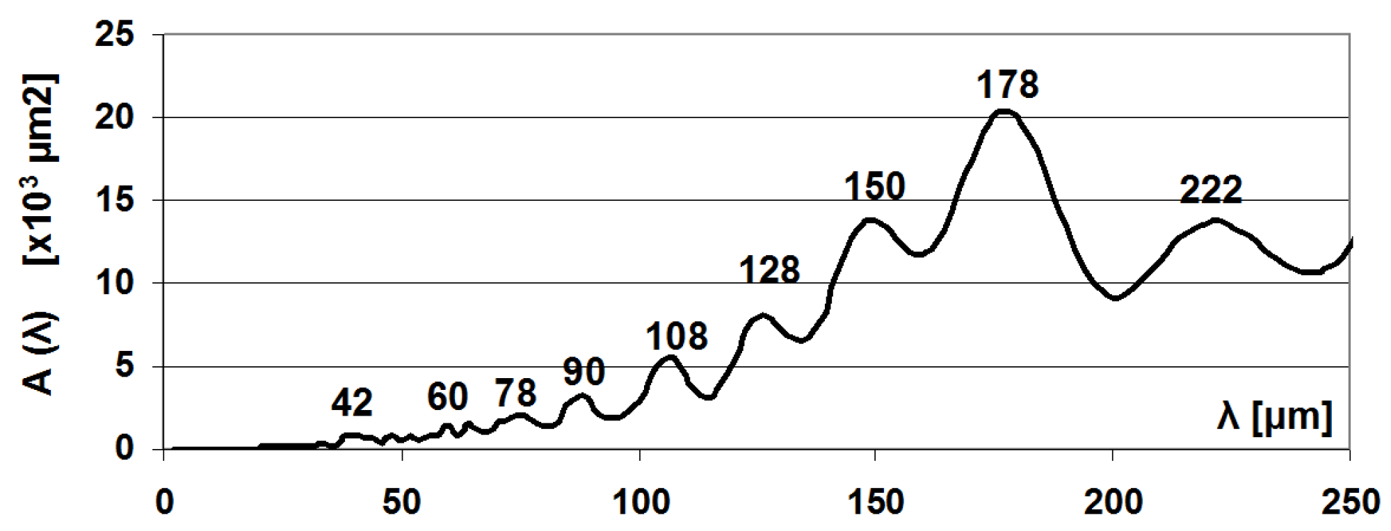
Figure 7.
Measured topography of the plunger; stylus measurement (1 mm by 1 mm measuring area, 1μm by 1 μm sampling).
Figure 7.
Measured topography of the plunger; stylus measurement (1 mm by 1 mm measuring area, 1μm by 1 μm sampling).
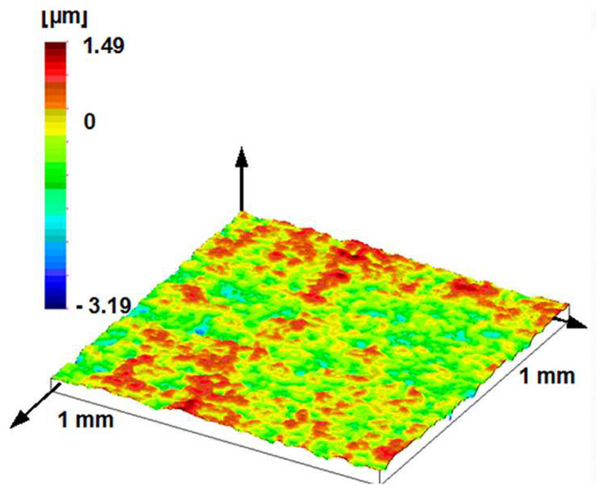
Figure 8.
200 μm by 200 μm part of measured topography of the plunger; stylus measurement (1 mm by 1 mm measuring area, 1μm by 1 μm sampling).
Figure 8.
200 μm by 200 μm part of measured topography of the plunger; stylus measurement (1 mm by 1 mm measuring area, 1μm by 1 μm sampling).
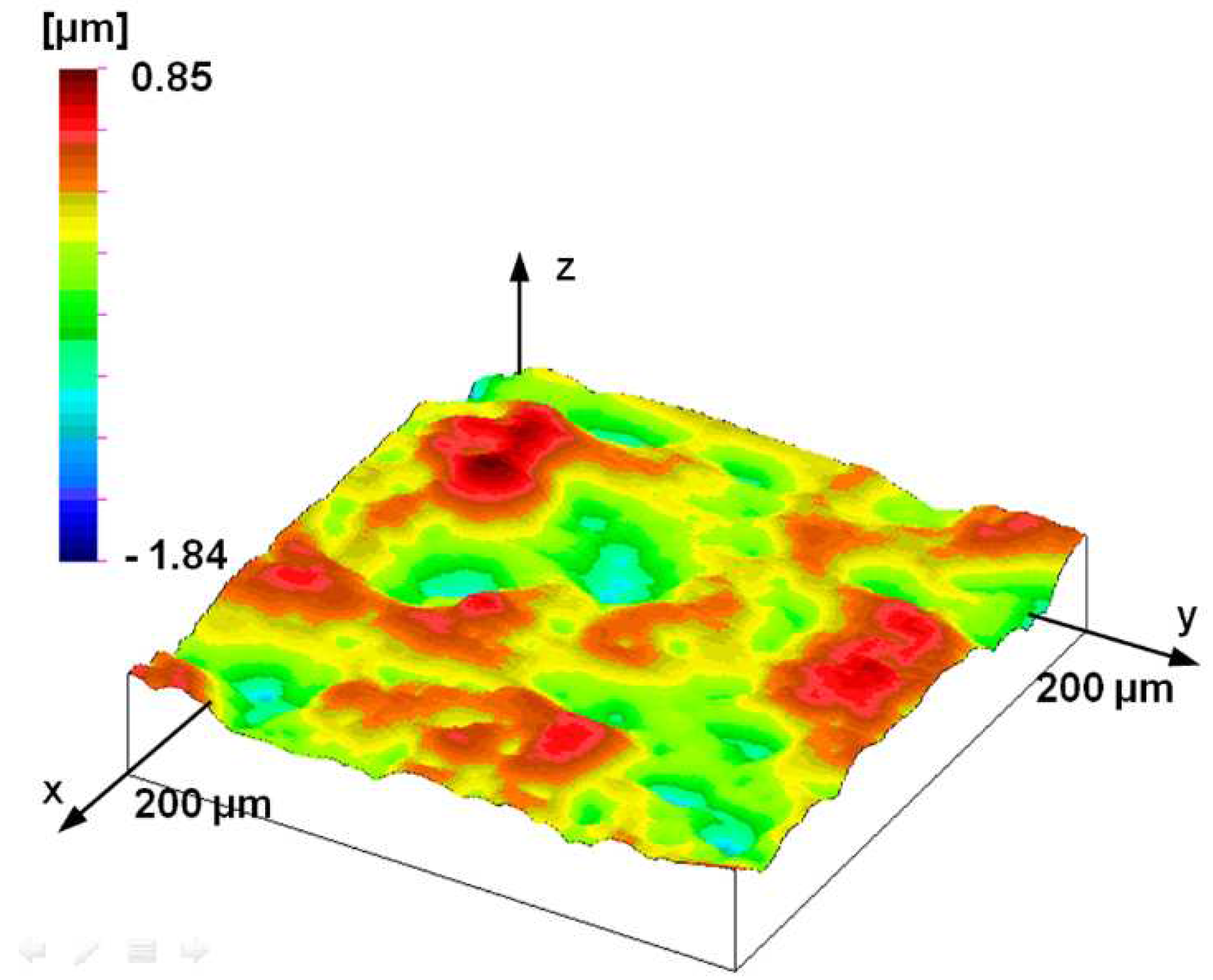
Figure 9.
Distribution of asperity major and minor axis ratio of 3 mm by 3 mm stylus measured topography.
Figure 9.
Distribution of asperity major and minor axis ratio of 3 mm by 3 mm stylus measured topography.
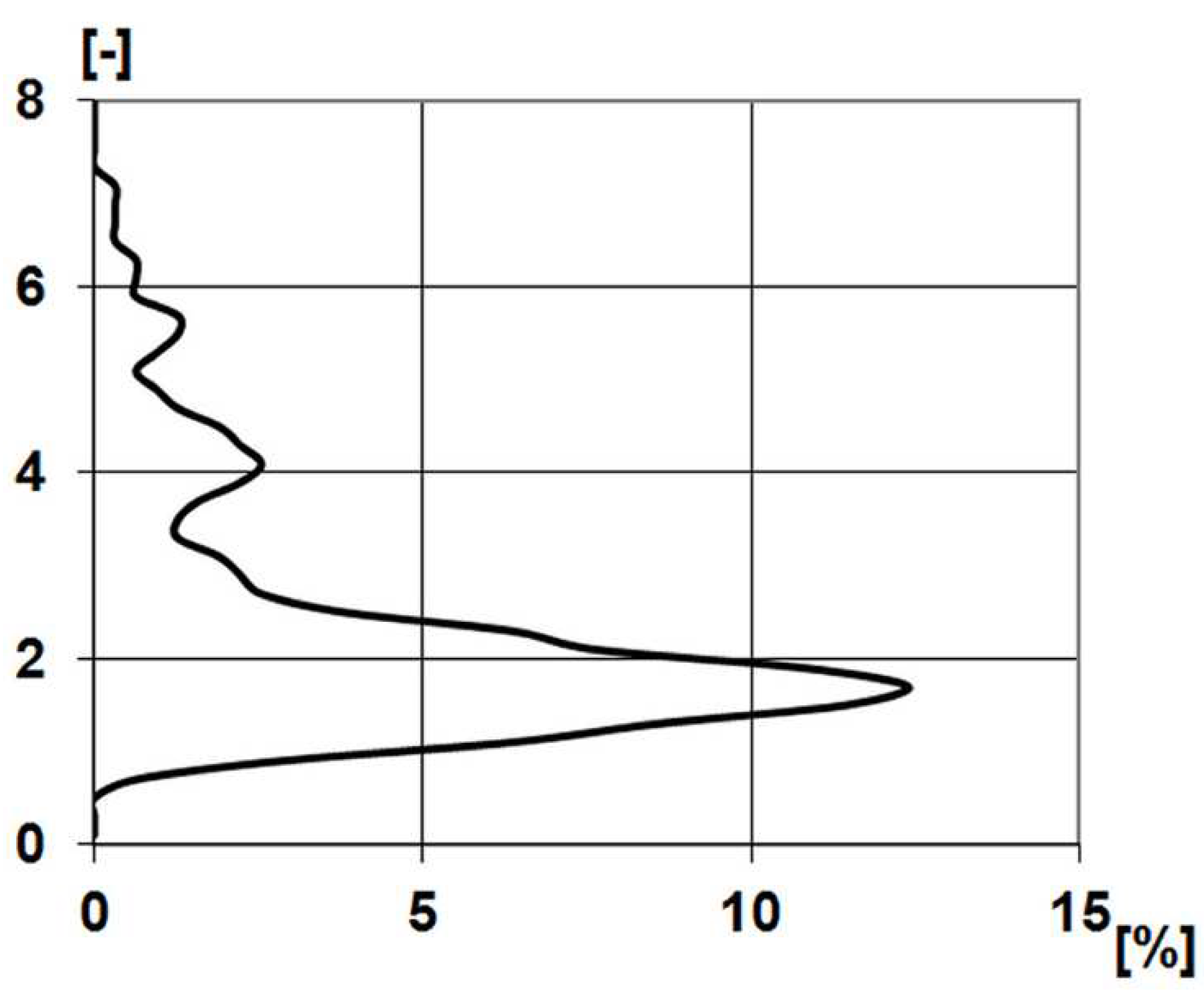
Figure 10.
Measured topography of the plunger; AFM measurement (90 μm by 90 μm measuring area, 352.9 nm by 352.9 nm sampling).
Figure 10.
Measured topography of the plunger; AFM measurement (90 μm by 90 μm measuring area, 352.9 nm by 352.9 nm sampling).
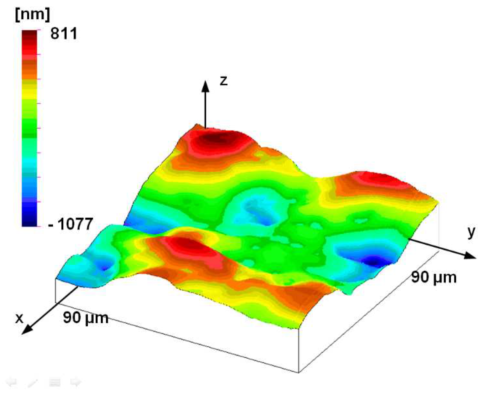
Figure 11.
(a) PSD topography of 3 mm x 3 mm stylus measured surface, (b) PSD curve of 3 mm x 3 mm stylus measured surface.
Figure 11.
(a) PSD topography of 3 mm x 3 mm stylus measured surface, (b) PSD curve of 3 mm x 3 mm stylus measured surface.
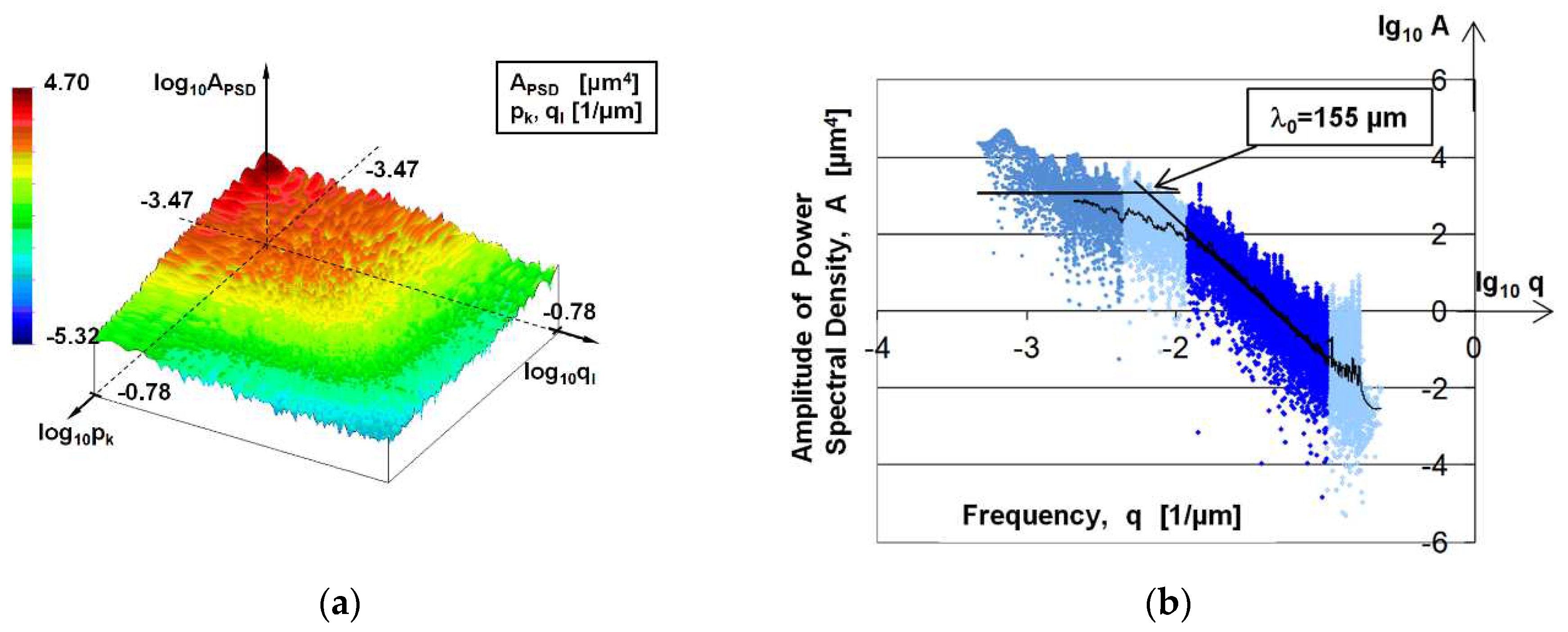
Figure 12.
PSD curve of 25 μm × 25 μm AFM measured surface.
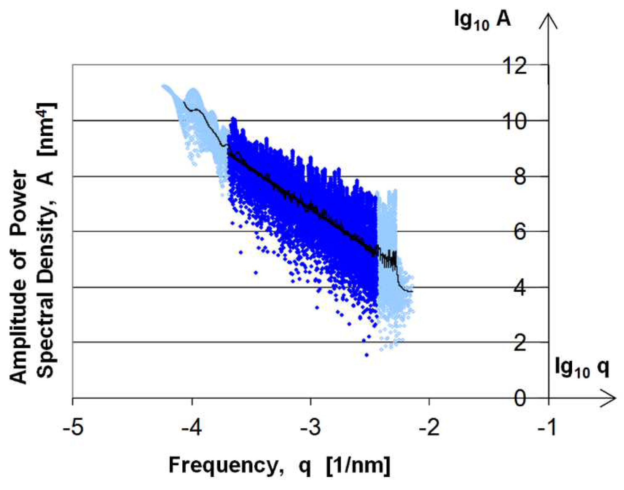
Figure 13.
Fractal dimension sampling distance diagram.
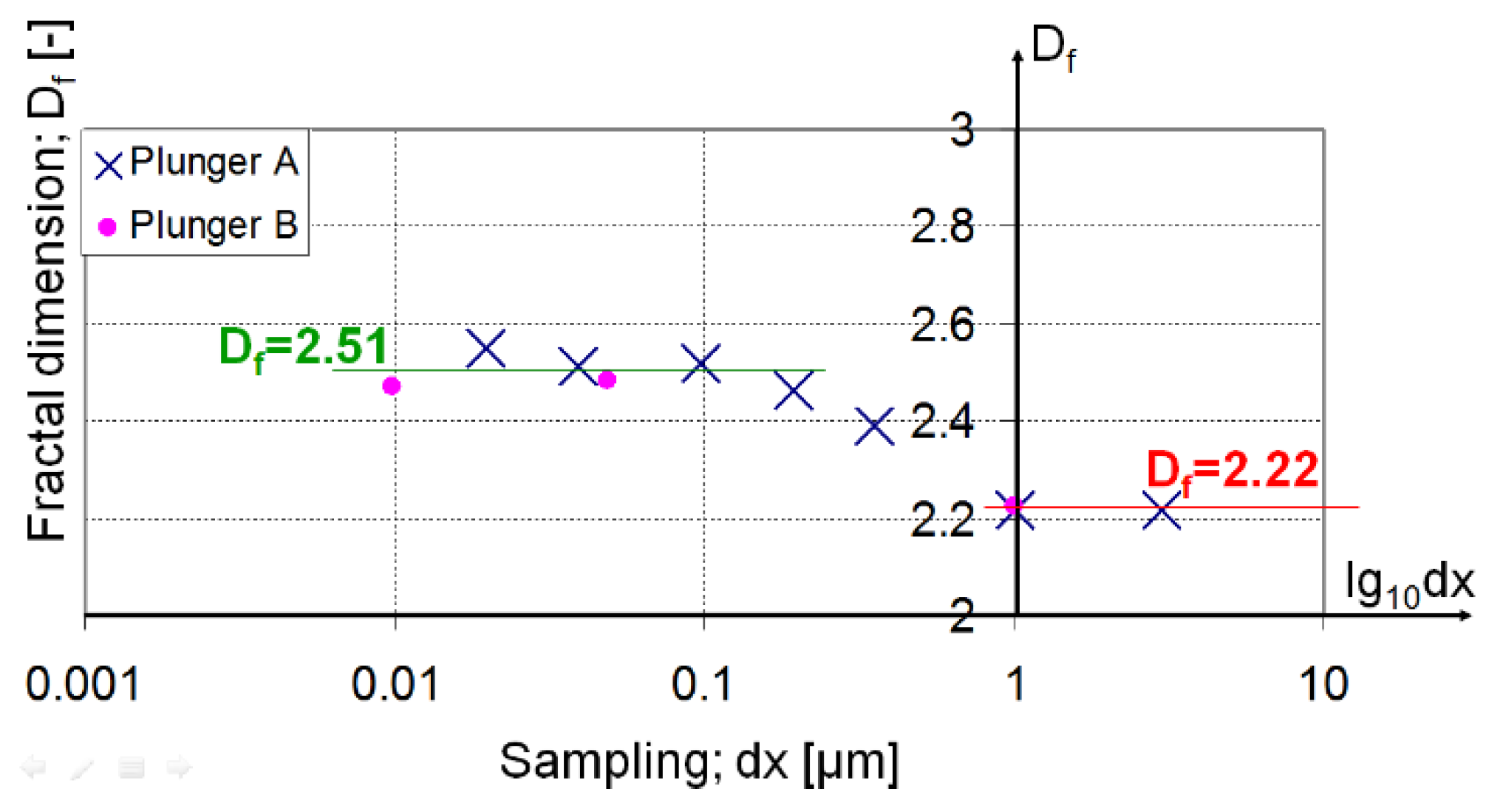
Figure 14.
Measured topography of the plunger; AFM measurement (5 μm by 5 μm measuring area, 19.61 nm by 19.61 nm sampling).
Figure 14.
Measured topography of the plunger; AFM measurement (5 μm by 5 μm measuring area, 19.61 nm by 19.61 nm sampling).
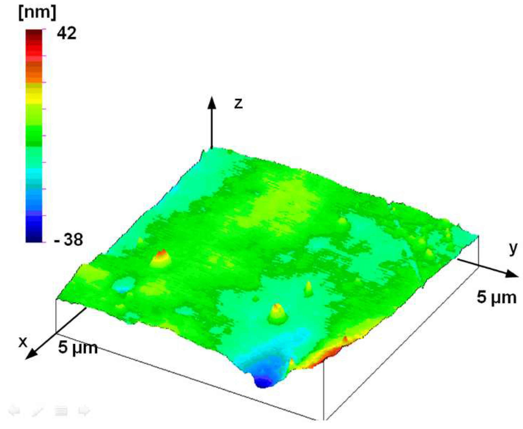

Table 1.
Measuring conditions.
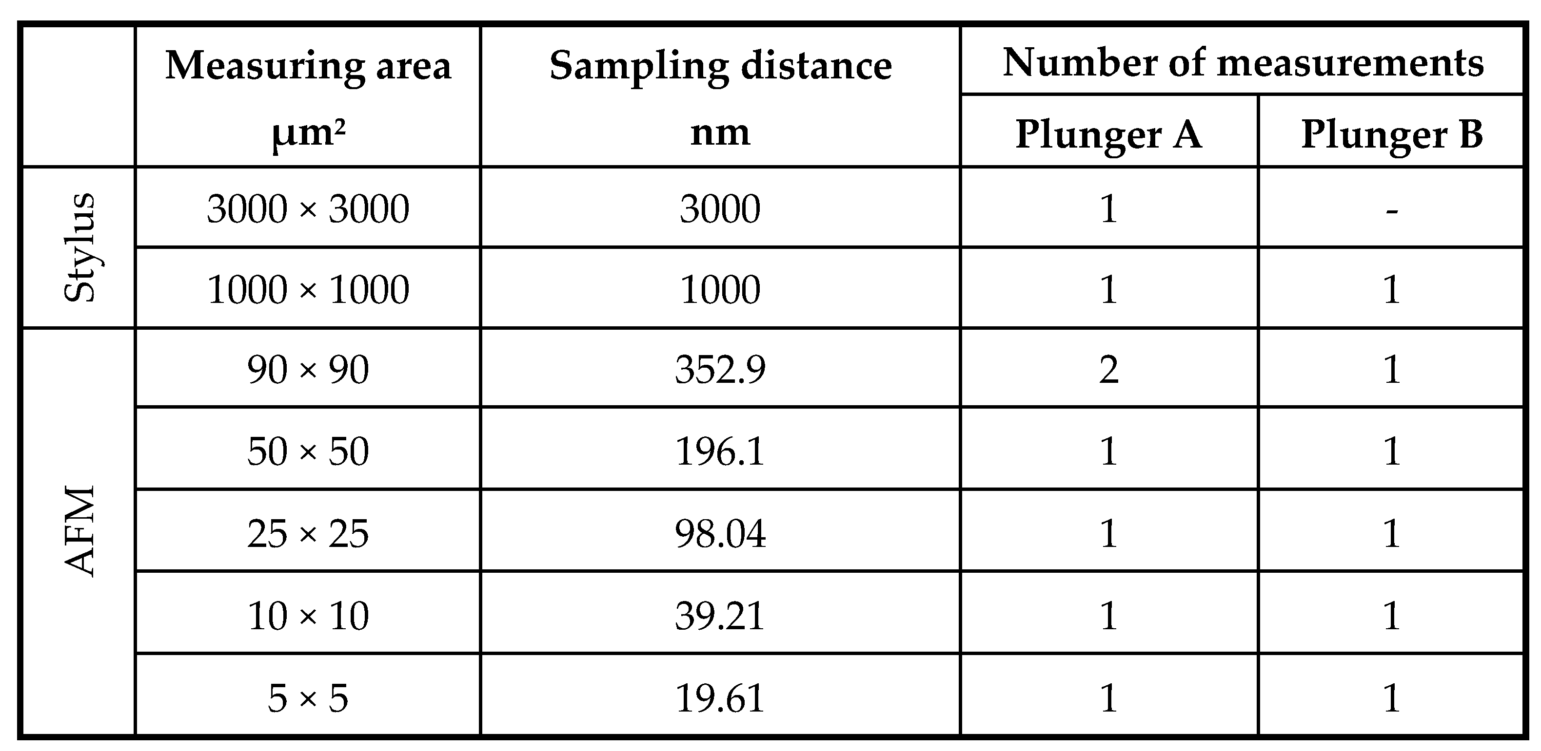 |
Table 2.
Fractal dimensions of topographies.
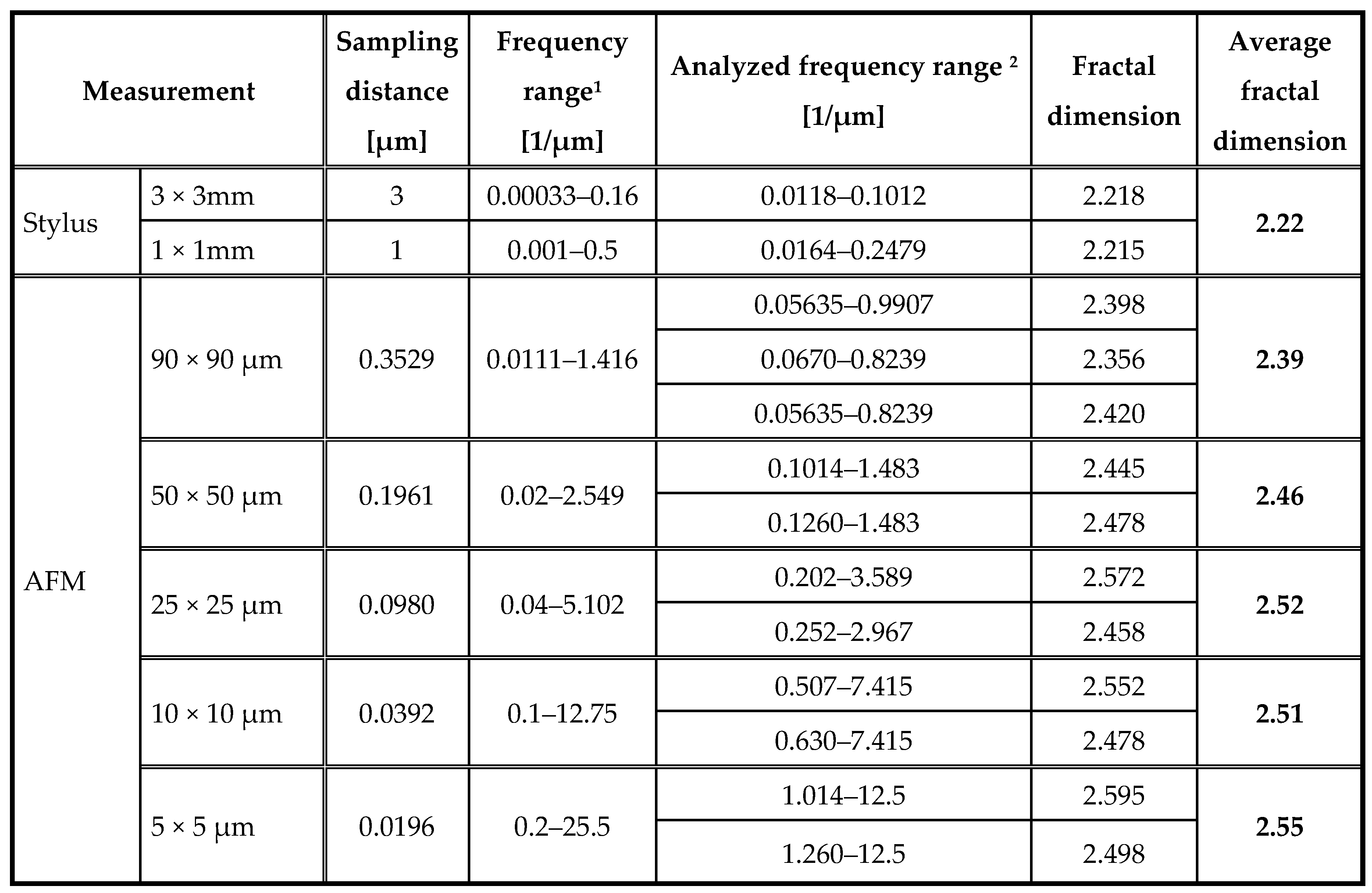 |
1 frequency range depends on the measured area and sampling distance. 2 analyzed frequency range is the range where the line is fitted to PSD curve.
Disclaimer/Publisher’s Note: The statements, opinions and data contained in all publications are solely those of the individual author(s) and contributor(s) and not of MDPI and/or the editor(s). MDPI and/or the editor(s) disclaim responsibility for any injury to people or property resulting from any ideas, methods, instructions or products referred to in the content. |
© 2023 by the authors. Licensee MDPI, Basel, Switzerland. This article is an open access article distributed under the terms and conditions of the Creative Commons Attribution (CC BY) license (http://creativecommons.org/licenses/by/4.0/).
Copyright: This open access article is published under a Creative Commons CC BY 4.0 license, which permit the free download, distribution, and reuse, provided that the author and preprint are cited in any reuse.


